Dynamical evolution of massive black holes in galactic-scale N-body simulations – introducing the regularized tree code “rVINE”

Abstract

We present a hybrid code combining the OpenMP-parallel tree code VINE with an algorithmic chain regularization scheme. The new code, called “rVINE”, aims to significantly improve the accuracy of close encounters of massive bodies with supermassive black holes in galaxy-scale numerical simulations. We demonstrate the capabilities of the code by studying two test problems, the sinking of a single massive black hole to the centre of a gas-free galaxy due to dynamical friction and the hardening of a supermassive black hole binary due to close stellar encounters. We show that results obtained with rVINE compare well with NBODY7 for problems with particle numbers that can be simulated with NBODY7. In particular, in both NBODY7 and rVINE we find a clear N-dependence of the binary hardening rate, a low binary eccentricity and moderate eccentricity evolution, as well as the conversion of the galaxy’s inner density profile from a cusp to a a core via the ejection of stars at high velocity. The much larger number of particles that can be handled by rVINE will open up exciting opportunities to model stellar dynamics close to SMBHs much more accurately in a realistic galactic context. This will help to remedy the inherent limitations of commonly used tree solvers to follow the correct dynamical evolution of black holes in galaxy scale simulations.

1 Introduction

The presence of supermassive black holes (SMBHs; e.g. Rees, 1984) with masses of $10^{6}\hbox{$\mathrm{\thinspace M_{\odot}}$}\lesssim M_{\rm{BH}}\lesssim 10^{10}\hbox{$\mathrm{\thinspace M_{\odot}}$}$ hosted in the central regions of virtually all massive spheroids in the nearby Universe, including the Galactic bulge, is now firmly established (Richstone et al., 1998; Kormendy & Ho, 2013). SMBHs must have also been present at much earlier phases of our Universe, powering active galactic nuclei (AGNs) and quasars from only a few hundred million years after the Big Bang throughout cosmic history (e.g. Lynden-Bell, 1969; Fan et al., 2001; Civano et al., 2011; Mortlock et al., 2011).

We now think of SMBHs as integral components of galactic nuclei, possibly playing a decisive role in shaping the structure and morphology, as well as the gas and thus stellar content of massive galaxies. The $\Lambda\mbox{CDM}$ paradigm for structure formation together with a number of surprisingly tight relations between the SMBH masses and fundamental properties of the galactic bulges hosting them – e.g. the spheroid luminosity (Kormendy & Richstone, 1995) and mass (Magorrian et al., 1998; Häring & Rix, 2004), and the stellar velocity dispersion (Gebhardt et al., 2000; Ferrarese & Merritt, 2000; Tremaine et al., 2002) – suggests co-evolution of the hierarchically growing galaxies and their central black holes (e.g. Lynden-Bell, 1969; Silk & Rees, 1998; Kauffmann & Haehnelt, 2000).

At present, variants of particle-based Smoothed Particle Hydrodynamics (SPH, e.g. Wadsley et al., 2004; Springel, 2005), grid-based Adaptive Mesh Refinement (AMR, e.g. Kravtsov et al., 1997; Teyssier, 2002) codes, or moving mesh codes (Springel, 2010), are the methods of choice for numerical simulations of cosmological galaxy formation, exploiting the high dynamic range and spatial flexibility in resolution. The gravity solvers in these codes either employ a particle-mesh scheme or are tree based and assume the simulated system to be collisionless, with two-body relaxation time-scales exceeding the age of the system. In ’tree’ algorithms (Barnes & Hut, 1986, see also McMillan & Aarseth, 1993 for a collisional tree code) the gravitational force on a single particle from a distant group of particles is approximated by a multipole expansion about the group’s centre of mass, and the N-body particles represent massive tracer particles that sample the underlying smooth gravitational potentials. To reduce the graininess of the potential, gravitational forces are ’softened’ on small spatial scales and the softening length $\varepsilon$ is the natural resolution limit of the code. Unfortunately, this also means that close two-body encounters with a massive body such as a supermassive black hole can - by construction - not be computed accurately. An alternative, much more cost-intensive approach of calculating the gravitational forces in an astrophysical system is the direct summation of each particle’s gravity on every other particle in the system. Combined with high-order integrators, this method is a very accurate way to calculate the gravitational forces and is widely used to simulate collisional N-body systems (e.g. Aarseth, 1999, 2003b; Hut et al., 2010).

Owing to the inherent limitations in the numerical methods, studies of stellar dynamics in the vicinity of SMBHs to date could only probe single separate aspects of the full problem. On the one hand, direct N-body simulations on SMBH binary dynamics in the centres of isolated galaxies or merger remnants (e.g. Ebisuzaki et al., 1991; Milosavljević & Merritt, 2001; Milosavljević & Merritt, 2003; Berczik et al., 2006; Merritt et al., 2007; Khan et al., 2011, 2012; Preto et al., 2011) use idealized initial conditions to represent the inner parts of galaxies in which the massive binaries are then embedded and evolved. Due to the steep scaling of required computing time with particle number of order $\mathcal{O}(N^{2})$ these studies are still rather limited in the particle number, hindering a self-consistent treatment of full galactic environments. On the other hand, simulations of galaxy mergers or cosmological simulations of structure formation including SMBHs (e.g. Springel et al., 2005; Di Matteo et al., 2008; Johansson et al., 2009; Booth & Schaye, 2009; Martizzi et al., 2012; Choi et al., 2012; Sijacki et al., 2014) have difficulties to capture the dynamics of SMBHs and their surrounding stars below the resolution limit. This leads to uncertainties, e.g. in the dynamical friction time-scales for the SMBHs, and affects the density- and velocity-profiles of the stellar background through interactions with the SMBHs, and the hardening and merging time-scales of close SMBH pairs. The latter is generally assumed ’a priori’ to happen fast in these simulations, much reducing the accuracy and predictive power of such simulations. Hence, there is still substantial uncertainty in the current understanding of the dynamical evolution of SMBHs and their surrounding star clusters in realistic cosmological settings, which directly feeds back into uncertainties in our understanding of how SMBH singles or multiples influence the structure of galaxies.

The main goal of this paper is to help remedy these shortcomings by combining the best parts of the two numerical approaches: a regularization method to efficiently and accurately compute the dynamics close to the black holes and a fast tree code to treat the global galactic dynamics. This goes in line with the development of similar recent hybrid codes (as discussed in the next Section) and a software interface designed to efficiently combine different stand-alone code architectures (Portegies Zwart et al., 2009, 2013). With the new algorithm, we will be in a position to better take into account the relevant dynamical processes regarding the interaction between SMBHs and the stars in their environments and other (SM)BHs, in principal without limitations on the spatial and temporal resolution down to scales where other types of physical phenomena become important, e.g. gravitational wave induced coalescence of SMBH binaries or the tidal disruption of low-angular-momentum stars (e.g. Pretorius, 2005; Lodato et al., 2009). This might be an important next step towards investigating the dynamical co-evolution of SMBHs and their host galaxy nuclei in a self-consistent manner in galaxy-scale or cosmological simulations.

In this paper, we present the details of our hybrid N-body code which will help us to focus on the role of gravitational dynamics in the interplay between supermassive black holes and realistic representations of the central regions of their host galaxies. The paper is structured as follows. In Section 2, we describe the details and structure of the new hybrid code “rVINE” and test its performance in Section 4 after we have described the numerical set-up in Section 3. First tests on the code in comparison with the direct N-body code NBODY7 and the tree code VINE are presented in Section 5. We discuss our results in Section 6 and, finally, summarize and draw our conclusions in Section 7.

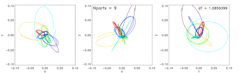
Figure 1: Projected trajectories of regularized particles in the chain around a supermassive black hole. The trajectories are shown in a time interval $\Delta t\approx 1$, which corresponds to $\sim$ one crossing time of the subsystem shown.

2 A new regularized tree code

In this Section we present the structure of the regularized tree code called “rVINE”. A number of currently available N-body codes employ regularization techniques intended for the integration of strong gravitational interactions but are primarily developed for integrations of collisional systems such as star clusters or the dense central regions of galactic nuclei (see Aarseth, 2003a, 2007; Harfst et al., 2008; Gaburov et al., 2009; Nitadori & Aarseth, 2012; Berczik et al., 2013; Wang et al., 2015). In addition, there are two recent hybrid codes combining tree and N-body codes. The BRIDGE code (Fujii et al., 2007) uses a simple fixed time-step oct-tree, while the Bonsai tree code (Bédorf et al., 2012) is an oct-tree run entirely on GPUs. Both hybrids use a symplectic mapping method (Wisdom & Holman, 1991) to couple the tree to a direct N-body algorithm with a fourth-order Hermite integrator.

In rVINE we compute the evolution of a sub-system of particles near the black hole by means of a regularization method, while regions of the galaxy further out with long relaxation times and basically unaffected by the presence of the black hole, are integrated by a collisionless tree code. To this end, we combine two published algorithms: a version of the tree/SPH code VINE (Wetzstein et al., 2009; Nelson et al., 2009) and the algorithmic regularization (AR) chain method (Mikkola & Aarseth, 2002, see also Hellström & Mikkola, 2010 for a general discussion). The latter was kindly provided as a stand-alone code by Seppo Mikkola.

VINE is an OpenMP-parallelized tree/SPH code employing a binary tree algorithm and an individual hierarchical block time-step scheme (Wetzstein et al., 2009; Nelson et al., 2009). The AR-chain method is an efficient and extremely accurate method to study close dynamical few-body encounters and is capable of handling even (repeated) two-body collisions (Mikkola & Aarseth, 2002, see also Preto & Tremaine, 1999; Mikkola & Tanikawa, 1999a, b). This is achieved by effectively removing any singular behaviour in the equations of motion by a time transformation in the Hamiltonian of the regularized sub-system (Mikkola & Aarseth, 2002). The coordinates and the (original) time and their respective ’momenta’ are integrated using a simple leapfrog method. In addition, a Bulirsch-Stoer extrapolation method (Gragg, 1965; Bulirsch & Stoer, 1966) is applied to guarantee high accuracy, as well as a chain concept of smallest inter-particle vectors to reduce round-off errors (Mikkola & Aarseth, 1990, 1993). In our present version of the AR-chain, chain particles are sorted according to their gravitational forces, not according to their distance. It also includes a method to handle velocity-dependent forces, which allows us, in principle, to treat additional viscous and relativistic terms in the regularized force calculations (Mikkola & Merritt, 2006). The new code, however, is purely Newtonian at the present stage.

There exist other regularization schemes which are comparable to the AR-chain in accuracy and speed, e.g. the KS-wheelspoke (Zare, 1974; Aarseth, 2007) and the KS-chain method (Mikkola & Aarseth, 1993). Due to limitations of these methods in the context of stellar dynamics around one or several SMBHs we decided to use the AR-chain as our principal regularization algorithm. For example, large mass ratios may lead to a loss in numerical accuracy for the less massive bodies in a KS-chain, whereas the wheelspoke has difficulties in treating multiple heavy bodies on an equal footing.

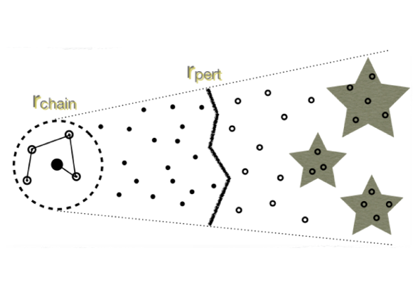
Figure 2: Illustration of the different integration regions near a regularized massive particle in the hybrid AR-regularized tree code. The centre-of-mass reference body, consisting of the members within the regularized subsystem ($r<r_{\rm chain}$), is surrounded by a swarm of nearby particles (’perturbers’) which are considered as external force terms in the chain force calculations ($r<r_{\rm pert}$, where the critical radius $r_{\rm pert}$ depends on a tidal criterion) and, themselves, experience direct N-body forces from the resolved chain (see text). Further out, we indicate the regime where the direct integration of particles (open circles) switches to the multipole approximations, depending on the acceptance criteria in the tree code (indicated by the groups of particles in the large star symbols).

The gravitational forces for the majority of the particles are computed with VINE’s fast binary tree scheme without regularization, using a pre-defined spline or Plummer softening, while particles near a designated massive particle (SMBH) become members of a compact subsystem which is integrated in the AR-chain in its centre-of-mass reference frame.
Chain integration starts if any particle comes closer to the SMBH than $r_{j,\mathrm{BH}}<r_{\rm chain,0}$, where $r_{\rm chain,0}$ defines the initial chain size and is an input parameter which has to be chosen at the start of a simulation as described in the following.

The intended purpose for including particles in the chain integration is twofold. Firstly, we want to accurately follow close orbits near the black holes, i.e. within a fair fraction of the SMBHs’ influence radii, and secondly, we need to overcome the limitations posed by the gravitational softening, i.e. for encounters within $\sim$ a few times $\varepsilon\equiv\max{(\varepsilon_{\rm BH},\varepsilon_{\star})}$, where $\varepsilon_{\star}$ and $\varepsilon_{\rm BH}$ denote the gravitational softening lengths of the stellar particles and SMBHs, respectively. Hence, we determine the initial chain radius,

$$r_{\rm chain,0}=\max(\alpha\cdot r_{\rm infl},\beta\cdot\varepsilon),$$ (1)

at the start of the chain, where $\alpha$ and $\beta$ are input parameters and $r_{\rm infl}$ is the gravitational influence radius of the SMBH. For practical purposes, we define $r_{\rm infl}=\min(r_{\rm infl}^{\rm 2M},r_{\rm infl}^{\rm\sigma})$ using two commonly used proxies for the gravitational influence radius of the SMBH, being 1) the radius enclosing twice the mass of the SMBH, $r_{\rm infl}^{\rm 2M}=r(<2\,M_{\rm BH})$, and 2) the radius within which the gravitational force of the SMBH dominates over the self-gravity of the stellar background, $r_{\rm infl}^{\rm\sigma}=\mathrm{G}M_{\rm BH}/\sigma^{2}$. Here, $M_{\rm BH}$ is the mass of the black hole and G the gravitational constant. The velocity dispersion $\sigma$ is determined by averaging over the nearest $50$ particles outside the chain. We generally find good results for $1\leq\alpha\leq 1.5$ and $1\leq\beta\leq 2$.

The chain’s center-of-mass is treated as a massive particle in the tree, i.e. it is included in the tree force calculations and advanced in time within the tree code. The chain particle is advanced in time on the smallest tree time-step and we formally set the gravitational softening of the chain particle to zero in the tree-code. Tree particles that become members of the chain are converted into ’ghost’ particles with no further advancement in the tree. This is done by assigning a very small, but finite-sized mass in the tree code data structure, rendering their contribution to the gravitational forces negligible. Furthermore, ghost particles are not allowed to determine the size of the time-step in the tree. If the chain is active, the member particles within the chain are advanced using the AR-chain integration, every time particles in the tree code on the smallest time-step level are being advanced.

The equations of motion of the chain members include external forces exerted by a set of nearby tree particles we call “perturbers”, which are identified via a tidal criterion,

$$r_{j,\mathrm{CoM}}<\left(\frac{2}{\gamma_{\rm crit}}\,\frac{m_{j}}{M_{\rm chain}}\right)^{\frac{1}{3}}\times r_{\rm crit},$$ (2)

where $m_{j}$ is the mass of perturber $j$, $M_{\rm chain}$ is the total mass in the chain, and $\gamma_{\rm crit}$ a dimensionless parameter which defines the relative tidal perturbation on the chain. We typically set $r_{\rm crit}=\min(r_{\rm chain},r_{\rm chain,0})$ in the simulations presented here. For better accuracy, the perturber positions relative to the center-of-mass particle are predicted (to 1st order) to the current time at each force calculation in the AR-chain. The perturber forces have to be predicted many times during the numerous sub-step cycles of the Bulirsch-Stoer extrapolations. To improve the overall performance of the chain part of the code we, therefore, have implemented parallel routines for the predictions of the perturbers and the computation of the perturber forces.

Table 1: Parameters for the different N-body calculations.

Simulation,	$N_{\star}$	$M_{\rm tot}$	$r_{0}$	$m_{\star}/M$	$\varepsilon_{\star}$	$N_{\rm BH}$	$r_{\rm BH}^{\rm init}$	$v_{\rm BH}^{\rm init}$	$M_{\rm BH}/M_{\rm tot}$	$\varepsilon_{\rm BH}$
A_Nbody7	100k	1.0	1.0	$10^{-5}$	–	1	2.14	0.46	$10^{-3}$	–
A_Vine-E1/A_Gadget-E1	100k	1.0	1.0	$10^{-5}$	0.02	1	2.14	0.46	$10^{-3}$	0.1
A_Vine-E2/A_Gadget-E2	100k	1.0	1.0	$10^{-5}$	0.02	1	2.14	0.46	$10^{-3}$	0.02
A_rVine	100k	1.0	1.0	$10^{-5}$	0.02	1	2.14	0.46	$10^{-3}$	–
B_Nbody7	10k-100k	1.0	1.0	$10^{-4}-10^{-5}$	–	2	0.1/0	0.28/0	$5\times 10^{-3}$	–
B_Vine	10k-1M	1.0	1.0	$10^{-4}-10^{-6}$	0.01	2	0.1/0	0.28/0	$5\times 10^{-3}$	0.01
B_rVine	10k-1M	1.0	1.0	$10^{-4}-10^{-6}$	0.01	2	0.1/0	0.28/0	$5\times 10^{-3}$	0.01

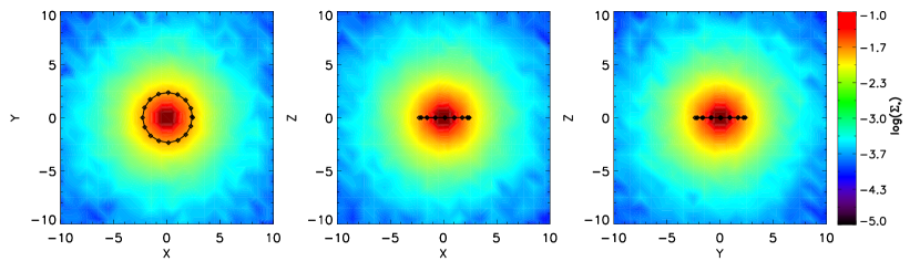
Figure 3: Projections of the initial stellar surface densities (in code units) for a realisation of model A_rVine_100k. The orbital evolution of a SMBH, placed on a circular orbit at the half-mass radius, is shown as the black solid line and symbols for the first orbital period.

Table 2: Parameters for the rVINE calculations.

Simulation	$\alpha$	$\beta$	$\gamma$	$\gamma_{\rm crit}$
A_rVine	1.0	1.0	1.5	$10^{-4}$
B_rVine	$0.1-0.3$	$1.0-4.0$	1.5	$10^{-4}/10^{-5}$

Likewise, the force contributions of individual (’resolved’) chain particles are added to the gravitational forces for the perturber particles during the force updates in the tree. The gravitational force on the chain particle is also corrected by resolving the chain particles. If the chain particle is active, we first calculate the gravitational force exerted on it by particles within the tree code, but subtract the tree forces (i.e. direct, softened N-body interactions) from the perturber particles again. Then the (direct) gravitational force from the perturbers on each individual chain particle is calculated, and added up as a correction to the chain particle’s force according to

$$\vec{a}_{\rm CoM,corr}=\frac{1}{M_{\rm chain}}\sum_{i=1}^{N_{\rm chain}}m_{{\rm chain},i}\,\vec{a}_{{\rm chain},i}.$$ (3)

After advancing the chain one full time-step its membership is updated. Perturber particles are added to the chain if they come closer than the “chain radius”, i.e.

$$r_{j,\mathrm{CoM}}<r_{\rm chain},$$ (4)

where we define the chain radius as the largest distance of any chain member relative to the chain centre-of-mass in the last chain step. Particles are removed from the AR-chain if they recede far enough from the chain’s center-of-mass

$$r_{j,\mathrm{CoM}}>\gamma\times r_{\rm chain,0}\equiv r_{\rm escape}$$ (5)

and move radially away from the chain centre. We typically choose $\gamma=1.5$. Upon removal of a chain member, its mass, position and velocities in the global (i.e. tree) reference frame are restored. If the number of chain members would fall below $N_{\rm chain}<2$ after an escape the chain is terminated and the remaining two chain members are restored in the tree. Likewise, the chain is terminated in the (unlikely) case that the designated massive particle is removed from the chain — unless the chain membership includes several massive particles, in which case one of the remaining SMBHs is chosen to be the new centre-of-mass particle in the tree-code. A representative example of near-Keplerian, perturbed orbits of particles in the chain is illustrated in Figure 1.

The regularization of particle orbits near a designated (massive) particle, leads to different integration regions for different particles in the code, as illustrated in Figure 2. With increasing distance to the chain’s centre-of-mass the particles are either

1. regularized members of the chain (within the dashed circle in Figure 2), feeling external gravitational forces from the perturbers (filled circles) only,

2. perturber particles which feel the gravitational forces of the individual chain members, or

3. tree particles, whose gravitational forces onto the chain particle may either be calculated via direct summation (open circles) or approximated by a multipole expansion of a group of particles (indicated by star symbols), depending on the values for the acceptance criteria chosen in the tree.

For cost reasons, we restrict the total number of chain members and perturbers. We have tested up to values of $N^{\rm max}_{ch}=250$ and $N^{\rm max}_{pert}=5000$ without any loss in the stability of the code.

In short, a typical time-step in the hybrid code proceeds as follows.
(1) Determine the next time-step and active particles for the tree.
(2) If the chain is not active, or, the system does not evolve on the smallest time-step, continue with step (6).
(3) Integrate the members of the chain using the AR-chain method. Treat the external forces exerted by nearby particles (“perturbers”) as perturbations to the members’ gravitational forces.
(4) Check for absorption by and escape from the chain. Perform a search to identify the perturbers via a tidal criterion in regular time intervals (see Equation 2).
(5) Terminate the chain if $N_{\rm chain}<2$.
(6) Perform regular leapfrog time-step in the tree code in the ’drift-kick-drift’ (DKD) scheme:
(a) Update tree particle positions at the half time-step.
(b) Compute gravitational forces for the active tree particles. If the chain particle or any perturber is active include force corrections due to the gravitational forces between the perturber particles and the resolved members of the chain.
(c) Update tree particle positions and velocities at the full time-step.
(7) Update tree particle time-steps in the individual time-step scheme and update the tree structure if necessary.
(8) If the chain is not active check for particles near the SMBH that fulfill the conditions to begin chain regularization.

3 Numerical set-up

In this Section we shortly describe the numerical set-up and the different numerical models we will introduce in the following Sections. In particular, we will detail the way the code works by discussing an example simulation and testing its performance for a number of different code parameters in Section 4. In Section 5 we test the code against a number of other currently available N-body codes, such as the VINE and Gadget-3 tree codes and the NBODY7 direct summation code. All of the rVINE, VINE, or Gadget-3 simulations presented in this paper were run on the COSMOS cluster at DAMTP, Cambridge. For the NBODY7 simulations we used single nodes on the Wilkes cluster at the High Performance Computing (HPC) Service of the University of Cambridge, consisting of a Dell PowerEdge T620 server á 12 Intel Xeon E5-2670 CPUs plus two NVIDIA K20 GPUs.

As our principal numerical model we use a non-rotating Hernquist (1990) sphere to represent the galactic nucleus. The Hernquist density profile follows a $\rho(r)\propto r^{-1}$ power-law at small radii ($r<<r_{0}$) while converging quickly, with $\rho(r)\propto r^{-4}$, to a finite mass at large radii ($r>>r_{0}$). All models are set-up with unit total mass ($M_{\rm tot}=1$) and scale radius ($r_{0}=1$), and the gravitational constant $G$ is set to unity in all codes used throughout this paper. Note that, for convenience, we will use a system of code units in the plots shown throughout the paper. Identifying our model, for instance, with a small spherical (dE/S0) galaxy or a galactic nucleus of mass $M_{\rm tot}=10^{10}\hbox{$\mathrm{\thinspace M_{\odot}}$}$ and scale length $r_{0}=1{\rm\thinspace kpc}$ yields time units and velocity units of $\sim 4.7{\rm\thinspace Myr}$ and $\sim 207{\rm\thinspace km\thinspace s}^{-1}$, respectively. In code units the half-mass radius of the Hernquist sphere is given as $r_{\rm 1/2}=(1+\sqrt{2})\,r_{0}\approx 2.41$ with a half-mass dynamical time of $t_{\rm dyn,h}=27$. In the different simulations considered here the galaxy is realised with total particle numbers in the range $10^{4}-10^{6}$ of equal-mass stellar particles ($m_{\star}\propto N^{-1}$) for VINE and rVINE. For NBODY7, however, we restrict ourselves to $N\leq 10^{5}$ particles due to the steep $\mathcal{O}(N^{2})$ scaling of the direct N-body code. Additionally, we place a few massive particles representing the SMBHs in the simulation, with initial conditions depending on the specific simulation run. Models using a single SMBH are denoted as models ’A’ (Sections 4 and 5.1) while models using two SMBHs are denoted as models ’B’ (Sections 4 and 5.2). To reduce the scatter in our simulations, we will show the results for all models as averages over several independent Monte-Carlo realisations of initial conditions with different random seeds. Depending on $N$, we set up four different realisations for $20$k $\leq N\leq 100$k, two realisations for $100$k $<N<1$M and one realisation for $N=1$M. Details of the set-up together with the explicit name for each simulation run are given in Table 1. As an example, we show the early orbital evolution of a SMBH on the underlying initial stellar surface density for a particular realisation of models ’A_rVine_100k’ in Figure 3 (see also Section 5.1).

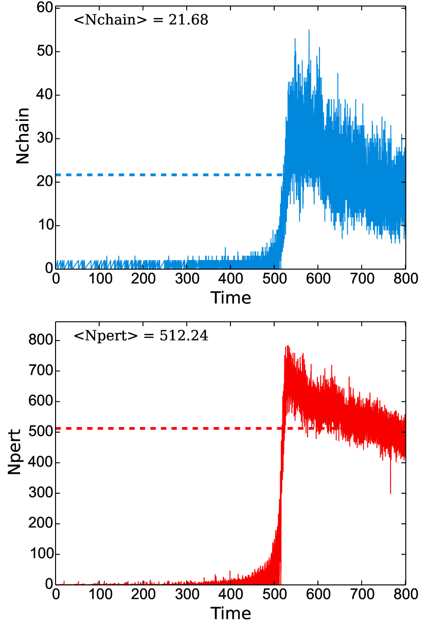
Figure 4: Time evolution of the number of members in the chain and the number of perturbers in a realisation of model A_rVine_100k, with one SMBH initially set on a circular orbit (see Section 5.1). Average numbers are given as text and indicated by the dashed lines.

In all simulations using either VINE or rVINE, we introduce a simple Plummer softening (Aarseth, 1963) with different values for the star particles $\varepsilon_{\star}$ and the SMBHs ($\varepsilon_{\rm BH}$). However, interactions between chain members as well as interactions with the (active) chain centre-of-mass particle in the tree code are not softened at all. For the force calculations in the tree we use a “Gadget” multipole acceptance criterion (MAC) with error tolerance $\theta=10^{-3}$ and conservative values for the accuracy parameters $\tau_{\rm acc,\star}=\tau_{\rm vel,\star}=0.3$ and $\tau_{\rm acc,BH}=\tau_{\rm vel,BH}=0.003$ for the leapfrog integration (see Wetzstein et al., 2009). In the Gadget-3 simulations the same integration accuracy, $\tau=0.02$, is adopted for both stellar and BH particles, along with an error tolerance of $5\times 10^{-3}$. For NBODY7 we set the chain radius to $1.25\times 10^{-3}$ and do not make use of softened gravitational interactions. The total accumulated relative energy error stayed below $\lesssim 10^{-4}$ for all simulations with an accuracy parameter of $\tau_{0}=0.02$. The parameter ranges used to define the perturber particles and chain members (see Section 2) in the rVINE simulations can be found in Table 2 .

4 Testing the code and code performance

In this section, we carry out some basic examples and tests on the code performance of the AR-regularized tree code.

In Figure 4 we illustrate the time evolution of the number of particles in the chain (upper panel) and the number of perturbers (lower panel) for one realisation of model A_rVine_100k, following the orbital evolution of a SMBH in a Hernquist sphere consisting of $N=10^{5}$ particles (see also Section 5.1). The SMBH is assigned a mass of $M_{\rm BH}=10^{-3}\,M_{\rm tot}$ and set on an initially circular orbit at the half-mass radius ($r_{\rm BH}(t=0)=2.41$). As the SMBH sinks to the centre the number of chain members as well as perturbers increases significantly at time $t\sim 520$, i.e. at about the time the SMBH sinks to the central high-density regions within $\lesssim 10$% of the half-mass radius. Shortly after we reach the maximum number of 55 particles in the chain and a maximum number of $\sim 780$ perturbers, while the average numbers are only $\langle N_{\rm chain}\rangle\sim 20$ and $\langle N_{\rm pert}\rangle\sim 500$, respectively. This highlights the need to perform some exploratory simulations to determine whether rVINE can actually handle the range of particle densities around the SMBH encountered over the simulated time span.

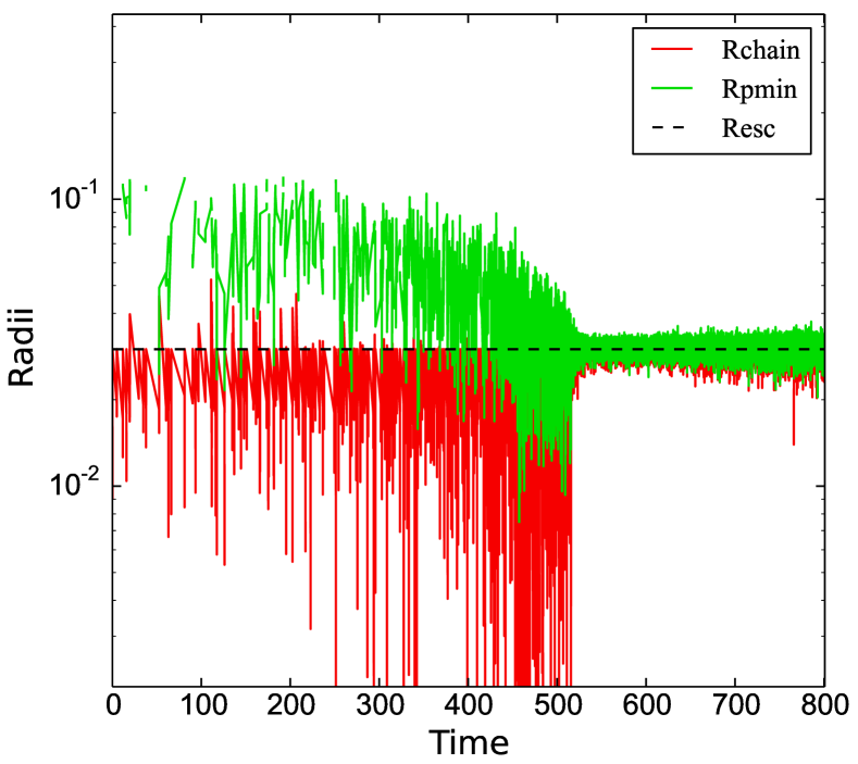
Figure 5: Time evolution of characteristic radii in a realisation of model A_rVine_100k, with one SMBH set on a circular orbit (see Section 5.1): the radius of the chain (red solid line), the distance of the nearest perturber to the chain centre-of-mass (green solid line) and the radius of escaping chain particles (black dashed line).

Overall, a fraction of $6.9\%$ of the $10^{5}$ particles, was subject to integration in the chain during this run. Chain integration was active for a total of $42\%$ of the total run time, $t_{\rm max}=800$. At the early stages of the simulation, the chain is used only intermittently to treat the occasional strong stellar encounters near the SMBH in the low density environment. At later phases, when the SMBH is near to the centre, the chain is used more intensively, with the chain being active continuously for $\sim 285$ time units. Stellar particles are typically included repeatedly in the chain with an average number of $\sim 8$ recurrences.

Figure 5 shows the corresponding time evolution of some characteristic radii from the simulation shown in Figure 4. The escape radius (black dashed line), given by Equation (5), serves as an effective upper bound for the chain radius (red solid line). For times $t\lesssim 300$ the minimum disturber distance, $r_{\rm p,min}$, (green solid line) is generally well above the escape radius, before some perturbers may come closer to a chain that has only a few and, by chance, quite compact members while the SMBH is sinking to denser central regions ($300\lesssim t\lesssim 520$). Once the SMBH is close to the centre of the Hernquist sphere ($t\gtrsim 550$) and the number of particles in the chain has increased by a factor of ten, $r_{\rm chain}$ and $r_{\rm p,min}$ both oscillate around $r_{\rm escape}$, which naturally arises when a number of particles lives close to the conditions for both absorption and escape being satisfied at a certain time. In this case, in rVINE we prioritise the absorption of near perturbers over a (delayed) escape of a chain member, until the chain radius has grown by $5\%$ over the nominal escape radius. A noticeable oscillation around the escape radius can then occur if a series of subsequent absorptions of perturbers near the SMBH takes place.

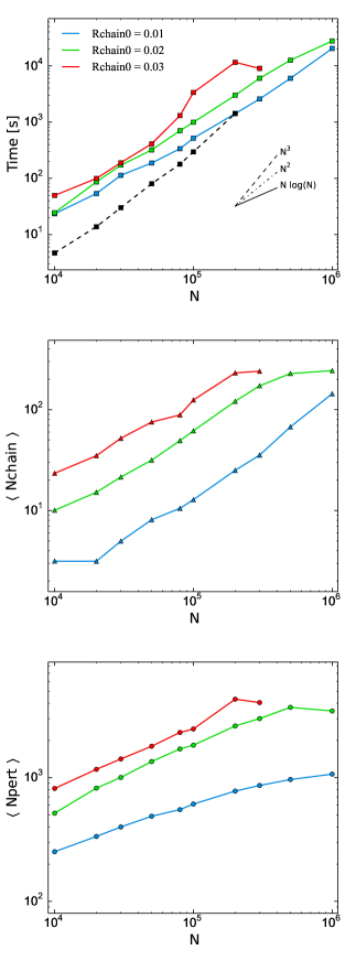
Figure 6: Performance characteristics for the rVINE code as a function of varying initial chain radii in calculations of two SMBHs at the centre of a Hernquist sphere, one being set on a circular orbit at $x_{\rm BH1}=0.1$ and the other one being at rest at the origin (see also Section 5.2). The three panels show the code run time in seconds (top), the average number of particles in the chain (middle), and the average number of perturbers (bottom) versus the total number of stellar particles in the simulations. All runs were evolved for one code time unit ($\Delta{t}=1$).

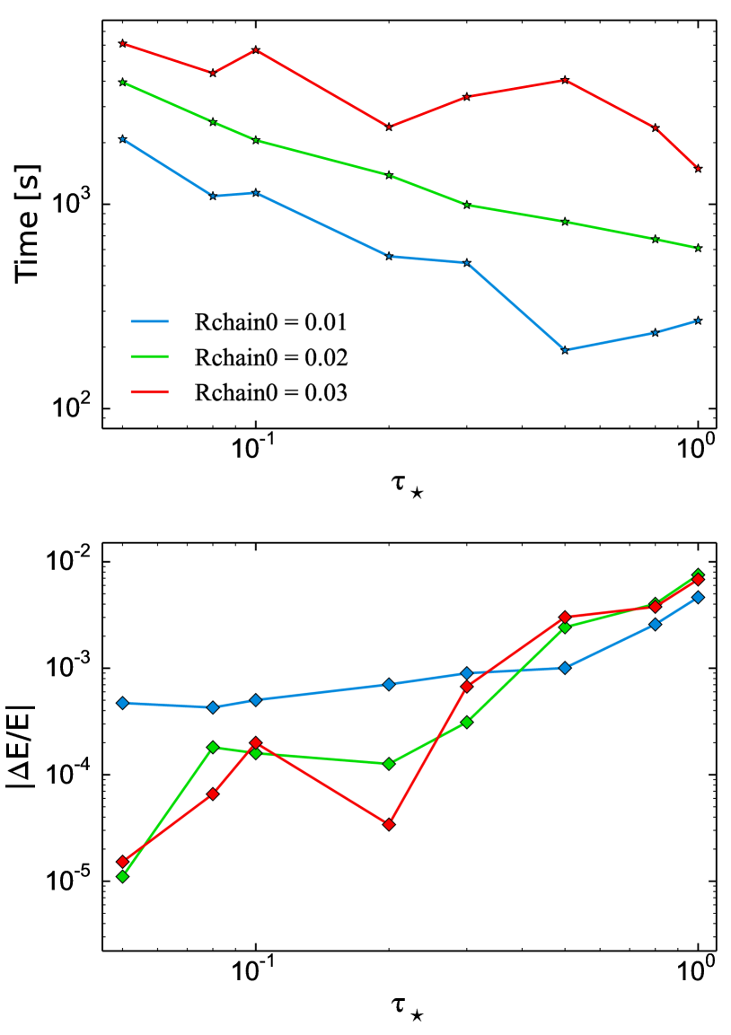
Figure 7: Performance characteristics for the rVINE code as a function of varying initial chain radii for the model used in Figure 6. Shown are the code run time (top panel) and the relative energy error (bottom panel) versus the accuracy parameter of the tree code time-step criteria, $\tau_{\star}$. All runs were evolved for one code time unit ($\Delta{t}=1$).

In Figures 6 and 7 we investigate the performance characteristics of rVINE using a set of simulations of our basic Hernquist model with two SMBHs, each having a mass of $M_{\rm BH}=5\times 10^{-3}\,M_{\rm tot}$. One of the SMBHs is initially set on a circular orbit close to the centre ($x_{\rm BH1}=\pm 0.1$ and $v_{\rm y,BH1}\approx 0.28$), the other one is at rest at the origin (models B_Vine and B_rVine; see also Section 5.2). All runs shown in Figures 6 and 7 were performed on a single node (8 CPUs) of Cosmos2, except for a few comparison runs using NBODY7 (see Figure 6, upper panel) which were performed using 8 CPUs plus acceleration from two NVIDIA K20 GPUs on the Wilkes cluster.

The three panels in Figure 6 show the wall clock time required to evolve the simulation to $t=1$ (upper panel), as well as the average number of particles in the chain (middle panel) and the average number of perturber particles (bottom panel) as a function of the initial chain radius $r_{\rm chain,0}$ and particle number $N$. Interestingly, the run time does not seem to depend strongly on the choice of the initial chain radius; it typically changes by a factor of $\sim$ a few, and at most by a factor of $\sim 8$, when varying $r_{\rm chain,0}$ up to a factor of 3. In addition, the scaling with $N$ is still relatively shallow for all initial chain radii as the computing time is dominated by the tree. For comparison, we show the scaling obtained with NBODY7 using the same initial conditions for $N\leq 2\times 10^{5}$ (black dashed line). Due to the fact that we can use the additional acceleration of the two NVIDIA K20 GPUs (plus some contribution from running on a different system) the total computing time is actually a factor of $\sim 5$ to $\sim 10$ times lower compared to rVINE at the lowest particle numbers. However, the steeper scaling of NBODY7 ($T_{\rm wall}\propto N^{1.9}$) yields comparable computing times already for $N\gtrsim 2\times 10^{5}$. Extrapolating this scaling would give clear advantages to rVINE for $N\gtrsim 10^{6}$ particles in that particular case.

The average number of particles in the chain shows a roughly linear scaling with total particle number for $N>2\times 10^{4}$ while the average number of perturbers has a shallower N-dependence. The latter can be understood by considering the fact that the region of the perturber particles actually becomes smaller with increasing $N$, since the mass of the perturbers scales as $\propto N^{-1}$ (see Equation (2)). Hence, if the number of particles in the chain were to scale strictly linearly with $N$, or in the limit of the SMBH dominating the total mass of the chain, e.g. for a high SMBH-to-star mass ratio and small $r_{\rm chain,0}$, we would expect $\langle N_{\rm pert}\rangle$ to be largely independent of $N$. The observed shallow increase of $\langle N_{\rm pert}\rangle$ with $N$ is likely to be caused by the non-trivial non-linear scaling $\langle N_{\rm chain}\rangle$ observed in the middle panel. Both $\langle N_{\rm chain}\rangle$ and $\langle N_{\rm pert}\rangle$ show a scaling going roughly as $N\propto r_{\rm chain,0}^{2}$, as expected for the central parts of the Hernquist profile, where $M(r)\propto r^{2}$ (see Hernquist, 1990, their equation (3)).

The upper panel of Figure 7 shows the total run time of the simulations as a function of the accuracy parameter for the tree code time-step criteria, $\tau_{\star}$. In principle one is free to choose different values for the different time-step criteria used in VINE (see Section 3 and equations (10) - (12) in Wetzstein et al., 2009), but we decided to adopt one, identical value of $\tau_{\star}$ for all criteria and fixed the particle number at $N=10^{5}$. The time-step size increases linearly with $\tau_{\star}$ leading to an overall decrease in the run time for all values of $r_{\rm chain,0}$, albeit with some non-negligible scatter. Within the scatter, the total wall time scales roughly as $T_{\rm wall}\propto r_{\rm chain,0}$ for fixed $\tau_{\star}$. In the lower panel of Figure 7, we show the energy conservation of the code for a given time-step accuracy. To avoid spurious energy errors upon start-up, we have measured the energy errors in the interval from $t=4$ to $t=5$. The calculations become generally less accurate for larger time-step sizes as expected. However, especially for values of $\tau_{\star}\leq 0.3$, the scaling is much steeper for larger values of $r_{\rm chain,0}$. i.e. when a larger fraction of tree code particles are integrated in the more accurate chain. For the simulations with $r_{\rm chain,0}=0.02$ and $r_{\rm chain,0}=0.03$ the relative energy error scales roughly as $\propto\tau_{\star}^{2}$.

5 Comparison with analytical estimates and other codes

5.1 Dynamical friction of a SMBH in a Hernquist sphere

As a first test of rVINE, we investigate the orbital evolution of a massive particle due to dynamical friction in a spherical non-rotating Hernquist sphere (model A), comparing results from different simulations using NBODY7, rVINE, VINE, and Gadget-3. The massive particle of mass $M_{\rm BH}=10^{-3}\,M_{\rm tot}$ is set on an initially circular, co-rotating orbit at the half-mass radius ($r_{\rm BH}(t=0)=2.41$) (see also Section 3).

\begin{picture}(14.5,22.0)\put(0.0,16.2){\epsfbox{./fig8a}} \put(0.0,10.8){\epsfbox{./fig8b}} \put(0.0,5.4){\epsfbox{./fig8c}} \put(0.0,0.0){\epsfbox{./fig8d}} \end{picture}

Figure 8: Comparison of the distance to the centre (left panels) and velocity (right panels) of a single SMBH, initially set on a circular orbit at the half-mass radius of a Hernquist sphere, for different code architectures. From top to bottom we show the direct summation code NBODY7 (blue; model A_Nbody7_100k), the AR-chain regularized tree code rVINE (red; model A_rVine_100k), and the VINE and Gadget-3 tree codes (green and pale blue lines) with varying softening lengths, $\varepsilon_{\rm BH}=0.1$ (models A_Vine-E1_100k and A_Gadget-E1_100k) and $\varepsilon_{\rm BH}=0.02=\varepsilon_{\star}$ (models A_Vine-E2_100k and A_Gadget-E2_100k). Theoretical expectations from dynamical friction theory are given as black lines for different parameters of $\kappa_{\rm s}$ ($\kappa_{\rm s}$ parametrizes the deviation from a locally isotropic Maxwellian velocity distribution, see Section 5.1). For comparison, we show the results for the NBODY7 run also in the other panels. rVINE very well recovers the expected orbital evolution by effectively removing the limitations imposed by gravitational softening. Results shown are averages over several realisations of the initial conditions, as described in the text.

5.1.1 Dynamical friction theory

For a meaningful assessment of the different codes, we compare the simulated SMBH trajectories with theoretical expectations from dynamical friction theory (Chandrasekhar, 1943; Binney & Tremaine, 2008). Assuming a locally isotropic velocity distribution function, a homogeneous density $\rho$, as well as a sufficiently large velocity of the SMBH, $v_{\rm BH}$, relative to the stellar background, the rate of deceleration of the SMBH due to dynamical friction may be given by the standard formula (cf. Binney & Tremaine, 2008, Eq. 8.5)

$$\vec{a}_{\rm DF}=-4\pi\,{\rm G}^{2}\frac{M_{\rm BH}}{v^{3}_{\rm BH}}\,\rho(v<v_{\rm BH})\,\ln\Lambda\ \vec{v}_{\rm BH},$$ (6)

where $\ln\Lambda$ is the Coulomb logarithm. Only the mass density of stars moving slower than the SMBH, $\rho(v<v_{\rm BH})$, contributes to the dynamical friction. With gravitational softening there is a limit on the maximum gravitational force that may be exerted in any star-SMBH encounter through an effective minimum impact parameter ${\rm b}_{\rm min}$ (see e.g. White, 1976; Just et al., 2011),

$${\rm b}_{\rm min}=1.5\cdot\max(\varepsilon_{\star},\varepsilon_{\rm BH}).$$ (7)

Taking this softening effect into account, we write the Coulomb logarithm as

$$\ln\Lambda=\ln\left(\frac{{\rm b}_{\rm max}}{\sqrt{{\rm b}_{\rm min}^{2}+{\rm b}_{\rm 90}^{2}}}\right),$$ (8)

where ${\rm b}_{\rm max}$ is the maximum impact parameter and ${\rm b}_{90}$ is the impact parameter for a $90^{\circ}$ scattering event of the incident star. The choice for the latter two parameters is often rather arbitrary, with ${\rm b}_{90}$ depending on the typical velocity $v_{\rm typ}$ of the stars. The maximum impact parameter ${\rm b}_{\rm max}$ is often taken proportional to the orbital radius of the SMBH $r_{\rm BH}$. Following Just & Peñarrubia (2005), we identify ${\rm b}_{\rm max}$ with the local scale length,

$${\rm b}_{\rm max}=\frac{\rho}{|\nabla\rho|}=\frac{r_{\rm BH}}{3-\eta},\ \ \eta\leq 2,$$ (9)

where the last equation is true for the family of $\eta$-models (Dehnen, 1993; Tremaine et al., 1994) if $\eta\leq 2$. Hence, in the case of the Hernquist profile ($\eta=2$) we obtain that the maximum impact parameter exactly equals the orbital radius of the SMBH, i.e. ${\rm b}_{\rm max}=r_{\rm BH}$. In addition the $90^{\circ}$ deflection parameter is given by

$${\rm b}_{90}=\frac{{\rm G}\,M_{\rm BH}}{v_{\rm typ}^{2}}\approx\frac{{\rm G}\,M_{\rm BH}}{2\sigma^{2}+v_{\rm BH}^{2}}.$$ (10)

Using Equations (6) - (10), we evolve the orbit of a SMBH, initially placed on a circular orbit at the half-mass radius, in the analytic Hernquist potential including the additional drag forces due to dynamical friction with a leapfrog integrator. The density of stars with velocities smaller than the SMBH is represented as

$$\rho(v<v_{\rm BH})=\kappa_{\rm s}\cdot\rho_{\rm s}(v<v_{\rm BH}),$$ (11)

where $\rho_{\rm s}(v<v_{\rm BH})$ denotes a locally isotropic Maxwellian velocity distribution given by

$$\rho_{\rm s}(v<v_{\rm BH})=\rho(r)\times\left[\mathrm{erf}(X)-\frac{2X}{\sqrt{\pi}}\mathrm{e}^{-X^{2}}\right]$$ (12)

where $X\equiv v_{\rm BH}/\sqrt{2}\sigma$ with dispersion $\sigma$, and erf$(X)$ is the error function (Binney & Tremaine, 2008). We use $\kappa_{\rm s}$ as a free parameter to account for the fact that the velocity distribution of the Hernquist model does not follow a simple Maxwellian distribution, as often used as an approximation in dynamical friction calculations. Hence, the locally isotropic Maxwellian velocity distribution corresponds to $\kappa_{\rm s}=1.0$.

5.1.2 Results

The upper panels of Figure 8 show the evolution of the radial decay (left) and the velocity (right) of the SMBH with time for model A_Nbody7_100k. NBODY7 is very well suited to follow the dynamical friction of the heavy body. We gauge run A_Nbody7_100k (blue line) against theoretical orbits for different values of $\kappa_{\rm s}=(0.5,0.75,1.0)$ shown as black lines and use it subsequently as a reference for the other simulation codes. Initially the orbital evolution follows quite closely the analytic prediction with $\kappa_{\rm s}=0.75$ (black dotted line). At smaller central distances ($r\lesssim 0.6\,r_{\rm BH}^{\rm init}$) the dynamical friction seem to act even more efficiently in the full N-body run. This leads to a slightly faster orbital evolution such that the SMBH reaches the centre (defined as $r\lesssim r(M<2\,M_{\rm BH})$, where dynamical friction ceases to be efficient) within $t\lesssim 500$ time units. In the second row of Figure 8 we compare the efficiency of dynamical friction on the SMBH in model A_rVine_100k (red line) and model A_Nbody7_100k (blue line). We find that the early orbital evolution ($r>0.5\,r_{\rm BH}^{\rm init})$ in model A_rVINE_100k is nearly indistinguishable from the one in model A_Nbody7_100k such that the SMBH reaches the centre on a very similar timescale, only about $\sim 8\%$ longer than in model A_Nbody7_100k, in very good agreement with the NBODY7 result.

On the other hand, owing to their inherent resolution limitations, we expect the tree codes to show a significantly slower radial decay depending on the adopted gravitational softening, via Equation (7). If the SMBH is treated as a quasi collisionless particle with a large gravitational softening length ($\varepsilon_{\rm BH}=0.1$, third row), it decays to only about half its original distance within the time span ($t\sim 960$) shown in the Figure 8 in both model A_Vine-E1_100k (green line) and model A_Gadget-E1_100k (pale blue line). The total time to reach the centre is $t\gtrsim 1350$ time units for both codes, significantly longer (by a factor of $\gtrsim 2.7$) than with NBODY7. This can be understood as a result of the reduced frictional force for near encounters. Both codes, however, follow the analytical prediction with $\kappa_{\rm s}=0.75$ if we adopt the minimal impact parameter ${\rm b}_{\rm min}=1.5\cdot\varepsilon_{\rm BH}$ from Equation (7). Setting $\varepsilon_{\rm BH}\equiv\varepsilon_{\star}=0.02$ (bottom row) yields an enhancement in the near encounters, but the decay time to the centre is still about $50\%$ ($70\%$) longer than in the NBODY7 case for model A_Vine-E1_100k (A_Gadget-E1_100k). Hence, even this drastic reduction in the gravitational softening of the SMBH does not significantly improve the accuracy of the dynamical friction time-scale.

While all codes capture the effects of dynamical friction as expected, if we consider softened gravitational force terms, this highlights the importance of an accurate treatment of close encounters for the correct description of dynamical friction in N-body tree codes. From our analysis we conclude that the AR-regularized tree code removes the limitations due to the gravitational softening of the SMBH imposed on present-day tree codes by including nearby particles in the chain.

5.2 Evolution of a SMBH binary at the centre of a Hernquist sphere

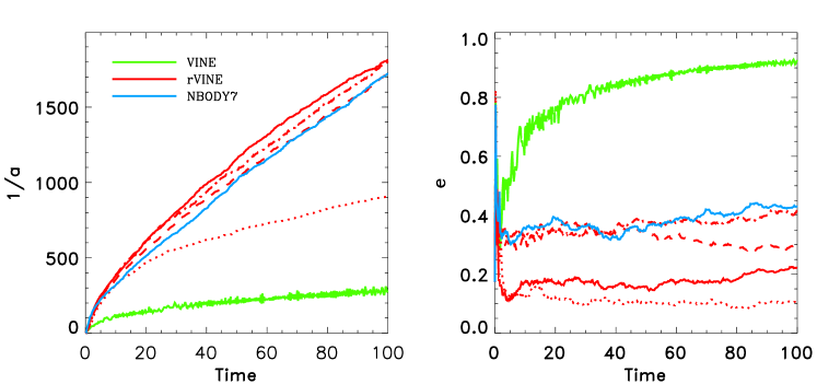
Figure 9: Evolution of binary parameters of a SMBH binary at the centre of a non-rotating Hernquist sphere (model B). Shown are binary hardness ($1/a$, left panel) and eccentricity (right panel) as a function time. Different colours indicate simulations using different codes, i.e. NBODY7 (blue), VINE (green, with $\varepsilon_{\rm BH}=\varepsilon_{\star}$), and rVINE (red lines). Different line styles for model B_rVine denote different runs with varying initial chain radii ($r_{\rm chain,0}=0.01$: dotted, $0.02$: solid, $0.03$: dashed, and, $0.04$: dot-dashed). The results shown are averages over several realisations of the initial conditions, as described in the text.

Another crucial test for rVINE is to investigate the hardening of a SMBH binary, compared to results obtained with NBODY7 and VINE. For our model B, we choose an initial set-up similar to the one presented in Merritt et al. (2007) and Vasiliev et al. (2014). In particular, we set up two SMBHs at the centre of a non-rotating Hernquist sphere with masses $M_{\rm BH}=5\times 10^{-3}\,M_{\rm tot}$ and one of the SMBHs on a circular orbit ($x_{\rm BH1}=0.1$, $v_{\rm y,BH1}=|v_{\rm circ}|\approx 0.28$) and the other SMBH at rest at the origin. For models B_Vine and B_rVine we use gravitational softening lengths $\varepsilon_{\star}=0.01=\varepsilon_{\rm BH}$ for the stellar and SMBH particles in the tree-code. Particles in the chain are not softened. The initial distance is chosen slightly larger than the influence radii of the SMBHs, which typically increase in the B_rVine and B_Nbody7 runs from $r_{\rm infl}^{\rm 2M}\approx 0.1$ to $r_{\rm infl}^{\rm 2M}\approx 0.16$ according to a decrease in the central density during the simulations. In the simulations using model B_rVine, initially, only the co-rotating SMBH is regularized, but quickly – for $t\lesssim 1.5$ — the second SMBH is captured into the chain. In the B_Nbody7 runs we use an AR-chain with a chain radius of $R_{\rm chain}=1.25\times 10^{-3}$, while we test different values of the initial chain radius for the AR-chain in rVINE which we set to a size comparable to the hard binary semi-major axis, $r_{\rm chain0}\sim\mathrm{a\ few}\times a_{\rm hard}$. The hard binary semi-major axis is given as

$$a_{\rm hard}=\frac{\mu}{M_{\rm BH1}+M_{\rm BH2}}\frac{r_{\rm infl}^{\rm 2M}}{4},$$ (13)

with $\mu=(1/M_{\rm BH1}+1/M_{\rm BH2})^{-1}$ being the reduced mass. Initially, $a_{\rm hard}=r_{\rm infl}^{\rm 2M}/16\approx 6.25\times 10^{-3}$.

In Figure 9 we show the time evolution of the SMBH binary hardness ($1/a$, left panels) and eccentricity (right panels) for the first $t=100$ time units in the simulations of model B with $N=10^{5}$ particles. If we set a large initial chain radius, $r_{\rm chain,0}=0.02$ (red solid lines), $r_{\rm chain,0}=0.03$ (red dashed lines), or $r_{\rm chain,0}=0.04$ (red dot-dashed lines), model B_rVine_100k agrees well with model B_Nbody7_100k (blue lines) showing an efficient hardening with a nearly constant hardening rate $\frac{d}{dt}(1/a)$ for $t\gtrsim 10$, and a rather mild binary eccentricity ($e<0.4$). On the other hand, when setting the initial chain radius comparable to $a_{\rm hard}$ and the softening parameter, $r_{\rm chain,0}=0.01$ (red dotted lines), the hardening of the SMBH binary proceeds much slower since we start to miss out on some close encounters with the hard binary, owing both to the effect of softening and the lower cross-section of the chain. Model B_Vine_100k (green lines), on the other hand, shows a qualitatively different picture, with a significantly larger separation between the two SMBHs ($1/a\approx 300)$ and a high binary eccentricity of $e\lesssim 0.95$ at the end of the simulations. While the reduced binary hardening is clearly due to both the softened gravitational forces near the SMBHs and the reduced rate of loss-cone refilling in the collisionless tree-code, the reason for the high binary eccentricity is unclear.

\begin{picture}(15.3,21.6)\put(0.0,14.4){\epsfbox{./fig10a}} \put(0.0,7.2){\epsfbox{./fig10b}} \put(0.0,0.0){\epsfbox{./fig10c}} \end{picture}

Figure 10: Time evolution of binary hardness ($1/a$, left panels) and eccentricity (right panels) as a function of particle number N for the three different codes in model B: NBODY7 (top row), rVINE (middle row) and VINE (bottom row). Shown are simulations with particle numbers increasing from $N=20$k to $N=1M$ from top to bottom, with colours indicated in the legend. The initial chain radius is set to $r_{\rm chain,0}=0.02$ in the simulations of model B_rVine. The results shown are averages over several realisations of the initial conditions, as described in the text.

Figure 10 extends the analysis of Figure 9 to a range of different particle numbers. For VINE and rVINE we investigate simulations with particle numbers ranging from $N=2\times 10^{4}-10^{6}$ and between $N=2\times 10^{4}-10^{5}$ for NBODY7. In the initial stages of the simulation ($t\lesssim 5$), when the loss-cone is full and dynamical friction is still efficient, the binary parameters evolve qualitatively similar in all three codes, with a steep rise in $1/a$ and a quite broad range of moderate eccentricities $0.1\leq e\leq 0.7$). However, thereafter models B_Vine (bottom row) quickly evolve to high eccentricities while the binary semi-major axis typically stalls at $a\lesssim 0.5\,a_{\rm hard}$. In models B_Nbody7 (top row) and B_rVine (middle row), on the other hand, a hard binary with $a\leq a_{\rm hard}$ forms quickly within $t\approx 2.5-5$. Models B_Nbody7 and B_rVine again show an overall much more efficient binary hardening and eccentricity evolution than in B_Vine. The binary semi major axis and eccentricity reach final values of $1/a\lesssim(1100-2600)$ and $e\lesssim(0.2-0.7)$ in the B_Nbody7 and B_rVine runs, respectively, depending on $N$. Both in models B_Nbody7 and B_rVine the binary hardening decreases with increasing $N$. Since this is due to the lower efficiency of collisional loss-cone refilling for larger $N$, however, the decrease is more pronounced in model B_Nbody7. As expected, in model B_Vine we again have a very weak evolution of the binary hardening ($1/a\lesssim 400$) but high final eccentricities ($0.8\lesssim e\lesssim 0.95$) with a very weak dependence on $N$.

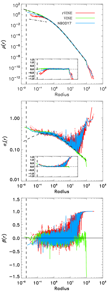
Figure 11: Radial profiles of the final density (upper panel), radial velocity dispersion (middle panel) and anisotropy parameter (bottom panel) for the models shown in Figure 9: B_Nbody7_100k (blue), B_Vine_100k (green) and B_rVine_100k (red lines). For comparison, the initial Hernquist profiles are shown with the dashed lines, the dashed-dotted line shows an inner density profile following $\rho\propto r^{-0.5}$, and the vertical dashed lines indicates the resolution limit in model B_Vine_100k, given as $\sim 2\,\epsilon_{\star}$. Inserts show the residuals from the initial Hernquist profiles for the same radial range. Shown are averages over several realisations of the initial conditions.

In Figure 11 we show the effect the ejection of low angular momentum stars at the bottom of the potential has on the structure of the galactic nucleus. Shown are radial profiles for the density (upper panel), the radial velocity dispersion (middle panel), and the velocity dispersion anisotropy parameter,

$$\beta_{\sigma}\equiv 1-\frac{\sigma_{\phi}^{2}+\sigma_{\theta}^{2}}{2\,\sigma_{\rm r}^{2}}$$ (14)

(bottom panel), for the models shown in Figure 9 at the end of the simulations. Stars are ejected from the galaxy centre by the hardening binary on orbits with high radial velocities in the B_rVine_100k (red) and B_Nbody7_100k (blue) runs. This leads to a large increase in the radial velocity dispersion at galacto-centric radii with $r\gtrsim 10\,r_{0}$ for these simulations (upper panel), together with a depression in the central density profile within $r\leq r_{\rm infl}^{\rm 2M}$ and some added mass in the outskirts of the galaxy (middle panel). The central density profile is converted from an initial Hernquist profile with inner slope of $\sim{-1}$ (dashed line) to a profile with $\rho\propto r^{-0.5}$ in the B_rVine_100k and B_Nbody7_100k runs. The increase in the radial velocity dispersion is not seen in the tangential velocity dispersions such that the anisotropy profile is strongly radially biased for $r\gtrsim 10\,r_{0}$. We verified that this is caused only by particles escaping the system after being ejected in interactions with the central binary in both codes. For B_Vine_100k (green), however, all radial profiles evolves insignificantly throughout the simulation. rVINE seems on average to be more effective in removing mass from the centre than NBODY7. Given that the SMBH binary hardens by roughly the same amount in both codes, this might be due to the fact that the central density is replenished more effectively by the high rate of collisional loss-cone refilling with stars originating from larger radii in the B_Nbody7_100k runs.

We further analyze the properties of the high radial velocity stars in the realisation using model B_rVine_100k shown in Figure 11 by examining the radial velocities of stars escaping the chain in Figure 12. Not all of the particles interacting with the SMBH binary leave the chain on high radial velocity orbits: the majority of the escapers has $v_{\rm rad}<1$ at all times in the simulation. However, for $t\lesssim 10$ there is an enhanced interaction rate of stars in the initially full loss-cone with the hardening SMBH binary leading to a significant population of escapers with radial velocities $1.5<v_{\rm rad}<2.5$, comparable to the expected kick velocities in a slingshot interaction of a field star with a massive binary with hardness $1/a\sim 1000$. Furthermore we find a small population of high-velocity outliers ($2<v_{\rm rad}<6.5$) - much higher than the expected kick velocity - which provide a clear observational signpost of the hard SMBH binary at the centre.

6 Discussion

Due to the favourable $\mathcal{O}(N\log(N))$ scaling of the tree code we should be able to employ (much) higher particle numbers than in the test calculations presented in this paper in future applications of the new code. However, as a caveat, we note that the time spent for the AR-chain calculations scales steeper with particle number than the time spent for the tree calculations, mostly due to the costly extrapolations of the Bulirsch-Stoer method and the repeated predictions and force evaluations of the perturbers. For the simulations performed for this paper execution of the chain part of the code has only taken a moderate fraction of the total CPU time (typically below $5\%$ with a maximum of $\sim 20\%$), and with some optimisation it should be possible to further increase the speed of the code. There will, however, be some critical particle number, $N_{\rm crit}$, at which the AR-chain will become the dominant contributor to the total computing costs even if only a small fraction of the total particle number is actually integrated in the chain. It is not within the scope of this paper to investigate this in detail and we leave this to future work where we will use our new hybrid code for full-scale galaxy simulations.

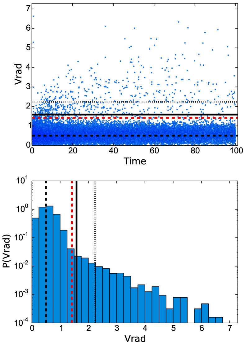
Figure 12: Radial velocity statistics of particles escaping the chain in one of the B_rVine_100k simulations, with $r_{\rm chain,0}=0.02$. Top panel: radial velocities as a function of time. bottom panel: Distribution of radial velocities of particles leaving the chain, with the velocities binned by $\Delta v=0.25$. For comparison we show the expected kick velocities ($v_{\rm kick}\propto\sqrt{G\,\mu/a}$, Saslaw et al., 1974) for inverse binary semi-major axes $1/a=100$ (dashed black line), $1/a=1000$ (solid black line) and $1/a=2000$ (dotted black line), and the escape velocity from the centre of a Hernquist sphere (dashed red line).

Throughout Section 5.2 we have found a qualitatively similar evolution of the hardening binary both in NBODY7 and rVINE for chain sizes of $\sim$ a few times the hard binary distance $a_{\rm hard}$ (Equation (13)). The agreement is particularly good for the highest particle numbers studied here ($N\geq 80k$) where spurious relaxation effects become less important in the direct N-body code. Similarly, for lower particle numbers ($N\leq 50k$), rVINE shows a shallower N-dependence of the hardening rate since the tree-code better reproduces the collisionless galactic stellar dynamics at distances far from the SMBHs. Hence, the hybrid code seems to catch the relevant dynamical interactions of a real galaxy better at lower $N$ for our set of parameters adopted for the chain.

However, we also note here that the high hardening rates we find in Section 5.2 in the NBODY7 simulations are somewhat larger than those found in a number of recent studies of spherical and axisymmetric models using similar techniques and initial conditions (see e.g. Khan et al., 2013; Vasiliev et al., 2014). In particular, the final binary hardness for our B_Nbody models are on average about a factor of $\sim 2.5$ higher for comparable particle numbers than the spherical models studied in Vasiliev et al. (2014). Several reasons could be responsible for this difference including slightly different choices in the initial positions and velocities of the SMBHs (see Section 5.2) or differences in the integration techniques (parameters for the AR-chain, settings for the gravitational softening and the integration accuracy, etc.), the most likely being the different way of introducing the SMBHs in the initial conditions. This may lead to an overestimate of the hardening rate, especially at the beginning of our simulations.

In Section 5.1 we have found that in the tree codes VINE and Gadget-3 — even with the most conservative choice of the SMBH softening length — the dynamical friction time-scales for the SMBH to sink to the galactic centre differ by more than $50\%$ from the ones in NBODY7 and rVINE. Hence are present-day cosmological and galaxy merger simulations suffering from significant (unavoidable) uncertainties in the SMBH orbital time-scales? Strictly speaking they do, but probably, in most cases SMBHs are rarely found orbiting ’naked’ in their host galaxies, but are instead embedded in stellar and gaseous cores or cusps that are then the prime subjects to dynamical friction in galaxy interactions. However, it has been shown that ’naked’ BHs might be quite commonly formed after the disruption of galactic nuclei in gas-rich minor mergers (Callegari et al., 2009; Van Wassenhove et al., 2014), making accurate estimates of the dynamical friction time-scales of the ’naked’ BHs necessary in these cases.

Of similar importance for the galaxy formation community is to get better estimates for SMBH binary coalescence time-scales in order to make robust predictions with respect to the dynamical evolution of SMBHs in their host galaxies. For example, studying the exciting possible formation of systems with multiple SMBHs at high redshift due to the high merger rate of galaxies relies crucially on (1) an accurate description of dynamical friction in order to correctly quantify the populations of binary, triple, etc. SMBHs being present at a given time, and (2) accurate orbits in order to reliably calculate the final outcome of the strong multi-body interactions between the SMBHs in the galactic centres (see e.g. Kulkarni & Loeb, 2012; Blecha et al., 2011). Obtaining accurate coalescence time-scales for binary SMBHs in gas-rich galaxy mergers is also essential for accurate estimates of the likelihood of recoiling SMBHs escaping from the rapidly steepening central potential of the merger remnants (e.g. Sijacki et al., 2011). This should be particularly relevant for large scale cosmological simulations like e.g. the recent EAGLE and Illustris (Schaye et al., 2015; Vogelsberger et al., 2014) simulations that assume fast coalescence of two SMBHs once their distance falls below the resolution limit (see e.g. Sijacki et al., 2014, for details).

7 Conclusions

In this paper we have presented a hybrid code combining an OpenMP-parallel binary tree code (VINE) with an algorithmic chain regularization scheme, and report on first tests with the new code called “rVINE”.

We have shown that, using the AR-regularized tree code, we can significantly improve the numerical accuracy in the calculation of the gravitational interactions of SMBHs with their close environment. By comparison with the collision-less code NBODY7, we have verified that we have overcome some of the fundamental limitations imposed by the gravitational softening of the SMBHs, as it is used in traditional tree codes. As a consequence, we are now able to follow the orbital evolution of SMBHs much more accurately in more realistic, galaxy-scale settings. We have shown that with the new hybrid code we obtain both significantly improved estimates for dynamical friction time-scales of single SMBHs sinking to the galactic centres and for the time evolution of hard SMBH binaries. In particular, using rVINE, we find a clear N-dependence of the binary hardening rate, a low binary eccentricity along with a moderate eccentricity evolution, as well as the conversion of the galaxy’s inner density profile from a cusp to a core via the ejection of low-angular momentum stars on orbits with high radial velocity, similar to the results obtained with NBODY7 here and in previous work.

Due to the modular design of rVine, the AR-chain part with its hybrid interface should be easily portable to other codes used for simulations of galaxy formation. It will likewise be straightforward to incorporate additional physics into rVine, e.g. formulations for hydrodynamics and additional sub-grid models of (1) star formation and stellar feedback, and (2) black hole accretion and feedback, or, the addition of post-Newtonian terms in the AR-chain. Note also that in the present paper we have restricted ourselves to the case of regularizing the dynamics of one single subsystem only. The next step here is to extend the present code to allow for multiple chains in order to handle the regularization of several distant SMBHs at once.

Important problems that will benefit from the accurate dynamical modelling of the evolution of (binary) SMBHs are predictions with regard to SMBH coalescence rates and their associated gravitational wave background (e.g. Haehnelt, 1994), the population of SMBHs and AGNs (either living at their host galaxies centres or being displaced from the central regions by three-body encounters or gravitational wave recoils), the acceleration of hyper-velocity stars (Hills, 1988), and the imprint of SMBH binaries on the structural and kinematic properties of the inner parts of the stellar component of galaxies (Ebisuzaki et al., 1991; Milosavljević & Merritt, 2001; Meiron & Laor, 2013).

Further improved hybrid codes like the one presented here will help to bridge the gap between different fields of astrophysics that are currently still separated by huge differences in the relevant scales of space, time, and mass and should eventually allow to study properly the effects of stellar dynamics in the sphere of influence of central supermassive black holes on the structure of their host galaxies.

References

- Aarseth (1963) Aarseth S. J., 1963, MNRAS, 126, 223
- Aarseth (1999) Aarseth S. J., 1999, PASP, 111, 1333
- Aarseth (2003a) Aarseth S. J., 2003a, Ap&SS, 285, 367
- Aarseth (2003b) Aarseth S. J., 2003b, Gravitational N-Body Simulations
- Aarseth (2007) Aarseth S. J., 2007, MNRAS, 378, 285
- Barnes & Hut (1986) Barnes J., Hut P., 1986, Nature, 324, 446
- Bédorf et al. (2012) Bédorf J., Gaburov E., Portegies Zwart S., 2012, Journal of Computational Physics, 231, 2825
- Berczik et al. (2006) Berczik P., Merritt D., Spurzem R., Bischof H.-P., 2006, ApJ, 642, L21
- Berczik et al. (2013) Berczik P., Spurzem R., Wang L., 2013, in Third International Conference ”High Performance Computing”, HPC-UA 2013, p. 52-59, pp. 52–59
- Binney & Tremaine (2008) Binney J., Tremaine S., 2008, Galactic Dynamics: Second Edition, Binney, J. & Tremaine, S., ed. Princeton University Press
- Blecha et al. (2011) Blecha L., Cox T. J., Loeb A., Hernquist L., 2011, MNRAS, 412, 2154
- Booth & Schaye (2009) Booth C. M., Schaye J., 2009, MNRAS, 398, 53
- Bulirsch & Stoer (1966) Bulirsch R., Stoer J., 1966, Numerische Mathematik, 8, 1
- Callegari et al. (2009) Callegari S., Mayer L., Kazantzidis S., Colpi M., Governato F., Quinn T., Wadsley J., 2009, ApJ, 696, L89
- Chandrasekhar (1943) Chandrasekhar S., 1943, ApJ, 97, 255
- Choi et al. (2012) Choi E., Ostriker J. P., Naab T., Johansson P. H., 2012, ApJ, 754, 125
- Civano et al. (2011) Civano F. et al., 2011, ApJ, 741, 91
- Dehnen (1993) Dehnen W., 1993, MNRAS, 265, 250
- Di Matteo et al. (2008) Di Matteo T., Colberg J., Springel V., Hernquist L., Sijacki D., 2008, ApJ, 676, 33
- Ebisuzaki et al. (1991) Ebisuzaki T., Makino J., Okumura S. K., 1991, Nature, 354, 212
- Fan et al. (2001) Fan X. et al., 2001, AJ, 122, 2833
- Ferrarese & Merritt (2000) Ferrarese L., Merritt D., 2000, ApJ, 539, L9
- Fujii et al. (2007) Fujii M., Iwasawa M., Funato Y., Makino J., 2007, PASJ, 59, 1095
- Gaburov et al. (2009) Gaburov E., Harfst S., Portegies Zwart S., 2009, NewA, 14, 630
- Gebhardt et al. (2000) Gebhardt K. et al., 2000, ApJ, 539, L13
- Gragg (1965) Gragg W., 1965, Journal of the Society for Industrial and Applied Mathematics: Series B, Numerical Analysis, 2, 384
- Haehnelt (1994) Haehnelt M. G., 1994, MNRAS, 269, 199
- Harfst et al. (2008) Harfst S., Gualandris A., Merritt D., Mikkola S., 2008, MNRAS, 389, 2
- Häring & Rix (2004) Häring N., Rix H.-W., 2004, ApJ, 604, L89
- Hellström & Mikkola (2010) Hellström C., Mikkola S., 2010, Celestial Mechanics and Dynamical Astronomy, 106, 143
- Hernquist (1990) Hernquist L., 1990, ApJ, 356, 359
- Hills (1988) Hills J. G., 1988, Nature, 331, 687
- Hut et al. (2010) Hut P., McMillan S., Makino J., Portegies Zwart S., 2010, Starlab: A Software Environment for Collisional Stellar Dynamics. Astrophysics Source Code Library
- Johansson et al. (2009) Johansson P. H., Naab T., Burkert A., 2009, ApJ, 690, 802
- Just et al. (2011) Just A., Khan F. M., Berczik P., Ernst A., Spurzem R., 2011, MNRAS, 411, 653
- Just & Peñarrubia (2005) Just A., Peñarrubia J., 2005, A&A, 431, 861
- Kauffmann & Haehnelt (2000) Kauffmann G., Haehnelt M., 2000, MNRAS, 311, 576
- Khan et al. (2013) Khan F. M., Holley-Bockelmann K., Berczik P., Just A., 2013, ApJ, 773, 100
- Khan et al. (2011) Khan F. M., Just A., Merritt D., 2011, ApJ, 732, 89
- Khan et al. (2012) Khan F. M., Preto M., Berczik P., Berentzen I., Just A., Spurzem R., 2012, ApJ, 749, 147
- Kormendy & Ho (2013) Kormendy J., Ho L. C., 2013, ARA&A, 51, 511
- Kormendy & Richstone (1995) Kormendy J., Richstone D., 1995, ARA&A, 33, 581
- Kravtsov et al. (1997) Kravtsov A. V., Klypin A. A., Khokhlov A. M., 1997, ApJS, 111, 73
- Kulkarni & Loeb (2012) Kulkarni G., Loeb A., 2012, MNRAS, 422, 1306
- Kustaanheimo & Stiefel (1965) Kustaanheimo P., Stiefel E., 1965, J. Reine Angew. Math., 218, 204
- Lodato et al. (2009) Lodato G., King A. R., Pringle J. E., 2009, MNRAS, 392, 332
- Lynden-Bell (1969) Lynden-Bell D., 1969, Nature, 223, 690
- Magorrian et al. (1998) Magorrian J. et al., 1998, AJ, 115, 2285
- Martizzi et al. (2012) Martizzi D., Teyssier R., Moore B., 2012, MNRAS, 420, 2859
- McMillan & Aarseth (1993) McMillan S. L. W., Aarseth S. J., 1993, ApJ, 414, 200
- Meiron & Laor (2013) Meiron Y., Laor A., 2013, MNRAS, 433, 2502
- Merritt et al. (2007) Merritt D., Mikkola S., Szell A., 2007, ApJ, 671, 53
- Mikkola & Aarseth (2002) Mikkola S., Aarseth S., 2002, Celestial Mechanics and Dynamical Astronomy, 84, 343
- Mikkola & Aarseth (1990) Mikkola S., Aarseth S. J., 1990, Celestial Mechanics and Dynamical Astronomy, 47, 375
- Mikkola & Aarseth (1993) Mikkola S., Aarseth S. J., 1993, Celestial Mechanics and Dynamical Astronomy, 57, 439
- Mikkola & Merritt (2006) Mikkola S., Merritt D., 2006, MNRAS, 372, 219
- Mikkola & Tanikawa (1999a) Mikkola S., Tanikawa K., 1999a, MNRAS, 310, 745
- Mikkola & Tanikawa (1999b) Mikkola S., Tanikawa K., 1999b, Celestial Mechanics and Dynamical Astronomy, 74, 287
- Milosavljević & Merritt (2001) Milosavljević M., Merritt D., 2001, ApJ, 563, 34
- Milosavljević & Merritt (2003) Milosavljević M., Merritt D., 2003, ApJ, 596, 860
- Mortlock et al. (2011) Mortlock D. J. et al., 2011, Nature, 474, 616
- Nelson et al. (2009) Nelson A. F., Wetzstein M., Naab T., 2009, ApJS, 184, 326
- Nitadori & Aarseth (2012) Nitadori K., Aarseth S. J., 2012, MNRAS, 424, 545
- Portegies Zwart et al. (2009) Portegies Zwart S. et al., 2009, NewA, 14, 369
- Portegies Zwart et al. (2013) Portegies Zwart S., McMillan S. L. W., van Elteren E., Pelupessy I., de Vries N., 2013, Computer Physics Communications, 183, 456
- Preto et al. (2011) Preto M., Berentzen I., Berczik P., Spurzem R., 2011, ApJ, 732, L26+
- Preto & Tremaine (1999) Preto M., Tremaine S., 1999, AJ, 118, 2532
- Pretorius (2005) Pretorius F., 2005, Physical Review Letters, 95, 121101
- Rees (1984) Rees M. J., 1984, ARA&A, 22, 471
- Richstone et al. (1998) Richstone D. et al., 1998, Nature, 395, A14+
- Saslaw et al. (1974) Saslaw W. C., Valtonen M. J., Aarseth S. J., 1974, ApJ, 190, 253
- Schaye et al. (2015) Schaye J. et al., 2015, MNRAS, 446, 521
- Sijacki et al. (2011) Sijacki D., Springel V., Haehnelt M. G., 2011, MNRAS, 414, 3656
- Sijacki et al. (2014) Sijacki D., Vogelsberger M., Genel S., Springel V., Torrey P., Snyder G., Nelson D., Hernquist L., 2014, preprint (arXiv:1408.6842)
- Silk & Rees (1998) Silk J., Rees M. J., 1998, A&A, 331, L1
- Springel (2005) Springel V., 2005, MNRAS, 364, 1105
- Springel (2010) Springel V., 2010, MNRAS, 401, 791
- Springel et al. (2005) Springel V., Di Matteo T., Hernquist L., 2005, MNRAS, 361, 776
- Teyssier (2002) Teyssier R., 2002, A&A, 385, 337
- Tremaine et al. (2002) Tremaine S. et al., 2002, ApJ, 574, 740
- Tremaine et al. (1994) Tremaine S., Richstone D. O., Byun Y.-I., Dressler A., Faber S. M., Grillmair C., Kormendy J., Lauer T. R., 1994, AJ, 107, 634
- Van Wassenhove et al. (2014) Van Wassenhove S., Capelo P. R., Volonteri M., Dotti M., Bellovary J. M., Mayer L., Governato F., 2014, MNRAS, 439, 474
- Vasiliev et al. (2014) Vasiliev E., Antonini F., Merritt D., 2014, ApJ, 785, 163
- Vogelsberger et al. (2014) Vogelsberger M. et al., 2014, MNRAS, 444, 1518
- Wadsley et al. (2004) Wadsley J. W., Stadel J., Quinn T., 2004, NewA, 9, 137
- Wang et al. (2015) Wang L., Spurzem R., Aarseth S., Nitadori K., Berczik P., Kouwenhoven M. B. N., Naab T., 2015, preprint (arXiv:1504.03687)
- Wetzstein et al. (2009) Wetzstein M., Nelson A. F., Naab T., Burkert A., 2009, ApJS, 184, 298
- White (1976) White S. D. M., 1976, MNRAS, 174, 467
- Wisdom & Holman (1991) Wisdom J., Holman M., 1991, AJ, 102, 1528
- Zare (1974) Zare K., 1974, Celestial Mechanics, 10, 207