Stroboscopic prethermalization in weakly interacting periodically driven systems

Abstract

Time-periodic driving provides a promising route to engineer non-trivial states in quantum many-body systems. However, while it has been shown that the dynamics of integrable, non-interacting systems can synchronize with the driving into a non-trivial periodic motion, generic non-integrable systems are expected to heat up until they display a trivial infinite-temperature behavior. In this paper we show that a quasi-periodic time evolution over many periods can also emerge in weakly interacting systems, with a clear separation of the timescales for synchronization and the eventual approach of the infinite-temperature state. This behavior is the analogue of prethermalization in quenched systems. The synchronized state can be described using a macroscopic number of approximate constants of motion. We corroborate these findings with numerical simulations for the driven Hubbard model.

I Introduction

Experiments with ultra-cold atomic gases in optical lattices and ultra-fast spectroscopy nowadays allow to address the dynamics of quantum many-particle systems out of equilibrium. A particularly important role in this context is played by periodically driven systems Shirley (1965); Sambe (1973); Breuer, H.P., Dietz, K., and Holthaus, M. (1990); Grifoni and Hänggi (1998). Periodic driving can stabilize novel states both in cold atoms and in condensed matter, including topologically nontrivial states Oka and Aoki (2009); Kitagawa et al. (2011); Iadecola et al. (2013); Kitagawa et al. (2010); Lindner, Refael, and Galitski (2011); Wang et al. (2013) or complex phases such as superconductivity Fausti et al. (2011); Hu et al. (2014). It can be used to engineer artificial gauge fields in cold atoms Goldman and Dalibard (2014) and emergent many-body interactions such as magnetic exchange interactions in solids Mentink, Balzer, and Eckstein (2015); Mikhaylovskiy et al. ; Itin and Katsnelson , or to transiently modify lattice structures through anharmonic couplings Först et al. (2011).

An important question is thus the theoretical understanding of the long-time dynamics of periodically driven systems. The approach to a steady state has been investigated intensively for the relaxation of isolated systems after a sudden perturbation, both experimentally and theoretically Polkovnikov et al. (2011); Kinoshita, Wenger, and Weiss (2006); Trotzky et al. (2012). When a generic non-integrable many-body system is left to evolve with a time-independent Hamiltonian, it is believed to eventually relax to a thermal equilibrium state, unless it is in a many-body localized phase Altshuler et al. (1997); Gornyi, Mirlin, and Polyakov (2005); Basko, Aleiner, and Altshuler (2006). If the system is integrable, on the other hand, the steady state is often described by a generalized Gibbs ensemble (GGE) Rigol et al. (2007); Langen et al. (2015), which keeps track of a macroscopic number of constants of motion. When integrability is only slightly broken, the system can display dynamics on separate timescales, such that observables rapidly prethermalize to a quasi-steady nonequilibrium state which can be understood by a GGE based on perturbatively constructed constants of motion Kollar, Wolf, and Eckstein (2011), before thermalizing on much longer time scales Berges, Borsányi, and Wetterich (2004); Moeckel and Kehrein (2008); Gring et al. (2012).

Integrability turns out to be a crucial factor also for periodically driven systems. Their dynamics can synchronize with the driving Russomanno, Silva, and Santoro (2012) and display a non-trivial periodic time evolution at long times. A way to understand this is to show that the time evolution over one period $T$ commutes with an infinite number of operators $\mathcal{I}_{\lambda}$, which are thus conserved at stroboscopic times (i.e. integer multiples of the period). Having a fixed expectation value of all $\mathcal{I}_{\lambda}$ at stroboscopic times, one can construct a statistical ensemble to describe the long-time behavior of the system (the periodic Gibbs ensemble), which has been analytically and numerically shown to give correct predictions for hard-core bosons Lazarides, Das, and Moessner (2014a).

In contrast to integrable systems (and many-body localized states Lazarides, Das, and Moessner (2015); Abanin, De Roeck, and Huveneers (2014); D’Alessio and Polkovnikov (2013); Ponte et al. (2015a, b); Roy and Das (2015)), it has been proposed that generic non-integrable systems “heat up” under the effect of driving and display rather trivial infinite temperature properties as soon as they settle into a periodic motion Lazarides, Das, and Moessner (2014b); D’Alessio and Rigol (2014); Eckardt and Anisimovas . One can formulate this statement in terms of the Floquet eigenstates (the exact solutions of the Schrödinger equation with a periodic evolution of all observables Dittrich et al. (1998); Grifoni and Hänggi (1998)), stating that each individual Floquet state displays infinite temperature properties. This conjecture relies on a breakdown of the perturbative expansion of Floquet eigenstates at some order because of unavoidable resonances between transitions in the many-body spectrum with multiples of the driving frequency. A common approach to avoid this problem is to construct effective Floquet Hamiltonians from a high-frequency expansion D’Alessio and Polkovnikov (2013); Goldman and Dalibard (2014). In this work we show that a quasi-periodic state can also emerge in weakly interacting systems, provided that linear absorption can be avoided: the stroboscopic time evolution is constrained by approximately conserved constants of motion $\tilde{\mathcal{I}}_{\lambda}$. Analogously to prethermalization in weakly interacting systems after a sudden perturbation Berges, Borsányi, and Wetterich (2004); Moeckel and Kehrein (2008); Kollar, Wolf, and Eckstein (2011), the system rapidly synchronizes with the driving and remains periodic over a large number of periods $m$ such that $g^{-1}\gg mT\gg J^{-1}$, where $g$ controls the strength of the interaction, $T$ is the period of the driving and $J$ is coupling of the integrable Hamiltonian, e.g., the bandwidth of the kinetic energy term; we set $\hbar$ $=$ $1$ throughout. The quasi-periodic state can be described as a periodic Gibbs ensemble based on the $\tilde{\mathcal{I}}_{\lambda}$, i.e., stroboscopic prethermalization gives access to quasi-periodic states which are entirely different from the infinite temperature final states.

This paper is organized as follows: in Sec. II we introduce the general formalism: first, we rotate the weakly interacting Hamiltonian in such a way that it commutes with the integrals of motion of the noninteracting part (Sec. II.1), then in Sec. II.2 we identify the approximate integrals of motion and finally in Sec. II.3 study the time evolution of the observables. In Sec. III we discuss the relation with the periodic Gibbs ensemble Lazarides, Das, and Moessner (2014a) and in Sec. IV the relation with the Floquet theory of periodically driven systems. In Sec. V we specialize the results of Sec. II to the Hubbard model, first presenting our analytical results (Sec. V.1) and then comparing them to the numerical findings (Sec. V.2) obtained with dynamical mean-field theory. In Sec. VI we draw our conclusions.

II General formalism

In the following we consider an integrable, noninteracting system perturbed by a weak periodic interaction. The general Hamiltonian is given by

$$H(t)=H_{0}+gH_{\rm int}(t),$$ (1)

where the integrable part

$$H_{0}=\sum_{\lambda}\epsilon_{\lambda}\hat{\mathcal{I}}_{\lambda}\;,$$ (2)

can be written as a sum of constants of motion (e.g., momentum occupations for independent particles on a lattice), and the small parameter $g$ controls the strength of the interaction $H_{\rm int}(t)$ which is periodic with period $T$ and frequency $\Omega=2\pi/T$. To study the time evolution at stroboscopic times $t_{m}=mT$ ($m$ integer), we extend the approach of Refs. Kollar, Wolf, and Eckstein (2011); Moeckel and Kehrein (2008) to periodically driven systems, and determine a time-periodic unitary transformation $R(t)$ such that the Hamiltonian $H_{\rm eff}(t)$ in the rotated frame commutes with the constants of motion $\hat{\mathcal{I}}_{\lambda}$ at any time up to corrections or order $\mathcal{O}(g^{3})$ . If $|\tilde{\psi}(t)\rangle=R(t)|\psi(t)\rangle$ is the transformed wave function, the Hamiltonian $H_{\rm eff}$ which dictates the evolution in the rotated frame via $i\partial_{t}|\tilde{\psi}(t)\rangle=H_{\rm eff}(t)|\tilde{\psi}(t)\rangle$ is given by

$$\begin{split}H_{\rm eff}(t)&=R(t)H(t)R(t)^{\dagger}-iR(t)\dot{R}(t)^{\dagger}\;.\end{split}$$ (3)

Since $R(t)$ is assumed to be unitary, we make the ansatz $R(t)\equiv e^{S(t)}$, with an anti-hermitian operator $S(t)$.

In the next sections, we first analytically find the transformation $S(t)$ (Sec. II.1), then identify the approximate integrals of motion (Sec. II.2) and finally in Sec. II.3 we study the time evolution of the expectation values of observables and the dependence of their long-time behavior on the frequency $\Omega$.

II.1 The transformation $S(t)$

We now show in detail how to rotate the Hamiltonian Eq. (1) with a transformation $R(t)$ $=$ $e^{S(t)}$ such that the Hamiltonian (3) is (i) periodic and (ii) diagonal in the operators that diagonalize $H_{0}$. To implement condition (i), we first expand to second order in $g$ and then write in Fourier series both the effective Hamiltonian

$$\begin{split}H_{\rm eff}(t)&=H_{\rm eff}^{(0)}(t)+gH_{\rm eff}^{(1)}(t)+g^{2}H_{\rm eff}^{(2)}(t)\\ &=\sum_{n}e^{-in\Omega t}\left[H_{\rm eff,n}^{(0)}+gH_{\rm eff,n}^{(1)}+g^{2}H_{\rm eff,n}^{(2)}\right]\end{split}$$ (4)

and the anti-hermitian operator

$$\begin{split}S(t)&=gS^{(1)}(t)+\frac{g^{2}}{2}S^{(2)}(t)+\mathcal{O}(g^{3})\\ &=\sum_{n}e^{-in\Omega t}[gS^{(1)}_{n}+\frac{g^{2}}{2}S^{(2)}_{n}]+\mathcal{O}(g^{3})\;,\end{split}$$ (5)

with $H_{{\rm eff},n}=H_{{\rm eff},-n}^{\dagger}$ and $S_{n}=-S_{-n}^{\dagger}$. Combining Eqs. (3) and (4) we find:

$$\begin{split}&H_{\rm eff}(t)=H_{0}+g\left(H_{\rm int}(t)+[S^{(1)}(t),H_{0}]+i\frac{d}{dt}S^{(1)}(t)\right)\\ &+g^{2}\left(\frac{1}{2}[S^{(2)}(t),H_{0}]+[S^{(1)}(t),H_{\rm int}(t)]+\right.\\ &\frac{1}{2}[S^{(1)}(t),[S^{(1)}(t),H_{0}]]+\frac{i}{2}\frac{d}{dt}S^{(2)}(t)+\\ &\left.-\frac{i}{2}(\dot{S}^{(1)}(t)S^{(1)}(t)-S^{(1)}(t)\dot{S}^{(1)}(t))\right)+\mathcal{O}(g^{3})\;.\end{split}$$ (6)

To ensure condition (ii), we require that

$$[H_{\rm eff,n}^{(X)},\hat{\mathcal{I}}_{\lambda}]=0,$$ (7)

for any Fourier component, perturbative order and constant of motion, labeled by $n$, $X$ and $\lambda$ respectively. As in Ref. Kollar, Wolf, and Eckstein, 2011, we employ the basis $\hat{\mathcal{I}}_{\lambda}|\bm{\alpha}\rangle=\alpha_{\lambda}|\bm{\alpha}\rangle$. We assume that the energies $\epsilon_{\lambda}$ are incommensurate, so that the eigenenergies of $H_{0}$, i.e. $E_{\bm{\alpha}}=\sum_{\lambda}\epsilon_{\lambda}\alpha_{\lambda}$, are nondegenerate. For an extensive lattice model this can be achieved, e.g., by using sufficiently irregular boundaries.

After some lengthy but otherwise straightforward algebra, we can find $H_{\rm eff}(t)$ and $S(t)$ by repeatedly applying Eq. (7) to each perturbative order in Eq. (6), so as to reduce the Hamiltonian to the diagonal form

$$H_{\rm eff}(t)=H_{0}+\sum_{\alpha}|\alpha\rangle E_{\rm diag,\alpha}(t)\langle\alpha|+\mathcal{O}(g^{3})\;.$$ (8)

In order $g^{0}$ we have

$$H_{\rm eff,n}^{(0)}=\left\{\begin{array}[]{ll}H_{0}&\qquad{\rm if}\;n=0\\ 0&\qquad{\rm otherwise}\;,\end{array}\right.$$ (9)

so that $H_{\rm eff,0}^{(0)}=\sum_{\alpha}|\alpha\rangle\langle\alpha|E^{(0)}_{0,\alpha}$, with $E^{(0)}_{0,\alpha}=E_{\alpha}$.

To first order in $g$ the Fourier components of $S(t)$ read:

$$\langle\beta|S_{n}^{(1)}|\alpha\rangle=\left\{\begin{array}[]{ll}\frac{\langle\beta|{H_{\rm int,n}}|\alpha\rangle}{E_{\beta}-E_{\alpha}-n\Omega}&{\rm if}\quad\alpha\neq\beta\\ 0&\qquad{\rm otherwise}\end{array}\right.$$ (10)

The first-order perturbative correction to $H_{\rm eff}$ is:

$$\begin{split}H_{\rm eff}^{(1)}(t)&=\sum_{\alpha}e^{-in\Omega t}|\alpha\rangle E^{(1)}_{n,\alpha}\langle\alpha|\end{split}$$ (11)

where

$$E^{(1)}_{n,\alpha}=\langle\alpha|H_{\rm int,n}|\alpha\rangle\;.$$ (12)

At order $g^{2}$ the Fourier components of $S^{(2)}$ are found to be:

$$\langle\beta|S^{(2)}_{n}|\alpha\rangle=\sum_{p}\frac{\langle\beta|\left[S_{p}^{(1)},H_{{\rm int},n-p}+H^{(1)}_{{\rm diag},n-p}\right]|\alpha\rangle}{E_{\beta}-E_{\alpha}-n\Omega}$$ (13)

if $\alpha\neq\beta$ and, as previously, we choose the diagonal elements to be zero. In Eq. (13) we have defined: $H^{(1)}_{{\rm diag},n}=\sum_{\alpha}|\alpha\rangle E^{(1)}_{n,\alpha}\langle\alpha|$. Finally, the second order term of the effective Hamiltonian reads:

$$H^{(2)}_{{\rm eff},n}=\sum_{\alpha}|\alpha\rangle E^{(2)}_{n,\alpha}\langle\alpha|\;,$$ (14)

with:

$$\begin{split}E^{(2)}_{n,\alpha}=&\frac{1}{2}\sum_{\beta\neq\alpha}\sum_{p}\left[\frac{\langle\alpha|H_{{\rm int},p}|\beta\rangle\langle\beta|H_{{\rm int},n-p}|\alpha\rangle}{E_{\alpha}-E_{\beta}-p\Omega}\right.\\ &-\left.\frac{\langle\alpha|H_{{\rm int},n-p}|\beta\rangle\langle\beta|H_{{\rm int},p}|\alpha\rangle}{E_{\beta}-E_{\alpha}-p\Omega}\right]\;.\end{split}$$ (15)

II.2 Approximate integrals of motion

Under a general unitary transformation, the time propagator $U(t,0)$ $=$ $\mathcal{T}e^{-i\int_{0}^{t}dt^{\prime}\,H(t^{\prime})}$ is transformed into

$$U(t,0)=e^{-S(t)}\,\tilde{U}(t,0)\,e^{S(0)},$$ (16)

with $\tilde{U}(t,0)$ $=$ $\mathcal{T}e^{-i\int_{0}^{t}dt^{\prime}\,H_{\rm eff}(t^{\prime})}$. Because $S(t)$ is periodic, the time evolution at stroboscopic times is thus unitarily equivalent to the time evolution with the diagonal Hamiltonian (8), $U(t_{m},0)=e^{-S(0)}e^{-i\int_{0}^{t_{m}}dt\,H_{\rm eff}(t)}e^{S(0)}+t_{m}\mathcal{O}(g^{3})$. This implies that the quantities

$$\tilde{\mathcal{I}}_{\lambda}=e^{-S(0)}\hat{\mathcal{I}}_{\lambda}e^{S(0)}$$ (17)

are approximately conserved under the evolution over multiple periods $T$, i.e., $\langle\tilde{\mathcal{I}}_{\lambda}(t_{m})\rangle=\langle\tilde{\mathcal{I}}_{\lambda}(0)\rangle+t_{m}\mathcal{O}(g^{3})$. For the example of a weakly interacting Hubbard model studied below, the original constants of motion are momentum occupations $n_{{\bm{k}}}$ of independent particles, while the constants of motion of the stroboscopic time evolution correspond to quasiparticle modes.

II.3 Expectation value of observables

We examine the synchronization of these modes in terms of the time evolution

$$\langle A\rangle_{t}\equiv\langle\psi(0)|U^{\dagger}(t,0)AU(t,0)|\psi(0)\rangle\;$$ (18)

of an observable $\hat{A}$ which is a function of the original constants of motion $\mathcal{I}_{\lambda}$ (having in mind, e.g., a measurement of momentum occupations $n_{{\bm{k}}}$ or higher-order momentum correlation functions $n_{{\bm{k}}}n_{{\bm{k^{\prime}}}}$), assuming that the system is in an eigenstate $|\psi(0)\rangle\equiv|\alpha\rangle$ of $H_{0}$ before the driving is switched on. Inserting Eq. (16) into (18), expanding the operators $e^{S(0)}$ and $e^{S(t)}$ in powers of $g$, and using the fact that $[A,\tilde{U}(t,0)]=t\mathcal{O}(g^{3})$ (because $A$ commutes with all $\mathcal{I}_{\lambda}$), we obtain

$$\langle A\rangle_{t}=-2{\rm Re}\langle\alpha|S(0)A[S(0)-\bar{S}(t)]|\alpha\rangle+t\mathcal{O}(g^{3}),$$ (19)

with $\bar{S}(t)\equiv\tilde{U}^{\dagger}(t,0)S(t)\tilde{U}(t,0)\;$. For stroboscopic times, with $S(t_{m})=S(0)$ determined by Eq. (10), one finds the final result for the perturbative time evolution

$$\!\!\!\langle A\rangle_{t_{m}}=\sum_{n,p}\int\limits_{-\infty}^{\infty}\!\!d\omega\,\frac{4g^{2}\sin^{2}(\frac{\omega t_{m}}{2})y_{np}(\omega)}{(\omega-n\Omega)(\omega-p\Omega)}+t_{m}\mathcal{O}(g^{3}),$$ (20)

where $y_{np}(\omega)$ denotes the spectral density

$$\begin{split}y_{np}(\omega)=&\langle\alpha|H_{{\rm int},-n}A\delta(\omega-H_{0}+E_{\alpha})H_{{\rm int},-p}|\alpha\rangle\;.\end{split}$$ (21)

The integral in Eq. (20) gives an accurate description of $\langle A\rangle_{t_{m}}$ for times $t_{m}\ll g^{-1}$, where relative corrections $t_{m}\mathcal{O}(g^{3})$ are small. Note that for finite $m$ the term $\sin(t_{m}\omega/2)$ regularizes the singularities at $n\omega$. Therefore the amount of contributing spectral weight is due to the location of $\Omega$ inside or outside the band, as discussed below. For $g\to 0$ there is thus a large time window $g^{-1}\gg t_{m}\gg T$ in which the dynamics is governed by the long time asymptotics of the integral. To analyze this, we distinguish two different behaviors depending on the frequency $\Omega$:

(i) Fermi golden rule regime: If there is nonzero spectral density $y_{nn}(n\Omega)>0$ at an even pole $1/(\omega-n\Omega)^{2}$, the stroboscopic evolution for $m\gg 1$ develops a linear asymptotics $\langle A\rangle_{t_{m}}\sim g^{2}t_{m}\sum_{\beta\neq\alpha}\langle\beta|A|\beta\rangle\Gamma_{\alpha\to\beta}$, where $\Gamma_{\alpha\to\beta}$ is the Fermi golden rule excitation rate

$$\Gamma_{\alpha\to\beta}=2\pi\sum_{n}|\langle\beta|H_{\rm int,n}|\alpha\rangle|^{2}\delta(n\Omega-E_{\beta}+E_{\alpha}).$$ (22)

To see this fact one can consider the contribution to the integral (20) from a small interval $|\omega-n\Omega|\leq\epsilon$ around the pole, in which $y_{nn}(\omega)$ can be approximated by a constant $y_{nn}(n\Omega)$. With a substitution $x=t_{m}(\omega-n\Omega)$, the remaining integral is $t_{m}\int_{-\epsilon t_{m}}^{\epsilon t_{m}}dx\,\sin^{2}(x/2)/x^{2}\sim t_{m}\pi/2$. From a similar consideration for $n$ $\neq$ $p$ one can obtain the subleading terms.

(ii) Stroboscopic prethermalization: Assuming that the perturbation involves only a limited number of Fourier components, such as for a harmonic perturbation with $H_{{\rm int},n}=0$ for $|n|>1$, then the spectral density $y_{nm}(\omega)$ is restricted to a finite band $[-W,W]$, depending on the type of excitation, the bandwidth of the noninteracting single-particle spectrum, and phase space restrictions. If all poles $\omega=n\Omega$ lie outside this band, the limit $m\to\infty$ integral of (20) is simply obtained by replacing $\sin^{2}(t_{m}\omega/2)$ by its average $1/2$, which corresponds to the first term in Eq. (19),

$$\langle A\rangle_{\text{pre}} =-2{\rm Re}\langle\alpha|S(0)AS(0)|\alpha\rangle$$

$$=2g^{2}\sum_{n,p}\int_{-\infty}^{\infty}\!\!d\omega\,\frac{y_{np}(\omega)}{(\omega-n\Omega)(\omega-p\Omega)}\;.$$ (23)

In this case the system synchronizes for $t_{m}\gg T$ (and $t_{m}\ll g^{-1}$) into a periodic evolution with values $\langle A\rangle_{t_{m}}=\langle A\rangle_{\text{pre}}$, before further heating takes place on longer timescales. This is the analogue of prethermalization in a quenched system.

III Statistical description of the prethermalized state

The condition $y_{nn}(n\Omega)=0$ for the absence of linear absorption is equivalent to the absence of resonances in Eq. (10). Outside the Fermi golden rule regime, the constants of motion (17) are thus well-defined, and one can ask whether the prethermalized state can be described by a Gibbs ensemble $\rho_{\tilde{G}}=\sum_{\lambda}e^{-\mu_{\lambda}\tilde{\mathcal{I}}_{\lambda}}/Z_{\tilde{G}}$ , where the Lagrange multipliers $\mu_{\lambda}$ are determined by the constraint from the initial state, $\langle\tilde{\mathcal{I}}_{\lambda}\rangle_{0}=\text{tr}\big{[}\rho_{\tilde{G}}\tilde{\mathcal{I}}_{\lambda}]$,

$$\langle A\rangle_{\text{pre}}=\text{tr}\big{[}\rho_{\tilde{G}}A].$$ (24)

Using Eqs. (II.3) and (17), the proof for this statement only relies on the time-independent matrix $S(0)$ being antihermitian and appearing only to order $g$ in $\text{tr}\big{[}\rho_{\tilde{G}}A]$, and thus proceeds analogously to the argument showing that prethermalized states for a sudden quench can be described by a GGE Kollar, Wolf, and Eckstein (2011).

IV Relation to the Floquet picture

We now explain how the prethermalized state Eq. (II.3) can be related to the Floquet spectrum of the Hamiltonian. According to the Floquet theorem, the exact solution of the Schrödinger equation with a time-periodic Hamiltonian (1) is given in the form $|\psi_{F,\alpha}(t)\rangle=e^{-iE_{F,\alpha}t}|\psi_{\alpha}(t)\rangle$, where $|\psi_{\alpha}(t)\rangle$ is periodic in time. If a system is in a Floquet state, the time evolution of observables is periodic. By expanding $|\psi_{\alpha}(t)\rangle$ in a Fourier series $|\psi_{\alpha}(t)\rangle=\sum_{m}e^{-i\Omega mt}|\psi_{\alpha,m}\rangle$, the Floquet quasi-energy spectrum can be obtained by diagonalizing the time-independent block-matrix,

$$(E_{F,\alpha}+m\Omega-H_{0})|\psi_{\alpha,m}\rangle=g\sum_{l}H_{{\rm int},l}|\psi_{\alpha,m+l}\rangle.$$ (25)

In principle, one can now use standard first-order perturbation theory to construct perturbative Floquet states $|\psi_{\alpha,n}\rangle=|\psi_{\alpha,n}^{(0)}\rangle+g|\psi_{\alpha,n}^{(1)}\rangle+\cdots$, where the zeroth order is given by the unperturbed eigenstates $|\psi_{\alpha,m}^{(0)}\rangle=\delta_{m,0}|\alpha\rangle$ ($E_{F,\alpha}^{(0)}=E_{\alpha}$). The perturbative expansion does not converge to the true Floquet eigenstate if there are resonances $E_{\alpha}-E_{\beta}=n\Omega$ in the many-body spectrum, but low orders nevertheless can exist: in particular, the first order is given by $|\psi_{\alpha,m}^{(1)}\rangle=S_{m}^{(1)}|\alpha\rangle$, and it is well-defined outside the Fermi golden rule regime. This shows that the prethermalized state Eq. (II.3) is related to the perturbative Floquet state by

$$\langle A\rangle_{\text{pre}}=2\langle\psi_{F,\alpha}^{(1)}|A|\psi_{F,\alpha}^{(1)}\rangle.$$ (26)

Here the appearance of a factor of two is reminiscent to a similar relation between the prethermalized and ground state expectation values in the quench case.

V Application to the Hubbard model in infinite dimensions

V.1 Analytical results

In order to illustrate the general results above, we now choose as specific example the Hubbard model

$$H(t)=-J\sum_{\langle ij\rangle\sigma}c^{\dagger}_{i\sigma}c_{j\sigma}+U(t)\sum_{i}(n_{i\uparrow}-\tfrac{1}{2})(n_{i\downarrow}-\tfrac{1}{2})\,,$$ (27)

with nearest neighbor hopping $J$ and periodically modulated interaction

$$U(t)=U(1-\cos(\Omega t))\,.$$ (28)

With these choices, the first and the second term of Eq. (27) represent the integrable, noninteracting part $H_{0}$ and the periodic weakly interacting perturbation with $g=U$, respectively. Energy and time are measured in units of $J$ and $J^{-1}$, respectively. The constants of motion of $H_{0}$ are momentum occupation numbers $\hat{n}_{{\bm{k}}\sigma}=c^{\dagger}_{{\bm{k}}\sigma}c_{{\bm{k}}\sigma}$. To allow for a comparison of the analytical results derived above and a numerical solution, we consider the model in the limit of infinite spatial dimensions with a semi-elliptic density of states $\rho(\epsilon)$ $=$ $\sqrt{4-\epsilon^{2}}/(2\pi)$ at half-filling (density $n$ $=$ 1). In this limit, the dynamics can be computed using nonequilibrium dynamical-mean-field theory Aoki et al. (2014), and iterative perturbation theory Eckstein, Kollar, and Werner (2010); Tsuji and Werner (2013) as impurity solver (see Sec. V.2).

To investigate the prethermalization dynamics we use the momentum occupations as observables, $A(t)\equiv n(\epsilon_{\bm{k}},t)-n(\epsilon_{\bm{k}},0)$, where $n(\epsilon_{{\bm{k}}},0)$ is the initial occupation of the single-particle state with energy $\epsilon_{{\bm{k}}}$. For the harmonic driving in Eq. (28) we have $H_{{\rm int},n}=h_{n}H_{{\rm int}}$ with $H_{{\rm int}}=\sum_{i}(n_{i\uparrow}-\tfrac{1}{2})(n_{i\downarrow}-\tfrac{1}{2})$, and $h_{0}=1$, $h_{\pm 1}=-\tfrac{1}{2}$. We now proceed as in Refs. Eckstein, Kollar, and Werner, 2010 and Kollar, Wolf, and Eckstein, 2011, noting that in those derivations also initial free thermal states are allowed by virtue of the finite-temperature version of Wick’s theorem. The time-dependent occupation of a state with single-particle energy $\epsilon$ at time $t_{m}=mT$ is given by Eckstein, Kollar, and Werner (2010); Kollar, Wolf, and Eckstein (2011):

$$n_{\rm pert}(\epsilon_{{\bm{k}}},t_{m})=n(\epsilon_{\bm{k}},0)-4U^{2}F(\epsilon_{\bm{k}},t_{m})\;,$$ (29)

where we choose the initial distribution $n(\epsilon_{\bm{k}},0)$ $=$ $\langle c^{\dagger}_{{\bm{k}}\sigma}c_{{\bm{k}}\sigma}\rangle_{t=0}$ to be thermal, and

$$F(\epsilon,t_{m})\equiv \sum_{n,p}\int\limits_{-\infty}^{\infty}d\omega\,\frac{\sin^{2}(\omega t_{m}/2)}{(\omega-n\Omega)(\omega-p\Omega)}h_{n}h_{-p}J_{\epsilon}(\omega)$$

$$\equiv \sum_{n,p}h_{n}h_{-p}F_{n,p}(\epsilon,t_{m})\,,$$ (30)

where we have dropped the ${\bm{k}}$-dependence since momentum conservation can be omitted in the limit of infinite dimensions (i.e. one has $J_{{\bm{k}}}(\omega)$ $=$ $J_{\epsilon_{\bm{k}}}(\omega)$). We find:

$$\!\!\!\!\!\!J_{\epsilon}(\omega)=\int d\epsilon_{1}d\epsilon_{2}d\epsilon_{3}\,\rho(\epsilon_{1})\rho(\epsilon_{2})\rho(\epsilon_{3})[n(\epsilon_{3})n(\epsilon)\bar{n}(\epsilon_{1})\bar{n}(\epsilon_{2})\\ -n(\epsilon_{1})n(\epsilon_{2})\bar{n}(\epsilon_{3})\bar{n}(\epsilon)]\delta(\epsilon_{1}+\epsilon_{2}-\epsilon_{3}-\omega-\epsilon)\,,$$ (31)

where $\bar{n}(\epsilon)\equiv 1-n(\epsilon)$ (which equals $n(-\epsilon)$ in the case of particle-hole symmetry, which we consider here). The function $J_{\epsilon}(\omega)$ (Eq. (31)) has already been obtained for the investigation of the sudden quench Kollar, Wolf, and Eckstein (2011) (which is contained in our results by setting $h_{\pm 1}=0)$. The connection with the spectral density (21) is given by $y_{\epsilon,np}(\omega)=-h_{n}h_{p}J_{\epsilon}(\omega)$.

From Eq. (31), one can read off the phase space condition for the Fermi golden rule: at zero temperature, $n(\epsilon)$ $=$ $\Theta(-\epsilon)$ and $\rho(\epsilon)$ $=$ $0$ for $|\epsilon|>2$, hence linear absorption ($J_{{\bm{k}}}(\pm\Omega)\neq 0$) should occur for for $|\epsilon_{{\bm{k}}}|<\Omega<6+|\epsilon_{{\bm{k}}}|$. More details on the phase-space argument leading to either the Fermi-golden rule regime or the prethermalization plateau can be found in the Appendix, where useful expressions for the numerical evaluation of Eq. (31) are also presented.

V.2 Numerical results

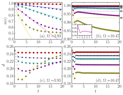
Figure 1: Momentum occupation $n(\epsilon_{{\bm{k}}})$ for energy $\epsilon_{{\bm{k}}}=-0.4$ (upper panels) and double occupation (lower panels) at stroboscopic times $2\pi m/\Omega$ for $U=0.1,0.3,0.5,0.8,1.2$ from top to bottom curves in each panel. Panels (a) and (c): $\Omega=3.93$, panels (b) and (d): $\Omega=10.47$. Symbols with dashed lines: DMFT data, continuous lines: perturbative predictions from Eqs. (20) and (31). Inset of panel (b): same as main panel for $U=0.8$, but showing complete time evolution (i.e. also non stroboscopic times). The arrows in panel (b) show the predictions of Eq. (II.3).

In Fig. 1 we show the single-particle occupation $n(\epsilon_{{\bm{k}}})$ at stroboscopic times for a specific value of $\epsilon$ for $\Omega=3.93$ and $\Omega=10.47$, which lie in the Fermi golden-rule regime and in the prethermalization regime, respectively. We find that the perturbative predictions from Eqs. (20) and (31) capture well the initial slope of the occupation in the linear absorption regime, as well as the prethermalization plateau predicted by Eq. (II.3) for $\Omega=10.47$. For later times the numerical results approach the infinite-temperature value $n_{\beta\to 0}(\epsilon)$ $=$ $0.5$. As expected, the agreement between the DMFT results and the perturbative predictions improves with decreasing $U$, where the prethermalization plateau extends to longer times. In the inset of Fig. 1 we show the time evolution of the occupation $n(\epsilon)$ at $U=0.8$. At $t\sim 2$-$4$ the quasi-periodic prethermalization regime begins where $n(\epsilon)$ is constant at stroboscopic times. The double occupation (lower panels of Fig. 1) also shows a prethermalization plateau at high frequency, while it evolves towards its infinite temperature value for $\Omega$ in the Fermi golden-rule regime.

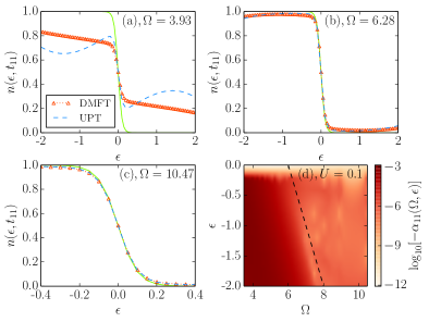
Figure 2: (a), (b), (c): single particle occupations for a driving term with $U=0.5$, computed with DMFT (red triangles, with initial inverse temperature $\beta$ $=$ $20$) and from perturbation theory (blue dashed lines, initially in the ground state) at an intermediate time, $t_{11}$ $=$ $11T$, for $\Omega$ $=$ $2\pi/T$ $=$ $3.93$, $6.28$, and $10.47$, respectively; the initial state is prepared with $U$ $=$ $0$. The green continuous line shows the free initial thermal state at $\beta$ $=$ $20$. The UPT prediction in panel (c) negligibly differs from the prethermalization plateau predicted by Eq. (II.3). (d): Excitation over one period, measured as $\alpha_{m}(\epsilon,\Omega)$ (see main text) for $U=0.1$ using DMFT. The black dashed line corresponds to $\epsilon=-\Omega+6$, which together with $\epsilon=-\Omega$ delimits the Fermi-golden-rule regime.

In Fig. 2 we plot $n(\epsilon,t_{m})$ as a function of $\epsilon$ after a given number of periods ($m=11$). Panel (a) corresponds to a frequency such that every value of $\epsilon$ gives rise to linear terms, which are on the contrary absent for $\Omega=10.47$, see panel (c). Panel (b) refers to an intermediate case ($T=1.0$, $\Omega=2\pi$), where only the boundary values of $\epsilon$ (i.e. $\epsilon\gtrsim-2$ and $\epsilon\lesssim 2$) give linear contributions and thus at $t_{m}\gg T$ differ from the DMFT data. Finally, panel (d) shows the absorption of energy, measured by the slope $\alpha_{m}(\epsilon,\Omega)\equiv n(\epsilon,m2\pi/\Omega)-n(\epsilon,(m-1)2\pi/\Omega)$, which becomes small for $\Omega>6-\epsilon$, as predicted by the perturbative calculation (shown with a dashed line for $m$ $=$ $11$). We point out that the regime of validity of the DMFT calculation with iterative perturbation theory does not allow to explore small values of the frequency ($\Omega\lesssim 1$) where the other boundary ($\epsilon=-\Omega$) lies.

VI Conclusions

In conclusion, we discussed the analogue of prethermalization in periodically driven systems. A weakly interacting system can synchronize into a quasi-steady state with nontrivial properties, before reaching the infinite temperature state generic for the long-time behavior of driven non-integrable systems. This stroboscopic prethermalization is a consequence of the existence of a macroscopic set of operators which are almost conserved by the time evolution over one period. Stroboscopic prethermalization thus provides a way to engineer quantum states with a nontrivial effective dynamics, alternative to the a high frequency expansion. These states reflect the properties of perturbative Floquet states, which can be very different in nature from the exact Floquet states.

Appendix A Phase-space argument for the Hubbard model in infinite-dimensions

As discussed in Sec. II.3, the single-particle occupations Eq. (29) at long times (i.e. $t_{m}\gg T$) display two regimes, namely the Fermi-golden rule absorption regime and the stroboscopic prethermalization regime, depending on the value of $\Omega$ and $\epsilon$. Here we discuss these regimes for the specific case of the driven Hubbard interaction by rewriting Eq. (30) and applying a phase-space argument.

As a first step, we express $J_{\epsilon}(\omega)$ in terms of

$$R(s) \equiv\int\limits_{-\infty}^{\infty}d\epsilon\,n(\epsilon)\,\rho(\epsilon)\,e^{is\epsilon}\,,$$ (32)

using a Fourier representation of the delta function:

$$J_{\epsilon}(\omega) =\int\limits_{-\infty}^{\infty}\frac{ds}{2\pi}\left[n(\epsilon)e^{i(\epsilon+\omega)s}-\bar{n}(\epsilon)e^{-i(\epsilon+\omega)s}\right]R(s)^{3}\,.$$ (33)

We also note that for an initial zero-temperature state (with $n(\epsilon)$ $=$ $\Theta(-\epsilon)$), $J_{\epsilon}(\omega)$ is zero unless $|\epsilon|$ $\leq$ $|\omega|$ $\leq$ $3D+|\epsilon|$, where $D$ is the half-bandwidth.

A partial fraction decomposition of the functions in Eq. (30) and a shift of the integration variable yield

$$F_{n,p}(\epsilon,t_{m}) =\frac{F^{(1)}(\epsilon,t_{m},n\Omega)-F^{(1)}(\epsilon,t_{m},p\Omega)}{(n-p)\Omega}\,,~{}(n\neq p)$$

$$F_{n,n}(\epsilon,t_{m}) =F^{(2)}(\epsilon,t_{m},n\Omega)\,,$$ (34)

where we defined

$$F^{(N)}(\epsilon,t_{m},E) \equiv\int\limits_{-\infty}^{\infty}d\omega\,\frac{\sin^{2}(\omega t_{m}/2)}{\omega^{N}}J_{\epsilon}(\omega+E)\,.$$ (35)

Consider first the case of zero (or sufficiently low) temperature of the initial state and $|\epsilon|$ $\leq$ $|\Omega|$ $\leq$ $3D+|\epsilon|$. Then a term linear in $t_{m}$ contributes to $F(\epsilon,t_{m})$, namely ($E$ $=$ $|n\Omega|$, $N$ $=$ 1,2, $x$ $=$ $(\omega-E)t_{m}$)

$$F^{(N)}(\epsilon,t_{m},E) =t_{m}^{N-1}\int\limits_{-\infty}^{\infty}dx\,\frac{\sin^{2}(x/2)}{x^{N}}J_{\epsilon}(\tfrac{x}{t_{m}}+E)$$

$$\sim\delta_{N2}\frac{\pi t_{m}}{2}J_{\epsilon}(E)\,~{}~{}(t_{m}\to\infty)$$ (36)

This corresponds to the Fermi golden rule regime with a linear-in-time growth of $n(\epsilon,t_{m})$. On the other hand, if $\Omega$ is outside the indicated interval, the denominators are never zero (for zero temperature) and a stroboscopic prethermalization plateau is attained.

In all cases we can rewrite the integrals more compactly by using the identities

$$\frac{\sin^{2}(\omega t/2)}{\omega} =\frac{1}{2}\int\limits_{0}^{t}du\,\sin(\omega u)\,,$$ (37)

$$\int\limits_{0}^{\infty}d\omega\,\frac{\sin^{2}(\omega t/2)}{\omega^{2}}\cos(\omega s) =\frac{\pi}{4}(t-s)\Theta(t-s)\,,$$ (38)

and taking the symmetries of the $\omega$ and $s$ integrals into account. We obtain

$$F^{(1)}(\epsilon,t_{m},E) =-\frac{1}{2}\int\limits_{0}^{t_{m}}ds\,\text{Im}\bigg{[}R(s)^{3}\;\times$$ (39)

$$~{}~{}~{}~{}~{}~{}\Big{(}n(\epsilon)e^{i(\epsilon+E)s}+\bar{n}(\epsilon)e^{-i(\epsilon+E)s}\Big{)}\bigg{]},$$

$$F^{(2)}(\epsilon,t_{m},E) =\frac{1}{2}\int\limits_{0}^{t_{m}}ds\,\text{Re}\bigg{[}R(s)^{3}\;\times$$ (40)

$$~{}~{}~{}~{}~{}~{}\Big{(}n(\epsilon)e^{i(\epsilon+E)s}-\bar{n}(\epsilon)e^{-i(\epsilon+E)s}\Big{)}\bigg{]}.$$

These expressions are suitable for numerical evaluation; they can be further simplified for the zero-temperature case.

References

- Shirley (1965) J. H. Shirley, Phys. Rev. 138, B979 (1965).
- Sambe (1973) H. Sambe, Phys. Rev. A 7, 2203 (1973).
- Breuer, H.P., Dietz, K., and Holthaus, M. (1990) Breuer, H.P., Dietz, K., and Holthaus, M., J. Phys. France 51, 709 (1990).
- Grifoni and Hänggi (1998) M. Grifoni and P. Hänggi, Phys. Rep. 304, 229 (1998).
- Oka and Aoki (2009) T. Oka and H. Aoki, Phys. Rev. B 79, 081406 (2009).
- Kitagawa et al. (2011) T. Kitagawa, T. Oka, A. Brataas, L. Fu, and E. Demler, Phys. Rev. B 84, 235108 (2011).
- Iadecola et al. (2013) T. Iadecola, D. Campbell, C. Chamon, C.-Y. Hou, R. Jackiw, S.-Y. Pi, and S. V. Kusminskiy, Phys. Rev. Lett. 110, 176603 (2013).
- Kitagawa et al. (2010) T. Kitagawa, E. Berg, M. Rudner, and E. Demler, Phys. Rev. B 82, 235114 (2010).
- Lindner, Refael, and Galitski (2011) N. Lindner, G. Refael, and V. Galitski, Nature Physics 7, 490 (2011).
- Wang et al. (2013) Y. H. Wang, H. Steinberg, P. Jarillo-Herrero, and N. Gedik, Science 342, 453 (2013).
- Fausti et al. (2011) D. Fausti, R. I. Tobey, N. Dean, S. Kaiser, A. Dienst, M. C. Hoffmann, S. Pyon, T. Takayama, H. Takagi, and A. Cavalleri, Science 331, 189 (2011).
- Hu et al. (2014) W. Hu, S. Kaiser, D. Nicoletti, C. R. Hunt, I. Gierz, M. C. Hoffmann, M. Le Tacon, T. Loew, B. Keimer, and A. Cavalleri, Nat. Mater. 13, 705 (2014).
- Goldman and Dalibard (2014) N. Goldman and J. Dalibard, Phys. Rev. X 4, 031027 (2014).
- Mentink, Balzer, and Eckstein (2015) J. H. Mentink, K. Balzer, and M. Eckstein, Nat. Commun. 6, 6708 (2015).
- (15) R. V. Mikhaylovskiy, E. Hendry, A. Secchi, J. H. Mentink, M. Eckstein, A. Wu, R. V. Pisarev, V. V. Kruglyak, M. I. Katsnelson, T. Rasing, and A. V. Kimel, arXiv:1412.7094 .
- (16) A. P. Itin and M. I. Katsnelson, arXiv:1401.0402 .
- Först et al. (2011) M. Först, C. Manzoni, S. Kaiser, Y. Tomioka, Y. Tokura, R. Merlin, and A. Cavalleri, Nature Physics 7, 854 (2011).
- Polkovnikov et al. (2011) A. Polkovnikov, K. Sengupta, A. Silva, and M. Vengalattore, Rev. Mod. Phys. 83, 863 (2011).
- Kinoshita, Wenger, and Weiss (2006) T. Kinoshita, T. Wenger, and D. S. Weiss, Nature 440, 900 (2006).
- Trotzky et al. (2012) S. Trotzky, Y.-a. Chen, A. Flesch, I. P. McCulloch, U. Schollwöck, J. Eisert, and I. Bloch, Nature Physics 8, 325 (2012).
- Altshuler et al. (1997) B. L. Altshuler, Y. Gefen, A. Kamenev, and L. S. Levitov, Phys. Rev. Lett. 78, 2803 (1997).
- Gornyi, Mirlin, and Polyakov (2005) I. V. Gornyi, A. D. Mirlin, and D. G. Polyakov, Phys. Rev. Lett. 95, 206603 (2005).
- Basko, Aleiner, and Altshuler (2006) D. Basko, I. Aleiner, and B. Altshuler, Annals of Physics 321, 1126 (2006).
- Rigol et al. (2007) M. Rigol, V. Dunjko, V. Yurovsky, and M. Olshanii, Phys. Rev. Lett. 98, 050405 (2007).
- Langen et al. (2015) T. Langen, S. Erne, R. Geiger, B. Rauer, T. Schweigler, M. Kuhnert, W. Rohringer, I. E. Mazets, T. Gasenzer, and J. Schmiedmayer, Science 348, 207 (2015).
- Kollar, Wolf, and Eckstein (2011) M. Kollar, F. A. Wolf, and M. Eckstein, Phys. Rev. B 84, 054304 (2011).
- Berges, Borsányi, and Wetterich (2004) J. Berges, S. Borsányi, and C. Wetterich, Phys. Rev. Lett. 93, 142002 (2004).
- Moeckel and Kehrein (2008) M. Moeckel and S. Kehrein, Phys. Rev. Lett. 100, 175702 (2008).
- Gring et al. (2012) M. Gring, M. Kuhnert, T. Langen, T. Kitagawa, B. Rauer, M. Schreitl, I. Mazets, D. A. Smith, E. Demler, and J. Schmiedmayer, Science 337, 1318 (2012).
- Russomanno, Silva, and Santoro (2012) A. Russomanno, A. Silva, and G. E. Santoro, Phys. Rev. Lett. 109, 257201 (2012).
- Lazarides, Das, and Moessner (2014a) A. Lazarides, A. Das, and R. Moessner, Phys. Rev. Lett. 112, 150401 (2014a).
- Lazarides, Das, and Moessner (2015) A. Lazarides, A. Das, and R. Moessner, Phys. Rev. Lett. 115, 030402 (2015).
- Abanin, De Roeck, and Huveneers (2014) D. Abanin, W. De Roeck, and F. Huveneers, ArXiv e-prints (2014), arXiv:1412.4752 [cond-mat.dis-nn] .
- D’Alessio and Polkovnikov (2013) L. D’Alessio and A. Polkovnikov, Annals of Physics 333, 19 (2013).
- Ponte et al. (2015a) P. Ponte, A. Chandran, Z. Papić, and D. A. Abanin, Annals of Physics 353, 196 (2015a).
- Ponte et al. (2015b) P. Ponte, Z. Papić, F. Huveneers, and D. A. Abanin, Phys. Rev. Lett. 114, 140401 (2015b).
- Roy and Das (2015) A. Roy and A. Das, Phys. Rev. B 91, 121106 (2015).
- Lazarides, Das, and Moessner (2014b) A. Lazarides, A. Das, and R. Moessner, Phys. Rev. E 90, 012110 (2014b).
- D’Alessio and Rigol (2014) L. D’Alessio and M. Rigol, Phys. Rev. X 4, 041048 (2014).
- (40) A. Eckardt and E. Anisimovas, arXiv:1502.06477 .
- Dittrich et al. (1998) T. Dittrich, P. Hänggi, G. L. Ingold, B. Kramer, G. Schön, and W. Zwerger, Quantum Transport and Dissipation (Wiley-VCH, Weinheim, 1998).
- Note (1) Unitary transformations of the periodic Hamiltonian are also used in Ref. \rev@citealpAbanin_pp14, but in that case with the aim of finding a many-body localized cycle Hamiltonian , i.e. a Hamiltonian with a set of true integrals of motion.
- Note (2) The statistical enesemble is the periodic Gibbs ensemble of Ref. \rev@citealpLazarides_PRL14 evaluated at stroboscopic times.
- Aoki et al. (2014) H. Aoki, N. Tsuji, M. Eckstein, M. Kollar, T. Oka, and P. Werner, Rev. Mod. Phys. 86, 779 (2014).
- Eckstein, Kollar, and Werner (2010) M. Eckstein, M. Kollar, and P. Werner, Phys. Rev. B 81, 115131 (2010).
- Tsuji and Werner (2013) N. Tsuji and P. Werner, Phys. Rev. B 88, 165115 (2013).