Nonlocal and quasi-local field theories
E. T. Tomboulis111e-mail: tomboulis@physics.ucla.edu
Department of Physics and Astronomy, UCLA, Los Angeles, CA 90095-1547
Abstract
We investigate nonlocal field theories, a subject that has attracted some renewed interest in connection with nonlocal gravity models. We study, in particular, scalar theories of interacting delocalized fields, the delocalization being specified by nonlocal integral kernels. We distinguish between strictly nonlocal and quasi-local (compact support) kernels and impose conditions on them to insure UV finiteness and unitarity of amplitudes. We study the classical initial value problem for the partial integro-differential equations of motion in detail. We give rigorous proofs of the existence but accompanying loss of uniqueness of solutions due to the presence of future, as well as past, “delays”, a manifestation of acausality. In the quantum theory we derive a generalization of the Bogoliubov causality condition equation for amplitudes, which explicitly exhibits the corrections due to nonlocality. One finds that, remarkably, for quasi-local kernels all acausal effects are confined within the compact support regions. We briefly discuss the extension to other types of fields and prospects of such theories.
1 Introduction
Nonlocal field theories is a subject with long, albeit spotty, history. Despite the success of perturbative renormalization in QED in the late forties, the idea that local interactions may be a low energy approximation to fundamental underlying nonlocality of interactions continued to be prominent in the fifties and the subject of many investigations [1]. Subsequently, nonlocality was considered mostly in the context of axiomatic field theory [2]. In more recent years it has attracted renewed interest in connection with nonlocal theories of gravity [3] - [9], as well as the nonlocality of string field theory vertices and various nonlocal models in cosmology and other areas, see [10] and extensive reference list therein.
Despite this past work, basic issues have been left in a murky state. It has long been realized, more or less explicitly, that UV finiteness (or at least superrenormalizability in the presence of gauge interactions) can be achieved by nonlocal interactions. At the same time, unitarity can be preserved, at least perturbatively, provided appropriate analyticity conditions can be imposed on the nonlocal interactions. Causality, however, is a central concern whose investigation has remained woefully inadequate, both in the classical theory, where it is inexorably connected with the mathematically proper formulation of the initial value problem (IVP), and in the quantum theory.
In this paper we address some of these issues in a more systematic way in the simplest field theory context, i.e. scalar field theories. (We comment on the extension to other theories in the last section.) To set the stage we recall that often, both in the older and more recent literature, nonlocal interactions have been introduced through the insertion of an operator of the general form
| (1.1) |
where, in many instances, is an entire analytic function. Note that is then itself an entire function possessing no zeroes anywhere in the complex plane. In many cases is simply a polynomial. For example, gives a generic form of vertices in string field theory, i.e., vertices of the form for, say, the dilaton field . For Euclidean signature this has the explicit integral kernel form
| (1.2) |
For Minkowski signature, though, the operator on the l.h.s. of (1.2) is ill-defined (except, of course, at ). This is the reason why only even power polynomials for were considered in the older non-local QFT literature,222In the fifties (1.3) was referred to as the “decay” choice as opposed to the “oscillatory” choice involving rational functions. e.g.,
| (1.3) |
where
| (1.4) |
This ensures well-defined kernels on the whole real axis . In the more recent literature more elaborate choices of well-defined kernels employing transcendental entire functions have been considered [3], [6].
For our purposes, there are three features of the nonlocal interactions introduced via (1.1) that are of interest. First, is such that the Fourier transform kernel is an entire analytic function of . This is connected to unitarity in amplitudes. The second feature is that the resulting interactions, even though they may exhibit rapid or exponential fall-off, are truly non-local: any two spacetime points and are connected by the interaction integral kernels . This should generally imply some acausal behavior.
Finally, since entire functions possess convergent series expansions333One should keep in mind, however, that any truncation of such an expansion, at any order, will fail to reproduce all the remarkable properties of transcendental entire functions, such as, for example, those embodied in Piccard’s theorems. about any point, (1.1) may be viewed as representing “infinite order” derivative interactions. Attempts have been made historically to deal with such interactions in some sort of Hamiltonian formalism with infinite order derivatives. This has apparently been the source of a great deal of confusion in the literature. Typical of more recent work is the scheme in [11] for -dimensional, i.e., mechanics systems in which an infinite order Lagrangian is truncated to order as a member of a hierarchy . In cases where all higher derivatives appear only in the interaction terms, this allows “reduction” of the IVP to that of a second order system. It singles out a subset of solutions that encompass perturbation theory. This scheme was employed also in [12] in the investigation of the problems associated with the nonlocality of string field theory vertices (cf. (1.2)). As pointed out in [12], however, such schemes completely obscure the existence of the (infinite) class of all other solutions exhibiting the very features one might expect associated with the nonlocal nature of the vertices such as lack of uniqueness of the IVP. As a general remark in this connection, finite order higher (time) derivative interactions can indeed be cast into the Hamiltonian formalism by the so-called Ostrogradsky construction. In mathematical terms this construction amounts to the usual procedure of rewriting a -th order ordinary differential equation (ODE) as a system of coupled first-order ODEs. One cannot, though, view a transcendental differential operator (pseudo- or fractional-differential operator) as, e.g., (1.1), as the “limit” of this procedure.
In this paper we consider a wide class of nonlocal theories, which includes many of the form (1.1) as a special subclass. Nonlocal interactions in this wide class are always defined by specifying the appropriate integral kernel. This includes the cases where a kernel may be associated with a transcendental differential operator (cf. (1.3) - (1.4) above). Definition by the appropriate integral kernel allows a consistent, mathematically well-defined formulation in all cases. By the same token we eschew any series expansions in derivatives, always dealing with the complete nonlocal kernel . As implied by the preceding remarks, such expansions are generally a bad idea. They derail a proper posing of the classical IVP by replacing the integro-differential equations of motion by truncated higher derivative differential equations. In the quantum theory, e.g., for various models in [3] - [10], unitarity can appear to be grossly violated in inappropriate truncations at any finite order by the presence of increasingly large numbers of ghosts, which, however, are not there in the untruncated theory where the correct analyticity properties are regained. In fact, as we will see, kernels that do not even possess expansions about every point in -space may comprise the physically most promising class of nonlocal interactions.
An outline of the paper is as follows. In the following section 2 we introduce interactions of delocalized fields. We then impose conditions on the allowed interactions. Specifically, we give, a precise statement of the conditions imposed on the Fourier transform of allowed kernels dictated by the requirements of good UV behavior and unitarity. Among kernels that may accommodate these requirements we distinguish between strictly nonlocal and quasi-local (bounded support) kernels.
In section 3 we make a detailed study of the classical IVP using modern fixed-point (contraction) techniques. We first review the case of local interactions where the equations of motion are partial differential equations (PDE) giving a proof of existence and uniqueness of solutions. We then turn to the case of nonlocal interactions specified by a given integral kernel. Varying the action now gives equations of motion that are non-linear partial integro-differential equations. This makes the contrast to the local case rather transparent. Because of the “spilling-over” effect of the nonlocal kernel one now has an IVP problem with both past and future “delays”. Differential and integro-differential/functional equations with past delays have been extensively studied in recent decades in a vast literature.444This is because “real-world” modeling of many systems in physics, engineering, biology, economics and other fields very often must include dependence on past history (memory). See, e.g., [14]. They imply specification of functions as data over a time interval (as opposed to just data on an initial time hypersurface). In our case some specification must also be made in the future delay region. We then prove (local) existence of solutions but uniqueness is totally lost. Physics, however, is more than mathematics. If the delay regions are of strictly finite extent of length order , they will be masked by the uncertainties in any measurements probing physics at scales larger than . This situation arises with quasi-local interactions. A proper formulation of such considerations, however, can only be given in the full quantum context (section 5). In a similar vein, if one assumes quasi-local interactions being asymptotically turned off (free fields in asymptotic regions) and such that a global existence result can be established, uniqueness is recovered as shown at the end of section 3.555Similar existence results in the case of the string field theory inspired kernel (1.1) in (where it is well defined) with a “future” asymptotic boundary condition were obtained in [13].
In section 4 we digress to briefly consider a Hamiltonian formulation. The standard procedure gives a positive “Hamiltonian”. Due to the nonlocal interactions, however, it necessarily contains implicit functional dependence on a range of times and thus fails to reproduce the correct equations of motion. The standard Hamiltonian procedure is simply inapplicable in the case of general nonlocal interactions. In the case of quasi-local (compact support) interactions, however, the results on the IVP in the previous section suggest that one should instead define a smeared Hamiltonian appropriate to time-blocking over intervals longer than scale . This procedure then indeed correctly reproduces the equations of motion for evolution over such time blocks.
In section 5 we finally turn to the quantum theory. Quantization is straightforwardly performed via the path integral. The rapid decay properties required of allowed kernels, as given in section 2, ensure that any graph is UV finite for wide classes of scalar potentials. Similarly their analyticity properties, chosen so as not to modify the Cutkosky cutting rules, ensure that, at least graph by graph, unitarity is preserved. The main concern, however, is causality. We examine the structure of the effective propagator that results from incorporating the nonlocal kernels it joins to at vertices. This allows us to obtain a generalization of the Bogoliubov causality condition equation in the presence of nonlocal interactions. This generalized equation shows how the Bogoliubov condition for local interactions gets modified by nonlocality. Remarkably, for interaction kernels of compact support of size , it implies that all non causal effects remain confined within scale .
Some further discussion of these results and their extension and application to other theories is given in the concluding section 6. The reader who is not interested in the details of the classical IVP can go directly from section 2 to section 5. We work mostly in spacetime dimension but most considerations extend to general straightforwardly. We use standard physics and mathematical notations; in particular, denotes the space of continuous functions on domain , and denotes the norm: .
2 Delocalized field interactions
We consider the simplest case of a real scalar field, the extension to complex or multi-component scalar fields being immediate. The Lagrangian with local non-derivative interactions is then given by
| (2.1) |
with . General polynomial interactions are allowed in , though it suffices keep in mind the standard example. Non-polynomial interactions, in particular interactions ensuring Lipschitz-continuity of , e.g., , are also of interest, as we will see, in connection with the classical IVP.
The class of non-local versions of (2.1) considered in this paper is obtained by replacing the field in by a delocalized field , i.e.
| (2.2) |
The delocalized field is defined by
| (2.3) |
in terms of a delocalization kernel . The local action (2.1) is then obtained as the special case . The kernel is a scalar density function defined on the spacetime manifold , i.e., if is specified in one frame, under it is given by . (We only need consider here so we ignore the distinction between scalars and scalar densities.)
The kernel and its Fourier transform , introduced through
| (2.4) |
will be the quantities of main concern below.
It should be noted that in any interaction term in , such as , the delocalized fields interact at a common spacetime point , resulting in an interaction . This ensures that each interaction vertex is proportional to a single spatial momentum conservation delta-function (times an energy conservation delta-function) which, as it is well-known, is a sufficient condition for cluster decomposition. This would not necessarily be the case for generic nonlocal interactions
| (2.5) |
Feynman rules for diagrammatic expansion can, of course, be read off the non-local Lagrangians (2.2) - (2.3), or (2.5), [15] just as in the local case (2.1).
In what follows we adopt a general point of view and consider a wide class of delocalization integral kernels. Kernels in this wide class cannot necessarily be represented by an expansion in derivatives about every point, those associated with operators of the form (1.1) being a particular subclass of possible non-local interactions. In general, the choice of the kernel in (2.3) is restricted by the imposition of physical requirements. The first two requirements are controllable UV behavior and unitarity, at least within the perturbative expansion. These conditions constrain . Causality and other considerations may then further guide the choice of in particular theories.
The two fundamental properties we require to satisfy are:
-
(I)
is an element of the space of functions of rapid decay, commonly denoted by .
A function is: (i) infinitely differentiable; (ii)
(2.6) for every pair of nonnegative integer multi-indices , with the notation and . Note that the boundedness of shows that
(2.7) i.e., a function of rapid decay and all its derivatives in fact vanish faster than any negative power of its arguments as .
-
(II)
is an entire analytic function, i.e. it is analytic in each component in the entire complex -plane.
Condition (I) is dictated by the requirement of good UV behavior, and condition (II) by that of unitarity.
We now define two classes of vertices constructed from products of delocalized fields (2.3) with kernels that can accommodate the conditions (I), (II) above:
-
(a)
Quasi-local interaction vertices with integral kernels which are elements of the space of functions of bounded support, commonly denoted by .
A function : (i) is infinitely differentiable; (ii) vanishes identically outside a compact (bounded, closed) set, i.e. has bounded support (the closure of the set on which the function has non-zero value).
-
(b)
Strictly nonlocal interaction vertices with integral kernels which are elements of but not of , i.e. elements of the space of functions of rapid decay that do not have compact support.
An example of a nonlocal kernel, characterized by a length scale , would be . Quasi-local kernels are naturally obtained by standard smoothing (‘mollifying’) of over a length scale . In other words, they may be taken as elements of a delta-family, the local limit being recovered when . It is important to note here that a quasi-local kernel of such or similar shape of size will have a Fourier transform which is essentially flat for real momenta less than of order , and rapidly decaying for momenta above ; in the local limit one recovers constant for all . A nonlocal kernel will have a Fourier transform of approximately similar behavior if the kernel decays sufficiently fast outside a sufficiently small region of size . It should also be noted that there are points about which quasi-local kernels, though functions, have Taylor expansions of zero radius of convergence.
We now recall some mathematical facts (see, e.g., [16]). supplemented with an appropriate notion of convergence becomes , the test function space of distributions, the latter being defined as elements of , the dual space to . supplemented with an appropriate notion of convergence becomes , the test function space of tempered distributions which are elements of the dual space . Thus our delocalized fields replace local fields (tempered distributions in the usual formalism) by their convolution with an element of the corresponding test function (sub)space.
A basic result for us here is that if a function is in its Fourier transform exists and is also in . Now, is a subspace of the space of functions of rapid decay . Note, however, that the Fourier transform of a function in will not be also in , though, of course, it will in . (This is in fact what necessitates the introduction of in order to have the distributional extension of classical Fourier theory.) It follows that the Fourier transforms of kernels of both types (a) and (b) above satisfy condition (I).
Another basic fact is that the Fourier transform of a function in is an entire analytic function of its argument. Thus, the Fourier transforms of functions in form a subset of consisting of functions that can be extended from the real axis to the complex domain as entire functions.666Given appropriate norms, these functions comprise the sequence of spaces of entire functions in the Gel’fand-Shilov extension of generalized function theory into the complex plane [16]. They possess special properties of potential interest in particular models of interactions, but we will not make specific use of them in the general considerations in this paper. It follows that the Fourier transforms of quasi-local kernels (a) above satisfy also condition (II). In contrast, condition (II) is not automatically satisfied for general non-local kernels (b), i.e. general elements of , though it can be satisfied for large subclasses of them, (1.4) being a simple example.
Within this framework, operators of the form (1.1) are considered as defined in terms of the corresponding integral kernels, as exemplified by the r.h.s. in (1.2), (1.3). Thus, (1.4), being indeed of rapid decay, gives a non-local interaction of type (b) above. Note also that it may not always be possible to give a closed kernel form in both coordinate and -space, but being in in either space is sufficient. In contrast, in the case of (1.2) for the integral kernel is not of rapid decay for large negative values of its argument , and is not included in the class (b); its Fourier transform cannot be properly defined to satisfy (II) with the consequent lack of analyticity presumably implying instability.
In general, assuming they are well-defined by appropriate choice of the function , from among the kernels that may be introduced via (1.1) a large subset are of the non-local type (b). Another subset though, e.g., some of those employed in [3], also [6], though well-defined, are not of rapid decay and do not belong to the class (b). On the other hand, general kernels of type (b) constitute a rather larger set than the rapid decay subset that can be generated via (1.1). Quasi-local vertices of type (a) cannot, of course, be generated via (1.1).
In summary, we introduced non-locality by the replacement of fields in local interaction vertices by delocalized fields, i.e., replacement of (2.1) by (2.2) - (2.3). The Fourier transform of the delocalization kernel is required to satisfy the fundamental conditions (I) and (II) above. We then defined two general classes of kernels, the non-local kernels of rapid decay, and the quasi-local kernels of bounded support. Both satisfy condition (I). Quasi-local kernels also satisfy condition (II). General non-local kernels do not automatically satisfy condition (II), but a large subset in this class does. In what follows we examine the extent to which these classes of interactions may allow physically viable theories.
3 The classical theory - time evolution and IVP
The equation of motion is derived as usual by varying the action (2.2). The resulting field equation is
| (3.1) |
with, as usual, . (3.1) is a nonlinear wave functional equation in spacetime dimensions. The functional field dependence introduces “delays”. Differential/functional equations with past delays have been extensively studied in recent years. The novel feature here is that the delocalized field interactions introduces future, as well as past, delays. We need then examine what effect this has on time evolution and the existence of solutions of (3.1). In this section we set since this simplifies formulas without affecting the main issues we discuss here - the non-zero mass case is quite analogous.777In any case, one may always include the mass term as a local addition to the potential as is usually done in the mathematical literature.
A common approach to existence and uniqueness questions for nonlinear wave equations is to convert them to an integral equation. This is done by substituting the non-linear interaction for the inhomogeneous term in the known solutions to the linear inhomogeneous problem. In the case of (3.1) with in () d’Alembert’s formula results in the integral equation
| (3.2) | |||||
whereas in () Kirchhoff’s formula leads to
| (3.3) |
In (3.2) and (3.3) denotes the solution, in and , respectively, to the linear homogeneous problem
| (3.4) |
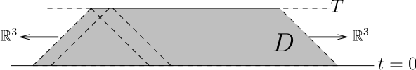
In (3.2) denotes the triangular region (domain of dependence) enclosed by the axis and the two characteristics lines emanating from the point . In (3.3) the closed ball in centered at and of radius .888Note the amusing fact that whereas is -dimensional, is only -dimensional. This is because Huygen’s principle holds in odd space dimensions but not for - the latter behaving like even space dimensions. The presence of the unrestricted -integration in (3.2) and (3.3) is due to the nonlocal nature of the kernel , and is the crucial feature distinguishing the nonlocal from the local case.
The integral equation formulation allows application of fixed point theorems to investigate existence of solutions [17]. In an appropriately defined space of functions (cf. below) the r.h.s. of (3.2) or (3.3) defines a nonlinear mapping . A fixed point of this mapping, i.e.
| (3.5) |
if it exists, is then a solution to these integral equations. This formulation also makes immediately apparent the difference between the local and nonlocal cases.
3.1 Local interaction
It will be useful to first review here an existence and uniqueness proof of this kind [17] in the familiar case of local interactions, i.e. (3.3) with . The r.h.s. of (3.3) then defines the mapping:
| (3.6) |
with . The solution to the linear problem (3.4) satisfies initial data
| (3.7) |
Let denote the set of functions
a subset of the complete metric space . Assuming smooth in (3.7), is smooth, and it follows that if there exists a constant such that
| (3.8) |
For the mapping (3.6) then, if one has
| (3.9) | |||||
The constant comes from
| (3.10) | |||||
where it is assumed that is at least twice continuously differentiable and use is made of (3.8), and also . Take small enough and/or couplings in weak enough so that . It follows then from (3.9) that the mapping is a contraction. Similarly, if ,
| (3.11) | |||||
so that indeed, under the same conditions, .
Starting then with some initial field configuration , one obtains a succession of configurations by
| (3.12) |
By the contraction mapping theorem this has a unique fixed point which provides the unique solution to (3.5) - (3.6) on (Fig 1). Further arguments [17], in particular consideration of the corresponding integral equations for derivatives, show that, assuming is smooth, all derivatives are similarly bounded, so the solution is in fact smooth. Depending on the form of the interaction continuation of the solution to any , i.e. global existence, may be proven in many cases (such as a interaction). In fact, under the stronger assumption that the interaction is Lipschitz continuous it may be proven that a weak solution always exists for any .
3.2 Nonlocal interaction
In the nonlocal case is given by the r.h.s. of (3.3) involving nonlocal kernel :
| (3.13) |
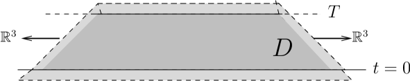
In considering (3.12) the difference from the local case is now apparent. It is no longer true that to compute one needs only in . There is a “spill-over” or “delay” effect since in (3.3) is connected to which now can range outside . Similarly, in the case, on the r.h.s. in (3.2) the point is connected via the kernel to which can range outside . Note that there is a past as well as a future delay. The delay regions then form a collar in (Fig. 2). For kernels of bounded support this collar is of finite extent. For nonlocal kernels this extent is strictly infinite even though, for sufficiently rapid decay rate, it may appear essentially finite for all practical purposes.
3.2.1 Quasi-local interactions
We now restrict to the case of bounded support kernels of scale . Let be the extension of the domain to include a collar region of width with integer . Given some initial configuration , to compute in via the mapping one needs in ; to compute in one needs in , hence in , and so on: for , to compute in one needs in . Since, to apply a fixed point argument, one sees that the field need be computed at essentially all points. This may at first sight appear not to be a problem since, given some initial configuration , say, identically vanishing except inside some bounded spacetime region, one may apply the mapping to generate the field value of subsequent configurations at any spacetime point. Because involves integration, however, it is easily seen that upon subsequent iterations it will generate fields that grow as at spacetime point . This was already seen in the local interaction case above; there, however, for solutions on a fixed interval only the values of fields within this interval were needed in successive iterations. In contrast, in the case of nonlocal interaction to establish existence of solutions on in the same manner would require field values at all points with the attendant boundedness problem. We must then proceed differently.
The existence of local solutions on suitably small intervals can, in fact, be demonstrated in the case of nonlocal interaction, but uniqueness is completely lost. To demonstrate existence on one has to extend the definition of the mapping to specify fields in the collar region . In the past delay region of the collar, , the fields are specified as initial data (cf. [14]). One may take999Alternatively, one may specify an arbitrary smooth function on as past delay initial data, and replace (3.14) with and . the solution of the linear problem (3.4) with initial data
| (3.14) |
at some time where , and set on . Let
| (3.15) |
is specified by extending the values , given by into the collar region in some prescribed continuous fashion. E.g., parametrizing points in by
| (3.16) |
where denotes the outward (timelike) normal at , we may define
| (3.17) |
In (3.17) is a function such that and in a neighborhood of . Adopting one such prescription, (3.15) defines then a mapping on .
Let denote the set of functions
Assuming smooth in (3.14), it follows that if there exists a constant such that
| (3.18) |
Furthermore,
| (3.19) |
where .
If one has
| (3.20) | |||||
Note also that . Making then use of (3.18), (3.19) and (3.20),
| (3.21) | |||||
Also, for ,
| (3.22) |
Thus, for in ,
| (3.23) |
Similarly, one verifies that
| (3.24) |
Hence, for and/or couplings in the interaction chosen sufficiently small, and is a contraction. It follows that there is a solution to the integral equation (3.3) on satisfying the initial data on .
The solution is unique for a given mapping , but this mapping depends on its specification in the future collar region . There is then a unique solution on for each such choice of specification. In other words, there is local existence but complete loss of uniqueness for the solution of the IVP associated with (3.3) (or (3.2)). This reflects the loss of causality due to the nonlocality of the interaction. To obtain a solution on , in addition to initial data on some past delay region , some specification of fields in the future delay region has to be provided, thus converting the IVP to a combined IVP-BVP of sorts.
For physics at length scales appreciably longer than , however, this dependence on the acausal delay from would be masked in field measurements necessarily averaged over scales longer than order . This becomes even more pertinent when going from the classical to the quantum context where all fluctuations are included (section 5). This suggests that one should consider time evolution smeared over regions of order . We return to this below.
There are circumstances in which uniqueness of the classical IVP can be obtained. This is the case when the nonlocal interactions are confined within the interval for which existence can be demonstrated. This is of particular importance if existence for any , i.e. global existence (at least of a weak solution) can be proven. One may then consider the asymptotic “switching-off of interactions” outside a (large) spacetime region, as commonly done in scattering theory. This is implemented by letting where is a function such that for and for . In the rest of this section we redefine to include the variable coupling .
To obtain a global existence result we will assume that is Lipschitz-continuous, i.e.,
| (3.25) |
for some constant . We also introduce the norm (cf., e.g., [14], [18])
| (3.26) |
Let denote the set of functions
If , one now has
| (3.27) | |||||
using (3.25) and the fact that, in the next to last inequality, due to the bounded support of . For (3.3), with initial data (3.14), we define the mapping by
| (3.28) |
Then
using (3.27) and, again, that due to the compact support of . Since we finally obtain
| (3.29) | |||||
(3.29) holds for any . Take, say, , and the scale and/or couplings in sufficiently small, so that . Then (3.29) shows that is a contraction. It follows that a unique solution to the integral equation (3.3) satisfying the initial data on exists on any interval with .
3.2.2 Stricly nonlocal interactions
The case of strictly nonlocal interactions differs in basic ways. For such interactions the future delay is of infinite extent and each point inside a given domain (Fig. 2) contributes to it. Hence, asymptotic switching off of interactions no longer makes the argument leading to (3.29) possible. The demonstration of local existence of solutions still formally goes through since one may always specify an extension of the mapping over the infinite extent delay region. Existence of an infinity of solutions can thus be established. The causal effects, however, are no longer confined in a (small) finite region and cannot, in principle, be masked at larger scales as in the quasi-local case. Still, strictly nonlocal interactions may approximately behave as quasi-local ones if their delocalization kernel falls off sufficiently rapidly beyond a characteristic scale , the long-range causal tails leaking out at long distances producing extremely small effects.
The classical IVP, though it serves well to demonstrate how nonlocality entails causality problems, is ultimately not of prime physical relevance. For this we have to turn to the quantum theory where one sums over configurations not restricted to solutions of the classical equations of motion.
4 Evolution via time-blocked Hamiltonian
Though in this paper we adopt the Lagrangian formulation as the proper framework for both classical and quantum treatment of nonlocal field theories, we digress here to discuss a Hamiltonian formulation. Given our Lagrangian (2.2) one may proceed, as usual, to define a canonical momentum
| (4.1) |
and the corresponding “Hamiltonian”
| (4.2) |
This Hamiltonian is positive. Through the dependence in the potential, however, it involves field functional dependence over times other than the time at which it is defined. Hence, as it is easily seen, the corresponding canonical equations fail to reproduce the correct equation of motion (3.1). The usual Hamiltonian formalism cannot be implemented in the presence of nonlocal interactions.
Our results in the previous section, however, suggest that one should, instead, define a smeared Hamiltonian over time intervals longer than those in the delocalization kernel . In this section we only consider kernels of compact support. Let denote a ‘bump’ function such that and
| (4.3) |
We now define a smeared Hamiltonian
| (4.4) |
which, by (4.3), averages over an interval of length centered at . In terms of this Hamiltonian one now has
| (4.5) |
and
| (4.6) | |||||
where in the second equality we used the fact that the compact support of enforces , and for . The canonical equations for then
| (4.7) |
reproduce the equation of motion (3.1).
We may then split the time axis into segments of size and define a blocked Hamiltonian (4.4) on each segment. Take the cover of the time axis given by the union of the intervals
being centered at . Defining , and
| (4.8) |
one has the corresponding partition of unity on :
| (4.9) |
Note that, by (4.3), for any given , at most two terms can be non-zero in the sum in the denominator in (4.8); and at most two terms can be non-zero in the sum in (4.9).
We now define the blocked Hamiltonian on
| (4.10) |
the canonical equations for which, as seen above, give the correct equations of motion at time . The system may thus be described as evolving over successive time blocks via the blocked Hamiltonians in a description that does not probe scales of order or smaller than the nonlocality scale . The description is invariant under shifts in the choice of times since any partition of unity (4.9) is. This amounts to a quasilocal conservation statement for the blocked Hamiltonians in the following sense. Consider
| (4.11) | |||||
For a given consider such that , i.e. . In the integrand in the last line in (4.11), the bounded support of kernel implies . It follows that
where, in fact, only at most two out of the three terms in these sums can be nonzero. For any given then (4.11) gives
| (4.12) |
by the equations of motion (3.1). We thus have quasilocal conservation of blocked Hamiltonians, i.e., conservation involving a blocked Hamiltonian and at most one of its neighbors contributing in the overlap or “spill-over” regions between neighboring block intervals .
5 The quantum theory
Quantization of (2.1) is straightforwardly performed via the path integral. The kinetic energy term, being of the standard local form, gives the usual scalar propagator
| (5.1) |
An -point interaction term in gives a nonlocal vertex factor , and thus contributes a kernel factor to a propagator attached to point . Hence the propagator in each internal line in a graph is effectively replaced by a propagator:
| (5.2) |
An equivalent set of rules is then given by local vertex factors and propagators (5.2):
| (5.3) |
The amplitude for the general Feynman graph with internal lines, loops and vertices then takes the form
| (5.4) | |||||
where denote independent loop momenta, denote the momenta for the internal lines, each being a linear combination of the and the external momenta , and is the product of the coupling constant factors from the vertices.
5.1 UV behavior and unitarity
Assume interactions of the form in in (2.1) - (2.2). All amplitudes (5.4) are then UV finite. Indeed, before the introduction of delocalization kernels such interactions produce power divergences of superficial degree of divergence , where is the number of external legs and the number of vertices in the graph. The introduction of the delocalization kernel resulting in the factor for each internal line in (5.4) removes any such power divergences by its rapid decay property (2.6) (property I of admissible kernels, section 2). The same applies to a range of other interactions , in particular, transcendental potentials admitting convergent power series expansions.101010 As noted before, interactions ensuring manifest Lipschitz-continuity in the classical theory (cf. section 3.2 on the classical IVP) would be examples of interest here.
The other property required of admissible kernels is that is an entire function of (Property II of section 2). This ensures that the Landau equations for locating the singularities of any given amplitude (5.4) are not changed by the presence of factors in the integrand. Their derivation [19] is the same whether is a polynomial entire function as in local theories, or a transcendental entire function as in the nonlocal theory case. Similarly, the derivation of the Cutkosky discontinuity (cutting) rules [20], [19] is unaffected since it only assumes that any factors in the integrand in (5.4) are entire functions of their arguments. It follows that, at least order by order in the perturbative expansion, the theory is unitary.
An important difference between polynomial and transcendendal is that in the latter case continuation from Euclidean to Minkowski momenta by Wick rotation is generally no longer possible. It is not generally possible to ‘close the contour at infinity’ due to the different growth behavior of transcendental entire functions in different directions in the complex plane. Note, again, in this connection that the rapid decay property is required to hold for all real values of the arguments, and so for both Minkowski and Euclidean momenta configurations.
5.2 Causality
As it is well known any formulation of causality in relativistic quantum field theory involving causal relations between spacetime events necessarily suffers from the fact that spacetime points cannot be pinpointed by wave packets built from physical, i.e. on-shell particles. Conditions can then be generally stated only in terms of some Green’s or correlation functions. The relevant basic property is the decomposition of the causal (Feynman) propagator (5.1) into positive and negative frequency parts:
| (5.5) |
with
| (5.6) |
When the basic structure (5.1) is modified as in (5.3), this decomposition no longer holds in the form (5.5). Inserting (5.5) in (5.2) one obtains
| (5.8) | |||||
Expanding the entire functions in an -power series (5.8) can be written in the form
| (5.9) |
Here is a causal propagator defined by
| (5.10) |
where
| (5.11) |
with . The remainder is given by
| (5.12) |
where
| (5.13) |
with
| (5.14) |
Some remarks concerning these formulas should be made. (5.9) - (5.14) hold for any entire function . In particular, they hold for polynomial which is in fact the familiar case of local theories with finite order derivative couplings and/or nonzero spin fields (modulo the appropriate tensor structures). In that case the sum in (5.12) is finite, i.e., consists of a finite number of contact terms. These contact terms arise from transporting derivatives across the theta functions in (5.5) into the functions (cf. (5.11)). Such contact terms are simply dropped since they can be absorbed into a finite number of local counterterms as discussed in the textbooks.111111This is the known ambiguity in the definition of the (free) Feynman Green’s function: polynomial factors, due, for example, nonzero spin, can either be included in the definition of the s or act on the entire scalar propagator (5.5); the latter convention is nearly universally adopted. The ambiguity amounts to (Lorentz non-invariant) local counterterms. The most complete and mathematically careful discussion is given in the classic textbook [21], see also [15].
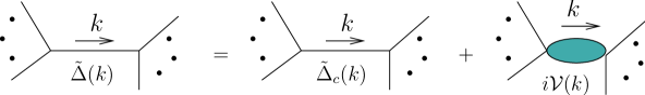
In the case of nonlocal interactions, however, the sum in (5.12) is an infinite sum that no longer can be removed by a finite number of local counterterms. The contact terms now sum up to a transcendental entire function, a nonlocal contribution that cannot be dropped: the non-polynomial asymptotic behavior renders the propagator , given by (5.3), not equal to the causal propagator given by (5.10). By the same token a (appropriately subtracted) Kallén-Lehmann representation cannot be obtained for (5.3). Note in this connection that in the expression (5.12) for the quantity
involves the field commutator Fourier transform , which, however, upon integration will not vanish for spacelike distances due to the presence of the factors. In momentum space (5.12) is given by
as the convergent expansion in positive powers of an entire function. Thus, manifestly does not contribute to absorptive parts and can in fact be viewed as a nonlocal vertex (Figure 3).
In the case of kernels of bounded support the following observation can now be made. If in (5.8), then one necessarily has . Hence
| (5.16) | |||||
Thus, in coordinate space, the difference between and the causal propagator, i.e. , , arises entirely from inside the bounded region of the kernel support and its effect is confined in it. In momentum space, since for sufficiently small , is essentially constant for all less than of order , and is of rapid decay for , it is evident from (5.2) that is appreciably nonvanishing only for momenta of order . Note how the (classical) picture of evolution over time-blocks of size in the section 4 accords with these quantum propagation properties.
Having examined the structure of the propagator we may now consider the conditions imposed on amplitudes by causality.
5.2.1 Local interaction
It will be useful to first recall the local case. The general causality condition is the Bogoliubov causality condition [21], [22]. It can be stated, in various slightly different but equivalent versions, in terms of amplitudes and thus in terms of diagrams. (Conditions on -point Wightman functions under appropriate permutations of their arguments, a special case of which is the frequently stated condition of commutativity of field operators at spacelike distances, reduce, when diagrammatically expressed, to special versions of the Bogoliubov conditions.)
In the local interaction case the propagators are given by (5.1), (5.5) and (5.6) with local vertex factors . Following [23], [15] we conveniently state the Bogolyubov causality condition in the form:
![[Uncaptioned image]](/html/1507.00981/assets/x4.png)
| (5.17) |
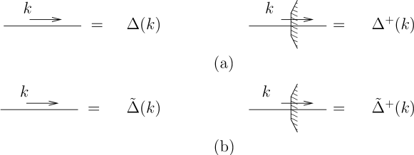
Here the blob represents any given diagram or collection of diagrams with a given number of external legs. The external vertices, labeled 1 and 2, to which two or more of these legs are attached, have been selected and explicitly indicated; nothing else is depicted explicitly, see Fig. 4 (a). Vertices 1 and 2 may be any interaction vertices present in the Lagrangian or represent the insertion of operators used to probe the process. The broken line arises from the momentum space representation of theta functions introduced for time-ordering vertices 1 and 2 in the coordinate space statement of the condition [21]; it amounts to a (non-covariant) propagator connecting the two vertices given in Fig. 4 (b).

The shaded lines in (5.17) represent the sum over all Cutkosky cuts placed in the manner indicated. Energy flows from the unshaded to the shaded side, each cut propagator being replaced by (Fig. 5(a)).
Because energy is conserved at vertices a region on the unshaded side must be connected to incoming lines, and a region on the shaded sided to outgoing lines. On the shaded side Feynman rules are those of , i.e., complex conjugated propagators and vertex factors. Thus, the second term represents the sum over all Cutkoski cuts with vertices 1 and 2 on the unshaded side; the sum in the third term is over cuts with vertex 2 on the shaded side and vertex 1 on the unshaded side. An efficient derivation proceeds from the Veltman largest time equation which employs the representation (5.5) leading to general cutting formulas for any (set of) graph(s) [23]. (5.17)) is then obtained as a particular application of these cutting formulas.121212The unitarity equations expressing the absorptive parts as a sum over Cutkosky cuts can also be obtained as another application of these cutting formulas. The well-known details are given in [23] , [15].
5.2.2 Nonlocal interaction
In the presence of nonlocal interactions (5.5) is replaced by (5.9). The presence of means that the derivation leading to (5.17) no longer holds. To obtain an appropriate extension of (5.17) in the nonlocal case we proceed as follows. Start with the causal propagator given by (5.10) - (5.11). Using this causal propagator the derivation leading to (5.17) now applies, and one regains (5.17) but now with propagators and cut lines . (Incidentally, this would be the BCC equation for nonzero spin fields and/or local derivative interactions, i.e., cases with appropriate polynomial , as discussed above.) We next substitute for each propagator. In this manner we obtain:
![[Uncaptioned image]](/html/1507.00981/assets/x7.png)
| (5.18) |
The l.h.s in (5.18) is as in (5.17) but now applied to the our nonlocal theory (2.2) - (2.3), i.e. all propagators are given by on the unshaded side and its complex conjugate on the shaded side, whereas all cut lines represent , cf. Fig. 5 (b). To each term on the l.h.s. there corresponds a set of reduced graphs, indicated by the insertion of the label , obtained by replacing its propagators (uncut internal lines) by the nonlocal vertex in all possible ways. A simple example is given in Fig. 6.
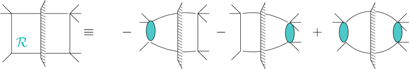
The r.h.s. in (5.18) then consists of summing over all such reduced graphs. (5.18) is our extension of the Bogoliubov causality equation in the presence of nonlocal interactions. The r.h.s. represents the corrections to the local theory condition (5.17) due to nonlocality.
In the case of quasi-local, i.e., bounded support interactions these corrections are generally extremely small since, as pointed above, a nonlocal vertex differs from zero essentially only around momenta of order . Of particular relevance are processes involving scales longer than the nonlocality scale . Except for internal momenta circulating in loops, momenta flowing through the diagram are below and the corresponding internal lines gives essentially zero contribution to the nonlocal vertex (5.2). It is natural in such a case to consider, in particular, the two external vertices 1 and 2 used to probe causality to be connected to the rest of the diagram by tree branches carrying momenta well below into the diagram. This would represent measurements over spacetime scales (much) larger than . Contributions from the nonlocal vertex in internal loops are small because of the rapid decay properties of cutting off momenta above - cf. remark following (5.16). The theory at scales longer than behaves essentially as a local theory with a cutoff . This may be viewed as providing the quantum underpinning of our remarks in the classical context in the latter part of section 3.2.
In the case of strictly nonlocal, i.e., unbounded support interactions characterized by some scale the noncausal effects can “leak” out of regions of size and be more or less pronounced depending on the form of the delocalization kernel . If decays exponentially outside a region of size , any non causal effects can be extremely small at large distances relative to . Such nonlocal interactions would be hardly distinguishable from quasi-local ones, at least as long as small acausal effects leaking out do not accumulate in some special processes.
6 Discussion and outlook
In summary, we studied scalar field theories with interactions of delocalized fields, the delocalization being specified through a nonlocal integral kernel . We imposed conditions on such kernels to insure UV finiteness and unitarity of amplitudes. Kernels satisfying such conditions are smooth functions of rapid decay and classified as either strictly nonlocal or quasi-local (bounded support) kernels. In the quantum theory this may be described as the kernels being chosen in the appropriate test function spaces that regularize the quantum fields (tempered distributions). Using this framework we gave a detailed treatment of the classical IVP. The introduction of nonlocal kernels results into partial integro-differential equations of motion and an IVP with past and future delays. We gave rigorous proofs of the existence but also the accompanying complete lack of uniqueness of solutions due to the future delays. This is, of course, the manifestation of acausality. We saw how the acausality effects are mitigated when confined in a region of limited extent. Passing to the quantum theory we derived a generalization of the equation for the Bogolyubov causality condition on amplitudes. This generalization, eq. (5.18), explicitly shows how the terms in the equation expressing causal propagation must be supplemented to include the effects of nonlocality.
As discussed in section 5 the structure of these acausal corrections is such that, for quasi-local kernels of length size , their effect is confined within regions of size . This is no longer true for strictly nonlocal kernels where the acausal effects leak out. But they can be very small for sufficiently (exponentially) fast decaying kernels. In this connection one may recall the example of the Lee-Wick prescription which, though unrelated to the nonlocal theories studied here, also entails acausal tails but generally falling off only as powers of the distance. They, nonetheless, apparently produce tiny effects [24], [25]. For strictly nonlocal interactions, however, the possibility always remains of devising certain processes where small acausal effects leaking out to longer distances may accumulate.
In any event our results indicate that quasi-local interactions are the most appealing. They possess the good UV behavior conferred by nonlocality while they mitigate acausal effects by actually confining them within the bounded support region of the kernels given by some characteristic scale . In fact, as we saw in the last section, for physics at momenta below a cutoff of order they essentially behave as local theories. Microscopic acausalities confined within a small length scale are not necessarily bad, and may even be desirable for certain applications, in particular, in the very early universe [25].
We dealt exclusively with scalar theories in this paper. Coupling to fermions would not appear to present any problems. Extension to include gauge interactions, however, is not straightforward. This is because gauge invariance relates the interaction and the free parts of the action. Thus, they no longer can be independently modified without breaking the invariance. In particular, one can not delocalize just the interactions. One approach is to delocalize gauge invariant or covariant field combinations such as or . This is the approach followed in [3], also [5], [6]. It typically results in superrenormalizability rather than complete UV finiteness, as was already realized in the early work on nonlocal QED [1]. Another approach [26] is to first do modify the interactions, thus breaking gauge invariance, and then try to restore it by the iterative addition of an infinite series of new interaction terms to the action. Such constructions, though, are rather unwieldy and of doubtful action convergence properties, and have not been completely carried out explicitly. These, however, are not the only possible approaches for introducing nonlocality in gauge theories. Gravity, in particular, is special in the sense that the basic fields are tensors rather than connections, and this offers some additional possibilities, which we will consider elsewhere.
Returning to scalar fields, one may remark that, at least in the absence of supersymmetry, they are difficult to accommodate within the usual framework of local field theory, i.e., incorporate as non-trivial (non-perturbatively existing) theories. In that they may be somewhat similar to gravity (the other even-spin bosonic field). There is always an inherent, wide arbitrariness in the potential of scalar fields that may be only resolved by the presence of a non-Gaussian (Wilson-Fisher type) UV fixed point assuring existence. Nonlocality, which, as expounded above, can accommodate general potentials, may offer another way to accomplish this. It is in fact amusing that quasi-local interactions to some degree mimic the presence of an UV fixed point, as will be discussed elsewhere.
Finally, one might consider the deeper question of how delocalized fields such as those studied here may arise. In this paper we introduced a scalar density function on the spacetime manifold whose role is to delocalize fields. We then investigated the properties must possess and the behavior of the resulting theories of interacting delocalized fields in some detail. We did not inquire as to any possible physical basis or mechanisms underlying the presence of . Addressing this question would require a deeper theory.
References
- [1] R.P. Feynman, Phys. Rev. 74, 939 (1948); A. Pais and G. E. Uhlenbeck, Phys. Rev. 79, 145 (1950); P. Kristensen and C. Møller, Dan. Mat. Fys. Medd. 27, no. 7 (1952); W. Pauli, Nuovo Cimente, 10, 648 (1953); M. Ebel, Dan. Mat. Fys. Medd. 29, no. 2 (1954); M. Chrétien and R. E. Peierls, Nuovo Cimento 10, 668 (1953); M Crétien and R. Peierls, Proc. R. Soc. London A223, 468 (1954); C. Hayashi, Prog. Theor. Phys. 10, 533 (1953); ibid, 11, 226 (1954); N. Shono and N. Oda, Prog. Theor. Phys. 8, 28 (1952); F. Bopp, Ann. d. Physik, 42, 573 (1942); H. Mc Manus, Proc. R. Soc. London A195, 323 (1948); G. Wataghin, Z. Phys. 86, 92 (1934).
- [2] M. Meyman, Sov. Phys. JETP 20, 1320 (1965); . V. Efimov, Com. Math. Phys. 5, 42 (1967); ibid, 7, 138 (1968); M. Z. Iofa and V. Ya. Fainberg, Theor. Mat. Fiz. 1, 187 (1969); M. Z. Iofa and V. Ya. Fainberg,, Sov. Phys. JETP 29, 880 (1969); V. Ya. Fainberg and M. A. Soloniev, Ann. Phys. 113, 421 (1978); V. Ya. Feinberg and M. A. Soloviev, Theor. Math. Phys. 93, 1438 (1992).
- [3] E. T. Tomboulis, arXiv:hep-th/9702146.
- [4] T. Biswas, E. Gerwick, T. Koivisto and A. Mazumdar, Phys. Rev. Lett. 108, 031101 (2012) [arXiv:1110.5249].
- [5] T. Biswas, A. Conroy, A. S. Koshelev and A. Mazumdar, Class. Quant. Grav. 31, 015022 (2014) [arXiv:1308.2319].
- [6] L. Modesto, Phys. Rev. D 86, 044005 (2012).
- [7] L. Modesto, Astron. Rev. 8.2, 4 (2013) [arXiv:11202.3151]; L. Modesto, arXiv:1402.6795[hep-th]]; F. Briscese, L. Modesto and S. Tsujikawa, Phys. Rev. D 89, 024029 (2014) [arXiv:1308.1413]; G. Calcagni and L. Modesto, Phys. Rev. D 91, 124059 (12015) [arXiv:1404.2137 [hep-th]; L. Modesto and L. Rachwal, Nucl. Phys. B889, 228 (2014) [arXiv:1407.8036].
- [8] M. Isi, J. Mureika and P. Nocolini, JHEP 1311:139 (2013) [arXiv:1310.8153 [hep-th]].
- [9] V. P. Frolov, arXiv:1505.00492; V. P. Frolov, A. Zelnikov and T. de Paula Netto, arXiv:1504.00412.
- [10] N. Barnaby and N. Kamran, JHEP 0802, 008 (2008).
- [11] X. Jaén, J. Llosa and A. Molina, Phys. Rev. D 34, 2302 (1986).
- [12] D. A. Eliezer and R. P. Woodard, Nucl. Phys. B325, 389 (1989).
- [13] D. V. Prokhorenko [arXiv:math-ph/0611068]; V. Vladimirov, Theor. Math. Phys. 149, 1604 (2006) [Teor. Mat. Fiz. 149, 354 (2006)] [arXiv:0705.4600].
- [14] T. A. Burton, “Stability and periodic solutions of ordinary and functional differential equations”, Dover (2005).
- [15] G. ’t Hooft and M. Veltman, Diagrammar in Particle interactions at very high energies, D. Speiser, F. Halzen and J. Weyers, eds., Plenum Press (1974) [CERN Report 73-9]; M. Veltman, Diagrammatica, Cambdidge U. P. (1994).
- [16] I. M. Gel’fand and G. E. Shilov, Generalized functions, Vols. I, II, Academic Press (1964).
- [17] J. Shatah and M. Struwe, Geometric wave equations, American Mathematical Society (1998); T. Tao, Nonlinear dispersive equations, American Mathematical Society (2006).
- [18] K. Deimling, “Nonlinear functional analysis”, Springer (1985).
- [19] R. J. Eden, P.V. Landshoff, D. I. Olive and J. C. Polkinghorne, The analytic S-matrix, Cambridge U. P. (1966).
- [20] R. E. Cutkosky, J. Math. Phys., 1, 429 (1960).
- [21] N. N. Bogoliubov and D. V. Shirkov, Introduction to the theory of quantized fields, Wiley-Interscience (1959).
- [22] N. N. Bogoliubov and D. V. Shirkov, Fortschr. der Physik, 3, 439 (1955); N. N. Bogoliubov, B. Medvedev and M. Polivanov, ibid, 6, 169 (1958).
- [23] M. Veltman, Physica 29, 186 (1963).
- [24] R. E. Cutkosky, P. V. Landshoff, D. I. Olive and J. C. Polkinghorne, Nucl. Phys. B12, 281 (1969); B. Grinstein, D. O’Connell and M. B. Wise, Phys. Rev. D 79, 105019 (2009).
- [25] E. T. Tomboulis, Phys. Lett. 97B, 77 (1980).
- [26] D. Evens, J. W. Moffat, G. Kleppe and R. P. Woodard, Phys. Rev. D 43, 499 (1991); G. Kleppe and R. P. Woodard, Nucl. Phys. B388, 81 (1992); J. W. Moffat, Phys. Rev. D 41, 1177 (1990).