Modified atomic decay rate near absorptive scatterers at finite temperature

Abstract

The change in the decay rate of an excited atom that is brought about by extinction and thermal-radiation effects in a nearby dielectric medium is determined from a quantummechanical model. The medium is a collection of randomly distributed thermally-excited spherical scatterers with absorptive properties. The modification of the decay rate is described by a set of correction functions for which analytical expressions are obtained as sums over contributions from the multipole moments of the scatterers. The results for the modified decay rate as a function of the distance between the excited atom and the dielectric medium show the influence of absorption, scattering and thermal-radiation processes. Some of these processes are found to be mutually counteractive. The changes in the decay rate are compared to those following from an effective-medium theory in which the discrete scatterers are replaced by a continuum.

I Introduction

The emission process of a photon by an excited atom is influenced by its environment P46 ; D70 ; CPS74 . In particular, when the excited atom is located in the vicinity of a dielectric body, its decay rate will be different from that in vacuum. It will depend crucially on the precise properties of the dielectric medium for several reasons. Interference effects due to the reflection of emitted photons from the surface of a dielectric medium will alter the atomic decay rate. Furthermore, if the medium is dispersive and lossy, it may absorb photons. This absorption process will lead to an enhanced atomic decay. Scattering effects due to inhomogeneities in the dielectric medium will also change the atomic decay. Finally, if the dielectric has got a finite temperature, it will emit thermal radiation which will stimulate the emission process. All these effects will depend on the shape of the dielectric body and on its distance from the atom.

Detailed studies of the changes in the atomic decay rate due to the presence of homogeneous lossy dielectric media at zero temperature have been carried out for various geometries. The simplest case is that of a halfspace that is uniformly filled with a dispersive dielectric A75 ; YG96 ; SKW99 ; EZ12 . A more complicated configuration is that of a dielectric sphere, which has been studied extensively R82 ; AON83 ; KLG88 ; DKW00 ; DKW01 ; KL05 ; CLT12a ; CLT12b . Other geometries like cylinders or spheroids have been considered as well KDL01 .

In a realistic medium extinction of radiation is produced not only by absorption but also by scattering from inhomogeneities. Both these effects will alter the decay rate of a nearby atom. When the inhomogeneities are densely distributed, multiple-scattering effects greatly complicate the analysis. For such systems numerical simulations have been used to gain insight in modified emission processes YV07a ; YV07b ; FPCS07 ; PC10 . For a dilute distribution of scatterers, however, multiple scattering plays a minor role, so that analytical methods may be used. In a recent paper SvW11 we have studied a model in which an excited atom is situated near a halfspace that is filled with a dilute set of spherical scatterers consisting of absorptive dielectric material. For this model detailed results for the change in the atomic decay rate as a function of the distance between atom and halfspace have been obtained.

The changes in the atomic decay rate due to thermal radiation from a nearby dielectric medium are of a different nature from those discussed above, as they are a consequence of stimulated-emission effects. Although their origin is different, they are likewise sensitive to the geometric details of the dielectric medium. For a uniform medium with a flat interface thermal-radiation effects in the atomic emission process have been studied in SJCG00 ; JMMCG05 .

In the present paper we shall treat within a single model decay-rate changes due to both extinction effects (from absorption and scattering) and to thermal radiation. We shall consider a randomly distributed dilute set of spherical scatterers consisting of a lossy dielectric material. By choosing the scatterers to be spherical as in SvW11 we are able to use the framework provided by Mie theory. Taking the set of scatterers to be dilute permits us to neglect multiple-scattering effects, as explained above. The scatterers will be held at a finite temperature so that they will emit thermal radiation. We will choose the set of scatterers to be bounded, so that the optical depth of the aggregate stays finite. For analytical purposes, the shape of the aggregate will be taken to be spherical. The model will allow us to treat the effects of reflective interference, absorption, scattering and thermal radiation on an equal footing.

The paper is organized as follows. In Section II we introduce our model that is based on the damped-polariton formulation of absorptive dielectrics. We formulate the atomic decay rate in terms of the second moment of the electric field and the associated Green function. In Section III we use addition theorems for vectorial spherical wave functions to evaluate the correction functions that govern the changes in the atomic decay rate in the presence of a set of absorptive scatterers at finite temperature. Subsequently, an alternative approach to the correction functions is given in Section IV. It makes use of integral representations, which are more suitable for numerical evaluation. Some typical examples of the ensuing graphs for the correction functions are presented in Section V. Furthermore, a comparison is made with an effective-medium model in which a uniform dielectric replaces the set of discrete scatterers. In a final Section VI our results are summarized and discussed. A few technical details of our treatment are given in a set of Appendices.

II Atomic emission and absorption near a dispersive dielectric medium

A dispersive and absorptive linear dielectric medium may be described by a damped-polariton model that has been introduced some time ago HB92 . In this model damping effects are taken into account by coupling the polarization density to a bath of harmonic oscillators with a continuous range of frequencies. For a uniform dielectric medium Fourier expansions can be used to diagonalize the model Hamiltonian and to determine its eigenmodes. For arbitrarily inhomogeneous media diagonalization can likewise be carried out by means of a Green function technique SvW04 . In the latter case diagonalization leads to a Hamiltonian of the form

$$H=\int d\mathbf{r}\int_{0}^{\infty}d\omega\,\hbar\omega\,\mathbf{C}^{\dagger}(\mathbf{r},\omega)\cdot\mathbf{C}(\mathbf{r},\omega)\,,$$ (1)

with annihilation operators $\mathbf{C}(\mathbf{r},\omega)$ and associated creation operators depending on position and frequency arguments. These fulfill the standard commutation relations $[\mathbf{C}(\mathbf{r},\omega),\mathbf{C}^{\dagger}(\mathbf{r}^{\prime},\omega^{\prime})]=\textsf{{I}}\,\delta(\mathbf{r}-\mathbf{r}^{\prime})\delta(\omega-\omega^{\prime})$, with I the unit tensor. The electric field can be expressed in terms of these operators as $\mathbf{E}(\mathbf{r})=\int_{0}^{\infty}d\omega\,\mathbf{E}(\mathbf{r},\omega)+\mathrm{h.c.}$, with

$$\mathbf{E}(\mathbf{r},\omega)=\int d\mathbf{r}^{\prime}\,\textsf{{f}}_{E}(\mathbf{r},\mathbf{r}^{\prime},\omega)\cdot\mathbf{C}(\mathbf{r}^{\prime},\omega)\,.$$ (2)

The tensorial coefficient $\textsf{{f}}_{E}$ reads SvW04 :

$$\textsf{{f}}_{E}(\mathbf{r},\mathbf{r}^{\prime},\omega)=-i\,\frac{\omega^{2}}{c^{2}}\left[\frac{\hbar\,\mathrm{Im}\,\varepsilon(\mathbf{r}^{\prime},\omega+i0)}{\pi\varepsilon_{0}}\right]^{1/2}\,\textsf{{G}}(\mathbf{r},\mathbf{r}^{\prime},\omega+i0)\,.$$ (3)

Here $\varepsilon$ is the complex local (relative) dielectric constant, which follows from the parameters of the model. Furthermore, G is the tensorial Green function, which satisfies the differential equation

$$-\nabla\times[\nabla\times\textsf{{G}}(\mathbf{r},\mathbf{r}^{\prime},\omega+i0)]$$

$$+\frac{\omega^{2}}{c^{2}}\,\varepsilon(\mathbf{r},\omega+i0)\,\textsf{{G}}(\mathbf{r},\mathbf{r}^{\prime},\omega+i0)=\textsf{{I}}\,\delta(\mathbf{r}-\mathbf{r}^{\prime})\,.$$ (4)

The rate of photon emission by an excited atom in the vicinity of a dispersive and absorptive dielectric follows from the inhomogeneous damped-polariton model in its diagonalized form by employing perturbation theory in leading order and disregarding transient effects SvW10 . In the electric-dipole approximation it can be expressed as an integral over the second moment of the electric field:

$$\Gamma=\frac{2\pi}{\hbar^{2}}\langle e|{\bm{\mu}}|g\rangle\cdot\int_{0}^{\infty}d\omega^{\prime}\,\langle\mathbf{E}(\mathbf{r}_{a},\omega)\mathbf{E}^{\dagger}(\mathbf{r}_{a},\omega^{\prime})\rangle\cdot\langle g|{\bm{\mu}}|e\rangle\,,$$

(5)

with atomic dipole matrix elements connecting the excited state (labelled $e$) and the ground state ($g$) of the atom, with $\omega$ the atomic transition frequency and with $\mathbf{r}_{a}$ the atomic position. The second moment of the electric field is determined by the density matrix of the damped-polariton system.

After insertion of (2) one encounters the second moment of the creation and annihilation operators. This second moment will be assumed to be isotropic and diagonal in both the position and the frequency variables:

$$\langle\mathbf{C}(\mathbf{r},\omega)\,\mathbf{C}^{\dagger}(\mathbf{r}^{\prime},\omega^{\prime})\rangle=[1+g(\mathbf{r},\omega)]\,\textsf{{I}}\,\delta(\mathbf{r}-\mathbf{r}^{\prime})\delta(\omega-\omega^{\prime})\,,$$ (6)

with a real and positive function $g(\mathbf{r},\omega)$ that vanishes when the damped-polariton system, as given by the Hamiltonian (1), is in its ground state. The second moment of the electric field now gets the form

$$\langle\mathbf{E}(\mathbf{r},\omega)\mathbf{E}^{\dagger}(\mathbf{r},\omega^{\prime})\rangle=\delta(\omega-\omega^{\prime})\frac{\hbar\omega^{4}}{\pi\varepsilon_{0}c^{4}}$$

$$\times\int d\mathbf{r}^{\prime}\,\textsf{{G}}(\mathbf{r},\mathbf{r}^{\prime},\omega+i0)\cdot\tilde{\textsf{{G}}}^{\ast}(\mathbf{r},\mathbf{r}^{\prime},\omega+i0)$$

$$\times[1+g(\mathbf{r}^{\prime},\omega)]\,\mathrm{Im}\,\varepsilon(\mathbf{r}^{\prime},\omega+i0)\,,$$ (7)

with $\tilde{\textsf{{G}}}$ the transpose of G. The part of the integral that is independent of $g(\mathbf{r},\omega)$ can be rewritten with the help of the optical theorem for the Green function:

$$\int d\mathbf{r}^{\prime}\,\textsf{{G}}(\mathbf{r},\mathbf{r}^{\prime},\omega+i0)\cdot\tilde{\textsf{{G}}}^{\ast}(\mathbf{r},\mathbf{r}^{\prime},\omega+i0)\,\mathrm{Im}\,\varepsilon(\mathbf{r}^{\prime},\omega+i0)=$$

$$=-\frac{c^{2}}{\omega^{2}}\,\mathrm{Im}\,\textsf{{G}}(\mathbf{r},\mathbf{r},\omega+i0)\,.$$ (8)

To evaluate the second part of the integral in (7) one needs information on the function $g(\mathbf{r}^{\prime},\omega)$ in the integrand. If $g(\mathbf{r}^{\prime},\omega)$ stays finite for large $|\mathbf{r}|^{\prime}$, the distant regions in the integral may contribute even when $\mathrm{Im}\,\varepsilon$ tends to 0 there. The importance of the far parts of space while evaluating the second moment of the electric field has been discussed previously HR09 . In fact, the Green function $\textsf{{G}}(\mathbf{r},\mathbf{r}^{\prime},\omega+i0)$ for a system with a uniform dielectric constant $\varepsilon$ at large distances from the origin will be proportional to $e^{i\omega\varepsilon|\mathbf{r}^{\prime}|/c}/|\mathbf{r}^{\prime}|$ for large $|\mathbf{r}^{\prime}|$, so that upon integration these distant regions yield a finite contribution even when $\mathrm{Im}\,\varepsilon$ gets negligibly small. However, if $g(\mathbf{r}^{\prime},\omega)$ tends to 0 for large $|\mathbf{r}^{\prime}|$, as is reasonable when no incoming fields are present, the contribution of the far spatial domain to the integral is no longer important when $\mathrm{Im}\,\varepsilon$ gets small there. In that case the integration in the second part of the integral in (7) can be confined to positions in space where $\mathrm{Im}\,\varepsilon$ differs from zero by a physically relevant amount, as will be indicated by a subscript $V$ at the integral. Upon assuming moreover for simplicity that both $g(\mathbf{r}^{\prime},\omega)$ and $\mathrm{Im}\,\varepsilon(\mathbf{r}^{\prime},\omega+i0)$ are independent of position within $V$, we arrive at the following expression for the second moment of the electric field:

$$\langle\mathbf{E}(\mathbf{r},\omega)\mathbf{E}^{\dagger}(\mathbf{r},\omega^{\prime})\rangle=-\delta(\omega-\omega^{\prime})\frac{\hbar\omega^{2}}{\pi\varepsilon_{0}c^{2}}\,\mathrm{Im}\,\textsf{{G}}(\mathbf{r},\mathbf{r},\omega+i0)$$

$$+\delta(\omega-\omega^{\prime})\frac{\hbar\omega^{4}}{\pi\varepsilon_{0}c^{4}}g(\omega)\,\left[\mathrm{Im}\,\varepsilon(\omega+i0)\right]$$

$$\times\int_{V}d\mathbf{r}^{\prime}\textsf{{G}}(\mathbf{r},\mathbf{r}^{\prime},\omega+i0)\cdot\tilde{\textsf{{G}}}^{\ast}(\mathbf{r},\mathbf{r}^{\prime},\omega+i0)\,.$$ (9)

For a dielectric at a finite inverse temperature $\beta$ one may insert $g(\omega)=1/(e^{\beta\hbar\omega}-1)$.

The atomic decay rate follows by substituting (9) in (5). As a result the decay rate is found as the sum of two terms, one representing spontaneous emission in the presence of an absorbing dielectric at zero temperature, and the other a correction describing stimulated emission due to the finite-temperature radiation from the dielectric. These two contributions have different properties and should be treated separately, as has been remarked before SJCG00 ; SSG02 ; HR09 .

In the presence of thermal radiation from the dielectric, atomic transitions from the ground state to the excited state may occur as well. The ensuing rate of atomic absorption is determined by an expression similar to (5):

$$\Gamma_{\mathrm{a}}=\frac{2\pi}{\hbar^{2}}\langle g|{\bm{\mu}}|e\rangle\cdot\int_{0}^{\infty}d\omega^{\prime}\,\langle\mathbf{E}^{\dagger}(\mathbf{r}_{a},\omega)\mathbf{E}(\mathbf{r}_{a},\omega^{\prime})\rangle\cdot\langle e|{\bm{\mu}}|g\rangle\,.$$

(10)

The second moment of the electric field occurring here is given by the analogue of (9), with no first term and with a second term that follows by interchanging G and $\textsf{{G}}^{\ast}$.

III Decay near a sphere with absorptive scatterers

We consider a spherical domain with radius $R$ that contains a dilute set of non-overlapping spherical scatterers with radii $a\ll R$ and complex dielectric constant $\varepsilon$, while the space between the scatterers is empty vacuum. The region $V$ in (9) is given by the union of the interiors of the spherical scatterers. The enveloping spherical domain with volume $4\pi R^{3}/3$ will be indicated by $V_{0}$. The scatterers are assumed to be randomly distributed with a uniform average density. An excited atom is located outside the spherical domain, at a distance $r_{a}>R+a$ from its center, which is chosen as the origin of a spherical coordinate system. We wish to determine the change in the decay rate that is brought about by the presence of the set of spherical scatterers. In this section we will first concentrate on the effects of scattering for the case of cold scatterers. Subsequently, finite-temperature effects will be considered as well.

For cold scatterers the second moment of the electric field is given by the first term of (9). For a single cold scatterer the Green function G is the sum of a vacuum contribution $\textsf{{G}}_{0}$ and a scattering term $\textsf{{G}}_{\mathrm{s}}$, as given in Appendix A. The imaginary part of the vacuum Green function with coinciding position arguments is proportional to the unit tensor: $\mathrm{Im}\,\textsf{{G}}_{0}(\mathbf{r},\mathbf{r},\omega+i0)=-\omega\textsf{{I}}/(6\pi c)$, whereas the imaginary part of the scattering term $\textsf{{G}}_{\mathrm{s}}$ for coinciding positions follows from (58).

For a dilute set of $N_{s}$ scatterers, with centers at the positions $\mathbf{r}_{i}$, the Green function can be approximated as

$$\textsf{{G}}(\mathbf{r},\mathbf{r}^{\prime},\omega+i0)=\textsf{{G}}_{0}(\mathbf{r},\mathbf{r}^{\prime},\omega+i0)$$

$$+\sum_{i}\textsf{{G}}_{\mathrm{s}}(\mathbf{r}-\mathbf{r}_{i},\mathbf{r}^{\prime}-\mathbf{r}_{i},\omega+i0)\,,$$ (11)

as follows by suppressing all terms involving multi-scatterer configurations in the Foldy-Lax equations or, more directly, in the Neumann series for the integral equation that determines the Green function TKS85 ; TK01 . Adopting this form of the Green function implies that multiple-scattering effects are henceforth neglected, as is reasonable for a dilute set. Since the centers of the scattering spheres are located at random positions inside the spherical domain with radius $R$, the configurational average of the second term of (11) may be written as an integral over $V_{0}$:

$$n_{s}\int_{V_{0}}d\mathbf{r}^{\prime\prime}\textsf{{G}}_{\mathrm{s}}(\mathbf{r}-\mathbf{r}^{\prime\prime},\mathbf{r}^{\prime}-\mathbf{r}^{\prime\prime},\omega+i0)\,,$$ (12)

with $n_{s}=3N_{s}/(4\pi R^{3})$ the density of the scatterers. Upon inserting the expression (58) for $\textsf{{G}}_{\mathrm{s}}$, employing the addition theorem (63) for the vector spherical wave functions $\mathbf{M}^{(h)}_{l,m}(\mathbf{r})$, $\mathbf{N}^{(h)}_{l,m}(\mathbf{r})$ and carrying out the integral over $\mathbf{r}^{\prime\prime}$, we get for the imaginary part of the configurationally averaged Green function with coinciding position arguments:

$$\mathrm{Im}\,\langle\textsf{{G}}(\mathbf{r},\mathbf{r},\omega+i0)\rangle=-\frac{\omega}{6\pi c}\textsf{{I}}+4\pi\frac{\omega}{c}n_{s}\sum_{l=1}^{\infty}l(l+1)$$

$$\times\sum_{l^{\prime}=1}^{\infty}\sum_{m^{\prime}=-l^{\prime}}^{l^{\prime}}\sum_{l^{\prime\prime}=0}^{\infty}(-1)^{m^{\prime}}\frac{2l^{\prime\prime}+1}{l^{\prime}(l^{\prime}+1)}I_{l^{\prime\prime}}(R)\left(\begin{array}[]{ccc}l&l^{\prime}&l^{\prime\prime}\\ 1&-1&0\end{array}\right)^{2}$$ (15)

$$\times\mathrm{Re}\left[(-i)^{l+1}B^{e}_{l}\left\{\delta^{\mathrm{e}}_{l+l^{\prime}+l^{\prime\prime}}\mathbf{N}^{(h)}_{l^{\prime},m^{\prime}}(\mathbf{r})\mathbf{N}^{(h)}_{l^{\prime},-m^{\prime}}(\mathbf{r})\right.\right.$$

$$\left.+\delta^{\mathrm{o}}_{l+l^{\prime}+l^{\prime\prime}}\mathbf{M}^{(h)}_{l^{\prime},m^{\prime}}(\mathbf{r})\mathbf{M}^{(h)}_{l^{\prime},-m^{\prime}}(\mathbf{r})\right\}$$

$$+(-i)^{l+1}B^{m}_{l}\left\{\delta^{\mathrm{e}}_{l+l^{\prime}+l^{\prime\prime}}\mathbf{M}^{(h)}_{l^{\prime},m^{\prime}}(\mathbf{r})\mathbf{M}^{(h)}_{l^{\prime},-m^{\prime}}(\mathbf{r})\right.$$

$$\left.\left.+\delta^{\mathrm{o}}_{l+l^{\prime}+l^{\prime\prime}}\mathbf{N}^{(h)}_{l^{\prime},m^{\prime}}(\mathbf{r})\mathbf{N}^{(h)}_{l^{\prime},-m^{\prime}}(\mathbf{r})\right\}\right]\,.$$ (16)

Here $I_{l}(R)=\int_{0}^{R}dr\,r^{2}[j_{l}(kr)]^{2}$, with $k=\omega/c$, results from the integration over the spherical domain. Its explicit form is

$$I_{l}(R) = {\textstyle\frac{1}{2}}R^{3}[j_{l}(kR)]^{2}+{\textstyle\frac{1}{2}}R^{3}[j_{l+1}(kR)]^{2}$$ (17)

$$-{\textstyle\frac{1}{2}}(2l+1)(R^{2}/k)j_{l}(kR)j_{l+1}(kR)\,,$$

as may be checked by differentiating with respect to $R$ and employing the recursion relations for the spherical Bessel functions NIST10 . The Wigner 3$j$-symbols in (16) imply that the three summation variables $l,l^{\prime},l^{\prime\prime}$ satisfy the triangular conditions $|l^{\prime}-l^{\prime\prime}|\leq l\leq l^{\prime}+l^{\prime\prime}$. Furthermore, $\delta^{\mathrm{e}}_{l}$ equals 1 for even $l$, and 0 for odd $l$, while $\delta^{\mathrm{o}}_{l}$ is defined analogously, with even and odd interchanged.

Substitution of (16) in the first term of (9) yields an expression for the configurational average of the second moment of the electric field. From the spherical symmetry it follows that the resulting tensor is diagonal in a spherical coordinate system with origin at the center of the aggregate of scatterers. Upon using the expressions for the vector spherical wave functions in spherical coordinates FJ87 one gets

$$\langle\!\langle\mathbf{E}(\mathbf{r},\omega)\mathbf{E}^{\dagger}(\mathbf{r},\omega^{\prime})\rangle\!\rangle=\delta(\omega-\omega^{\prime})\frac{\hbar\omega^{3}}{6\pi^{2}\varepsilon_{0}c^{3}}$$

$$\times\left\{\left[1+fF_{\mathrm{c},\parallel}(r)\right]\,\mathbf{e}_{r}\mathbf{e}_{r}+\left[1+fF_{\mathrm{c},\perp}(r)\right]\,\left(\mathbf{e}_{\theta}\mathbf{e}_{\theta}+\mathbf{e}_{\varphi}\mathbf{e}_{\varphi}\right)\right\}\,,$$

(18)

with the combined configurational and density-matrix average indicated by double brackets. Furthermore, $\mathbf{e}_{r}$, $\mathbf{e}_{\theta}$ and $\mathbf{e}_{\varphi}$ are unit vectors in spherical coordinates, and $f={\textstyle\frac{4}{3}}\pi a^{3}n_{s}$ is the filling fraction of the spherical domain containing the scatterers. The decay-rate correction functions $F_{\mathrm{c},\parallel}$ and $F_{\mathrm{c},\perp}$ are

$$F_{\mathrm{c},\parallel}(r)=-\frac{9}{2a^{3}}\sum_{l=1}^{\infty}l(l+1)\sum_{l^{\prime}=1}^{\infty}\sum_{l^{\prime\prime}=0}^{\infty}l^{\prime}(l^{\prime}+1)c_{l,l^{\prime}.l^{\prime\prime}}(R)$$

$$\times\mathrm{Re}\left[(-i)^{l+1}\left(B^{e}_{l}\delta^{\mathrm{e}}_{l+l^{\prime}+l^{\prime\prime}}+B^{m}_{l}\delta^{\mathrm{o}}_{l+l^{\prime}+l^{\prime\prime}}\right)\frac{1}{k^{2}r^{2}}\,H_{l^{\prime}}(kr)\right]\,,$$

(19)

$$F_{\mathrm{c},\perp}(r)=-\frac{9}{4a^{3}}\sum_{l=1}^{\infty}l(l+1)\sum_{l^{\prime}=1}^{\infty}\sum_{l^{\prime\prime}=0}^{\infty}c_{l,l^{\prime}.l^{\prime\prime}}(R)$$

$$\times\mathrm{Re}\biggl{[}(-i)^{l+1}\left(B^{e}_{l}\delta^{\mathrm{e}}_{l+l^{\prime}+l^{\prime\prime}}+B^{m}_{l}\delta^{\mathrm{o}}_{l+l^{\prime}+l^{\prime\prime}}\right)\frac{1}{k^{2}r^{2}}\,\bar{H}_{l^{\prime}}(kr)\biggr{.}$$

$$\left.+(-i)^{l+1}\left(B^{e}_{l}\delta^{\mathrm{o}}_{l+l^{\prime}+l^{\prime\prime}}+B^{m}_{l}\delta^{\mathrm{e}}_{l+l^{\prime}+l^{\prime\prime}}\right)H_{l^{\prime}}(kr)\right]\,,$$

(20)

with the functions $H_{l}(t)=[h^{(1)}_{l}(t)]^{2}$ and $\bar{H}_{l}(t)=[d[th^{(1)}_{l}(t)]/dt]^{2}$, and with the coefficients

$$c_{l,l^{\prime},l^{\prime\prime}}(R)=(2l^{\prime}+1)(2l^{\prime\prime}+1)I_{l^{\prime\prime}}(R)\left(\begin{array}[]{ccc}l&l^{\prime}&l^{\prime\prime}\\ 1&-1&0\end{array}\right)^{2}\,.$$ (21)

In view of (5) the average decay rate for an excited atom in the presence of a randomly distributed set of cold spherical scatterers can be written as

$$\langle\Gamma_{\mathrm{c}}\rangle=\Gamma_{0}+f\left[F_{\mathrm{c},\parallel}(r_{a})\Gamma_{0,\parallel}+F_{\mathrm{c},\perp}(r_{a})\Gamma_{0,\perp}\right]\,,$$ (22)

with the vacuum decay rate $\Gamma_{0}=\Gamma_{0,\parallel}+\Gamma_{0,\perp}$ for $\Gamma_{0,\parallel}=\omega^{3}|\langle e|{\bm{\mu}}\cdot\mathbf{e}_{r}|g\rangle|^{2}/(3\pi\varepsilon_{0}\hbar c^{3})$ and $\Gamma_{0,\perp}=\omega^{3}(|\langle e|{\bm{\mu}}\cdot\mathbf{e}_{\theta}|g\rangle|^{2}+|\langle e|{\bm{\mu}}\cdot\mathbf{e}_{\varphi}|g\rangle|^{2})/(3\pi\varepsilon_{0}\hbar c^{3})$. This expression for the decay rate in the presence of an aggregate of cold scatterers reduces to a simpler form if only a single scatterer is present. The latter form is found by taking the limit $R\rightarrow 0$ and $n_{s}\rightarrow\infty$ with $4\pi R^{3}n_{s}/3=1$, so that $n_{s}\,c_{l,l^{\prime},l^{\prime\prime}}(R)$ gets equal to $\delta_{l,l^{\prime}}\delta_{l^{\prime\prime},0}/(4\pi)$. As a consequence, only the terms with $\delta^{\mathrm{e}}_{l+l^{\prime}+l^{\prime\prime}}$ in the correction functions survive in this limit. The resulting expressions agree with those given in AON83 ; KLG88 ; DKW01 .

For the general case involving a collection of scatterers the decay-rate correction functions $F_{\mathrm{c},\parallel}$ and $F_{\mathrm{c},\perp}$ show a symmetry in the contributions of the electric and magnetic multipole amplitudes. This symmetry gets lost for a single scatterer. Both correction functions depend on the distance $r_{a}$ of the atom from the center of the spherical domain containing the scatterers, and parametrically on the radius $R$ of the spherical domain and on the radii $a$ of the scatterers themselves (through the scattering amplitudes $B^{e}_{l}$ and $B^{m}_{l}$). These three independent length scales that together characterize the configuration (all measured in terms of the wavelength of the atomic transition) occur neatly separated in the summands in (19) and (20). In particular, the dependence on $r_{a}$ is given by the spherical Hankel functions $h^{(1)}_{l^{\prime}}(kr_{a})$ and their derivatives. Since these are proportional to $e^{ikr_{a}}$, the correction functions will be oscillating as a function of $r_{a}$ (on the scale of the wavelength). For large $r_{a}$ the correction functions will decay to 0.

When the scatterers are taken to be at finite temperature the second moment of the electric field gets an additional contribution that is given by the second term in (9). The integral over $V$ in that term is taken over all positions $\mathbf{r}^{\prime}$ inside the scatterers, so that it is in fact a sum over individual contributions for each of the scatterers. As the system of scatterers is dilute, one may use the expression (70) for the Green functions in the integrand. In this way the hot-scatterer contribution to the second moment becomes

$$\delta(\omega-\omega^{\prime})\frac{\hbar\omega^{4}}{\pi\varepsilon_{0}c^{4}(e^{\beta\hbar\omega}-1)}\left[\mathrm{Im}\,\varepsilon(\omega+i0)\right]\sum_{i}\int_{|\mathbf{r}^{\prime}-\mathbf{r}_{i}|<a}d\mathbf{r}^{\prime}$$

$$\times\textsf{{G}}_{0\mathrm{s}}(\mathbf{r}-\mathbf{r}_{i},\mathbf{r}^{\prime}-\mathbf{r}_{i},\omega+i0)\cdot\tilde{\textsf{{G}}}^{\ast}_{0\mathrm{s}}(\mathbf{r}-\mathbf{r}_{i},\mathbf{r}^{\prime}-\mathbf{r}_{i},\omega+i0)\,.$$

(23)

When the explicit expression (70) for $\textsf{{G}}_{0\mathrm{s}}$ is substituted, the integration over $\mathbf{r}^{\prime}$ leads to three-dimensional integrals of scalar products of vector spherical wave functions of the form (72)–(74). The resulting integrals $I^{(\varepsilon)}_{l}(a)$ may be eliminated with the help of (76)–(77). Furthermore, the sum over $i$ may be replaced by an integral over positions $\mathbf{r}^{\prime\prime}$ inside the spherical domain of radius R. In this way we get from (23):

$$\delta(\omega-\omega^{\prime})\frac{\hbar\omega^{3}}{\pi\varepsilon_{0}c^{3}(e^{\beta\hbar\omega}-1)}n_{s}\int_{V_{0}}d\mathbf{r}^{\prime\prime}\sum_{l=1}^{\infty}\sum_{m=-l}^{l}\frac{1}{2l+1}$$

$$\times\left[C^{m}_{l}\mathbf{M}^{(h)}_{l,m}(\mathbf{r}-\mathbf{r}^{\prime\prime})\mathbf{M}^{(h)\ast}_{l,m}(\mathbf{r}-\mathbf{r}^{\prime\prime})\right.$$

$$\left.+C^{e}_{l}\mathbf{N}^{(h)}_{l,m}(\mathbf{r}-\mathbf{r}^{\prime\prime})\mathbf{N}^{(h)\ast}_{l,m}(\mathbf{r}-\mathbf{r}^{\prime\prime})\right]\,.$$ (24)

The remaining vector spherical wave functions, which depend on $\mathbf{r}-\mathbf{r}^{\prime\prime}$, can be rewritten by using the addition theorem of Appendix A. Finally, we arrive at an expression for the second moment that is a generalization of (18), with the cold-scatterer decay-rate corrections functions $F_{\mathrm{c},p}(r)$ (with $p=\,\parallel,\perp$) replaced by new functions $F_{p}(r)$. These contain, apart from the cold-scatterer correction functions, additional terms that arise when the dielectric medium in the scatterers emits thermal radiation. In fact, they have the form $F_{p}(r)=F_{\mathrm{c},p}(r)+(e^{\beta\hbar\omega}-1)^{-1}\,F_{\mathrm{d},p}(r)$, with the ‘dielectric’ decay-rate correction functions $F_{\mathrm{d},\parallel}(r)$ and $F_{\mathrm{d},\perp}(r)$. (The subscript $\mathrm{d}$ points to the fact that the hot-scatterer contributions find their origin in the dielectric medium.) The dielectric decay-rate correction functions have a similar form as (19) and (20), with the following differences: 1. the functions $H_{l}(t)$ and $\bar{H}_{l}(t)$ are replaced by $H_{\mathrm{d},l}(t)=|h^{(1)}_{l}(t)|^{2}$ and $\bar{H}_{\mathrm{d},l}(t)=|d[th^{(1)}_{l}(t)]/dt|^{2}$, respectively; 2. the multipole amplitudes $(-i)^{l+1}\,B^{q}_{l}$ (with $q=e,m$) are replaced by $-C^{q}_{l}$, defined in (78); 3. the symbol $\mathrm{Re}$ can be omitted (after the above changes the functions are real).

The average decay rate $\langle\Gamma\rangle$ for an excited atom in the presence of an aggregate of randomly distributed spherical scatterers at finite temperature gets the form:

$$\langle\Gamma\rangle=\Gamma_{0}+f\left[F_{\parallel}(r_{a})\Gamma_{0,\parallel}+F_{\perp}(r_{a})\Gamma_{0,\perp}\right]\,,$$ (25)

instead of (22). As we have seen in Section II, the cold-scatterer contribution to the average decay rate follows from the first term in (9), which resulted by rewriting part of the integral in (7) by means of the optical theorem (8). Hence, it originates from positions $\mathbf{r}^{\prime}$ both in the scatterers and in the surrounding space. In contrast, the hot-scatterer contribution has been obtained from the second term in (9), which is an integral over the volume $V$ occupied by the dielectric medium within the scatterers. To show more clearly the origin of the various contributions we may rearrange the total decay-rate correction functions $F_{p}$ by writing $F_{\mathrm{c},p}$ as the sum $F_{\mathrm{d},p}+F_{\mathrm{r},p}$ of the dielectric decay-rate correction function $F_{\mathrm{d},p}$ and a ‘radiative’ decay-rate correction function $F_{\mathrm{r},p}=F_{\mathrm{c},p}-F_{\mathrm{d},p}$, so that one gets

$$F_{p}(r)=F_{\mathrm{r},p}(r)+\frac{e^{\beta\hbar\omega}}{e^{\beta\hbar\omega}-1}F_{\mathrm{d},p}(r)\,,$$ (26)

with $p=\parallel,\perp$. In this form the last term contains all contributions from the dielectric medium within the scatterers (both for cold and for hot scatterers), whereas the first term represents radiative contributions associated to the space outside the scatterers.

The average absorption rate $\langle\Gamma_{\mathrm{a}}\rangle$ for a ground-state atom in the vicinity of a collection of randomly distributed hot scatterers can likewise be evaluated. As absorption and stimulated emission are closely related, it is found to be determined by the same correction functions $F_{\mathrm{d},\parallel}$ and $F_{\mathrm{d},\perp}$:

$$\langle\Gamma_{\mathrm{a}}\rangle=\frac{f}{e^{\beta\hbar\omega}-1}\left[F_{\mathrm{d},\parallel}(r_{a})\Gamma_{0,\parallel}+F_{\mathrm{d},\perp}(r_{a})\Gamma_{0,\perp}\right]\,.$$ (27)

The dielectric decay-rate correction functions for hot scatterers are quite analogous to their cold-scatterer counterparts (19) and (20). In particular, the symmetry between electric and magnetic multipole contributions is clearly visible in these functions as well. It gets lost in the limiting case of a single hot scatterer. As before, the independent length scales $r_{a}$, $R$ and $a$ show up in the summand. The dependence on $a$ is contained in the coefficients $C^{e}_{l}$ and $C^{m}_{l}$, while $R$ appears in the coefficients (21). The distance $r_{a}$ enters the summand through the absolute value of the spherical Hankel functions. As a consequence, the oscillating behavior found before is absent here. In fact, the dielectric correction functions will decay smoothly to 0 when the distance $r_{a}$ increases beyond bounds. In the next section we shall determine the precise form of the asymptotic behavior for all decay-rate correction functions.

IV Integral representations for the decay-rate correction functions

The expressions for the decay-rate correction functions as found in the previous section are three-fold sums of terms in which the independent variables $r_{a}$, $R$ and $a$ occur in separate factors. To determine their behavior as a function of $r_{a}$, for fixed values of the parameters $R$ and $a$, the sums have to be evaluated numerically. As it turns out, a greater numerical efficiency is achieved by starting from an alternative representation in which the variables $r_{a}$ and $R$ are intertwined in integral expressions. For cold scatterers such a representation can be found by starting again from the first term of (9) and using (11)-(12), as before. Upon choosing the atomic position $\mathbf{r}_{a}=\mathbf{r}=\mathbf{r}^{\prime}$ on the positive $z$-axis and inserting the representation (69), one may write the $zz$-component of the integrand in (12) as $\cos^{2}\chi\,G_{\mathrm{s},\parallel}(t,\omega+i0)+\sin^{2}\chi\,G_{\mathrm{s},\perp}(t,\omega+i0)$, with $t=|\mathbf{r}-\mathbf{r}^{\prime\prime}|$ and $\chi$ the angle between $\mathbf{r}-\mathbf{r}^{\prime\prime}$ and the positive $z$-axis. The integral over the azimuthal angle $\varphi^{\prime\prime}$ of $\mathbf{r}^{\prime\prime}$ is trivial now. The remaining double integral over the spherical variables $r^{\prime\prime}$ and $\theta^{\prime\prime}$ may be rewritten by introducing $t$ and $u=r^{\prime\prime}\cos\theta^{\prime\prime}$ as new integration variables, so that $\chi$ is determined by the relation $t\cos\chi=r-u$. The integration over $u$ can be carried out straightforwardly. After insertion of the components $G_{\mathrm{s},\parallel}$ and $G_{\mathrm{s},\perp}$ of the scattering Green function SvW11 , the $zz$-component of (12) leads to an expression for the second moment of the $z$-component of the electric field of the same form as in (18), with $F_{\mathrm{c},\parallel}(r)$ given as

$$F_{\mathrm{c},\parallel}(r)=-\frac{9}{8k^{3}a^{3}}\sum_{l=1}^{\infty}l(l+1)\mathrm{Re}\left[(-i)^{l+1}B^{e}_{l}J^{e}_{\mathrm{c},\parallel,l}(kr)\right.$$

$$\left.+(-i)^{l+1}B^{m}_{l}J^{m}_{\mathrm{c},\parallel,l}(kr)\right]\,.$$ (28)

The functions $J^{e}_{\mathrm{c},\parallel,l}$ and $J^{m}_{\mathrm{c},\parallel,l}$ are integrals over $t$:

$$J^{e}_{\mathrm{c},\parallel,l}(\zeta)=\int_{\zeta-\rho}^{\zeta+\rho}dt\,\frac{1}{t}\biggl{\{}\left[g_{1}(t,\zeta,\rho)-g_{2}(t,\zeta,\rho)\right]\bar{H}_{l}(t)\biggr{.}$$

$$\biggl{.}+2l(l+1)g_{2}(t,\zeta,\rho)H_{l}(t)\biggr{\}}\,,$$

(29)

$$J^{m}_{\mathrm{c},\parallel,l}(\zeta)=\int_{\zeta-\rho}^{\zeta+\rho}dt\,t\left[g_{1}(t,\zeta,\rho)-g_{2}(t,\zeta,\rho)\right]H_{l}(t)\,,$$

(30)

with $\rho=kR$. The auxiliary functions $g_{i}$ are

$$g_{1}(t,\zeta,\rho)=\frac{\rho^{2}-(\zeta-t)^{2}}{2\zeta}\,,$$ (31)

$$g_{2}(t,\zeta,\rho)=\frac{1}{3t^{2}}\left(\frac{\rho^{2}-\zeta^{2}-t^{2}}{2\zeta}\right)^{3}+\frac{1}{3}t\,,$$ (32)

while $H_{l}(t)$ and $\bar{H}_{l}(t)$ have been defined below (20).

Similarly, the $xx$-component of the integrand in (12) can be written as $\sin^{2}\chi\cos^{2}\varphi^{\prime\prime}\,G_{\mathrm{s},\parallel}(t,\omega+i0)+(\cos^{2}\chi\cos^{2}\varphi^{\prime\prime}+\sin^{2}\varphi^{\prime\prime})G_{\mathrm{s},\perp}(t,\omega+i0)$. Taking the same steps as above one arrives at an expression for the second moment of the $x$-component of the electric field as in (18). Here, $F_{\mathrm{c},\perp}(r)$ is found as

$$F_{\mathrm{c},\perp}(r)=-\frac{9}{16k^{3}a^{3}}\sum_{l=1}^{\infty}l(l+1)\mathrm{Re}\left[(-i)^{l+1}B^{e}_{l}J^{e}_{\mathrm{c},\perp,l}(kr)\right.$$

$$\left.+(-i)^{l+1}B^{m}_{l}J^{m}_{\mathrm{c},\perp,l}(kr)\right]\,,$$ (33)

with the integrals:

$$J^{e}_{\mathrm{c},\perp,l}(\zeta)=\int_{\zeta-\rho}^{\zeta+\rho}dt\,\frac{1}{t}\biggl{\{}\left[g_{1}(t,\zeta,\rho)+g_{2}(t,\zeta,\rho)\right]\biggr{.}\bar{H}_{l}(t)$$

$$\left.+2l(l+1)\left[g_{1}(t,\zeta,\rho)-g_{2}(t,\zeta,\rho)\right]H_{l}(t)\right\}\,,$$ (34)

$$J^{m}_{\mathrm{c},\perp,l}(\zeta)=\int_{\zeta-\rho}^{\zeta+\rho}dt\,t\left[g_{1}(t,\zeta,\rho)+g_{2}(t,\zeta,\rho)\right]H_{l}(t)\,.$$

(35)

For large $R$ the above results are consistent with those found previously SvW11 for the correction functions of the atomic decay rate in the vicinity of a halfspace. In fact, defining $\zeta^{\prime}=\zeta-\rho$ as the (scaled) distance from the atom to the surface of the spherical domain, one finds the asymptotic forms:

$$\lim_{\rho\rightarrow\infty}g_{1}(t,\zeta,\rho)=t-\zeta^{\prime}\quad,\quad\lim_{\rho\rightarrow\infty}g_{2}(t,\zeta,\rho)=\frac{1}{3}t-\frac{\zeta^{\prime 3}}{3t^{2}}\,.$$ (36)

Substituting these expressions into (29)–(30) and (34)–(35) one obtains decay-rate correction functions that are in agreement with the results of SvW11 .

For hot scatterers similar methods may be used to derive integral representations for $F_{\mathrm{d},\parallel}(r)$ and $F_{\mathrm{d},\perp}(r)$. To that end one starts from (23) and inserts the spherical-coordinate representations of the vector spherical wave functions in terms of the spherical variables $t,\chi,\varphi^{\prime\prime}$ defined above. Subsequently, one rewrites the triple integral over $\mathbf{r}^{\prime\prime}$ in terms of the integration variables $t,u,\varphi^{\prime\prime}$. Upon carrying out the integrals over the latter two variables one gets

$$F_{\mathrm{d},\parallel}(r)=\frac{9}{8k^{3}a^{3}}\sum_{l=1}^{\infty}l(l+1)\left[C^{e}_{l}J^{e}_{\mathrm{d},\parallel,l}(kr)\right.$$

$$\left.+C^{m}_{l}J^{m}_{\mathrm{d},\parallel,l}(kr)\right]\,,$$ (37)

$$F_{\mathrm{d},\perp}(r)=\frac{9}{16k^{3}a^{3}}\sum_{l=1}^{\infty}l(l+1)\left[C^{e}_{l}J^{e}_{\mathrm{d},\perp,l}(kr)\right.$$

$$\left.+C^{m}_{l}J^{m}_{\mathrm{d},\perp,l}(kr)\right]\,,$$ (38)

with integrals $J^{q}_{\mathrm{d},p,l}$ (for $p=\,\parallel,\perp$ and $q=e,m$) that follow from (29)-(30) and (34)-(35) by replacing $H_{l}(t)$ and $\bar{H}_{l}(t)$ with $H_{\mathrm{d},l}(t)$ and $\bar{H}_{\mathrm{d},l}(t)$, defined below (24). Hence, the expressions for the hot-scatterer integrals are quite similar to those for cold scatterers, with squares of moduli of spherical Hankel functions (and their derivatives) occurring instead of ordinary squares, as in the previous section.

The integral representations as given above are a suitable starting-point to derive the asymptotic behavior of the decay-rate correction functions for $r$ tending to $\infty$. When $r$ increases, the variable $\zeta=kr$ in the $J_{l}$-integrals (29)-(30) and (34)-(35) gets large. Hence, the integration variable $t$ in these integrals is large as well, so that one may insert the asymptotic form NIST10 of the spherical Hankel function $h^{(1)}_{l}(t)\simeq(-i)^{l+1}e^{it}/t$ and its derivative $d[th^{(1)}_{l}(t)]/dt\simeq(-i)^{l}e^{it}$ in the integrands. Instead of $t$ we now introduce the new integration variable $x$, by writing $t=\zeta+x$, so that the integration limits for $x$ become $\pm\rho$. For large $\zeta$ one may replace the combinations of $g_{1}$ and $g_{2}$ in the integrands by the leading terms in their power series in $1/\zeta$, at fixed values of $\rho$ and $x$. For instance, to determine the asymptotic form of (29) we write

$$\frac{1}{t}[g_{1}(t,\zeta,\rho)-g_{2}(t,\zeta,\rho)]\simeq(\rho^{2}-x^{2})^{2}/(4\zeta^{4})\,,$$ (39)

$$\frac{1}{t^{3}}g_{2}(t,\zeta,\rho)\simeq(\rho^{2}-x^{2})/(2\zeta^{4})\,.$$ (40)

Upon evaluating the (trivial) integral over $x$ we find:

$$J^{e}_{\mathrm{c},\parallel,l}(\zeta)\simeq(-1)^{l}\frac{e^{2i\zeta}}{\zeta^{4}}\left\{\left(-\frac{1}{2}\rho^{2}+\frac{3}{8}\right)\sin(2\rho)-\frac{3}{4}\rho\cos(2\rho)\right.$$

$$\left.-2l(l+1)\left[\frac{1}{4}\sin(2\rho)-\frac{1}{2}\rho\cos(2\rho)\right]\right\}\,$$ (41)

for large $\zeta$. In a similar way we get the asymptotic forms of the remaining cold-scatterer integrals for large $\zeta$:

$$J^{m}_{\mathrm{c},\parallel,l}(\zeta) \simeq(-1)^{l+1}\frac{e^{2i\zeta}}{\zeta^{4}}\left[\left(-\frac{1}{2}\rho^{2}+\frac{3}{8}\right)\sin(2\rho)\right.$$ (42)

$$\left.-\frac{3}{4}\rho\cos(2\rho)\right]\,,$$

$$J^{e}_{\mathrm{c},\perp,l}(\zeta) \simeq-J^{m}_{\mathrm{c},\perp,l}(\zeta)\simeq$$ (43)

$$\simeq(-1)^{l}\frac{e^{2i\zeta}}{\zeta^{2}}\left[\frac{1}{2}\sin(2\rho)-\rho\cos(2\rho)\right]\,.$$

The asymptotic decay-rate correction functions $F_{\mathrm{c},p}(r)$ (with $p=\,\parallel,\perp$) for cold scatterers, which follow by inserting the above asymptotic forms of the $J_{l}$-integrals in (28) and (33), are damped and oscillating, with a period of (half of) the wavelength. The damping is algebraic; it is proportional to $1/r^{4}$ for the longitudinal polarization, but slower, namely proportional to $1/r^{2}$, for the transverse polarization. For the latter polarization all contributions of the electric and magnetic multipoles are modulated by the same function of $\rho$ (or the radius $R$ of the spherical domain). Hence, when $\rho$ is a solution of the transcendental equation $\tan(2\rho)=2\rho$, the asymptotic form of $F_{\mathrm{c},\perp}(r)$ vanishes, which means that the decay is faster than $1/r^{2}$ in that case. Indeed, by evaluating the next order in the asymptotic expansion one finds a decay proportional to $1/r^{3}$ for these special values of $R$. Hence, the scatterers are less effective in modifying the atomic decay rate for these particular radii of the spherical domain.

For hot scatterers the asymptotic forms of the $J_{l}$-integrals can be determined in a similar fashion. Since only the absolute value of the spherical Hankel functions enter the integrands, no oscillations are found. One gets the following asymptotic results for large $\zeta$:

$$J^{e}_{\mathrm{d},\parallel,l}(\zeta) \simeq\frac{1}{\zeta^{4}}\left(\frac{4}{15}\rho^{5}+\frac{4}{3}l(l+1)\rho^{3}\right)\,,$$ (44)

$$J^{m}_{\mathrm{d},\parallel,l}(\zeta) \simeq\frac{4}{15}\frac{\rho^{5}}{\zeta^{4}}\,,$$ (45)

$$J^{e}_{\mathrm{d},\perp,l}(\zeta) \simeq J^{m}_{\mathrm{d},\perp,l}(\zeta)\simeq\frac{4}{3}\frac{\rho^{3}}{\zeta^{2}}\,.$$ (46)

The ensuing asymptotic forms of the dielectric decay-rate correction functions show a monotonously damped behavior proportional to $1/r^{4}$ and $1/r^{2}$ for the longitudinal and transverse polarizations, respectively.

For positions near the surface of the spherical domain containing the scatterers the decay-rate correction functions turn out to diverge. For cold scatterers and a longitudinal atomic polarization this follows by considering the integrals $J^{q}_{\mathrm{c},\parallel,l}(\zeta)$ (with $q=e,m$) for large $l$. Since for these values the spherical Hankel function gets the form $h^{(1)}_{l}(t)\simeq-i\,2^{l+1/2}\,l^{l}/(e^{l}\,t^{l+1})$ NIST10 , the integrals (29) and (30) can be evaluated explicitly. One gets:

$$J^{e}_{\mathrm{c},\parallel,l}(\zeta)\simeq-\frac{2^{2l}\,l^{2l}}{e^{2l}}\,\left[\frac{\rho}{\zeta(\zeta-\rho)^{2l+1}}-(\rho\rightarrow-\rho)\right]$$ (47)

and a similar form for $J^{m}_{\parallel,l}(\zeta)$, which is found to be proportional to $l^{2l-3}$ instead of $l^{2l}$. Hence, for increasing values of $l$ both integrals get large. However, in the correction function (28) these integrals are multiplied by the multipole amplitudes and summed over all $l$. For large $l$ the electric-multipole amplitude (as given by (59)) gets the asymptotic form

$$\mathrm{Re}\,\left[(-i)^{l+1}B^{e}_{l}\right]\simeq\frac{\mathrm{Im}\,\varepsilon(\omega+i0)}{|1+\varepsilon(\omega+i0)|^{2}}\frac{e^{2l}\,(ka)^{2l+1}}{2^{2l}\,l^{2l+2}}\,,$$ (48)

whereas the asymptotic form of the magnetic-multipole amplitude is proportional to $1/l^{2l+4}$. Upon inserting (47) and (48) into (28) and summing over $l$ one finds that the contributions of the electric multipoles diverge for $\zeta\rightarrow\rho-ka$, as it becomes a geometric series in $ka/(\zeta-\rho)$. In contrast, the contributions of the magnetic multipoles stay finite. As a result we obtain the following asymptotic form of the correction function $F_{\mathrm{c},\parallel}(r)$ for $r\rightarrow R+a$:

$$F_{\mathrm{c},\parallel}(r)\simeq\frac{9}{16k^{3}a^{2}}\frac{\mathrm{Im}\,\varepsilon(\omega+i0)}{|1+\varepsilon(\omega+i0)|^{2}}\frac{R}{(R+a)(r-R-a)}\,,$$ (49)

so that it diverges linearly near the surface of the spherical domain. Since the scattering spheres may protrude from the domain, the actual value of $r$ at which the correction function diverges is not $R$, but $R+a$.

The correction function for the transverse atomic polarization has a similar divergency, with a prefactor that is smaller by a factor of two: $F_{\mathrm{c},\perp}(r)\simeq{\textstyle\frac{1}{2}}F_{\mathrm{c},\parallel}(r)$. These asymptotic forms of the decay-rate correction functions for an atom near the surface of a spherical domain filled with cold scatterers are in agreement with those found for an atom near a halfspace with such scatterers SvW11 , as could have been expected.

Finally, we turn to the asymptotic expressions for the decay-rate correction functions pertaining to hot scatterers. Near the surface of the spherical domain containing the scatterers these are found to have the same divergency as those for cold scatterers: $F_{\mathrm{d},\parallel}(r)\simeq F_{\mathrm{c},\parallel}(r)$ and $F_{\mathrm{d},\perp}(r)\simeq F_{\mathrm{c},\perp}(r)$, for $r\rightarrow R+a$. The subdominant terms in the asymptotic expressions, which are proportional to $\log(r-R-a)$, are found to agree as well. As a consequence, the ‘radiative’ decay-rate correction functions $F_{\mathrm{r},\parallel}(r)$ and $F_{\mathrm{r},\perp}(r)$ stay finite near the surface of the domain.

The linearly divergent behavior of the decay-rate correction functions $F_{\mathrm{c},p}$ and $F_{\mathrm{d},p}$ (with $p=\parallel,\perp$) near the surface of a spherical domain filled with scatterers is less pronounced than that found for the atomic decay rate near a single homogeneous sphere DKW01 . In fact, the latter is proportional to $1/(r-a)^{3}$ for a sphere of radius $a$. The collective effect of an aggregate of scattering spheres is mitigated as a consequence of the configurational averaging, which implies a reduced probability for an individual scatterer to be near the atom even when $r_{a}$ is close to $R+a$.

V Evaluation of the decay-rate correction functions

The decay-rate correction functions $F_{\mathrm{c},\parallel}$ and$F_{\mathrm{c},\perp}$ for cold scatterers, as given by (28) and (33), depend on the distance $r$ via the integrals $J^{q}_{\mathrm{c},p,l}$, with $p=\,\parallel,\perp$ and $q=e,m$. Inspection of (29), (30), (34) and (35) shows that these integrals can be written as linear combinations of a set of basic integrals over the product of two spherical Hankel functions with an algebraic prefactor:

$$I_{l_{1},l_{2},n}(z)=\int^{z}du\,u^{-n}h^{(1)}_{l_{1}}(u)\,h^{(1)}_{l_{2}}(u)\,,$$ (50)

for $z>0$. As an example, one may write $J^{m}_{\mathrm{c},\parallel,l}$ as a linear combination of $I_{l,l,n}(z)$ with $n=-5,-3,-2,-1,1$ and $z=\zeta\pm\rho$. Clearly, only ‘diagonal’ basic integrals, with $l_{1}=l_{2}$, show up here. However, the arguments of the integrals $J^{e}_{\mathrm{c},\parallel,l}$ and $J^{e}_{\mathrm{c},\perp,l}$ in (29) and (34) contain both the square of a spherical Hankel function $h^{(1)}_{l}(t)$ and of the derivative $d[th^{(1)}_{l}(t)]/dt$. The latter may be rewritten in terms of a spherical Hankel function with a different order NIST10 , since one has $d[th^{(1)}_{l}(t)]/dt=(l+1)h^{(1)}_{l}(t)-th^{(1)}_{l+1}(t)$. As a consequence, upon rewriting $J^{e}_{\mathrm{c},\parallel,l}$ and $J^{e}_{\mathrm{c},\perp,l}$ in terms of basic integrals one encounters off-diagonal basic integrals with $l_{2}=l_{1}+1$ as well. It turns out that one needs information about the diagonal basic integrals $I_{l,l,n}(z)$ with $n=-5,-3,-2,-1,0,1,3$ and the off-diagonal integrals $I_{l,l+1,n}(z)$ with $n=-4,-2,-1,0,2$. All information about these basic integrals is collected in Appendix B.

For hot scatterers, the integrals $J^{q}_{\mathrm{d},p,l}$ (with $p=\,\parallel,\perp$ and $q=e,m$) may be analyzed in a similar way. They can be written as linear combinations of a second set of basic integrals containing the product of a spherical Hankel function and its complex conjugate:

$$I^{\prime}_{l_{1},l_{2},n}(z)=\int^{z}du\,u^{-n}h^{(1)}_{l_{1}}(u)\,[h^{(1)}_{l_{2}}(u)]^{\ast}\,.$$ (51)

Upon collecting all information about the integrals (50) and (51) we can derive explicit expressions for $J^{q}_{\mathrm{c},p,l}$ and $J^{q}_{\mathrm{d},p,l}$, for $p=\,\parallel,\perp$ and $q=e,m$. Combining these with the expressions for the electric and magnetic multipole amplitudes (59) we are able to draw curves for the decay-rate correction functions.

For cold scatterers and a transverse atomic polarization the decay-rate correction function $F_{\perp}=F_{\mathrm{c},\perp}$ is shown for a representative choice of $R$, $a$ and $\varepsilon$ in Fig. 1. As remarked above (26), the correction function $F_{\mathrm{c},\perp}$ can be split into a dielectric contribution $F_{\mathrm{d},\perp}$ and a radiative contribution $F_{\mathrm{r},\perp}$.

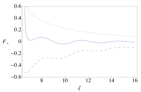
Figure 1: (Color online) Decay-rate correction function $F_{\perp}(\zeta)$ (with $\zeta=kr$) for cold scatterers and its constituents $F_{\mathrm{d},\perp}(\zeta)$ (        ) and $F_{\mathrm{r},\perp}(\zeta)$ (        ), for a spherical domain with dimensionless radius $kR=6$ containing cold absorbing spheres of dimensionless radius $ka=0.5$ and dielectric constant $\varepsilon=3.0+0.5i$.

Both $F_{\mathrm{c},\perp}$ and its constituent $F_{\mathrm{r},\perp}$ show a characteristic damped oscillating behavior, which is proportional to $\zeta^{-2}$ for large values of $\zeta$, in accordance with the asymptotic form given by (33) with (43). In contrast, the dielectric contribution $F_{\mathrm{d},\perp}$ is a monotonous function, which falls off like $\zeta^{-2}$ for large $\zeta$, as has been shown in (46). For atomic positions near the surface of the domain containing the scatterers the correction functions $F_{\mathrm{c},\perp}$ and $F_{\mathrm{d},\perp}$ diverge as $1/(\zeta-kR-ka)$, in accordance with (49), whereas $F_{\mathrm{r},\perp}$ stays finite.

The two contributions to $F_{\mathrm{c},\perp}$ are found to be mutually counteractive: $F_{\mathrm{d},\perp}$ is positive, whereas $F_{\mathrm{r},\perp}$ is negative. Their balance shifts when the dielectric medium becomes less absorptive, as is illustrated in Figs. 2,3.

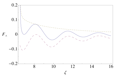
Figure 2: (Color online) Decay-rate correction function $F_{\perp}(\zeta)$ for cold scatterers and its constituents $F_{\mathrm{d},\perp}(\zeta)$ (        ) and $F_{\mathrm{r},\perp}(\zeta)$ (        ), for $kR=6$, $ka=0.5$ and $\varepsilon=3.0+0.1i$.

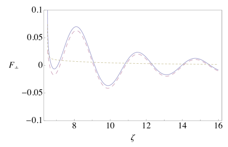
Figure 3: (Color online) Decay-rate correction function $F_{\perp}(\zeta)$ for cold scatterers and its constituents $F_{\mathrm{d},\perp}(\zeta)$ (        ) and $F_{\mathrm{r},\perp}(\zeta)$ (        ), for $kR=6$, $ka=0.5$ and $\varepsilon=3.0+0.01i$.

For hot scatterers the total decay-rate correction function $F_{\perp}$ is equal to the sum of $F_{\mathrm{r},\perp}$ and $[e^{\beta\hbar\omega}/(e^{\beta\hbar\omega}-1)]\,F_{\mathrm{d},\perp}$, according to (26). In Fig. 4 an example of the total correction function for hot scatterers is represented. Comparison with Fig. 1 shows how the balance between the dielectric and the radiative contributions gets shifted.

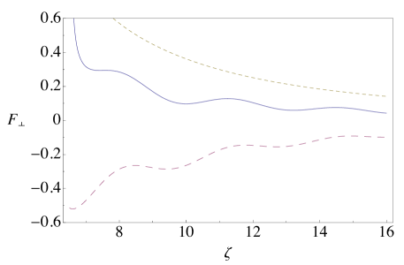
Figure 4: (Color online) Total decay-rate correction function $F_{\perp}(\zeta)$ for scatterers at finite temperature and its constituents $[e^{\beta\hbar\omega}/(e^{\beta\hbar\omega}-1)]\,F_{\mathrm{d},\perp}(\zeta)$ (        ) and $F_{\mathrm{r},\perp}(\zeta)$ (        ), for $kR=6$, $ka=0.5$, $\varepsilon=3.0+0.5i$ and $\beta\hbar\omega=1$.

The decay-rate correction function $F_{\parallel}$ for the longitudinal polarization direction largely behaves in a similar way, as can be seen in Figs. 5–6. However, in this case the oscillatory behavior for large distances shows a faster decay, with a damping proportional to $\zeta^{-4}$ in accordance with (28) and (41)–(42). The dielectric contribution $F_{\mathrm{d},\parallel}$ decays monotonously like $\zeta^{-4}$, as given in (44)–(45). The counterbalancing of the dielectric and radiative contributions occurs here as well, with a shifting balance as the absorptive power of the scatterers gets weaker. The inversely-linear divergent behavior for small distances, as given by (49), is clearly visible. In Fig. 6 it is shown how thermal radiation from the scatterers influences the longitudinal decay-rate correction function: both the total correction function and its dielectric part become larger owing to stimulated-emission effects, whereas the radiative part remains unchanged.

Figure 5: (Color online) Decay-rate correction function $F_{\parallel}(\zeta)$ for cold scatterers and its constituents $F_{\mathrm{d},\parallel}(\zeta)$ (        ) and $F_{\mathrm{r},\parallel}(\zeta)$ (        ), for $kR=6$, $ka=0.5$ and $\varepsilon=3.0+0.5i$.

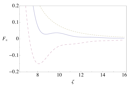
Figure 6: (Color online) Total decay-rate correction function $F_{\parallel}(\zeta)$ for scatterers at finite temperature and its constituents $[e^{\beta\hbar\omega}/(e^{\beta\hbar\omega}-1)]\,F_{\mathrm{d},\parallel}(\zeta)$ (        ) and $F_{\mathrm{r},\parallel}(\zeta)$ (        ), for $kR=6$, $ka=0.5$, $\varepsilon=3.0+0.5i$ and $\beta\hbar\omega=1$.

The present results for a spherical domain of radius $R$ filled with a dilute set of scatterers may be compared to those obtained from an effective-medium theory in which the domain contains a uniform dielectric with an effective dielectric constant $\varepsilon^{(\mathrm{eff})}$. For scatterers with a size much smaller than the wavelength one may use Maxwell Garnett theory MG04 , with the effective dielectric constant $\varepsilon^{(\mathrm{eff})}=1+3f(\varepsilon-1)/(\varepsilon+2)$. For a set of spherical scatterers with a radius $a$ that is not small compared to the wavelength (as in our model) the effective dielectric constant will depend on $ka$, as has been discussed in D89 ; R00 . It may be chosen as $\varepsilon^{(\mathrm{eff})}=1-3ifB^{e}_{1}/(k^{3}a^{3})$, with $B^{e}_{1}$ the electric-dipole scattering amplitude for a sphere with radius $a$ and dielectric constant $\varepsilon$, as given in (59). In the limit of small $ka$ the latter expression reduces to the Maxwell Garnett form.

The decay-rate correction functions that follow from the effective-medium theory will depend on the electric and magnetic multipole amplitudes $B^{p}_{l}(\varepsilon^{(\mathrm{eff})},R)$ (with $p=e,m$) for a uniform sphere with radius $R$ and dielectric constant $\varepsilon^{(\mathrm{eff})}$. Since the latter differs from 1 by a small amount, we may write the amplitudes $B^{p}_{l}(\varepsilon^{(\mathrm{eff})},R)$ as $(\varepsilon^{(\mathrm{eff})}-1)\bar{B}^{p}_{l}$, with reduced amplitudes $\bar{B}^{p}_{l}$ depending on $\rho=kR$:

$$\bar{B}^{e}_{l}=i^{l}\frac{2l+1}{l(l+1)}\rho\left\{(l+1+{\textstyle\frac{1}{2}}\rho^{2})[j_{l}(\rho)]^{2}+{\textstyle\frac{1}{2}}\rho^{2}[j_{l+1}(\rho)]^{2}\right.$$

$$\left.-(l+{\textstyle\frac{3}{2}})\rho j_{l}(\rho)j_{l+1}(\rho)\right\}\,,$$ (52)

$$\bar{B}^{m}_{l}=i^{l}\frac{2l+1}{l(l+1)}\rho\left\{{\textstyle\frac{1}{2}}\rho^{2}[j_{l}(\rho)]^{2}+{\textstyle\frac{1}{2}}\rho^{2}[j_{l+1}(\rho)]^{2}\right.$$

$$\left.-(l+{\textstyle\frac{1}{2}})\rho j_{l}(\rho)j_{l+1}(\rho)\right\}\,.$$ (53)

In terms of these reduced amplitudes the effective-medium decay-rate correction functions for cold scatterers become

$$F^{(\mathrm{eff})}_{\mathrm{c},\parallel}(r)=\frac{9}{2k^{3}a^{3}}\sum_{l=1}^{\infty}[l(l+1)]^{2}\mathrm{Re}\left[B^{e}_{1}(-i)^{l}\right.$$

$$\left.\times\bar{B}^{e}_{l}\frac{1}{k^{2}r^{2}}H_{l}(kr)\right]\,,$$ (54)

$$F^{(\mathrm{eff})}_{\mathrm{c},\perp}(r)=\frac{9}{4k^{3}a^{3}}\sum_{l=1}^{\infty}l(l+1)\mathrm{Re}\left\{B^{e}_{1}(-i)^{l}\right.$$

$$\left.\times\left[\bar{B}^{e}_{l}\frac{1}{k^{2}r^{2}}\bar{H}_{l}(kr)+\bar{B}^{m}_{l}H_{l}(kr)\right]\right\}\,.$$ (55)

The effective-medium dielectric decay-rate correction functions $F^{(\mathrm{eff})}_{\mathrm{d},p}(r)$ (with $p=\parallel,\perp$), which come into play for hot scatterers, have a similar form. They follow from (54)–(55) by replacing $H_{l}$ and $\bar{H}_{l}$ with the real functions $H_{\mathrm{d},l}$ and $\bar{H}_{\mathrm{d},l}$ (defined below (24)) and changing the overall sign. It should be noted that $(-i)^{l}\bar{B}^{q}_{l}$ (for $q=e,m$) is real, so that the functions $F^{(\mathrm{eff})}_{\mathrm{d},p}(r)$ are proportional to $\mathrm{Re}(B^{e}_{1})$.

Having established the expressions for the effective-medium decay-rate correction functions, we may compare the ensuing curves with those from our model in which the effects of inhomogeneities were taken into account. As an example, we shall consider the correction functions for the choice of parameters considered in Fig. 2.

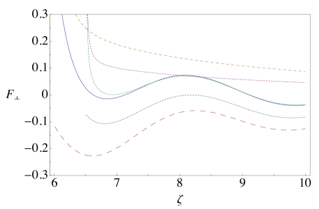
Figure 7: (Color online) Comparison of the decay-rate correction function $F^{(\mathrm{eff})}_{\perp}(\zeta)$ ( ) for a cold effective medium and its constituents $F^{(\mathrm{eff})}_{\mathrm{d},\perp}(\zeta)$ (        ), $F^{(\mathrm{eff})}_{\mathrm{r},\perp}(\zeta)$ (        ) with their scattering-medium counterparts $F_{\perp}(\zeta)$, $F_{\mathrm{d},\perp}(\zeta)$, $F_{\mathrm{r},\perp}(\zeta)$ (          ) for cold scatterers, as taken from Fig. 2, for $kR=6$, $ka=0.5$ and $\varepsilon=3.0+0.1i$.

From Fig. 7 it is clear that for large distances the effective-medium theory gives adequate results for the decay-rate correction function $F_{\perp}=F_{\mathrm{c},\perp}$ for cold scatterers, whereas it is off (by about a factor 2) for the dielectric part $F_{\mathrm{d},\perp}$ and also for the radiative part $F_{\mathrm{r},\perp}$, which play a role for hot scatterers. Thus, the effective-medium theory is not able to predict correct values for the decay-rate correction functions in the presence of hot scatterers. This state of affairs could have been expected from the general arguments put forward in R00 .

In the near zone the predictions of the effective-medium theory get even less reliable. As remarked at the end of Section IV, the small-distance asymptotic behavior of the decay-rate correction functions near a domain containing a set of discrete scatterers is different from that for a uniformly-filled domain. Moreover, the effective-medium theory misses the contribution of all higher-multipole scattering amplitudes, which get important near the scatterers. The resulting differences are clearly visible in the curves in Fig. 7.

Further insight in the cause of the discrepancies found in Fig. 7 is gained by determining the asymptotic behavior of the effective-medium decay-rate correction functions for large $kr$. Substituting the asymptotic form of the spherical Hankel functions contained in $H_{l}(kr)$ and $\bar{H}_{l}(kr)$ in (55), we get an expression for $F^{(\mathrm{eff})}_{\mathrm{c},\perp}(r)$ that is proportional to $\sum_{l=1}^{\infty}l(l+1)i^{l}(\bar{B}^{e}_{l}-\bar{B}^{m}_{l})$. Inserting (52)–(53), using the recurrence relations for $j_{l}$ NIST10 and employing the sum rule (103) we get the asymptotic result

$$F^{(\mathrm{eff})}_{\mathrm{c},\perp}(r)\simeq-\frac{9}{8k^{3}a^{3}}\left[\frac{1}{2}\sin(2\rho)-\rho\cos(2\rho)\right]\mathrm{Re}\left(B^{e}_{1}\frac{e^{2i\zeta}}{\zeta^{2}}\right)\,,$$ (56)

for large $\zeta=kr$. Comparison with (33) and (43) shows that we have recovered the contribution of the electric-dipole scattering amplitude. Clearly, it dominates the long-distance behavior of $F^{(\mathrm{eff})}_{\mathrm{c},\perp}(r)$, at least for the rather small dimensionless radius of the scatterers chosen here ($ka=0.5$).

The asymptotic form of $F^{(\mathrm{eff})}_{\mathrm{d},\perp}(r)$ may likewise be determined. It is found to be proportional to the sum $\sum_{l=1}^{\infty}l(l+1)(-i)^{l}(\bar{B}^{e}_{l}+\bar{B}^{m}_{l})$, which may be evaluated with the help of (100)–(102). One gets the asymptotic form for large $\zeta$:

$$F^{(\mathrm{eff})}_{\mathrm{d},\perp}(r)\simeq-\frac{3}{2k^{3}a^{3}}\frac{\rho^{3}}{\zeta^{2}}\mathrm{Re}(B^{e}_{1})\,.$$ (57)

Comparing with (38) and (46) we see that even the electric-dipole contributions differ: in the effective-medium theory the factor $C^{e}_{1}$ (defined in (78)) is replaced by $-\mathrm{Re}(B^{e}_{1})$. Since these differ by a factor 2.06 in the present case, the discrepancy in Fig. 7 is fully explained. Incidentally, it should be remarked that choosing a different form for the effective dielectric constant (for instance that of the original Maxwell Garnett theory) does not improve matters here. An analysis of the decay-rate correction functions for the longitudinal polarization ($\parallel$) and of their asymptotic behavior leads to similar conclusions.

VI Discussion

In the previous sections the modification of the decay rate of an excited atom in the vicinity of a spherical aggregate of randomly distributed small dielectric spheres at arbitrary temperature has been analyzed in detail. The changes could be described by a set of decay-rate correction functions that depend on three independent length scales, namely on the radii of both the scatterers and of the domain containing them, and on the distance between the atom and the center of the aggregate. Two types of decay-rate correction functions have been introduced, each for two different polarizations. The decay-rate correction functions $F_{\mathrm{c},\parallel}$ and $F_{\mathrm{c},\perp}$ describing the influence of cold scatterers were shown to exhibit a damped oscillatory behavior as a function of the atomic distance. In contrast, the dielectric correction functions $F_{\mathrm{d},\parallel}$ and $F_{\mathrm{d},\perp}$ that come into play for hot scatterers are monotonous as a function of the distance. The latter can be used as well to split the decay-rate correction functions for both cold and hot scatterers in contributions with a different origin, viz a dielectric and a radiative part. As we have seen, these two parts represent decay-modifying effects that may be counteracting, at least for sufficiently high absorptive power of the scatterers.

Two rather different representations for the decay-rate correction functions have been found in Sections III and IV. The first of these, which has been given in (19)-(20), follows by using addition theorems for vector spherical wave functions. The resulting expressions are triple sums over terms in which the electric and magnetic multipole contributions show up on an equal footing, while the three independent length scales are neatly separated. In the second representation, which involves sums of integrals over finite intervals, two of these length-scales (namely, the radius of the domain containing the scatterers and the distance of the atom to the center of the aggregate) get intertwined in the integrands and the boundaries of the integrals. Furthermore, the symmetry between the electric and magnetic contributions is no longer obvious. Nevertheless, this representation is quite useful, as it is more suitable for an efficient numerical evaluation of the decay-rate correction functions.

The changes in the decay rate that follow from (25) are proportional to the density $n_{s}$ of the scatterers. This is a direct consequence of the approximations for the Green function that were introduced in (11) and above (23). It amounts to the neglect of multiple-scattering events that would be important in an aggregate with a high filling fraction. When taking into account the effects of multiple scattering one expects a nonlinear dependence of the decay rate on the density. As an analytical evaluation is not feasible in that case, one has to resort to numerical simulations in order to treat dense aggregates of spheres.

A comparison of our results with those obtained from an effective-medium theory shows how the inhomogeneities brought about by the discrete scatterers affect the atomic decay rate. For scatterers that are far from the atom the dielectric correction functions $F_{\mathrm{d},p}$ and the radiative correction functions $F_{\mathrm{r},p}$ (for $p=\perp,\parallel$) both change considerably when the medium is smoothed, while their sums $F_{\mathrm{c},p}$ are almost left unchanged. Hence, for cold scatterers at large distances from the atom effective-medium theory is a useful approximation, whereas it is unreliable for scatterers at finite temperature. In contrast, for scatterers near the atom the predictions of effective-medium theory are inadequate at any temperature.

As we have seen, the rate of photon absorption of a ground-state atom near a collection of dielectric spheres emitting thermal radiation is determined by the same dielectric decay-rate correction functions $F_{\mathrm{d},\parallel}$ and $F_{\mathrm{d},\perp}$. If the atom is in a mixed state involving its ground state and excited state, both atomic decay and atomic absorption processes may occur, with rates given by (25) and (27). In that case a stationary situation may result with an atomic population ratio $n_{e}/n_{g}$ determined by the equilibrium condition $n_{e}\langle\Gamma_{\mathrm{t}}\rangle=n_{g}\langle\Gamma_{\mathrm{a}}\rangle$. Obviously, for positions far away from the aggregate the atom will end in its ground state, since the influence of the scatterers gets small. For distances near the surface of the domain containing the scatterers all correction functions become large and equal, apart from trivial factors 2. Hence, the vacuum decay rate $\Gamma_{0}$ in (25) can be neglected, so that $\langle\Gamma\rangle$ and $\langle\Gamma_{\mathrm{a}}\rangle$ are proportional in that case. As a consequence, the population ratio $n_{e}/n_{g}$ for an atom near the surface of the domain reduces to the standard Boltzmann factor $e^{-\beta\hbar\omega}$. Clearly, the aggregate of scatterers imposes its temperature on the atom in this case. For intermediate atomic positions the population ratio at which emission and absorption processes are in equilibrium differs from this simple result, since the influence of the scatterers gets smaller with distance. The precise form of the population ratio as a function of the atomic distance follows directly from the explicit expressions for the correction functions that have been determined in this paper.

Appendix A Green functions

The Green function in the presence of a dielectric sphere, with radius $a$ and complex dielectric constant $\varepsilon$, is the sum of the vacuum Green function $\textsf{{G}}_{0}$ and a scattering term $\textsf{{G}}_{\mathrm{s}}$. For a sphere centered at the origin the latter has the form T71 ; C95 ; LKLY94

$$\textsf{{G}}_{\mathrm{s}}(\mathbf{r},\mathbf{r}^{\prime},\omega+i0)=k\sum_{l=1}^{\infty}\sum_{m=-l}^{l}\frac{(-i)^{l}(-1)^{m}}{2l+1}$$

$$\times\left[B^{e}_{l}\,\mathbf{N}_{l,m}^{(h)}(\mathbf{r})\mathbf{N}_{l,-m}^{(h)}(\mathbf{r}^{\prime})+B^{m}_{l}\,\mathbf{M}_{l,m}^{(h)}(\mathbf{r})\mathbf{M}_{l,-m}^{(h)}(\mathbf{r}^{\prime})\right]$$

(58)

for $\mathbf{r}$ and $\mathbf{r}^{\prime}$ both outside the sphere.

The electric and magnetic multipole amplitudes read M08 ; BW99 ; SvW11

$$B^{p}_{l}=i^{l+1}\,\frac{2l+1}{l(l+1)}\,\frac{N^{p}_{l}}{D^{p}_{l}}\,,$$ (59)

with $l\geq 1$ and $p=e,m$. The numerators and denominators are given as

$$N^{e}_{l}=\varepsilon\,f_{l}(q)\,j_{l}(q^{\prime})-j_{l}(q)\,f_{l}(q^{\prime})\,,$$

$$N^{m}_{l}=f_{l}(q)\,j_{l}(q^{\prime})-j_{l}(q)\,f_{l}(q^{\prime})\,,$$

$$D^{e}_{l}=\varepsilon\,f^{(h)}_{l}(q)\,j_{l}(q^{\prime})-h^{(1)}_{l}(q)\,f_{l}(q^{\prime})\,,$$

$$D^{m}_{l}=f^{(h)}_{l}(q)\,j_{l}(q^{\prime})-h^{(1)}_{l}(q)\,f_{l}(q^{\prime})\,,$$ (60)

with $f_{l}(q)=(l+1)\,j_{l}(q)-q\,j_{l+1}(q)$ and $f^{(h)}_{l}(q)=(l+1)\,h^{(1)}_{l}(q)-q\,h^{(1)}_{l+1}(q)$. The spherical Bessel and Hankel functions depend on $q=ka$ and $q^{\prime}=\sqrt{\varepsilon}\,q$, with $a$ the radius of the sphere.

The vector spherical wave functions are defined as

$$\mathbf{M}_{l,m}(\mathbf{r})=\nabla\wedge[\mathbf{r}\psi_{l,m}(\mathbf{r})]\,,$$ (61)

$$\mathbf{N}_{l,m}(\mathbf{r})=k^{-1}\nabla\wedge[\nabla\wedge[\mathbf{r}\psi_{l,m}(\mathbf{r})]]\,,$$ (62)

where the scalar spherical wave function $\psi_{l,m}(\mathbf{r})$ stands for $j_{l}(kr)\,Y_{l,m}(\hat{\mathbf{r}})$, with $j_{l}$ a spherical Bessel function and $Y_{l,m}$ a spherical harmonic depending on the angles $(\theta,\varphi)$ that determine the direction of the unit vector $\hat{\mathbf{r}}=\mathbf{r}/r$. The superscripts $(h)$ in (58) denote the analogous vector spherical wave functions with spherical Hankel functions $h_{l}^{(1)}$ instead of $j_{l}$.

The vector spherical wave functions $\mathbf{M}_{l,m}(\mathbf{r})$ and $\mathbf{N}_{l,m}(\mathbf{r})$ satisfy addition theorems FJ87 ; C95 ; S61 ; C62 . To derive them in a concise way HC08 one may use an expansion for $\textsf{{I}}\,e^{i\mathbf{k}\cdot\mathbf{r}}$ that is a generalization of the standard Rayleigh expansion for $e^{i\mathbf{k}\cdot\mathbf{r}}$ in terms of spherical harmonics. The addition theorem for $\mathbf{M}_{l,m}(\mathbf{r})$ reads:

$$\mathbf{M}_{l,m}(\mathbf{r}^{\prime}+\mathbf{r}^{\prime\prime})=4\pi\sum_{l^{\prime}=1}^{\infty}\sum_{m^{\prime}=-l^{\prime}}^{l^{\prime}}\sum_{l^{\prime\prime}=0}^{\infty}\sum_{m^{\prime\prime}=-l^{\prime\prime}}^{l^{\prime\prime}}i^{l^{\prime}+l^{\prime\prime}-l}$$

$$\times\sqrt{\frac{l(l+1)}{l^{\prime}(l^{\prime}+1)}}\left[I^{(\mathrm{e})}_{l,m,l^{\prime},m^{\prime},l^{\prime\prime},m^{\prime\prime}}\mathbf{M}_{l^{\prime},m^{\prime}}(\mathbf{r}^{\prime})\right.$$

$$\left.+I^{(\mathrm{o})}_{l,m,l^{\prime},m^{\prime},l^{\prime\prime},m^{\prime\prime}}\mathbf{N}_{l^{\prime},m^{\prime}}(\mathbf{r}^{\prime})\right]\,\psi_{l^{\prime\prime},m^{\prime\prime}}(\mathbf{r^{\prime\prime}})\,.$$ (63)

The coefficients $I^{(\mathrm{p})}$ with $\mathrm{p}=\mathrm{e},\mathrm{o}$ are

$$I^{(\mathrm{p})}_{l,m,l^{\prime},m^{\prime},l^{\prime\prime},m^{\prime\prime}}=(-1)^{m+1}\sqrt{\frac{(2l+1)(2l^{\prime}+1)(2l^{\prime\prime}+1)}{4\pi}}$$

$$\times\left(\begin{array}[]{ccc}l&l^{\prime}&l^{\prime\prime}\\ m&-m^{\prime}&-m^{\prime\prime}\end{array}\right)\left(\begin{array}[]{ccc}l&l^{\prime}&l^{\prime\prime}\\ 1&-1&0\end{array}\right)\,\delta^{\mathrm{p}}_{l+l^{\prime}+l^{\prime\prime}}\,,$$ (68)

with symbols $\delta^{p}_{l}$ that have been defined below (17). The coefficients (68) agree with those given in TPM11 , and are equivalent with the results obtained in FJ87 and HC08 , as follows by employing a couple of identities for 6$j$-symbols TL96 .

The addition theorem for $\mathbf{N}_{l,m}$ has the same form as (63), with $\mathbf{M}$ and $\mathbf{N}$ interchanged. This follows immediately from the identities $\mathbf{M}_{l,m}=k^{-1}\nabla\wedge\mathbf{N}_{l,m}$ and $\mathbf{N}_{l,m}=k^{-1}\nabla\wedge\mathbf{M}_{l,m}$. Finally, we remark that analogous addition theorems hold true for $\mathbf{M}^{(h)}_{l,m}$ and $\mathbf{N}^{(h)}_{l,m}$. In particular, for $r^{\prime}\geq r^{\prime\prime}$ the addition theorem for $\mathbf{M}^{(h)}_{l,m}(\mathbf{r}^{\prime}+\mathbf{r}^{\prime\prime})$ follows from (63) by replacing both $\mathbf{M}$ and $\mathbf{N}$ by their counterparts $\mathbf{M}^{(h)}$ and $\mathbf{N}^{(h)}$.

For coinciding positions $\mathbf{r}$ and $\mathbf{r}^{\prime}$ the scattering term (58) in the Green function is diagonal in spherical coordinates:

$$\textsf{{G}}_{\mathrm{s}}(\mathbf{r},\mathbf{r},\omega+i0)=G_{\mathrm{s},\parallel}(r,\omega+i0)\mathbf{e}_{r}\mathbf{e}_{r}$$

$$+G_{\mathrm{s},\perp}(r,\omega+i0)(\mathbf{e}_{\theta}\mathbf{e}_{\theta}+\mathbf{e}_{\varphi}\mathbf{e}_{\varphi})\,,$$ (69)

with components given in DKW01 ; SvW11 .

If $\mathbf{r}^{\prime}$ is situated inside the sphere and $\mathbf{r}$ is outside, the full Green function $\textsf{{G}}_{0}+\textsf{{G}}_{\mathrm{s}}\equiv\textsf{{G}}_{0\mathrm{s}}$ reads T71 ; C95 ; LKLY94

$$\textsf{{G}}_{0\mathrm{s}}(\mathbf{r},\mathbf{r}^{\prime},\omega+i0)=\frac{1}{a}\sum_{l=1}^{\infty}\sum_{m=-l}^{l}\frac{(-i)^{l+1}(-1)^{m}}{2l+1}$$

$$\times\left[A^{e}_{l}\,\mathbf{N}_{l,m}^{(h)}(\mathbf{r})\mathbf{N}_{l,-m}^{(\varepsilon)}(\mathbf{r}^{\prime})+A^{m}_{l}\,\mathbf{M}_{l,m}^{(h)}(\mathbf{r})\mathbf{M}_{l,-m}^{(\varepsilon)}(\mathbf{r}^{\prime})\right]\,.$$

(70)

The modified vector spherical wave functions $\mathbf{M}_{l,m}^{(\varepsilon)}$ and $\mathbf{N}_{l,m}^{(\varepsilon)}$ follow from (61) and (62) upon replacing $k$ by $k^{\prime}=\sqrt{\varepsilon}k$. Furthermore, the amplitudes $A_{l}^{p}$ are defined as

$$A_{l}^{p}=i^{l+1}\,\frac{2l+1}{l(l+1)}\,\frac{c_{p}}{D^{p}_{l}}\,,$$ (71)

with $l\geq 1$ and $p=e,m$. The coefficients in the numerator are $c_{e}=\sqrt{\epsilon}$, $c_{m}=1$, while the denominators follow from (60).

In the main text we need expressions for integrals over scalar products of the modified vector spherical wave functions. These can be evaluated by starting from (61)-(62), employing the standard expressions for the curl of a vector in spherical coordinates and evaluating the angular integrals. In this way one gets:

$$\int_{r<a}d\mathbf{r}\,\mathbf{M}_{l,m}^{(\varepsilon)}(\mathbf{r})\cdot\mathbf{M}_{l^{\prime},m^{\prime}}^{(\varepsilon)\ast}(\mathbf{r})=\delta_{l,l^{\prime}}\delta_{m,m^{\prime}}l(l+1)I_{l}^{(\varepsilon)}(a)\,,$$

(72)

$$\int_{r<a}d\mathbf{r}\,\mathbf{N}_{l,m}^{(\varepsilon)}(\mathbf{r})\cdot\mathbf{N}_{l^{\prime},m^{\prime}}^{(\varepsilon)\ast}(\mathbf{r})=\delta_{l,l^{\prime}}\delta_{m,m^{\prime}}\frac{l(l+1)}{2l+1}$$

$$\times\left[(l+1)I_{l-1}^{(\varepsilon)}(a)+lI_{l+1}^{(\varepsilon)}(a)\right]\,,$$ (73)

$$\int_{r<a}d\mathbf{r}\,\mathbf{M}_{l,m}^{(\varepsilon)}(\mathbf{r})\cdot\mathbf{N}_{l^{\prime},m^{\prime}}^{(\varepsilon)\ast}(\mathbf{r})=0\,,$$ (74)

with the radial integrals $I_{l}^{(\varepsilon)}(a)=\int_{0}^{a}dr\,r^{2}|j_{l}(k^{\prime}r)|^{2}$. The latter are given as:

$$I_{l}^{(\varepsilon)}(a)=2a^{2}\mathrm{Re}\left[\frac{k^{\prime}}{k^{\prime 2}-(k^{\prime\ast})^{2}}j_{l+1}(k^{\prime}a)j_{l}(k^{\prime\ast}a)\right]\,,$$ (75)

as may be verified by differentiation. This identity is useful in proving relations between $A_{l}^{p}$ and $B^{p}_{l}$. In fact, by using the Wronskian for spherical Bessel functions NIST10 one may derive the following equalities for $l\geq 1$:

$$\left[\mathrm{Im}\,\varepsilon(\omega+i0)\right]\,I_{l}^{(\varepsilon)}(a)|A^{m}_{l}|^{2}=\frac{2l+1}{l(l+1)}\frac{a^{2}}{k}C_{l}^{m}\,,$$ (76)

$$\left[\mathrm{Im}\,\varepsilon(\omega+i0)\right]\left[(l+1)I_{l-1}^{(\varepsilon)}(a)+lI_{l+1}^{(\varepsilon)}(a)\right]|A^{e}_{l}|^{2}=$$

$$=\frac{(2l+1)^{2}}{l(l+1)}\frac{a^{2}}{k}C_{l}^{e}\,.$$ (77)

Here we introduced the abbreviations

$$C_{l}^{p}=\mathrm{Re}\left[(-i)^{l+1}B^{p}_{l}\right]-\frac{l(l+1)}{2l+1}|B^{p}_{l}|^{2}\,,$$ (78)

for $p=e,m$ and $l\geq 1$.

Appendix B Evaluation of integrals

In the main text we introduced the indefinite integrals

$$I_{l_{1},l_{2},n}(z)=\int^{z}du\,u^{-n}h^{(1)}_{l_{1}}(u)\,h^{(1)}_{l_{2}}(u)\,,$$ (79)

for real $z>0$, integer $n$ and non-negative integers $l_{1},l_{2}$. We need information about these integrals for the diagonal case with $l_{1}=l_{2}=l$ and for the off-diagonal case with $l_{1}=l_{2}-1=l$. In the following we shall omit any additive constants which may show up when deriving expressions for these integrals.

The diagonal integrals with $l_{1}=l_{2}=l$ satisfy a recursion relation of the form

$$(2l+n+3)I_{l+1,l+1,n}(z)=(2l-n+1)I_{l,l,n}(z)$$

$$-z^{-n+1}\left\{\left[h^{(1)}_{l}(z)\right]^{2}+\left[h^{(1)}_{l+1}(z)\right]^{2}\right\}\,,$$ (80)

as may be verified by differentiation. When these diagonal integrals are known, the non-diagonal integrals follow from the relation

$$I_{l,l+1,n}(z)={\textstyle\frac{1}{2}}(2l-n)I_{l,l,n+1}(z)-{\textstyle\frac{1}{2}}z^{-n}\left[h^{(1)}_{l}(z)\right]^{2},$$ (81)

which likewise may be established by differentiation.

The recursion relation (80) can be employed to link $I_{l,l,n}(z)$ to a lower-order integral $I_{l_{0},l_{0},n}(z)$, with $l_{0}<l$. When $n$ is even, we may choose $l_{0}=0$. For odd $n\leq-3$ the recursion stops at a positive value of $l$. As a consequence, one should choose $l_{0}=-{\textstyle\frac{1}{2}}n-{\textstyle\frac{1}{2}}>0$ in that case. With these values of $l_{0}$ the solution of the recursion relation reads for $l>l_{0}$:

$$I_{l,l,n}(z)=\frac{(l_{0}-{\textstyle\frac{1}{2}}n+{\textstyle\frac{1}{2}})_{l-l_{0}}}{(l_{0}+{\textstyle\frac{1}{2}}n+{\textstyle\frac{3}{2}})_{l-l_{0}}}I_{l_{0},l_{0},n}(z)$$

$$-\frac{1}{2}z^{-n+1}\sum^{l-1}_{k=l_{0}+1}(2k+1)\frac{(k-{\textstyle\frac{1}{2}}n+{\textstyle\frac{3}{2}})_{l-k-1}}{(k+{\textstyle\frac{1}{2}}n+{\textstyle\frac{1}{2}})_{l-k+1}}[h_{k}^{(1)}(z)]^{2}$$

$$-\frac{1}{2}z^{-n+1}\frac{(l_{0}-{\textstyle\frac{1}{2}}n+{\textstyle\frac{3}{2}})_{l-l_{0}-1}}{(l_{0}+{\textstyle\frac{1}{2}}n+{\textstyle\frac{3}{2}})_{l-l_{0}}}[h_{l_{0}}^{(1)}(z)]^{2}$$

$$-z^{-n+1}\frac{1}{2l+n+1}[h^{(1)}_{l}(z)]^{2}\,,$$ (82)

with Pochhammer symbols $(a)_{n}=a(a+1)\cdots(a+n-1)$. For $l=l_{0}+1$ the sum drops out. As we shall see below, the sum can be evaluated in closed form for all even $n\leq-2$ and for all odd $n\geq 1$. We shall consider in the following the diagonal integrals with even $n=0,-2$ and with odd $n=3,1,-1,-3,-5$, as these are needed in the main text.

For $n=0$ the expression (82) becomes, upon choosing $l_{0}=0$ and evaluating the initial condition in terms of the exponential integral as $I_{0,0,0}(z)=2iE_{1}(-2iz)+e^{2iz}/z$:

$$I_{l,l,0}(z)=-\frac{2z}{2l+1}\sum_{k=0}^{l}[h^{(1)}_{k}(z)]^{2}+\frac{z}{2l+1}[h^{(1)}_{l}(z)]^{2}$$

$$+\frac{2i}{2l+1}E_{1}(-2iz)\,,$$ (83)

for all $l\geq 0$. The exponential integral can be rewritten NIST10 in terms of sine and cosine integrals as $E_{1}(-2iz)=-\mathrm{Ci}(2z)-i\mathrm{Si}(2z)+i\pi/2$.

For $n=-2$ one gets, again taking $l_{0}=0$ and inserting the (trivial) result for $I_{0,0,-2}$:

$$I_{l,l,-2}(z)=-2(2l+1)z^{3}\sum_{k=0}^{l}\frac{1}{(2k-1)(2k+3)}[h^{(1)}_{k}(z)]^{2}$$

$$+\frac{z^{3}}{2l+3}[h^{(1)}_{l}(z)]^{2}+\frac{1}{2}(2l+1)(2z+i)e^{2iz}\,.$$ (84)

The sum at the right-hand side can be evaluated with the help of (94). In that way we arrive at the simpler result

$$I_{l,l,-2}(z)=\frac{1}{2}z^{3}[h^{(1)}_{l}(z)]^{2}+\frac{1}{2}z^{3}[h^{(1)}_{l+1}(z)]^{2}$$

$$-\frac{1}{2}(2l+1)z^{2}h^{(1)}_{l}(z)h^{(1)}_{l+1}(z)\,,$$ (85)

for $l\geq 0$.

Next we consider the diagonal integrals with odd values of $n$. For $n=3$ we choose $l_{0}=0$ in (82). For $l\geq 2$ the first and third terms at the right-hand side drop out. As a result we get:

$$I_{l,l,3}(z)=-\frac{1}{2(l-1)_{4}z^{2}}\sum_{k=1}^{l}(2k+1)k(k+1)[h^{(1)}_{k}(z)]^{2}$$

$$+\frac{1}{2(l-1)z^{2}}[h^{(1)}_{l}(z)]^{2}\,,$$ (86)

for $l\geq 2$. As before, the sum at the right-hand side can be evaluated in explicit form in terms of $h^{(1)}_{l}$ and $h^{(1)}_{l+1}$, as is shown in Appendix C. Upon substituting (97) for $p=1$ we arrive at the expression:

$$\!\!\!\!\!\!I_{l,l,3}(z)=\left[\frac{z^{2}}{3(l-1)_{4}}+\frac{1}{6(l-1)l}+\frac{1}{2(l-1)z^{2}}\right][h^{(1)}_{l}(z)]^{2}$$

$$+\left[\frac{z^{2}}{3(l-1)_{4}}+\frac{1}{6(l-1)(l+2)}\right][h^{(1)}_{l+1}(z)]^{2}$$

$$-\left[\frac{2z}{3(l-1)l(l+2)}+\frac{1}{3(l-1)z}\right]h^{(1)}_{l}(z)h^{(1)}_{l+1}(z)\,,$$ (87)

for $l\geq 2$. This result is useless for $l=0,1$. These special cases can be evaluated in terms of the exponential integral, as in (83).

For $n=1$ (and $l_{0}=0$) the first term at the right-hand side of (82) drops out for all $l\geq 1$. The special case $l=0$, which leads to an exponential integral, has to be treated separately. For $l\geq 1$ one gets an expression involving a sum that can be evaluated with the help of the sum rule (96). The final result is

$$I_{l,l,1}(z)=\left[\frac{z^{2}}{2l(l+1)}+\frac{1}{2l}\right][h^{(1)}_{l}(z)]^{2}$$

$$+\frac{z^{2}}{2l(l+1)}[h^{(1)}_{l+1}(z)]^{2}-\frac{z}{l}h^{(1)}_{l}(z)h^{(1)}_{l+1}(z)\,,$$ (88)

for $l\geq 1$.

For $n=-1$ we get from (82) (for $l_{0}=0$) upon inserting the initial condition $I_{0,0,-1}(z)=E_{1}(-2iz)$:

$$I_{l,l,-1}(z)=-\frac{1}{2}z^{2}\sum_{k=1}^{l}\frac{2k+1}{k(k+1)}[h^{(1)}_{k}(z)]^{2}$$

$$+\frac{z^{2}}{2(l+1)}[h^{(1)}_{l}(z)]^{2}+E_{1}(-2iz)+\frac{1}{2}e^{2iz}\,,$$ (89)

for all $l\geq 0$. As it turns out, the sum cannot be simplified with the help of one of the sum rules in Appendix C.

When considering the case $n=-3$ in (82) we have to choose $l_{0}=1$ and substitute the initial condition for $l=1$ that follows by a direct evaluation as $I_{1,1,-3}(z)=E_{1}(-2iz)+(-{\textstyle\frac{1}{2}}iz+{\textstyle\frac{5}{4}})e^{2iz}$. The ensuing expression for $I_{l,l,-3}(z)$ contains a sum over squares of spherical Hankel functions $h^{(1)}_{k}(z)$, with a coefficient $(2k+1)/{(k-1)_{4}}$. This sum may be rewritten with the help of the identity (98) for $p=1$. As a result we get for all $l\geq 0$:

$$I_{l,l,-3}(z)=-\frac{1}{4}l(l+1)z^{2}\sum_{k=1}^{l}\frac{2k+1}{k(k+1)}[h^{(1)}_{k}(z)]^{2}$$

$$+\frac{1}{4}z^{4}[h^{(1)}_{l}(z)]^{2}+\frac{1}{4}z^{4}[h^{(1)}_{l+1}(z)]^{2}$$

$$-\frac{1}{2}lz^{3}h^{(1)}_{l}(z)h^{(1)}_{l+1}(z)+\frac{1}{2}l(l+1)E_{1}(-2iz)$$

$$+\frac{1}{4}l(l+1)e^{2iz}\,,$$ (90)

which contains the same sum as (89).

The last diagonal integral that we have to evaluate is the case with $n=-5$. It follows from (82) by choosing $l_{0}=2$ and inserting the initial condition for $l=2$, which has to be calculated by hand as $I_{2,2,-5}(z)=9E_{1}(-2iz)+({\textstyle\frac{1}{2}}iz^{3}-{\textstyle\frac{15}{4}}z^{2}-{\textstyle\frac{45}{4}}iz+{\textstyle\frac{117}{8}})e^{2iz}$. One encounters a sum over squares of spherical Hankel functions with a coefficient containing $(k-2)_{6}$ in the denominator. Again (98) (for $p=1,2$) is helpful in reducing this sum, so that we arrive at the expression:

$$I_{l,l,-5}(z)=-\frac{3}{16}(l-1)_{4}\,z^{2}\sum_{k=1}^{l}\frac{2k+1}{k(k+1)}[h^{(1)}_{k}(z)]^{2}$$

$$+\left[\frac{3}{16}l(l-1)+\frac{1}{8}z^{2}\right]z^{4}[h^{(1)}_{l}(z)]^{2}$$

$$+\left[\frac{3}{16}(l-1)(l+2)+\frac{1}{8}z^{2}\right]z^{4}[h^{(1)}_{l+1}(z)]^{2}$$

$$-\left[\frac{3}{8}l(l+2)+\frac{1}{4}z^{2}\right](l-1)z^{3}h^{(1)}_{l}(z)h^{(1)}_{l+1}(z)$$

$$+\frac{3}{8}(l-1)_{4}\,E_{1}(-2iz)+\frac{3}{16}(l-1)_{4}e^{2iz}\,,$$ (91)

for all $l\geq 0$. The same sum as in (89) appears once again.

The off-diagonal integrals $I_{l,l+1,n}(z)$ with $n=-4,-2,-1,0,2$ follow from the above diagonal integrals by employing (81).

To evaluate the dielectric decay-rate correction functions $F_{\mathrm{d},\parallel}$ and $F_{\mathrm{d},\perp}$ we also need information about indefinite integrals with spherical Hankel functions and their complex conjugates in the integrand:

$$I^{\prime}_{l_{1},l_{2},n}(z)=\int^{z}du\,u^{-n}h^{(1)}_{l_{1}}(u)\,[h^{(1)}_{l_{2}}(u)]^{\ast}\,,$$ (92)

for $z>0$, integer $n$ and non-negative integers $l_{1},l_{2}$. Explicit expressions for these integrals can be derived in a similar way as above. The results are analogous, with some subtle differences. For $n=0$ and $l_{1}=l_{2}=l$ for instance, one finds on a par with (83) for all $l\geq 0$:

$$I^{\prime}_{l,l,0}(z)=-\frac{2z}{2l+1}\sum_{k=0}^{l}|h^{(1)}_{k}(z)|^{2}+\frac{z}{2l+1}|h^{(1)}_{l}(z)|^{2}\,.$$ (93)

The term with the exponential integral is missing here, while the squares of the spherical Hankel functions are replaced by the squares of their moduli. We refrain from listing here the expressions for the other $I^{\prime}_{l_{1},l_{2},n}$ that are needed in the evaluation of $F_{\mathrm{d},\parallel}$ and $F_{\mathrm{d},\perp}$.

Appendix C Sums of squares of spherical Hankel functions

In Appendix B sums of squares of spherical Hankel functions show up. Some of these may be evaluated as simple combinations of $h^{(1)}_{l}$ and $h^{(1)}_{l+1}$. An example is the sum occurring in (84). By induction with respect to $l$ one proves the following sum rule for $l\geq 0$:

$$\sum^{l}_{k=0}\frac{1}{(2k-1)(2k+3)}[h^{(1)}_{k}]^{2}=-\frac{1}{4(2l+3)}[h^{(1)}_{l}]^{2}$$

$$-\frac{1}{4(2l+1)}[h^{(1)}_{l+1}]^{2}+\frac{1}{4z}h^{(1)}_{l}h^{(1)}_{l+1}$$

$$+\left(\frac{1}{2z^{2}}+\frac{i}{4z^{3}}\right)e^{2iz}\,,$$ (94)

where we omitted the argument $z$ of the spherical Hankel functions. It turns out that this sum rule is the first in a hierarchy of sum rules with an increasing number of factors in the denominator of the coefficient in the summand. In fact, one may prove for all $p\geq 0$ and all $l\geq 0$:

$$\sum_{k=0}^{l}\frac{2k+1}{(k-p-{\textstyle\frac{1}{2}})_{2p+3}}[h^{(1)}_{k}]^{2}=$$

$$\!\!\!\!\!\!\!\!=-\frac{1}{2}\left[\sum_{k=0}^{p}\frac{(p-k+1)_{k}}{(p-k+\frac{1}{2})_{k+1}(l-p+k+\frac{3}{2})_{2p-2k+1}}\frac{1}{z^{2k}}\right][h^{(1)}_{l}]^{2}$$

$$\!\!\!\!\!\!\!\!-\frac{1}{2}\left[\sum_{k=0}^{p}\frac{(p-k+1)_{k}}{(p-k+\frac{1}{2})_{k+1}(l-p+k+\frac{1}{2})_{2p-2k+1}}\frac{1}{z^{2k}}\right][h^{(1)}_{l+1}]^{2}$$

$$\!\!\!\!\!\!\!\!+\left[\sum_{k=0}^{p}\frac{(p-k+1)_{k}}{(p-k+\frac{1}{2})_{k+1}(l-p+k+\frac{3}{2})_{2p-2k}}\frac{1}{z^{2k+1}}\right]h^{(1)}_{l}h^{(1)}_{l+1}$$

$$+R_{1,p}(z)\,.$$ (95)

The last term, which is independent of $l$, follows by taking $l=0$ on both sides of the identity. For small values of $p$ the polynomials in $1/z$ are of low degree, so that this identity yields an efficient way of evaluating the sum, in particular for higher $l$.

A second hierarchy of sum rules, with an increasing number of factors in the numerator of the summand, can be established as well. The first sum rule in this hierarchy reads

$$\sum_{k=0}^{l}(2k+1)[h^{(1)}_{k}]^{2}=$$

$$=-z^{2}[h^{(1)}_{l}]^{2}-z^{2}[h^{(1)}_{l+1}]^{2}+2(l+1)zh^{(1)}_{l}h^{(1)}_{l+1}\,,$$ (96)

for $l\geq 0$. The complete hierarchy reads for all $p\geq 0$ and $l\geq p$:

$$\sum_{k=p}^{l}(2k+1)(k-p+1)_{2p}[h^{(1)}_{k}]^{2}=$$

$$\!\!\!\!\!\!\!\!=-\frac{1}{2}\left[\sum_{k=0}^{p}\frac{(p-k+1)_{k}(l-p+k+2)_{2p-2k}}{(p-k+\frac{1}{2})_{k+1}}z^{2k+2}\right][h^{(1)}_{l}]^{2}$$

$$\!\!\!\!\!\!\!\!-\frac{1}{2}\left[\sum_{k=0}^{p}\frac{(p-k+1)_{k}(l-p+k+1)_{2p-2k}}{(p-k+\frac{1}{2})_{k+1}}z^{2k+2}\right][h^{(1)}_{l+1}]^{2}$$

$$\!\!\!\!\!\!\!\!+\left[\sum_{k=0}^{p}\frac{(p-k+1)_{k}(l-p+k+1)_{2p-2k+1}}{(p-k+\frac{1}{2})_{k+1}}z^{2k+1}\right]h^{(1)}_{l}h^{(1)}_{l+1}\,.$$

(97)

A remainder function independent of $l$ does not occur here.

Apart from these sum rules one may prove several hierarchies of identities relating sums of a similar type as above. A first one of these reads as follows

$$\!\!\!\!\!\!\!\!z^{2}\sum_{k=p+1}^{l}\frac{2k+1}{(k-p)_{2p+2}}[h^{(1)}_{k}]^{2}=\frac{2p-1}{2p}\sum_{k=p}^{l}\frac{2k+1}{(k-p+1)_{2p}}[h^{(1)}_{k}]^{2}$$

$$-\frac{1}{2p(l-p+2)_{2p}}z^{2}[h^{(1)}_{l}]^{2}-\frac{1}{2p(l-p+1)_{2p}}z^{2}[h^{(1)}_{l+1}]^{2}$$

$$+\frac{1}{p(l-p+2)_{2p-1}}zh^{(1)}_{l}h^{(1)}_{l+1}+R_{2,p}(z)\,,$$ (98)

for $p\geq 1$ and $l\geq p$. The remainder function $R_{2,p}(z)$ follows by putting $l=p$, and discarding the left-hand side. In Appendix B this identity has been employed for $p=1$ and $p=2$, in order to reduce several sums over squares of spherical Hankel functions with complicated coefficients to sums with simpler coefficients.

Yet another hierarchy of identities relates sums with coefficients containing an increasing number of factors in the numerator:

$$\sum_{k=0}^{l}(2k+1)(k-p+{\textstyle\frac{1}{2}})_{2p+1}[h^{(1)}_{k}]^{2}=$$

$$=\frac{2p+1}{2(p+1)}z^{2}\sum_{k=0}^{l}(2k+1)(k-p+{\textstyle\frac{3}{2}})_{2p-1}[h^{(1)}_{k}]^{2}$$

$$-\frac{(l-p+\frac{3}{2})_{2p+1}}{2(p+1)}z^{2}[h^{(1)}_{l}]^{2}-\frac{(l-p+\frac{1}{2})_{2p+1}}{2(p+1)}z^{2}[h^{(1)}_{l+1}]^{2}$$

$$+\frac{(l-p+\frac{1}{2})_{2p+2}}{p+1}zh^{(1)}_{l}h^{(1)}_{l+1}+R_{3,p}(z)\,,$$ (99)

for $p\geq 0$ and $l\geq 0$. For $p=0$ the Pochhammer symbol $(k+\frac{3}{2})_{-1}$ in the sum at the right-hand side should be read as $1/(k+\frac{1}{2})$, as follows by using the alternative form $(a)_{n}=\Gamma(a+n)/\Gamma(a)$ NIST10 . The remainder function $R_{3,p}(z)$ is independent of $l$ and follows by taking $l=0$.

Similar sum rules may be established for sums over squares of the modulus $|h^{(1)}_{l}(z)|$ of a spherical Hankel function (with a real argument $z$), or, even more generally, for sums over products $f_{l}(z)g_{l}(z)$, with $f_{l}$ and $g_{l}$ equal to $j_{l}$, $y_{l}$, $h_{l}^{(1)}$ or $h_{l}^{(2)}$, independently. For instance, one may prove a sum rule like (95), with all $[h^{(1)}_{k}]^{2}$ replaced by $|h^{(1)}_{k}|^{2}$ and the product $h^{(1)}_{l}h^{(1)}_{l+1}$ replaced by its real part ${\textstyle\frac{1}{2}}[h^{(1)}_{l}h^{(2)}_{l+1}+h^{(1)}_{l+1}h^{(2)}_{l}]$ (for real arguments). The remainder function is found to be 0 in that case. The analogues of the sum rules (95), (97) and (98) for the modulus of the spherical Hankel functions are useful in deriving suitable expressions for the integrals $I^{\prime}_{l_{1},l_{2},n}$ in Appendix B.

The above sum rules, with squares $[j_{k}(z)]^{2}$ instead of $[h^{(1)}_{k}(z)]^{2}$, may be employed to derive identities for infinite sums that have been used in Section V. The analogue of (97) for spherical Bessel functions contains a remainder function $p!z^{2p}/({\textstyle\frac{3}{2}})_{p}$. Upon taking the limit $l\rightarrow\infty$, the other terms at the right-hand side drop out, so that one is left with the equality

$$\sum_{k=p}^{\infty}(2k+1)(k-p+1)_{2p}[j_{k}(z)]^{2}=\frac{p!}{({\textstyle\frac{3}{2}})_{p}}z^{2p}\,,$$ (100)

for $p\geq 0$. For $p=0$ this sum rule is well-known NIST10 , while for general $p\geq 0$ it agrees with an identity in L69 . Likewise, the analogue of (99) for $[j_{k}(z)]^{2}$ contains the remainder function $-(-p-{\textstyle\frac{1}{2}})_{2p+1}[\cos(2z)+(p+{\textstyle\frac{1}{2}})\sin(2z)/z]/(2(p+1))$. In the limit of infinite $l$ the second, third and fourth terms at the right-hand side drop out, so that a simple recursion relation connecting infinite sums is obtained. It may be combined with the initial condition NIST10

$$\sum_{k=0}^{\infty}[j_{k}(z)]^{2}=\frac{\mathrm{Si}(2z)}{2z}$$ (101)

to derive expressions for all sums of the form $\sum_{k=0}^{\infty}(2k+1)(k-p+{\textstyle\frac{1}{2}})_{2p+1}[j_{k}(z)]^{2}$ with $p\geq 0$. In particular, one gets for $p=0$:

$$\sum_{k=0}^{\infty}(2k+1)^{2}[j_{k}(z)]^{2}=z\mathrm{Si}(2z)+\frac{\sin(2z)}{4z}+\frac{1}{2}\cos(2z)\,,$$ (102)

which is consistent with an identity involving the generalized hypergeometric function $\mbox{}_{1}F_{2}({\textstyle\frac{1}{2}};{\textstyle\frac{5}{2}},{\textstyle\frac{5}{2}};-z^{2})$ in L69 . Finally, an infinite sum rule with alternating signs:

$$\sum_{k=p}^{\infty}(-1)^{k}(2k+1)(k-p+1)_{2p}[j_{k}(z)]^{2}=(-1)^{p}p!z^{p}j_{p}(2z)$$ (103)

has been employed in Section V for $p=0,1$. For $p=0$ it is well-known NIST10 , whereas for general $p\geq 0$ it can be found in L69 .

References

• (1) E.M. Purcell, Phys. Rev. 69, 681 (1946).
• (2) K.H. Drexhage, J. Lumin. 1,2, 693 (1970).
• (3) R.R. Chance, A. Prock and R. Silbey, J. Chem. Phys. 60, 2744 (1974).
• (4) G.S. Agarwal, Phys. Rev. A 12, 1475 (1975).
• (5) M.S. Yeung and T.K. Gustafson, Phys. Rev. A 54, 5227 (1996).
• (6) S. Scheel, L. Knöll and D.-G. Welsch, Acta Phys. Slov. 49, 585 (1999).
• (7) C. Eberlein and R. Zietal, Phys. Rev. A 86, 022111 (2012).
• (8) R. Ruppin, J. Chem. Phys. 76, 1681 (1982).
• (9) G.S. Agarwal and S.V. ONeil, Phys. Rev. B 28, 487 (1983).
• (10) Y.S. Kim, P.T. Leung and T.F. George, Surf. Sci. 195, 1 (1988).
• (11) H.T. Dung, L. Knöll, and D.-G. Welsch, Phys. Rev. A 62, 053804 (2000).
• (12) H.T. Dung, L. Knöll, and D.-G. Welsch, Phys. Rev. A 64, 013804 (2001).
• (13) V.V. Klimov and V.S. Letokhov, Laser Phys. 15, 61 (2005).
• (14) H.Y. Chung, P.T. Leung and D.P. Tsai, J. Chem. Phys. 136, 184106 (2012).
• (15) H.Y. Chung, P.T. Leung and D.P. Tsai, Phys. Rev. B 86, 155413 (2012).
• (16) V.V. Klimov, M. Ducloy, and V.S. Letokhov, Quantum Electron. 31, 569 (2001).
• (17) V. Yannopapas and N.V. Vitanov, Phys. Rev. B 75, 115124 (2007).
• (18) V. Yannopapas and N.V. Vitanov, J. Phys. Condensed Matter 19, 096210 (2007).
• (19) L.S. Froufe-Pérez, R. Carminati and J.J. Sáenz, Phys. Rev. A 76, 013835 (2007).
• (20) R. Pierrat and R. Carminati, Phys. Rev. A 81, 063802 (2010).
• (21) L.G. Suttorp and A.J. van Wonderen, Opt. Commun. 284, 2943 (2011).
• (22) A.V. Shchegrov, K. Joulain, R. Carminati and J.-J. Greffet, Phys. Rev. Lett. 85, 1548 (2000).
• (23) K. Joulain, J.-Ph. Mulet, F. Marquier, R. Carminati and J.-J. Greffet, Surf. Sci. Rep. 57, 59 (2005).
• (24) B. Huttner and S.M. Barnett, Phys. Rev. A 46, 4306 (1992).
• (25) L.G. Suttorp and A.J. van Wonderen, Europhys. Lett. 67, 766 (2004).
• (26) L.G. Suttorp and A.J. van Wonderen, J. Phys. B 43, 105501 (2010).
• (27) K. Henneberger and F. Richter, Phys. Rev. A 80, 013807 (2009).
• (28) S. Savasta, O. Di Stefano, and R.  Girlanda, Phys. Rev. A 65, 043801 (2002).
• (29) L. Tsang, J.A. Kong and R.T. Shin, Theory of Microwave Remote Sensing (Wiley, New York, 1985), Chapters 5, 6.
• (30) L. Tsang and J.A. Kong, Scattering of Electromagnetic Waves: Advanced Topics (Wiley, New York, 2001), Chapter 5.
• (31) NIST Handbook of Mathematical Functions, edited by F.W.J. Olver, D.W. Lozier et al (Cambridge University Press, Cambridge, 2010).
• (32) B.U. Felderhof and R.B. Jones, J. Math. Phys. 28, 836 (1987).
• (33) J.C. Maxwell Garnett, Phil. Trans. Roy. Soc.A 203 385 (1904).
• (34) W.T. Doyle, Phys. Rev. B 39 9852 (1989).
• (35) R. Ruppin, Opt. Commun. 182 273 (2000).
• (36) C.-T. Tai, Dyadic Green’s functions in Electromagnetic Theory (Intext Publ., New York, 1971).
• (37) W.C. Chew, Waves and Fields in Inhomogeneous Media (IEEE Press, New York, 1995).
• (38) L.-W. Li, P.-S. Kooi, M.S. Leong and T.S. Yeo, IEEE Trans. Microwave Theory Techn. 42, 2302 (1994).
• (39) G. Mie, Ann. Physik (Leipzig) 25, 377 (1908).
• (40) M. Born and E. Wolf, Principles of Optics (Cambridge University Press, Cambridge, 1999).
• (41) S. Stein, Q. Appl. Math. 19, 15 (1961).
• (42) O.R. Cruzan, Q. Appl. Math. 20, 33 (1962).
• (43) B. He and W.C. Chew, Commun. Comput. Phys. 4, 797 (2008).
• (44) V.P. Tishkovets, E.V. Petrova and M.I. Mishchenko, J. Quant. Spectrosc. Radiat. Transfer 112, 2095 (2011).
• (45) V.P. Tishkovets and P.V. Litvinov, Opt. Spectrosc. 81, 319 (1996).
• (46) Y.L. Luke, The Special Functions and their Approximations (Academic Press, New York,1969), Section 9.4.7, eqs. (9),(12), Section 9.4.4, eq. (13).