Twitter Sentiment Analysis: Lexicon Method, Machine Learning Method and Their Combination

Abstract

This paper covers the two approaches for sentiment analysis: i) lexicon based method; ii) machine learning method. We describe several techniques to implement these approaches and discuss how they can be adopted for sentiment classification of Twitter messages. We present a comparative study of different lexicon combinations and show that enhancing sentiment lexicons with emoticons, abbreviations and social-media slang expressions increases the accuracy of lexicon-based classification for Twitter. We discuss the importance of feature generation and feature selection processes for machine learning sentiment classification. To quantify the performance of the main sentiment analysis methods over Twitter we run these algorithms on a benchmark Twitter dataset from the SemEval-2013 competition, task 2-B. The results show that machine learning method based on SVM and Naive Bayes classifiers outperforms the lexicon method. We present a new ensemble method that uses a lexicon based sentiment score as input feature for the machine learning approach. The combined method proved to produce more precise classifications. We also show that employing a cost-sensitive classifier for highly unbalanced datasets yields an improvement of sentiment classification performance up to 7%.

Keywords: sentiment analysis, social media, Twitter, natural language processing, lexicon, emoticons

1 Introduction

Sentiment analysis is an area of research that investigates people’s opinions towards different matters: products, events, organisations (Bing,, 2012). The role of sentiment analysis has been growing significantly with the rapid spread of social networks, microblogging applications and forums. Today, almost every web page has a section for the users to leave their comments about products or services, and share them with friends on Facebook, Twitter or Pinterest - something that was not possible just a few years ago. Mining this volume of opinions provides information for understanding collective human behaviour and it is of valuable commercial interest. For instance, an increasing amount of evidence points out that by analysing sentiment of social-media content it might be possible to predict the size of the markets (Bollen et al.,, 2010) or unemployment rates over time (Antenucci et al.,, 2014).

One of the most popular microblogging platforms is Twitter. It has been growing steadily for the last several years and has become a meeting point for a diverse range of people: students, professionals, celebrities, companies and politicians. This popularity of Twitter results in the enormous amount of information being passed through the service, covering a wide range of topics from people well-being to the opinions about the brands, products, politicians and social events. In this contexts Twitter becomes a powerful tool for predictions. For example, (Asur and Huberman,, 2010) was able to predict from Twitter analytics the amount of ticket sales at the opening weekend for movies with 97.3% accuracy, higher than the one achieved by the Hollywood Stock Exchange, a known prediction tool for the movies.

In this paper, we present a step-by-step approach for two main methods of sentiment analysis: lexicon based approach (Taboada et al.,, 2011), (Ding et al.,, 2008) and machine learning approach (Pak and Paroubek,, 2010). We show that accuracy of the sentiment analysis for Twitter can be improved by combining the two approaches: during the first stage a lexicon score is calculated based on the polarity of the words which compose the text, during the second stage a machine learning model is learnt that uses the lexicon score as one of the features. The results showed that the combined approach outperforms the two approaches. We demonstrate the use of our algorithm on a dataset from a popular Twitter sentiment competition SemEval-2013, task 2-B (Nakov et al.,, 2013). In (Souza et al.,, 2015) our algorithm for sentiment analysis is also successfully applied to 42,803,225 Twitter messages related to companies from the retail sector to predict the stock price movements.

2 Sentiment Analysis Methodology: Background

The field of text categorization was initiated long time ago (Salton and McGill,, 1983), however categorization based on sentiment was introduced more recently in (Das and Chen,, 2001; Morinaga et al.,, 2002; Pang et al.,, 2002; Tong,, 2001; Turney,, 2002; Wiebe,, 2000).

The standard approach for text representation (Salton and McGill,, 1983) has been the bag-of-words mehod (BOW). According to the BOW model, the document is represented as a vector of words in Euclidian space where each word is independent from others. This bag of individual words is commonly called a collection of unigrams. The BOW is easy to understand and allows to achieve high performance (for example, the best results of multi-lable categorization for the Reuters-21578 dataset were produced using BOW approach (Dumais et al.,, 1998; Weiss et al.,, 1999)).

The main two methods of sentiment analysis, lexicon-based method (unsupervised approach) and machine learning based method (supervised approach), both rely on the bag-of-words. In the machine learning supervised method the classifiers are using the unigrams or their combinations (N-grams) as features. In the lexicon-based method the unigrams which are found in the lexicon are assigned a polarity score, the overall polarity score of the text is then computed as sum of the polarities of the unigrams.

When deciding which lexicon elements of a message should be considered for sentiment analysis, different parts-of-speech were analysed (Pak and Paroubek,, 2010; Kouloumpis et al.,, 2011). Benamara et al. proposed the Adverb-Adjective Combinations (AACs) approach that demonstrates the use of adverbs and adjectives to detect sentiment polarity (Benamara et al.,, 2007). In recent years the role of emoticons has been investigated (Pozzi et al., 2013a, ; Hogenboom et al.,, 2013; Liu et al.,, 2012; Zhao et al.,, 2012). In their recent study (Fersini et al.,, 2015) further explored the use of (i) adjectives, (ii) emoticons, emphatic and onomatopoeic expressions and (iii) expressive lengthening as expressive signals in sentiment analysis of microblogs. They showed that the above signals can enrich the feature space and improve the quality of sentiment classification.

Advanced algorithms for sentiment analysis have been developed (see (Jacobs,, 1992; Vapnik,, 1998; Basili et al.,, 2000; Schapire and Singer,, 2000)) to take into consideration not only the message itself, but also the context in which the message is published, who is the author of the message, who are the friends of the author, what is the underlying structure of the network. For instance, (Hu et al.,, 2013) investigated how social relations can help sentiment analysis by introducing a Sociological Approach to handling Noisy and short Texts (SANT), (Zhu et al.,, 2014) showed that the quality of sentiment clustering for Twitter can be improved by joint clustering of tweets, users, and features. In the work by (Pozzi et al., 2013b, ) the authors looked at friendship connections and estimated user polarities about a given topic by integrating post contents with approval relations. Quanzeng You and Jiebo Luo improved sentiment classification accuracy by adding a visual content in addition to the textual information (You and Luo,, 2013). Aisopos et al. significantly increased the accuracy of sentiment classification by using content-based features along with context-based features (Aisopos et al.,, 2012). Saiff et al. achieved improvements by growing the feature space with semantics features (Saif et al.,, 2012).

While many research works focused on finding the best features, some efforts have been made to explore new methods for sentiment classification. Wang et al. evaluated the performance of ensemble methods (Bagging, Boosting, Random Subspace) and empirically proved that ensemble models can produce better results than the base learners (Wang et al.,, 2014). Fersini et al. proposed to use Bayesian Model Averaging ensemble method which outperformed both traditional classification and ensemble methods (Fersini et al.,, 2014). Carvalho et al. employed genetic algorithms to find subsets of words from a set of paradigm words that led to improvement of classification accuracy (Carvalho et al.,, 2014).

3 Data Pre-processing for Sentiment Analysis

Before applying any of the sentiment extraction methods, it is a common practice to perform data pre-processing. Data pre-processing allows to produce higher quality of text classification and reduce the computational complexity. Typical pre-processing procedure includes the following steps:

Part-of-Speech Tagging (POS). The process of part-of-speech tagging allows to automatically tag each word of text in terms of which part of speech it belongs to: noun, pronoun, adverb, adjective, verb, interjection, intensifier, etc. The goal is to extract patterns in text based on analysis of frequency distributions of these part-of-speech. The importance of part-of-speech tagging for correct sentiment analysis was demonstrated by (Manning and Schütze,, 1999). Statistical properties of texts, such as adherence to Zipf’s law can also be used (Piantadosi,, 2014). Pak and Paroubek analysed the distribution of POS tagging specifically for Twitter messages and identified multiple patterns (Pak and Paroubek,, 2010). For instance, they found that subjective texts (carrying the sentiment) often contain more pronouns, rather than common and proper nouns; subjective messages often use past simple tense and contain many verbs in a base form and many modal verbs.

There is no common opinion about whether POS tagging improves the results of sentiment classification. Barbosa and Feng reported positive results using POS tagging (Barbosa and Feng,, 2010), while (Kouloumpis et al.,, 2011) reported a decrease in performance.

Stemming and lemmatisation. Stemming is a procedure of replacing words with their stems, or roots. The dimensionality of the BOW is reduced when root-related words, such as “read”, “reader” and “reading” are mapped into one word “read”. However, one should be careful when applying stemming, since it might increase bias. For example, the biased effect of stemming appears when merging distinct words “experiment” and “experience” into one word “exper”, or when words which ought to be merged together (such as “adhere” and “adhesion”) remain distinct after stemming. These are examples of over-stemming and under-stemming errors respectively. Overstemming lowers precision and under-stemming lowers recall. The overall impact of stemming depends on the dataset and stemming algorithm. The most popular stemming algorithm is Porter stemmer (Porter,, 1980).

Stop-words removal. Stop words are words which carry a connecting function in the sentence, such as prepositions, articles, etc. (Salton and McGill,, 1983). There is no definite list of stop words, but some search machines, are using some of the most common, short function words, such as “the”, “is”, “at”, “which” and “on”. These words can be removed from the text before classification since they have a high frequency of occurrence in the text, but do not affect the final sentiment of the sentence.

Negations Handling. Negation refers to the process of conversion of the sentiment of the text from positive to negative or from negative to positive by using special words: “no”,“not”,“don’t” etc. These words are called negations. The example of some negation words is presented in the Table 1.

Table 1: Example Negation Words

hardly	cannot	shouldn’t	doesnt
lack	daren’t	wasn’t	didnt
lacking	don’t	wouldn’t	hadnt
lacks	doesn’t	weren’t	hasn’t
neither	didn’t	won’t	havn’t
nor	hadn’t	without	haven’t

Handling negation in the sentiment analysis task is a very important step as the whole sentiment of the text may be changed by the use of negation. It is important to identify the scope of negation (for more information see (Councill et al.,, 2010)). The simplest approach to handle negation is to revert the polarity of all words that are found between the negation and the first punctuation mark following it. For instance, in the text “I don’t want to go to the cinema” the polarity of the whole phrase “want to got to the cinema” will be reverted.

Other researches introduce the concept of contextual valence shifter (Polanyi and Zaenen,, 2006), which consists of negation, intensifier and diminisher. Contextual valence shifters have an impact of flipping the polarity, increasing or decreasing the degree to which a sentimental term is positive or negative.

But-clauses. The phrases like “but”, “with the exception of”, “except that”, “except for” generally change the polarity of the part of the sentence following them. In order to handle these clauses the opinion orientation of the text before and after these phrases should be set opposite to each other. For example, without handling the “but-type clauses” the polarity of the sentence may be set as following:“I don’ like[-1] this mobile, but the screen has high[0] resolution”. When “but-clauses” is processed, the sentence polarity will be changed to: “I don’t like[-1] this mobile, but the screen has high[+1] resolution”. Notice, that even neutral adjectives will obtain the polarity that is opposite to the polarity of the phrase before the “but-clause”.

However, the solution described above does not work for every situation. For example, in the sentence “Not only he is smart, but also very kind” - the word “but” does not carry contrary meaning and reversing the sentiment score of the second half of the sentence would be incorrect. These situations need to be considered separately.

Tokenisation into N-grams. Tokenisation is a process of creating a bag-of-words from the text. The incoming string gets broken into comprising words and other elements, for example URL links. The common separator for identifying individual words is whitespace, however other symbols can also be used. Tokenisation of social-media data is considerably more difficult than tokenisation of the general text since it contains numerous emoticons, URL links, abbreviations that cannot be easily separated as whole entities.

It is a general practice to combine accompanying words into phrases or n-grams, which can be unigrams, bigrams, trigrams, etc. Unigrams are single words, while bigrams are collections of two neighbouring words in a text, and trigrams are collections of three neighbouring words. N-grams method can decrease bias, but may increase statistical sparseness. It has been shown that the use of n-grams can improve the quality of text classification (Raskutti et al.,, 2001; Zhang,, 2003; Diederich et al.,, 2003), however there is no unique solution for the the size of n-gram. Caropreso et al. conducted an experiment of text categorization on the Reuters-21578 benchmark dataset (Caropreso et al.,, 2001). They reported that in general the use of bigrams helped to produce better results than the use of unigrams, however while using Rocchio classifier (Rocchio,, 1971) the use of bigrams led to the decrease of classification quality in 28 out of 48 experiments. Tan et al. reported that use of bigrams on Yahoo-Science dataset (Tan et al.,, 2002) allowed to improve the performance of text classification using Naive Bayes classifier from 65% to 70% break-even point, however, on Reuters-21578 dataset the increase of accuracy was not significant. Conversely, trigrams were reported to generate poor performances (Pak and Paroubek,, 2010).

4 Sentiment Computation with Lexicon-Based Approach

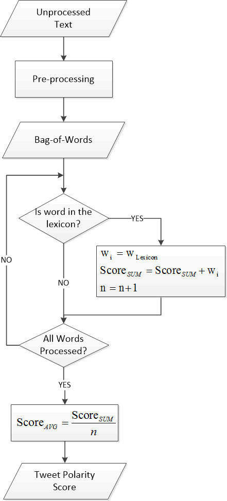
Figure 1: Schematic representation of methodology for the sentiment calculation.

Lexicon-based approach calculates the sentiment of a given text from the polarity of the words or phrases in that text (Turney,, 2002). For this method a lexicon (a dictionary) of words with assigned to them polarity is required. Examples of the existing lexicons include: Opinion Lexicon (Hu and Liu,, 2004), SentiWordNet (Esuli and Sebastiani,, 2006), AFINN Lexicon (Nielsen,, 2011), LoughranMcDonald Lexicon, NRC-Hashtag (Mohammad et al.,, 2013), General Inquirer Lexicon (Stone and Hunt,, 1963).

The sentiment score $Score$ of the text $T$ can be computed as the average of the polarities conveyed by each of the words in the text. The methodology for the sentiment calculation is schematically illustrated in Figure 1 and can be described with the following steps:

• Pre-processing. The text undergoes pre-processing steps that were described in the previous section: POS tagging, stemming, stop-words removal, negation handling, tokenisations into N-grams. The outcome of the pre-processing is a set of tokens or a bag-of-words.

• Checking each token for its polarity in the lexicon. Each word from the bag-of-words is compared against the lexicon. If the word is found in the lexicon, the polarity $w_{i}$ of that word is added to the sentiment score of the text. If the word is not found in the lexicon its polarity is considered to be equal to zero.

• Calculating the sentiment score of the text. After assigning polarity scores to all words comprising the text, the final sentiment score of the text is calculated by dividing the sum of the scores of words caring the sentiment by the number of such words:

  $$Score_{AVG}=\frac{1}{m}\sum_{i=1}^{m}W_{i}.$$ (1)

• The averaging of the score allows to obtain a value of the sentiment score in the range between -1 and 1, where 1 means a strong positive sentiment, -1 means a strong negative sentiment and 0 means that the text is neutral. For example, for the text:

  “A masterful[+0.92] film[0.0] from a master[+1] filmmaker[0.0], unique[+1] in its deceptive[0.0] grimness[0.0], compelling[+1] in its fatalist[-0.84] world[0.0] view[0.0].”

  the sentiment score is calculated as follows:

  $$Score_{AVG}=\frac{0.92+0.0+1+0.0+1+0.0+0.0+1-0.84+0.0+0.0}{5}=0.616.$$

  The sentiment score of 0.616 means that the sentence expresses a positive opinion.

The quality of classification highly depends on the quality of the lexicon. Lexicons can be created using different techniques:

Manually constructed lexicons. The straightforward approach, but also the most time consuming, is to manually construct a lexicon and tag words in it as positive or negative. For example, (Das and Chen,, 2001) constructed their lexicon by reading several thousands of messages and manually selecting words, that were carrying sentiment. They then used a discriminant function to identify words from a training dataset, which can be used for sentiment classifier purposes. The remained words were “expanded” to include all potential forms of each word into the final lexicon. Another example of hand-tagged lexicon is The Multi-Perspective-Question-Answering (MPQA) Opinion Corpus constructed by (Wiebe et al.,, 2005). MPQA is publicly available and consists of 8,222 subjective expressions along with their POS-tags, polarity classes and intensity.

Another resource is The SentiWordNet created by (Esuli and Sebastiani,, 2006). SentiWordNet extracted words from WordNet and gave them probability of belonging to positive, negative or neutral classes, and subjectivity score. Ohana and Tierney demonstrated that SentiWordNet can be used as an important resource for sentiment calculation (Ohana and Tierney,, 2009).

Constructing a lexicon from trained data. This approach belongs to the category of the supervised methods, because a training dataset of labelled sentences is needed. With this method the sentences from the training dataset get tokenised and a bag-of-words is created. The words are then filtered to exclude some parts-of-speech that do not carry sentiment, such as prepositions, for example. The prior polarity of words is calculated according to the occurrence of each word in positive and negative sentences. For example, if a word “success” is appearing more often in the sentences labelled as positive in the training dataset, the prior polarity of this word will be assigned a positive value.

Extending a small lexicon using bootstrapping techniques. Hazivassiloglou and McKeown proposed to extend a small lexicon comprised of adjectives by adding new adjectives which were conjoined with the words from the original lexicon (Hatzivassiloglou and McKeown,, 1997). The technique is based on the syntactic relationship between two adjectives conjoined with the “AND” – it is established that “AND” usually joins words with the same semantic orientation. Example:

“The weather yesterday was nice and inspiring”

Since words “nice” and “inspiring” are conjoined with “AND”, it is considered that both of them carry a positive sentiment. If only the word “nice” was present in the lexicon, a new word “inspiring” would be added to the lexicon. Similarly, (Hatzivassiloglou and McKeown,, 1997) and (Kim and Hovy,, 2004) suggested to expand a small manually constructed lexicon with synonyms and antonyms obtained from NLP resources such as WordNet. The process can be repeated iteratively until it is not possible to find new synonyms and antonyms. Moilanen and Pulman also created their lexicon by semi-automatically expanding WordNet2.1 lexicon (Moilanen and Pulman,, 2007). Other approaches include extracting polar sentences by using structural clues from HTML documents (Kaji and Kitsuregawa,, 2007), recognising opinionated text based on the density of other clues in the text (Wiebe and Wilson,, 2002). After the application of a bootstrapping technique it is important to conduct a manual inspection of newly added words to avoid errors.

5 A Machine Learning Based Approach

A Machine Learning Approach for text classification is a supervised algorithm that analyses data that were previously labelled as positive, negative or neutral; extracts features that model the differences between different classes, and infers a function, that can be used for classifying new examples unseen before. In the simplified form, the text classification task can be described as follows: given a dataset of labelled data $T_{train}=\{\left(t_{1},\ l_{1}\right),\ \dots,\ (t_{n},\ l_{n})\}$ , where each text $t_{i}$ belongs to a dataset $T$ and the label $l_{i}$ is a pre-set class within the group of classes L, the goal is to build a learning algorithm that will receive as an input the training set $T_{train}$ and will generate a model that will accurately classify unlabelled texts.

The most popular learning algorithms for text classification are Support Vector Machines (SVMs) (Cortes and Vapnik,, 1995; Vapnik,, 1995), Naive Bayes (Narayanan et al.,, 2013); Decision Trees (Mitchell,, 1996). Barbosa et al. reports better results for SVMs (Barbosa and Feng,, 2010) while Pak et al. obtained better results for Naive Bayes (Pak and Paroubek,, 2010). In the work by (Dumais et al.,, 1998) a decision tree classifier was shown to perform nearly as well as an SVM classifier.

In terms of the individual classes, some researches (Pang et al.,, 2002) classified texts only as positive or negative, assuming that all the texts carry an opinion. Later (Wilson et al.,, 2005), (Pak and Paroubek,, 2010) and (Barbosa and Feng,, 2010) showed that short messages like tweets and blogs comments often just state facts. Therefore, incorporation of the neutral class into the classification process is necessary.

The process of machine learning text classification can be broken into the following steps:

1. Data Pre-processing. Before training the classifiers each text needs to be pre-processed and presented as an array of tokens. This step is performed according to the process described in section 3.

2. Feature generation. Features are text attributes that are useful for capturing patterns in data. The most popular features used in machine learning classification are the presence or the frequency of n-grams extracted during the pre-processing step. In the presence-based representation for each instance a binary vector is created in which “1” means the presence of a particular n-gram and “0” indicates its absence. In the frequency-based representation the number of occurrences of a particular n-gram is used instead of a binary indication of presence. In cases where text length varies greatly, it might be important to use term frequency (TF) and inverse term frequency (IDF) measures (Rajaraman and Ullman,, 2011). However, in short messages like tweets words are unlikely to repeat within one instance, making the binary measure of presence as informative as the counts (Ikonomakis et al.,, 2005).

   Apart from the n-grams, additional features can be created to improve the overall quality of text classification. The most common features that are used for this purpose include:

   • Number of words with positive/negative sentiment;

   • Number of negations;

   • Length of a message;

   • Number of exclamation marks;

   • Number of different parts-of-speech in a text (for example, number of nouns, adjectives, verbs);

   • Number of comparative and superlative adjectives.

3. Feature selection. Since the main features of a text classifier are N-grams, the dimensionality of the feature space grows proportionally to the size of the dataset. This dramatical growth of the feature space makes it in most cases computationally infeasible to calculate all the features of a sample. Many features are redundant or irrelevant and do not significantly improve the results. Feature selection is the process of identifying a subset of features that have the highest predictive power. This step is crucial for the classification process, since elimination of irrelevant and redundant features allows to reduce the size of feature space increasing the speed of the algorithm, avoiding overfitting as well as contributing to the improved quality of classification.

   There are three basic steps in feature selection process (Dash and Liu,, 1997)

   1. Search procedure. A process that generates a subset of features for evaluation. A procedure can start with no variables and add them one by one (forward selection) or with all variables and remove one at each step (backward selection), or features can be selected randomly (random selection).

   2. Evaluation procedure. A process of calculating a score for a selected subset of features. The most common metrics for evaluation procedure are: Chi-squared, Information Gain, Odds Ratio, Probability Ratio, Document Frequency, Term Frequency. An extensive overview of search and evaluation methods is presented in (Ladha and Deepa, 2011a, ; Forman,, 2003).

   3. Stopping criterion. The process of feature selection can be stopped based on a: i) search procedure, if a predefined number of features was selected or predefined number of iterations was performed; ii) evaluation procedure, if the change of feature space does not produce a better subset or if optimal subset was found according to the value of evaluation function.

4. Learning an Algorithm. After feature generation and feature selection steps the text is represented in a form that can be used to train an algorithm. Even though many classifiers have been tested for sentiment analysis purposes, the choice of the best algorithm is still not easy since all methods have their advantages and disadvantages (see (Marsland,, 2011) for more information on classifiers).

   Decision Trees (Mitchell,, 1996). A decision tree text classifier is a tree in which non-leaf nodes represent a conditional test on a feature, branches denote the outcomes of the test, and leafs represent class labels. Decision trees can be easily adapted to classifying textual data and have a number of useful qualities: they are relatively transparent, which makes them simple to understand; they give direct information about which features are important in making decisions, which is especially true near the top of the decision tree. However, decision trees also have a few disadvantages. One problem is that trees can be easily overfitted. The reason lies in the fact that each branch in the decision tree splits the training data, thus, the amount of training data available to train nodes located in the bottom of the tree, decreases. This problem can be addressed by using the tree pruning. The second weakness of the method is the fact that decision trees require features to be checked in a specific order. This limits the ability of an algorithm to exploit features that are relatively independent of one another.

   Naive Bayes (Narayanan et al.,, 2013) is frequently used for sentiment analysis purposes because of its simplicity and effectiveness. The basic concept of the Naive Bayes classifier is to determine a class (positive negative, neutral) to which a text belongs using probability theory. In case of the sentiment analysis there will be three hypotheses: one for each sentiment class. The hypothesis that has the highest probability will be selected as a class of the text. The potential problem with this approach emerges if some word in the training set appears only in one class and does not appear in any other classes. In this case, the classifier will always classify text to that particular class. To avoid this undesirable effect Laplace smoothing technique may be applied.

   Another very popular algorithm is Support Vector Machines (SVMs) (Cortes and Vapnik,, 1995; Vapnik,, 1995). For the linearly separable two-class data, the basic idea is to find a hyperplane, that not only separates the documents into classes, but for which the Euclidian distance to the closest training example, or margin, is as large as possible. In a three-class sentiment classification scenario, there will be three pair-wise classifications: positive-negative, negative-neutral, positive-neutral. The method has proved to be very successful for the task of text categorization (Joachims,, 1999; Dumais et al.,, 1998) since it can handle very well large feature spaces, however, it has low interpretability and is very computationally expensive, because it involves calculations of discretisation, normalization and dot product operations.

5. Model Evaluation. After the model is trained using a classifier it should be validated, typically, using a cross-validation technique, and tested on a hold-out dataset. There are several metrics defined in information retrieval for measuring the effectiveness of classification, among them are:

   • Accuracy: as described by (Kotsiantis,, 2007), accuracy is “the fraction of the number of correct predictions over the total number of predictions”.

   • Error rate: measures the number of incorrectly predicted instance against the total number of predictions.

   • Precision: shows the proportion of how many instances the model classified correctly to the total number of true positive and true negative examples. In other words, precision shows the exactness of the classifier with respect to each class.

   • Recall: represents the proportion of how many instances the model classified correctly to the total number of true positives and false negatives. Recall shows the completeness of the classifier with respect to each class.

   • F-score: (Rijsbergen,, 1979) defined the F1-score as the harmonic mean of precision and recall:

   $$\mbox{{F-Score}}=\frac{2*Precision*Recall}{Precision+Recall}.$$ (2)

   Depending on the nature of the task, one may use accuracy, error rate, precision, recall or F-score as a metric or some mixture of them. For example, for unbalanced datasets, it was shown that precision and recall can be better metrics for measuring classifiers performance (Manning and Schütze,, 1999). However, sometimes one of these metrics can increase at the expense of the other. For example, in the extreme cases the recall can reach to 100%, but precision can be very low. In these situations the F-score can be a more appropriate measure.

6 Application of Lexicon and Machine Learning Methods for Twitter Sentiment Classification

Here we provide an example of implementation of the lexicon based approach and the machine learning approach on a case-study. We use benchmark datasets from SemEval-2013 Competition, Task 2: Sentiment Analysis in Twitter, that included two subtasks: A) an expression-level classification, B) a message-level classification (Nakov et al.,, 2013). Our interest is in subtask B: “Given a message, decide whether it is of positive, negative, or neutral sentiment. For messages conveying both a positive and a negative sentiment, whichever is the stronger one was to be chosen” (Nakov et al.,, 2013). After training and evaluating our algorithm on the training and test datasets provided by SemEval-2013, Task-2 (please, refer to Figure 2 for statistics of positive, negative and neutral messages for training and test datasets), we compare our results against the results of 44 participated teams and 149 submissions.

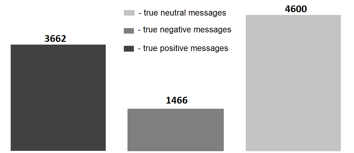
(a)

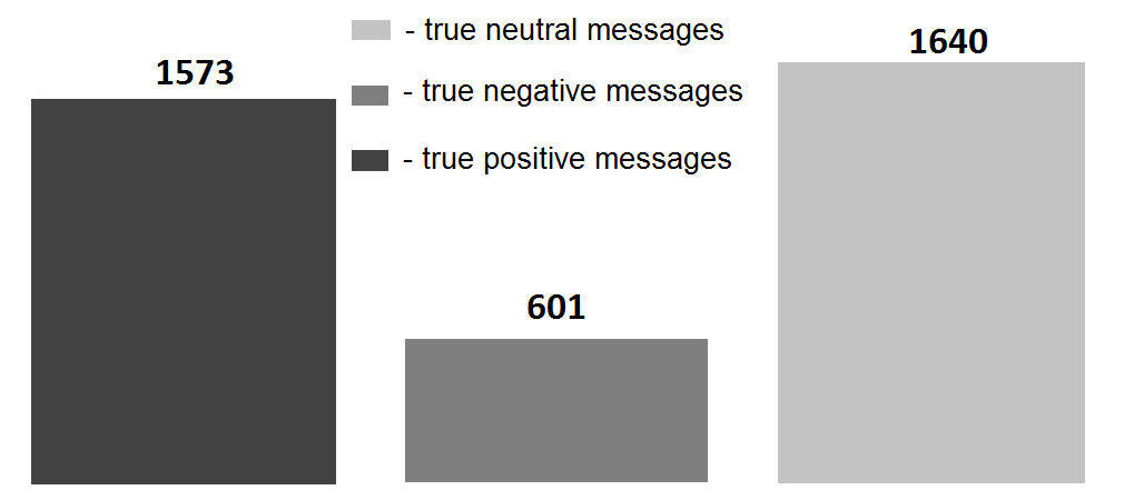
(b)

Figure 2: Statistics of a) training dataset and b) test datset from SemEval-2013 competition, Task 2-B (Nakov et al.,, 2013). Dark grey bar on the left represents the proportion of positive tweets in the dataset, grey bar in the middle shows the proportion of negative tweets and light grey bar on the right reflects the proportion of neutral sentences.

The second example of application of our algorithm to a large dataset of 42,803,225 Twitter messages related to retail companies is presented in (Souza et al.,, 2015) and investigates the relationship between Twitter sentiment and stock returns and volatility.

6.1 Pre-processing

We performed pre-processing steps as described in section 3. For the most of the steps we used the machine learning software WEKA. WEKA was developed in the university Wakaito and provides implementations of many machine learning algorithms. Since it is an open source tool and has an API, WEKA algorithms can be easily embedded within other applications.

Stemming and lemmatisation. The overall impact of stemming depends on the dataset and stemming algorithm. WEKA contains implementation of a SnowballStemmer (Porter,, 2002) and LovinsStemmer (Lovins,, 1968). After testing both implementations we discovered that the accuracy of the sentiment classification was decreased after applying both stemming algorithms, therefore, stemming operation was avoided in the final implementation of the sentiment analysis algorithm.

Stop-words Removal. WEKA provides a file with a list of words, which should be considered as stop-words. The file can be adjusted to ones needs. In our study we used a default WEKA stop-list file.

Table 2: Example POS tags.

@ Tag	Description
@ at-mentions	Is used to identify the user- recipient of the tweet
U	URL or email address
#	Hashtag to identify the topic of the discussion or a category
~	Discourse marker. Indicates, that message is the continuation of the previous tweet
E	Emoticons , , etc.
G	Abbreviations, shortenings of words

Table 3: Example of ArkTweetNLP (Gimpel et al.,, 2011) tagger in practice.

Sentence: ikr smh he asked fir yo last name so he can add u on fb lololol word tag confidence ikr ! 0.8143 smh G 0.9406 he O 0.9963 asked V 0.9979 fir P 0.5545 yo D 0.6272 last A 0.9871 name N 0.9998 so P 0.9838 he O 0.9981 can V 0.9997 add V 0.9997 u O 0.9978 on P 0.9426 fb ^ 0.9453 lololol ! 0.9664 “ikr” means “I know, right?”, tagged as an interjection. “so” is being used as a subordinating conjunction, which our coarse tagset denotes P. “fb” means “Facebook”, a very common proper noun (^). “yo” is being used as equivalent to “your”; our coarse tagset has posessive pronouns as D. “fir” is a misspelling or spelling variant of the preposition for. Perhaps the only debatable errors in this example are for ikr and smh (“shake my head”): should they be G for miscellaneous acronym, or ! for interjection?

Part-of-Speech Tagging (POS). In the current study we tested performance of multiple existing pos-taggers: Stanford Tagger, Illinois Tagger, OpenNLP, LingPipe POS Tagger, Unsupos, ArkTweetNLP, Berkeley NLP Group Tagger. We finally chose to use ArkTweetNLP library developed by the team of researchers from Carnegie Mellon University (Gimpel et al.,, 2011) since it was trained on a Twitter dataset. ArkTweetNLP developed 25 POS tags, with some of them specifically designed for special Twitter symbols, such as hashtags, at-mentions, retweets, emoticons, commonly used abbreviations (see Table 2 for some tags examples). An example of how ArkTweetNLP tagger works in practice is presented in Table 3.

As the result of POS-tagging in our study, we filtered out all words that did not belong to one of the following categories: N(common noun), V(verb), A(adjective), R(adverb), !(interjection), E(emoticon), G(abbreviations, foreign words, possessive endings).

Negations Handling. We implemented negation handling using simple, but effective strategy: if negation word was found, the sentiment score of every word appearing between a negation and a clause-level punctuation mark (.,!?:;) was reversed (Pang et al.,, 2002). There are, however, some grammatical constructions in which a negation term does not have a scope. Some of these situations we implemented as exceptions:

Exception Situation 1: Whenever a negation term is a part of a phrase that does not carry negation sense, we consider that the scope for negation is absent and the polarity of words is not reversed. Examples of these special phrases include “not only”, “not just”, “no question”, “not to mention” and “no wonder”.

Exception Situation 2: A negation term does not have a scope when it occurs in a negative rhetorical question. A negative rhetorical question is identified by the following heuristic. (1) It is a question; and (2) it has a negation term within the first three words of the question. For example:
“Did not I enjoy it?”
“Wouldn’t you like going to the cinema?”

Tokenisation into N-grams. We used WEKA tokeniser to extract uni-grams and bi-grams from the Twitter dataset.

6.2 Lexicon Approach

Automatic Lexicon Generation.

In this study we aimed to create a lexicon specifically oriented for sentiment analysis of Twitter messages. For this purpose we used the approach described in 4: “Constructing a lexicon from trained data” and the training dataset from Mark Hall (Hall,, 2012) that is comprised of manually labelled 41403 positive Twitter messages and 8552 negative Twitter messages. The method to generate a sentiment lexicon was implemented as follows:

1. Pre-processing of the dataset: POS tags were assigned to all words in the dataset; words were lowered in case; BOW was created by tokenising the sentences in the dataset.

2. The number of occurrences of each word in positive and negative sentences from the training dataset was calculated.

3. The positive polarity of each word was calculated by dividing the number of occurrences in positive sentences by the number of all occurrences:

   $$positiveSentScore=\ \frac{\#Positive\ sentences}{\left(\#Positive\ sentences+\#Negative\ sentences\right)}.$$ (3)

   For example, we calculated that the word “pleasant” appeared 122 times in the positive sentences and 44 times in the negative sentences. According to the formula, the positive sentiment score of the word “pleasant” is

   $$positiveSentScore=\ \frac{122\ }{\left(122+44\right)}=\ 0.73.$$

   Similarly, the negative score for the word “pleasant” can be calculated by dividing the number of occurrences in negative sentences by the total number of mentions

   $$negativeSentScore=\ \frac{\#Negative\ sentences}{\left(\#Positive\ sentences+\#Negative\ sentences\right)},$$ (4)

   $$negativeSentScore=\ \frac{44\ }{\left(122+44\right)}=\ 0.27.$$

   Based on the positive score of the word we can make a decision about its polarity: the word is considered positive, if its positive score is above 0.6; the word is considered neutral, if its positive score is in the range [0.4; 0.6]; the word is considered negative, if the positive score is below 0.4. Since the positive score of the word “pleasant” is 0.73, it is considered to carry positive sentiment. Sentiment scores of some other words from the experiment are presented in Table 4.

   Table 4: Example of sentiment scores of words in the automatically generated lexicon.

   	GOOD	BAD	LIKE
   Positive Score	0.675	0.213	0.457
   Negative Score	0.325	0.787	0.543

   We can observe from the table that the words “GOOD” and “BAD” have strongly defined positive and negative scores, as we would expect. The word “LIKE” has polarity scores ranging between 0.4 and 0.6 indicating its neutrality. To understand why the “neutral” label for the word “LIKE” was assigned we investigate the semantic role of this word in English language:

   1. Being a verb to express preference. For example: “I like ice-cream”.

   2. Being a preposition for the purpose of comparison. For example: “This town looks like Brighton.”

   The first sentence has positive sentiment, however can easily be transformed into a negative sentence: “I don’t like ice-cream”. This demonstrates that the word “LIKE” can be used with equal frequency for expressing positive and negative opinions. In the second example the word “LIKE” is playing a role of a preposition and does not effect the overall polarity of the sentence. Thus, the word “LIKE” is a neutral word and was correctly assigned a neutral label using the approach described above.

   In our study all words from the Bag-of-Words with a polarity in the range [0.4; 0.6] were removed, since they do not help to classify the text as positive or negative. The sentiment scores of the words were mapped into the range [-1;1] by using the following formula:

   $$PolarityScore=2*positiveSentScore-1.$$ (5)

   According to this formula, the word “LIKE”, obtained a score 0.446 * 2 -1 = -0.1, which indicates the neutrality of the word. In case when the word is extremely positive and had a $positiveSentScore$ of 1, the mapped score will be positive: 1 * 2 – 1 = 1. If the word is extremely negative and has the $positiveSentScore$ equal to 0, the mapped score will be negative: 0 * 2 - 1 = -1.

Lexicons Combinations.

Since the role of emoticons for expressing opinion online is continuously increasing, it is crucial to incorporate emoticons into lexicons used for sentiment analysis. Hogenboom et al. showed that incorporation of the emoticons into lexicon can significantly improve the accuracy of classification (Hogenboom et al.,, 2013). Apart from emoticons, new slang words and abbreviations are constantly emerging and need to be accounted for when performing sentiment analysis. However, most of the existing public lexicons do not contain emoticons and social-media slang, on the contrary, emoticons and abbreviations are often being removed as typographical symbols during the first stages of pre-processing.

Table 5: Example of tokens from our EMO lexicon along with their polarity. Tokens represent emoticons, abbreviations and slang words that are used in social-media to express emotions.

Emoticon	Score	Emoticon	Score	Abbreviation	Score	Abbreviation	Score
l-)	1	[-(	-1	lol	1	dbeyr	-1
:-}	1	T_T	-1	ilum	1	iwiam	-1
x-d	1	:-((	-1	iyqkewl	1	nfs	-1
;;-)	1	:-[	-1	iwalu	1	h8ttu	-1
=]	1	:(((	-1	koc	1	gtfo	-1

In this study we manually constructed a lexicon of emoticons, abbreviations and slang words commonly used in social-media to express emotions (EMO). Example of tokens from our lexicon are presented in Table 5. We aimed to analyse how performance of the classic opinion lexicon (OL) (Hu and Liu,, 2004) can be improved by enhancing it with our EMO lexicon. We also expanded the lexicon further by incorporating words from the automatically created lexicon (AUTO). The process of automatic lexicon creation was described in detail in the previous section.

With opinion lexicon (OL) serving as a baseline, we compared the performance of some lexicon combinations as shown in Table 6:

Table 6: Combinations of lexicons tested

	Lexicons combinations
1.	OL
2.	OL + EMO
3.	OL + EMO + AUTO

Sentiment Score Calculation.

In this study we calculate sentiment scores of tweets as described in section 2 using Equation 1. We also propose an alternative measure based on the logarithm of the standard score. We normalise the logarithmic score in such a way that the values range between [-1; 1] with -1 being the most negative score and 1 being the most positive score (see 6).

$$Score_{Log{10}}=\begin{cases}{sign}({Score}_{AVG})Log_{10}(\mid 10{Score}_{AVG}\mid),&\text{if }\mid{Score}_{AVG}\mid>0.1,\\ 0,&\text{otherwise}\end{cases}$$ (6)

Lexicon Performance Results.

The analysis of performance of our algorithm was conducted on the test dataset from SemEval-2013, Task 2-B (Nakov et al.,, 2013) (see Figure 2b). Figure 3 presents the results for the three different lexicons using the Simple Average as the sentiment score (Equation 1). The values of the sentiment score range from -1 to 1. The colors of the bars represent the true labels of the tweets: dark grey stands for positive messages, light grey for neutral messages and medium grey stands for negative messages. In the case of perfect classification, we would obtain a clear separation of the colors. However, from Figure 3 we can see that classification for all three lexicons was not ideal. For example, all lexicons made the biggest mistake in misclassifying neutral messages (we can see that light grey color is present for the sentiment scores of -1 and 1 in all three histograms, indicating that some of neutral messages were classified as positive or negative). This phenomenon can be explained with the fact that even neutral messages often contain one or more polarity words, which leads to the final score of the message being a value different from 0 and being classified as positive or negative.

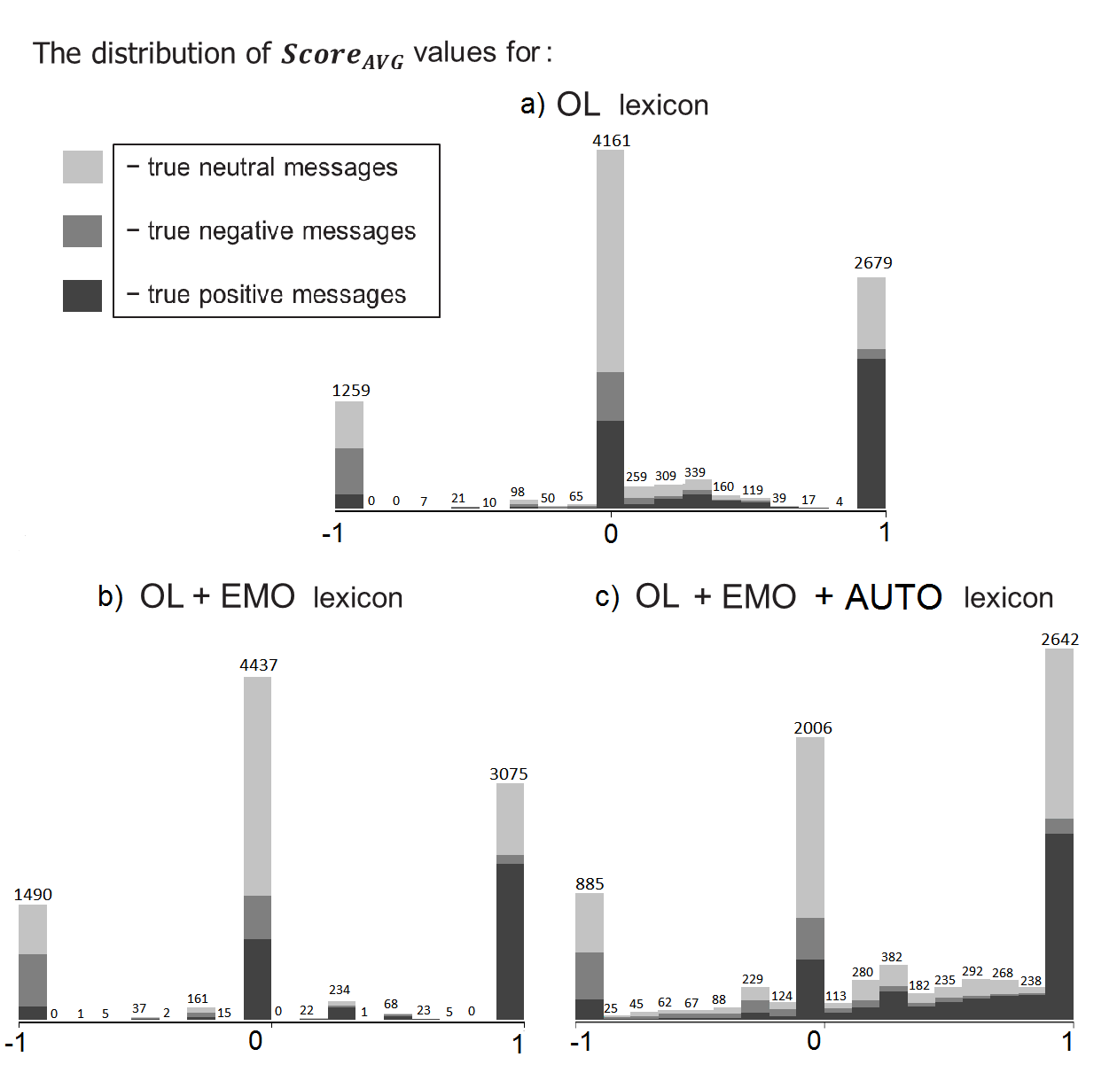
Figure 3: Histograms of sentiment scores for different lexicon combinations using the Simple Average Score. The colors of the bars represent the true labels of the tweets: dark grey stands for positive messages, light grey for neutral messages and medium grey stands for positive messages.

The results based on the logarithmic approach (Equation 6) reveal that positive, negative and neutral classes became more defined (Figure 4). Indeed, the logarithmic score makes it easier to set up the thresholds for assigning labels to different classes, thus, we can conclude that using a logarithmic score for calculating sentiment is more appropriate than using a simple average score.

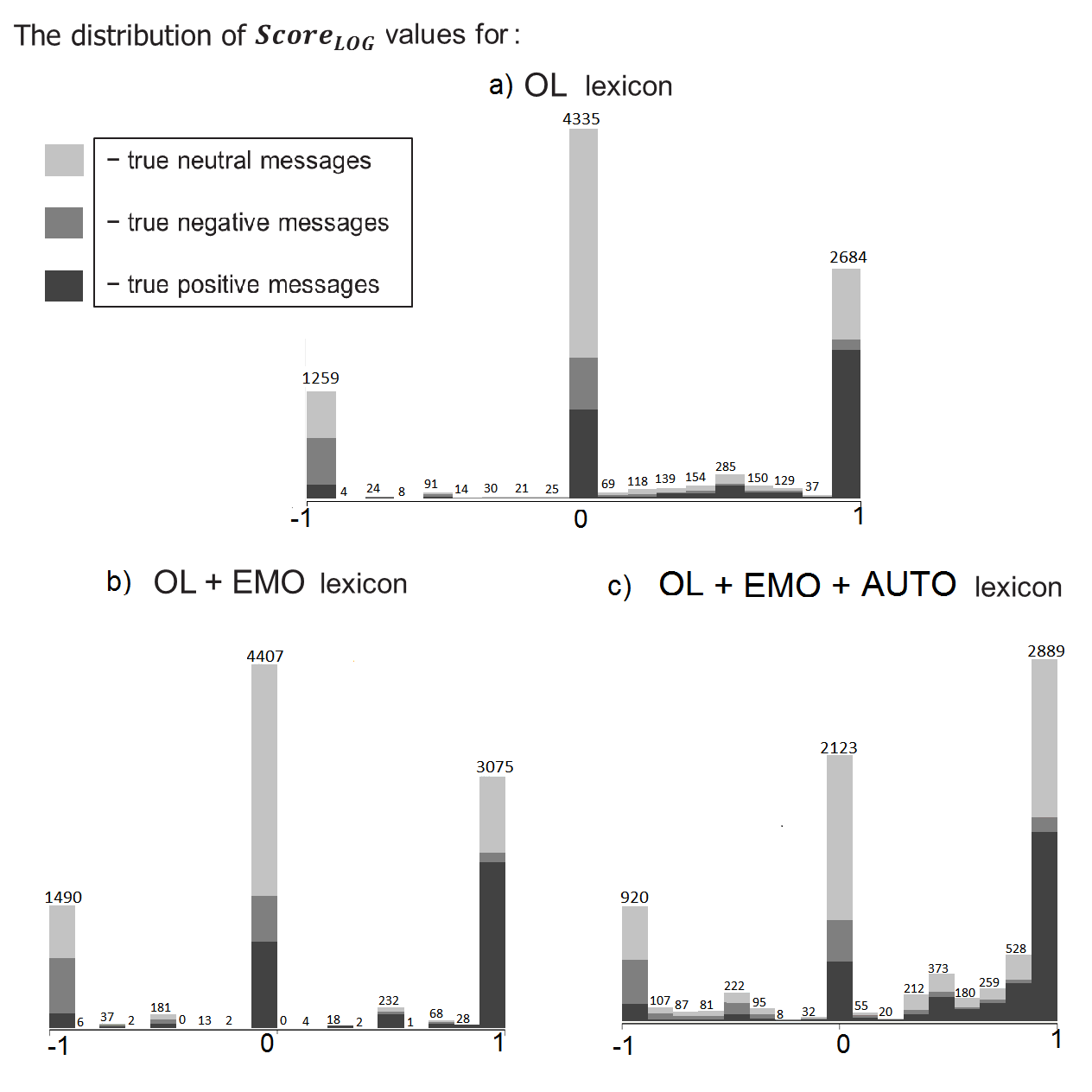
Figure 4: Histograms of sentiment scores for different lexicon combinations using the Logarithmic Score. The colors of the bars represent the true labels of the tweets: dark grey stands for positive messages, light grey for neutral messages and medium grey stands for positive messages.

To compare the performance of three lexicon combinations we need to assign positive, negative or neutral labels to the tweets based on the calculated sentiment scores, and compare the predicted labels against the true labels of tweets. For this purpose we employ a k-means clustering algorithm, using Simple Average and Logarithmic scores as features. The results of K-means clustering for the 3 lexicons and 2 types of sentiment scores are reported in Table 7.

Table 7: Results of K-Means clustering for different lexicon combinations.

Accuracy	OL	OL + EMO	OL + EMO + AUTO
${Score}_{AVG}$	57.07%	60.12%	51.33%
$Score_{Log{10}}$	58.43%	61.74%	52.38%

As shown in Table 7 the lowest accuracy of classification for both types of scores corresponded to the biggest lexicon (OL + EMO + AUTO). This result can be related to a noisy nature of Twitter data. Training a lexicon on noisy data could have introduced ambiguity regarding the sentiment of individual words. Thus, automatic generation of the lexicon (AUTO) based on Twitter labelled data cannot be considered a reliable technique. The small OL lexicon showed better results since it consisted mainly of adjectives that carry strong positive or negative sentiment that are unlikely to cause ambiguity. The highest accuracy of classification 61.74% was achieved using the combination of OL and EMO lexicons (OL + EMO) and a logarithmic score. This result confirms that enhancing the lexicon for Twitter sentiment analysis with emoticons, abbreviations and slang words increases the accuracy of classification. It is important to notice that the Logarithmic Score provided an improvement of 1.36% over the Simple Average Score.

6.3 Machine Learning Approach

We performed Machine Learning based sentiment analysis. For this purpose we used the machine learning package WEKA.

Pre-processing/cleaning the data.

Before training the classifiers the data needed to be pre-processed and this step was performed according to the general process described in section 3. Some additional steps that had to be performed:

• Filtering. Some syntactic constructions used in Twitter messages are not useful for sentiment detection. These constructions include URLs, @-mentions, hashtags, RT-symbols and they were removed during the pre-processing step.

• Tokens replacements. The words that appeared to be under the effect of the negation words were modified by adding a suffix _NEG to the end of those words.

  For example, the phrase I don’t want. was modified to I don’t want_NEG.

  This modification is important, since each word in a sentence serves a purpose of a feature during the classification step. Words with _NEG suffixes increase the dimensionality of the feature space, but allow the classifier to distinguish between words used in the positive and in the negative context.

  When performing tokenisation, the symbols ():;, among others are considered to be delimiters, thus most of the emoticons could be lost after tokenisation. To avoid this problem positive emoticons were replaced with pos_emo and negative were replaced with neg_emo. Since there are many variations of emoticons representing the same emotions depending on the language and community, the replacement of all positive lexicons by ‘pos_emo’ and all negative emoticons by ‘neg_emo’ also achieved the goal of significantly reducing the number of features.

Feature Generation.

The following features were constructed for the purpose of training a classifier:

• N-grams: we transformed the training dataset into the bag-of-ngrams taking into account only the presence/absence of unigrams. Using “n-grams frequency” would not be logical in this particular experiment, since Twitter messages are very short, and a term is unlikely to appear in the same message more than once;

• Lexicon Sentiment: the sentiment score obtained during the lexicon based sentiment analysis as described in 6;

• Elongated words number: the number of words with one character repeated more than 2 times, e.g. ’soooo’;

• Emoticons: presence/absence of positive and negative emoticons at any position in the tweet;

• Last token: whether the last token is a positive or negative emoticon;

• Negation: the number of negated contexts;

• POS: the number of occurrences for each part-of-speech tag: verbs, nouns, adverbs, at-mentions, abbreviations, URLs, adjectives and others

• Punctuation marks: the number of occurrences of punctuation marks in a tweet;

• Emoticons number: the number of occurrences of positive and negative emoticons;

• Negative tokens number: total count of tokens in the tweet with logarithmic score less than 0;

• Positive tokens number: total count of tokens in the tweet with logarithmic score greater than 0;

Feature Selection.

After performing the feature generation step described above a feature space comprising 1826 features was produced. The next important step for improving classification accuracy is the selection of the most relevant features from this feature space. To this purpose we used Information Gain evaluation algorithm and a Ranker search method (Ladha and Deepa, 2011b, ). Information Gain measures the decrease in entropy when the feature is present vs absent, while Ranker ranks the features based on the amount of reduction in the objective function. We used features for which the value of information gain was above zero. As the result, a subset of 528 features was selected.

Table 8: Example of top selected features.

TOP FEATURES	11. great	22. fun	33. hope
1. LexiconScore	12. posV	23. lastTokenScore	34. thanks
2. maxScore	13. happy	24. i love	35. luck
3. posR	14. love	25. don	36. best
4. minScore	15. excited	26. don’t	37. i don’t
5. negTokens	16. can’t	27. amazing	38. looking forward
6. good	17. i	28. fuck	39. sorry
7. posE	18. not	29 love you	40. didn’t
8. posN	19. posA	30. can	41. hate
9. posU	20. posElongWords	31. awesome	42. …

Some of the top selected features are displayed in Table 8, revealing that the “Lexicon Sentiment” feature, described in the previous section as a “Lexicon Sentiment”, is located at the top of the list. This important result demonstrates that the “Lexicon Sentiment” plays a leading role in determining the final sentiment polarity of the sentence. Other highly ranked features included: minimal and maximum scores, number of negated tokens, number of different parts-of-speech in the message. To validate the importance of the “Lexicon Sentiment” feature and other manually constructed features, we performed cross-validation tests according to two scenarios: i) in the first scenario (Table 9) we trained three different classifiers using only N-grams as features; ii) in the second scenario (Table 10) we trained the models using traditional N-grams features in combination with the “Lexicon Sentiment” feature and other manually constructed features: number of different parts-of-speech, number of emoticons, number of elongated words. Tests were performed on a movie review dataset “Sentence Polarity Dataset v 1.0 ” released by Bo Pang and Lillian Lee in 2005 and comprised of 5331 positive and 5331 negative processed sentences.

As it can be observed from tables 9 and 10, the addition of the “Lexicon Sentiment” feature and other manually constructed features allowed to increase all performance measures significantly for 3 classifies. For example, the accuracy of Naive Bayes classifier was increased by 7%, accuracy of Decision Trees was increased by over 9%, and the accuracy of SVM improved by 4.5%.

Table 9: Scenario 1: 5-fold cross-validation test on a movies reviews dataset using only N-grams as features.

Method	Tokens Type	Folds Number	Accuracy	Precision	Recall	F-Score
Naive Bayes	uni/bigrams	5	81.5%	0.82	0.82	0.82
Decision Trees	uni/bigrams	5	80.57%	0.81	0.81	0.81
SVM	uni/bigrams	5	86.62%	0.87	0.87	0.87

Table 10: Scenario 2: 5-fold cross-validation test on a movies reviews dataset using traditional N-grams features in combination with manually constructed features: lexicon sentiment score, number of different parts-of-speech, number of emoticons, number of elongated words, etc.

Method	Tokens Type	Folds Number	Accuracy	Precision	Recall	F-Score
Naive Bayes	uni/bigrams	5	88.54%	0.89	0.86	0.86
Decision Trees	uni/bigrams	5	89.9%	0.90	0.90	0.90
SVM	uni/bigrams	5	91.17%	0.91	0.91	0.91

Training the Model, Validation and Testing.

Machine Learning Supervised approach requires a labelled training dataset. We used a publicly available training dataset (Figure 2a) from SemEval-2013 competition, Task 2-B (Nakov et al.,, 2013).

Each of the tweets from the training set was expressed in terms of its attributes. As the result, $n$ by $m$ binary matrix was created, where $n$ is the number of training instances and $m$ is the number of features. This matrix was used for training different classifiers: Naive Bayes, Support Vector Machines, Decision trees. It is important to notice that the training dataset was highly unbalanced with the majority of neutral messages (Figure 2a). In order to account for this unbalance we trained a cost-sensitive SVM model (Ling and Sheng,, 2007). Cost-Sensitive classifier allows to minimize the total cost of classification by putting a higher cost on a particular type of error (in our case, misclassifying positive and negative messages as neutral).

As the next step we tested the models on an unseen before test set (Figure 2b) from SemEval-2013 Competition (Nakov et al.,, 2013) and compared our results against the results of 44 teams that took part in the SemEval-2013 competition. While the classification was performed for 3 classes (pos, neg, neutral), the evaluation metric was F-score (Equation 2) between positive and negative classes.

Table 11: F-score results of our algorithm using different classifiers. The test was performed on a test dataset from SemEval Competition-2013, Task 2-B (Nakov et al.,, 2013).

Classifier	Naive Bayes	Decision Trees	SVM	Cost Sensitive SVM
F-SCORE	0.64	0.62	0.66	0.73

Table 12: Fscore results of SemEval Competition-2013, Task 2-B (Nakov et al.,, 2013).

TEAM NAME	F-SCORE
NRC-Canada	0.6902
GUMLTLT	0.6527
TEREGRAM	0.6486
AVAYA
BOUNCE	0.6353
KLUE	0.6306
AMI and ERIC	0.6255
FBM	0.6117
SAIL
AVAYA	0.6084
SAIL	0.6014
UT-DB	0.5987
FBK-irst	0.5976

Our results for different classifiers are presented in Table 11. We can observe that the Decision Tree algorithm had the lowest F-score of 62%. The reason may lay in a big size of the tree needed to incorporate all of the features. Because of the tree size, the algorithm needs to traverse multiple nodes until it reaches the leaf and predicts the class of the instance. This long path increases the probability of mistakes and thus decreases the accuracy of the classifier. Naive Bayes and SVM produced better scores of 64% and 66% respectively. The best model was a Cost-sensitive SVM that allowed to achieve the F-measure of 73%. This is an important result, providing evidence that accounting for the unbalance in the training dataset allows to improve model performance significantly. Comparing our results with the results of the competition (Table 12), we can conclude that our algorithm based on the Cost-sensitive SVM would had produced the best results scoring 4 points higher than the winner of that competition.

7 Conclusion

In this paper we have presented the review of two main approaches for sentiment analysis, a lexicon based method and a machine learning method.

In the lexicon based approach we compared the performance of three lexicons: i) an Opinion lexicon (OL); ii) an Opinion lexicon enhanced with manually created corpus of emoticons, abbreviations and social-media slang expressions (OL + EMO); iii) OL + EMO further enhanced with automatically generated lexicon (OL + EMO + AUTO). We showed that on a benchmark Twitter dataset, OL + EMO lexicon outperforms both, the traditional OL and a larger OL + EMO + AUTO lexicon. These results demonstrate the importance of incorporating expressive signals such as emoticons, abbreviations and social-media slang phrases into lexicons for Twitter analysis. The results also show that larger lexicons may yield a decrease in performance due to ambiguity of words polarity and increased model complexity (agreeing with (Ghiassi et al.,, 2013)).

In the machine learning approach we propose to use a lexicon sentiment obtained during the lexicon based classification as an input feature for training classifiers. The ranking of all features based on the information gain scores during the feature selection process revealed that the lexicon feature appeared on the top of the list, confirming its relevance in sentiment classification. We also demonstrated that in case of highly unbalanced datasets the utilisation of cost-sensitive classifiers improves accuracy of class prediction: on the benchmark Twitter dataset a cost-sensitive SVM yielded 7% increase in performance over a standard SVM.

References

- Aisopos et al., (2012) Aisopos, F., Papadakis, G., Tserpes, K., and Varvarigou, T. (2012). Content vs. context for sentiment analysis: A comparative analysis over microblogs. In Proceedings of the 23rd ACM Conference on Hypertext and Social Media, HT ’12, pages 187–196, New York, NY, USA. ACM.
- Antenucci et al., (2014) Antenucci, D., Cafarella, M., Levenstein, M. C., Ré, C., and Shapiro, M. (2014). Using social media to measure labor market flows. http://www.nber.org/papers/w20010. Accessed: 2015-04-10.
- Asur and Huberman, (2010) Asur, S. and Huberman, B. A. (2010). Predicting the future with social media. In Proceedings of the 2010 IEEE/WIC/ACM International Conference on Web Intelligence and Intelligent Agent Technology - Volume 01, WI-IAT ’10, pages 492–499, Washington, DC, USA. IEEE Computer Society.
- Barbosa and Feng, (2010) Barbosa, L. and Feng, J. (2010). Robust sentiment detection on twitter from biased and noisy data. In Proceedings of the 23rd International Conference on Computational Linguistics: Posters, COLING ’10, pages 36–44, Stroudsburg, PA, USA. Association for Computational Linguistics.
- Basili et al., (2000) Basili, R., Moschitti, A., and Pazienza, M. T. (2000). Language-Sensitive Text Classification. In Proceeding of RIAO-00, 6th International Conference “Recherche d’Information Assistee par Ordinateur”, pages 331–343, Paris, France.
- Benamara et al., (2007) Benamara, F., Irit, S., Cesarano, C., Federico, N., and Reforgiato, D. (2007). Sentiment Analysis: Adjectives and Adverbs are better than Adjectives Alone. In In Proc of Int Conf on Weblogs and Social Media.
- Bing, (2012) Bing, L. (2012). Sentiment analysis: A fascinating problem. In Sentiment Analysis and Opinion Mining, pages 7–143. Morgan and Claypool Publishers.
- Bollen et al., (2010) Bollen, J., Mao, H., and Zeng, X. (2010). Twitter mood predicts the stock market. In CoRR, volume abs/1010.3003.
- Caropreso et al., (2001) Caropreso, M. F., Matwin, S., and Sebastiani, F. (2001). A learner-independent evaluation of the usefulness of statistical phrases for automated text categorization. In Chin, A. G., editor, Text Databases and Document Management, pages 78–102, Hershey, PA, USA. IGI Global.
- Carvalho et al., (2014) Carvalho, J., Prado, A., and Plastino, A. (2014). A statistical and evolutionary approach to sentiment analysis. In Proceedings of the 2014 IEEE/WIC/ACM International Joint Conferences on Web Intelligence (WI) and Intelligent Agent Technologies (IAT) - Volume 02, WI-IAT ’14, pages 110–117, Washington, DC, USA. IEEE Computer Society.
- Cortes and Vapnik, (1995) Cortes, C. and Vapnik, V. (1995). Support-vector networks. In Machine Learning, volume 20, pages 273–297, Hingham, MA, USA. Kluwer Academic Publishers.
- Councill et al., (2010) Councill, I. G., McDonald, R., and Velikovich, L. (2010). What’s great and what’s not: Learning to classify the scope of negation for improved sentiment analysis. In Proceedings of the Workshop on Negation and Speculation in Natural Language Processing, NeSp-NLP ’10, pages 51–59, Stroudsburg, PA, USA. Association for Computational Linguistics.
- Das and Chen, (2001) Das, S. and Chen, M. (2001). Yahoo! for amazon: Extracting market sentiment from stock message boards. In Asia Pacific Finance Association Annual Conf. (APFA).
- Dash and Liu, (1997) Dash, M. and Liu, H. (1997). Feature selection for classification. In Intelligent data analysis, volume 1, pages 131–156. No longer published by Elsevier.
- Diederich et al., (2003) Diederich, J., Kindermann, J., Leopold, E., and Paass, G. (2003). Authorship attribution with support vector machines. In Applied Intelligence, volume 19, pages 109–123, Hingham, MA, USA. Kluwer Academic Publishers.
- Ding et al., (2008) Ding, X., Liu, B., and Yu, P. S. (2008). A holistic lexicon-based approach to opinion mining. In Proceedings of the 2008 International Conference on Web Search and Data Mining, WSDM ’08, pages 231–240, New York, NY, USA. ACM.
- Dumais et al., (1998) Dumais, S., Platt, J., Heckerman, D., and Sahami, M. (1998). Inductive learning algorithms and representations for text categorization. In CIKM ’98: Proceedings of the seventh international conference on Information and knowledge management, pages 148–155, New York, NY, USA. ACM.
- Esuli and Sebastiani, (2006) Esuli, A. and Sebastiani, F. (2006). Sentiwordnet: A publicly available lexical resource for opinion mining. http://www.bibsonomy.org/bibtex/25231975d0967b9b51502fa03d87d106b/mkroell. Accessed: 2014-07-07.
- Fersini et al., (2014) Fersini, E., Messina, E., and Pozzi, F. (2014). Sentiment analysis: Bayesian ensemble learning. In Decision Support Systems, volume 68, pages 26 – 38.
- Fersini et al., (2015) Fersini, E., Messina, E., and Pozzi, F. (2015). Expressive signals in social media languages to improve polarity detection. In Information Processing and Management.
- Forman, (2003) Forman, G. (2003). An extensive empirical study of feature selection metrics for text classification. In J. Mach. Learn. Res., volume 3, pages 1289–1305. JMLR.org.
- Ghiassi et al., (2013) Ghiassi, M., Skinner, J., and Zimbra, D. (2013). Twitter brand sentiment analysis: A hybrid system using n-gram analysis and dynamic artificial neural network. In Expert Syst. Appl., volume 40, pages 6266–6282, Tarrytown, NY, USA. Pergamon Press, Inc.
- Gimpel et al., (2011) Gimpel, K., Schneider, N., O’Connor, B., Das, D., Mills, D., Eisenstein, J., Heilman, M., Yogatama, D., Flanigan, J., and Smith, N. A. (2011). Part-of-speech tagging for twitter: Annotation, features, and experiments. In Proceedings of the 49th Annual Meeting of the Association for Computational Linguistics: Human Language Technologies: Short Papers - Volume 2, HLT ’11, pages 42–47, Stroudsburg, PA, USA. Association for Computational Linguistics.
- Hall, (2012) Hall, M. (2012). Twitter labelled dataset. http://markahall.blogspot.co.uk/2012/03/sentiment-analysis-with-weka.html. Accessed: 06-Feb-2013.
- Hatzivassiloglou and McKeown, (1997) Hatzivassiloglou, V. and McKeown, K. (1997). Predicting the semantic orientation of adjectives. pages 174–181, Madrid, Spain.
- Hogenboom et al., (2013) Hogenboom, A., Bal, D., Frasincar, F., Bal, M., de Jong, F., and Kaymak, U. (2013). Exploiting emoticons in sentiment analysis. In Proceedings of the 28th Annual ACM Symposium on Applied Computing, SAC ’13, pages 703–710, New York, NY, USA. ACM.
- Hu and Liu, (2004) Hu, M. and Liu, B. (2004). Opinion lexicon. http://www.cs.uic.edu/ liub/FBS/sentiment-analysis.html. Accessed: 2014-03-20.
- Hu et al., (2013) Hu, X., Tang, L., Tang, J., and Liu, H. (2013). Exploiting social relations for sentiment analysis in microblogging. In Proceedings of the Sixth ACM International Conference on Web Search and Data Mining, WSDM ’13, pages 537–546, New York, NY, USA. ACM.
- Ikonomakis et al., (2005) Ikonomakis, M., Kotsiantis, S., and Tampakas, V. (2005). Text classification using machine learning techniques. In WSEAS Transactions on Computers, volume 4, pages 966–974.
- Jacobs, (1992) Jacobs, P. S. (1992). Joining statistics with nlp for text categorization. http://dblp.uni-trier.de/db/conf/anlp/anlp1992.html. Accessed: 2014-05-07.
- Joachims, (1999) Joachims, T. (1999). Transductive inference for text classification using support vector machines. In Proceedings of the Sixteenth International Conference on Machine Learning, ICML ’99, pages 200–209, San Francisco, CA, USA. Morgan Kaufmann Publishers Inc.
- Kaji and Kitsuregawa, (2007) Kaji, N. and Kitsuregawa, M. (2007). Building lexicon for sentiment analysis from massive collection of html documents. In EMNLP-CoNLL, pages 1075–1083. ACL.
- Kim and Hovy, (2004) Kim, S.-M. and Hovy, E. (2004). Determining the sentiment of opinions. pages 1267–1373, Geneva, Switzerland.
- Kotsiantis, (2007) Kotsiantis, S. B. (2007). Supervised machine learning: A review of classification techniques. In Proceedings of the 2007 Conference on Emerging Artificial Intelligence Applications in Computer Engineering: Real Word AI Systems with Applications in eHealth, HCI, Information Retrieval and Pervasive Technologies, pages 3–24, Amsterdam, The Netherlands, The Netherlands. IOS Press.
- Kouloumpis et al., (2011) Kouloumpis, E., Wilson, T., and Moore, J. (2011). Twitter sentiment analysis: The good the bad and the omg! In Adamic, L. A., Baeza-Yates, R. A., and Counts, S., editors, ICWSM. The AAAI Press.
- (36) Ladha, L. and Deepa, T. (2011a). Feature selection methods and algorithms. In International Journal on Computer Science and Engineering, volume 3, pages 1787–1797.
- (37) Ladha, L. and Deepa, T. (2011b). Feature selection methods and algorithms, international journal on computer science and engineering. In International Journal on Computer Science and Engineering, volume 3, pages 1787–1800.
- Ling and Sheng, (2007) Ling, C. X. and Sheng, V. S. (2007). Cost-sensitive Learning and the Class Imbalanced Problem. In Sammut, C., editor, Encyclopedia of Machine Learning.
- Liu et al., (2012) Liu, K.-L., Li, W.-J., and Guo, M. (2012). Emoticon smoothed language models for twitter sentiment analysis. In Proceedings of the National Conference on Artificial Intelligence, volume 2, pages 1678–1684. cited By 2.
- Lovins, (1968) Lovins, J. B. (1968). Development of a stemming algorithm. In Mechanical Translation and Computational Linguistics 11, pages 22–31.
- Manning and Schütze, (1999) Manning, C. D. and Schütze, H. (1999). Foundations of Statistical Natural Language Processing. MIT Press, Cambridge, Massachusetts.
- Marsland, (2011) Marsland, S. (2011). Machine Learning: An Algorithmic Perspective. CRC Press.
- Mitchell, (1996) Mitchell, T. M. (1996). Machine Learning. McGrwa Hill, New York, New York, NY, USA.
- Mohammad et al., (2013) Mohammad, S. M., Kiritchenko, S., and Zhu, X. (2013). Nrc-canada: Building the state-of-the-art in sentiment analysis of tweets. In Proceedings of the seventh international workshop on Semantic Evaluation Exercises (SemEval-2013).
- Moilanen and Pulman, (2007) Moilanen, K. and Pulman, S. (2007). Sentiment composition. In Proceedings of Recent Advances in Natural Language Processing (RANLP 2007), pages 378–382.
- Morinaga et al., (2002) Morinaga, S., Yamanishi, K., Tateishi, K., and Fukushima, T. (2002). Mining product reputations on the web. In Proceedings of the Eighth ACM SIGKDD International Conference on Knowledge Discovery and Data Mining, KDD ’02, pages 341–349, New York, NY, USA. ACM.
- Nakov et al., (2013) Nakov, P., Kozareva, Z., Ritter, A., Rosenthal, S., Stoyanov, V., and Wilson, T. (2013). Semeval-2013 task 2: Sentiment analysis in twitter. In Seventh International Workshop on Semantic Evaluation (SemEval 2013), volume 2, pages 312–320.
- Narayanan et al., (2013) Narayanan, V., Arora, I., and Bhatia, A. (2013). Fast and accurate sentiment classification using an enhanced naive bayes model. In Yin, H., Tang, K., Gao, Y., Klawonn, F., Lee, M., Weise, T., Li, B., and Yao, X., editors, Intelligent Data Engineering and Automated Learning – IDEAL 2013, volume 8206 of Lecture Notes in Computer Science, pages 194–201. Springer Berlin Heidelberg.
- Nielsen, (2011) Nielsen, F. . (2011). A new anew: evaluation of a word list for sentiment analysis in microblogs. In Proceedings of the ESWC2011 Workshop on ’Making Sense of Microposts’: Big things come in small packages 718 in CEUR Workshop Proceedings, pages 93–98.
- Ohana and Tierney, (2009) Ohana, B. and Tierney, B. (2009). Sentiment classification of reviews using sentiwordnet. http://www.bibsonomy.org/bibtex/2443c5ba60fab3ce8bb93a6e74c8cf87d/bsc.
- Pak and Paroubek, (2010) Pak, A. and Paroubek, P. (2010). Twitter as a corpus for sentiment analysis and opinion mining. In Chair), N. C. C., Choukri, K., Maegaard, B., Mariani, J., Odijk, J., Piperidis, S., Rosner, M., and Tapias, D., editors, Proceedings of the Seventh International Conference on Language Resources and Evaluation (LREC’10), Valletta, Malta. European Language Resources Association (ELRA).
- Pang et al., (2002) Pang, B., Lee, L., and Vaithyanathan, S. (2002). Thumbs up?: Sentiment classification using machine learning techniques. In Proceedings of the ACL-02 Conference on Empirical Methods in Natural Language Processing - Volume 10, EMNLP ’02, pages 79–86, Stroudsburg, PA, USA. Association for Computational Linguistics.
- Piantadosi, (2014) Piantadosi, S. (2014). Zipf’s word frequency law in natural language: A critical review and future directions. In Psychonomic Bulletin and Review, volume 21, pages 1112–1130. Springer US.
- Polanyi and Zaenen, (2006) Polanyi, L. and Zaenen, A. (2006). Contextual Valence Shifters. In Croft, W. B., Shanahan, J., Qu, Y., and Wiebe, J., editors, Computing Attitude and Affect in Text: Theory and Applications, volume 20 of The Information Retrieval Series, chapter 1, pages 1–10. Springer Netherlands.
- Porter, (2002) Porter, M. (2002). Snowball: Quick introduction. http://snowball.tartarus.org/texts/quickintro.html. Accessed: 2014-10-16.
- Porter, (1980) Porter, M. F. (1980). An algorithm for suffix stripping. In Program, volume 14, pages 130–137.
- (57) Pozzi, F. A., Fersini, E., Messina, E., and Blanc, D. (2013a). Enhance polarity classification on social media through sentiment-based feature expansion. In Baldoni, M., Baroglio, C., Bergenti, F., and Garro, A., editors, WOA@AI*IA, volume 1099 of CEUR Workshop Proceedings, pages 78–84. CEUR-WS.org.
- (58) Pozzi, F. A., Maccagnola, D., Fersini, E., and Messina, E. (2013b). Enhance user-level sentiment analysis on microblogs with approval relations. In Baldoni, M., Baroglio, C., Boella, G., and Micalizio, R., editors, AI*IA, volume 8249 of Lecture Notes in Computer Science, pages 133–144. Springer.
- Rajaraman and Ullman, (2011) Rajaraman, A. and Ullman, J. D. (2011). Mining of Massive Datasets. Cambridge University Press, New York, NY, USA.
- Raskutti et al., (2001) Raskutti, B., Ferrá, H. L., and Kowalczyk, A. (2001). Second order features for maximising text classification performance. In Proceedings of the 12th European Conference on Machine Learning, EMCL ’01, pages 419–430, London, UK, UK. Springer-Verlag.
- Rijsbergen, (1979) Rijsbergen, C. J. V. (1979). Information Retrieval. Butterworth-Heinemann, Newton, MA, USA, 2nd edition.
- Rocchio, (1971) Rocchio, J. J. (1971). Relevance feedback in information retrieval. In Salton, G., editor, The Smart retrieval system - experiments in automatic document processing, pages 313–323. Englewood Cliffs, NJ: Prentice-Hall.
- Saif et al., (2012) Saif, H., He, Y., and Alani, H. (2012). Semantic sentiment analysis of twitter. In Proceedings of the 11th International Conference on The Semantic Web - Volume Part I, ISWC’12, pages 508–524, Berlin, Heidelberg. Springer-Verlag.
- Salton and McGill, (1983) Salton, G. and McGill, M. J. (1983). In Introduction to Modern Information Retrieval. McGraw Hill Book Co.
- Schapire and Singer, (2000) Schapire, R. E. and Singer, Y. (2000). BoosTexter: A Boosting-based System for Text Categorization. In Machine Learning, volume 39, pages 135–168.
- Souza et al., (2015) Souza, T. T. P., Kolchyna, O., Treleaven, P. C., and Aste, T. (2015). Twitter sentiment analysis applied to finance: A case study in the retail industry. http://arxiv.org/abs/1507.00784.
- Stone and Hunt, (1963) Stone, P. J. and Hunt, E. B. (1963). A computer approach to content analysis: Studies using the general inquirer system. In Proceedings of the May 21-23, 1963, Spring Joint Computer Conference, AFIPS ’63 (Spring), pages 241–256, New York, NY, USA. ACM.
- Taboada et al., (2011) Taboada, M., Brooke, J., Tofiloski, M., Voll, K., and Stede, M. (2011). Lexicon-based methods for sentiment analysis. In Comput. Linguist., volume 37, pages 267–307, Cambridge, MA, USA. MIT Press.
- Tan et al., (2002) Tan, C.-M., Wang, Y.-F., and Lee, C.-D. (2002). The use of bigrams to enhance text categorization. In INF. PROCESS. MANAGE, pages 529–546.
- Tong, (2001) Tong, R. (2001). An operational system for detecting and tracking opinions in on-line discussions. In Working Notes of the SIGIR Workshop on Operational Text Classification, pages 1–6, New Orleans, Louisianna.
- Turney, (2002) Turney, P. D. (2002). Thumbs up or thumbs down?: Semantic orientation applied to unsupervised classification of reviews. In Proceedings of the 40th Annual Meeting on Association for Computational Linguistics, ACL ’02, pages 417–424, Stroudsburg, PA, USA. Association for Computational Linguistics.
- Vapnik, (1995) Vapnik, V. N. (1995). The Nature of Statistical Learning Theory. Springer-Verlag New York, Inc., New York, NY, USA.
- Vapnik, (1998) Vapnik, V. N. (1998). Statistical Learning Theory. Wiley, New York, NY, USA.
- Wang et al., (2014) Wang, G., Sun, J., Ma, J., Xu, K., and Gu, J. (2014). Sentiment classification: The contribution of ensemble learning. In Decision Support Systems, volume 57, pages 77 – 93.
- Weiss et al., (1999) Weiss, S. M., Apte, C., Damerau, F. J., Johnson, D. E., Oles, F. J., Goetz, T., and Hampp, T. (1999). Maximizing text-mining performance. In IEEE Intelligent Systems, volume 14, pages 63–69, Piscataway, NJ, USA. IEEE Educational Activities Department.
- Wiebe, (2000) Wiebe, J. (2000). Learning subjective adjectives from corpora. In Proceedings of the Seventeenth National Conference on Artificial Intelligence and Twelfth Conference on Innovative Applications of Artificial Intelligence, pages 735–740. AAAI Press.
- Wiebe and Wilson, (2002) Wiebe, J. and Wilson, T. (2002). Learning to disambiguate potentially subjective expressions. pages 112–118, Taipei, Taiwan.
- Wiebe et al., (2005) Wiebe, J., Wilson, T., and Cardie, C. (2005). Annotating expressions of opinions and emotions in language. In Language Resources and Evaluation, volume 39, pages 164–210.
- Wilson et al., (2005) Wilson, T., Wiebe, J., and Hoffmann, P. (2005). Recognizing contextual polarity in phrase-level sentiment analysis. In hltemnlp2005, pages 347–354, Vancouver, Canada.
- You and Luo, (2013) You, Q. and Luo, J. (2013). Towards social imagematics: Sentiment analysis in social multimedia. In Proceedings of the Thirteenth International Workshop on Multimedia Data Mining, MDMKDD ’13, pages 3:1–3:8, New York, NY, USA. ACM.
- Zhang, (2003) Zhang, D. (2003). Question classification using support vector machines. In In Proceedings of the 26th annual international ACM SIGIR conference on Research and development in informaion retrieval, pages 26–32. ACM Press.
- Zhao et al., (2012) Zhao, J., Dong, L., Wu, J., and Xu, K. (2012). Moodlens: an emoticon-based sentiment analysis system for chinese tweets. In The 18th ACM SIGKDD International Conference on Knowledge Discovery and Data Mining, KDD ’12, Beijing, China, August 12-16, 2012, pages 1528–1531.
- Zhu et al., (2014) Zhu, L., Galstyan, A., Cheng, J., and Lerman, K. (2014). Tripartite graph clustering for dynamic sentiment analysis on social media. In Proceedings of the 2014 ACM SIGMOD International Conference on Management of Data, SIGMOD ’14, pages 1531–1542, New York, NY, USA. ACM.