Warm Inflation in $f(\mathcal{G})$ Theory of Gravity

Abstract

The aim of this paper is to explore warm inflation in the background of $f(\mathcal{G})$ theory of gravity using scalar fields for the FRW universe model. We construct the field equations under slow-roll approximations and evaluate the slow-roll parameters, scalar and tensor power spectra and their corresponding spectral indices using viable power-law model. These parameters are evaluated for a constant as well as variable dissipation factor during intermediate and logamediate inflationary epochs. We also find the number of e-folds and tensor-scalar ratio for each case. The graphical behavior of these parameters proves that the isotropic model in $f(\mathcal{G})$ gravity is compatible with observational Planck data.

Keywords: Scalar fields; Warm inflation; $f(\mathcal{G})$ gravity.
PACS: 05.40.+j; 98.80.Cq; 95.36.+x.

1 Introduction

Recent cosmological observations discover revolutionary features of the present universe and deduce that the universe is experiencing a uniform accelerated expansion. Experimental data from supernova type Ia, cosmic microwave background radiation (CMBR), large scale structure (LSS) etc provide evidences for this cosmic acceleration [1]. This increasing rate of cosmic expansion is a consequence of mysterious force called dark energy (DE) supposed to have large negative pressure. Modified theories of gravity are the most promising approaches to explore the nature of DE. These modifications are obtained by adding or replacing the curvature invariants or their corresponding generic functions. These gravity theories include $f(R)$ theory ($R$ is the Ricci scalar), Brans-Dicke theory, Gauss-Bonnet (GB) theory etc [2].

Gauss-Bonnet invariant $(\mathcal{G})$ is defined as a linear combination of $R^{2}$, the Ricci tensor $(R_{\mu\nu})$ and the Riemann tensor $(R_{\mu\nu\tau\xi})$. It has non-trivial contribution to the field equations for dimensions $\geq 5$ while it is four dimensional topological term. In order to study the contribution of $\mathcal{G}$ in four dimensions, Nojiri and Odintsov [3] introduced a new modified theory of gravity by adding an arbitrary function $f(\mathcal{G})$ in the Einstein-Hilbert action. This theory is named as modified GB theory or $f(\mathcal{G})$ theory of gravity. Modified GB theory is another alternative to discuss DE and efficiently describes the late-time cosmic acceleration for the effective equation of state, transition from deceleration to acceleration as well as passes the solar system tests [3, 4]. De Felice and Tsujikawa [5] studied the solar system constraints on cosmologically viable $f(\mathcal{G})$ gravity models that are responsible for late-time cosmic acceleration and found that these models are consistent with solar system constraints for a wide range of model parameters.

Apart from current cosmic expansion, the universe also went through a rapid expansion in the early time named as inflationary era. Inflation is the natural solution to cure shortcomings of standard model of cosmology (big-bang model) such as the horizon, flatness, monopole etc [6]. The origin of anisotropies observed in CMBR is explained elegantly by this early era and provides a fascinating mechanism to interpret LSS of the universe. Scalar field acts as source of inflation (inflaton) which is a combination of potential and kinetic terms coupled with gravity. There are two phases of inflationary regime. Firstly, the universe inflates and scalar field interactions with other fields become worthless (slow-roll). In this evolutionary stage, the potential energy dominates over kinetic energy [7]. The other is the reheating phase in which inflaton decays into matter and radiations. This is the end stage of inflationary epoch where both energies are comparable and the inflaton starts to swing about minimum potential [8].

The most appealing challenge for researchers is how to connect the universe towards the end of inflationary era. Berera [9] gave the idea of warm inflation opposite to cold which unifies the slow-roll and reheating phases. During the slow-roll regime, the inflaton field is decomposed into matter and radiations. Dissipation effects are of significant importance in this inflationary epoch that arise from the friction term. The thermal fluctuations play a dominant role in the production of initial density fluctuations required for LSS formation. The vacuum energy converts into radiation energy during inflationary period and thus smoothly enters into the radiation dominated regime [10].

There are several forms of scale factors like intermediate and logamediate scenarios which are used to discuss the inflationary era. Intermediate inflation is originated from the string theory and is faster than the power-law inflation but slower than the de Sitter [11]. The concept of logamediate appeared in scalar-tensor theories [12]. Herrera et al. [13] studied general dissipative coefficient in these regimes and analyzed them in both strong and weak dissipative regimes. Setare and Kamali [14] explored warm inflation using vector fields for FRW universe model in intermdiate as well as logamediate inflationary epochs and found consistent results with WMAP7. Sharif and Saleem [15] proved that locally rotationally symmetric Bianchi I universe model is compatible with WMAP7 in the context of warm vector inflation.

Inflation has also become a debatable issue in modified theories of gravity. Banijamali and Fazlpour [16] discussed the power-law inflation in non-minimal Yang-Mills $f(\mathcal{G})$ gravity in the background of Einstein as well as $f(\mathcal{G})$ gravity and proved that such theories explain both inflation as well as late-cosmic acceleration. Bamba et al. [17] investigated the parameters of inflationary models in the framework of $f(R)$ gravity through the reconstruction methods. They concluded that several $f(R)$ models, especially, a power-law model gives the best fit values in agreement with BICEP2 and Planck results. Bamba and Odintsov [18] studied inflationary cosmology in $R^{2}$ gravity with its extensions to generalize the Starobinsky inflationary model. It is found that the spectral index of scalar modes of density perturbations and the tensor-scalar ratio are consistent with the Planck results. De Laurentis et al. [19] studied cosmological inflation in $f(R,\mathcal{G})$ gravity by considering two effective masses in which one is related to $R$ and other is related to $\mathcal{G}$. These corresponding masses discussed the dynamics at early and very early epochs of the universe, giving rise to a natural double inflationary scenario.

In this paper, we explore warm inflation driven by scalar fields in $f(\mathcal{G})$ gravity for isotropic and homogeneous universe model. The paper has the following format. In section 2, we construct the field equations and discuss warm inflationary dynamics. Section 3 deals with constant and variable dissipation factors for intermediate regime. We evaluate the slow-roll parameters, scalar, tensor power spectra and their corresponding spectral indices. In section 4, the same parameters are calculated for logamediate inflation. We conclude the results in the last section.

2 Warm Inflationary Dynamics

In this section, we formulate the field equations and discuss dynamics for warm inflation. The universe is filled with radiation and self-interacting scalar fields. The Lagrangian is given by [20]

$$\mathcal{I}=\int d^{4}x\sqrt{-g}\left(\frac{R}{2\kappa^{2}}+f(\mathcal{G})-\frac{1}{2}g^{\mu\nu}\partial_{\mu}\varphi\partial_{\nu}\varphi-U(\varphi)\right),$$ (1)

where $\kappa^{2}=\frac{8\pi}{M_{Pl}^{2}}$ is the coupling constant in which $M_{Pl}^{2}$ is the Planck mass and $\mathcal{G}=R^{2}-4R_{\mu\nu}R^{\mu\nu}+R_{\mu\nu\tau\xi}R^{\mu\nu\tau\xi}$. The curvature terms represent gravitational part of the Lagrangian whereas matter part corresponds to scalar field and the potential function ($U(\varphi)$). The line element for FRW universe model is

$$ds^{2}=-dt^{2}+a^{2}(t)(dx^{2}+dy^{2}+dz^{2}),$$ (2)

where $a(t)$ denotes the scale factor depending on cosmic time. The Ricci scalar and GB invariant for Eq.(2) are

$$R=12H^{2}+6\dot{H},\quad\mathcal{G}=24H^{2}(H^{2}+\dot{H}),$$

where $H=\frac{\dot{a}}{a}$ is the Hubble parameter and dot being the derivative with respect to $t$. In warm inflation, we consider that the total energy density of the universe is the sum of energy density associated with scalar $(\rho_{\varphi})$ and radiation field $(\rho_{r})$. The corresponding field equations for perfect fluid are

$$\rho_{\varphi}+\rho_{r} = \frac{3H^{2}}{\kappa^{2}}+f(\mathcal{G})-\mathcal{G}f_{\mathcal{G}}+24H^{3}\dot{\mathcal{G}}f_{\mathcal{GG}},$$ (3)

$$P_{\varphi}+P_{r} = -\left(\frac{1}{\kappa^{2}}(3H^{2}+2\dot{H})+f(\mathcal{G})-\mathcal{G}f_{\mathcal{G}}+16(H\dot{H}+H^{3})\dot{\mathcal{G}}f_{\mathcal{GG}}\right.$$ (4)

$$+ \left.8H^{2}\ddot{\mathcal{G}}f_{\mathcal{GG}}+8H^{2}\dot{\mathcal{G}}^{2}f_{\mathcal{GGG}}\right),$$

where $f_{\mathcal{G}}=\frac{df}{d\mathcal{G}}$, $P_{\varphi}$ and $P_{r}$ are the pressures of scalar and radiation fields, respectively. The energy density and pressure for scalar field are found as

$$\rho_{\varphi}=\frac{1}{2}\dot{\varphi}^{2}+U(\varphi),\quad P_{\varphi}=\frac{1}{2}\dot{\varphi}^{2}-U(\varphi).$$

The dynamical equations are described by

$$\dot{\rho}_{\varphi}+3H(\rho_{\varphi}+P_{\varphi}) = -\chi\dot{\varphi}^{2},$$ (5)

$$\dot{\rho}_{r}+4H\rho_{r} = \chi\dot{\varphi}^{2},$$ (6)

where $\chi>0$ is the friction or dissipation factor. It describes the decay of inflaton into radiation during inflationary epoch. Dissipation factor may be a function of scalar field $\chi(\varphi)$, the temperature of thermal bath $\chi(T)$, both $\chi(\varphi,T)$ or a constant. A general form of dissipation coefficient is [21]

$$\chi(\varphi,T)=\chi_{*}\frac{T^{m}}{\varphi^{m-1}},$$

where $\chi_{*}$ is a constant associated with dissipative microscopic dynamics and $m$ is an integer. Different expressions for $\chi$ are obtained for different values of $m$. When $m=-1$, $\chi\propto\frac{\varphi^{2}}{T}$ which corresponds to the non-supersymmetry (SUSY) case whereas $m=0$ yields $\chi\propto\varphi$ that associated with exponentially decaying propagator in the SUSY case. For $m=1$, $\chi\propto T$ represents the high-temperature SUSY case and the value of $m=3$ implies $\chi\propto\frac{T^{3}}{\varphi^{2}}$ which corresponds to low-temperature case [22]. In this work, we consider the following two forms of $\chi$ [14]:

• $\chi=\chi_{0}=$ constant;

• $\chi=\chi_{*}\frac{T^{3}}{\varphi^{2}}$.

During warm inflation, $\rho_{\varphi}$ dominates over $\rho_{r}$ and the radiation production is quasi-stable where

$$\dot{\rho}_{r}\ll 4H\rho_{r},\quad\dot{\rho}_{r}\ll\chi\dot{\varphi}^{2}.$$ (7)

Since kinetic energy is negligible with respect to potential, so we have $P_{\varphi}=-\rho_{\varphi}$. The slow-roll approximations are

$$\dot{\varphi}^{2}\ll U(\varphi),\quad\ddot{\varphi}\ll(3H+\chi)\dot{\varphi}.$$ (8)

Using the conditions (7) and (8), Eqs.(5) and (6) reduce to

$$3H(1+\mathcal{R})\dot{\varphi} = -U^{\prime}(\varphi),$$ (9)

$$\rho_{r}=\frac{\chi\dot{\varphi}^{2}}{4H} = \frac{3}{4}\mathcal{R}\dot{\varphi}^{2}=CT^{4},$$ (10)

where prime denotes derivative with respect to $\varphi,~{}C=\frac{\pi^{2}\tilde{g}}{30}$ ($\tilde{g}$ represents the number of relativistic degrees of freedom) and $\mathcal{R}=\frac{\chi}{3H}$ is called the decay or dissipation rate. The value of $\mathcal{R}$ is greater than $1$ in strong dissipative region and less than $1$ in weak region. The slow-roll parameters $(\varepsilon,\eta)$ are defined as

$$\varepsilon=-\frac{\dot{H}}{H^{2}},\quad\eta=-\frac{\ddot{H}}{H\dot{H}},$$ (11)

where $\left|\frac{\dot{H}}{H^{2}}\right|\ll 1$ and $\left|\frac{\ddot{H}}{H\dot{H}}\right|\ll 1$ during inflation. The time derivative of Eq.(3) with these conditions yield

$$\frac{6H\dot{H}}{\kappa^{2}}-2304\dot{H}H^{7}f_{\mathcal{GG}}\simeq U^{\prime}(\varphi)\dot{\varphi}.$$ (12)

Equations (9) and (12) give

$$\dot{\varphi}^{2}=-\frac{2\dot{H}}{(1+\mathcal{R})}\left[\frac{1}{\kappa^{2}}-384H^{6}f_{\mathcal{GG}}\right].$$ (13)

The temperature of thermal bath is obtained by using Eq.(13) in (10) as

$$T=\left[-\frac{3\mathcal{R}\dot{H}}{2C(1+\mathcal{R})}\left(\frac{1}{\kappa^{2}}-384H^{6}f_{\mathcal{GG}}\right)\right]^{\frac{1}{4}}.$$ (14)

Now, we calculate perturbations for FRW universe model by the variation of field $\varphi$. In non-warm and warm inflationary scenarios, the fluctuations of $\varphi$ are obtained by quantum and thermal fluctuations, respectively as

$$<\delta\varphi>_{quantum}=\frac{H}{2\pi},\quad<\delta\varphi>_{thermal}=\left(\frac{\chi HT^{2}}{(4\pi)^{3}}\right)^{\frac{1}{4}}.$$ (15)

The scalar power spectrum $(\mathcal{P}_{s})$ and its spectral index $(n_{s})$ are defined as [23]

$$\mathcal{P}_{s} = \left(\frac{H}{\dot{\varphi}}<\delta\varphi>\right)^{2},$$ (16)

$$n_{s} = 1+\frac{d\ln\mathcal{P}_{s}}{d\ln k}.$$ (17)

Using Eqs.(13) and (15) in (16), the expression for $\mathcal{P}_{s}$ with strong dissipative region leads to

$$\mathcal{P}_{s}=-\frac{H^{\frac{3}{2}}}{6\dot{H}}\left[\frac{1}{\kappa^{2}}-384H^{6}f_{\mathcal{GG}}\right]^{-1}\left(\frac{\chi^{3}T^{2}}{(4\pi)^{3}}\right)^{\frac{1}{2}}.$$ (18)

For the tensor perturbations, we have

$$\mathcal{P}_{T} = 8\kappa^{2}\left(\frac{H}{2\pi}\right)^{2},$$ (19)

$$n_{T} = -2\varepsilon,$$ (20)

where $\mathcal{P}_{T}$ and $n_{T}$ represent the tensor power spectrum and tensor spectral index, respectively. The tensor-scalar ratio in $f(\mathcal{G})$ theory becomes

$$r=-\left(\frac{144\kappa^{4}(4\pi)^{3}}{\chi^{3}\pi^{4}T^{2}}\right)^{\frac{1}{2}}\left[\frac{1}{\kappa^{2}}-384H^{6}f_{\mathcal{GG}}\right]H^{\frac{1}{2}}\dot{H}.$$ (21)

According to recent observations from Planck data [24], the scalar spectral index is constrained to $n_{s}=0.9603\pm 0.0073(68\%CL)$ while $r<0.11(95\%CL)$ is the physical acceptable range showing the expanding universe.

3 Intermediate Inflation

In this section, we discuss warm intermediate inflation for the power-law model as

$$f(\mathcal{G})=\alpha\mathcal{G}^{n},\quad n>1,$$ (22)

where $\alpha$ is an arbitrary constant. During inflation, the value of $f(\mathcal{G})$ for $n>1$ dominates over the Einstein-Hilbert term [20]. Intermediate inflation is motivated by string theory and proved to be the exact solution of inflationary cosmology containing a particular form of the scale factor. In this era, the universe expands at the rate slower than the standard de Sitter inflation (with scale factor $a(t)=a_{0}\exp{(H_{0}t)}$) while faster than power-law inflation (with scale factor $a(t)=t^{p},~{}p>1$). During this regime, the scale factor evolves as [11]

$$a(t)=a_{0}\exp(\gamma t^{g}),\quad\gamma>0,\quad 0<g<1.$$ (23)

The corresponding number of e-folds is given by

$$\mathcal{N}=\int_{t_{i}}^{t}Hdt=\gamma(t^{g}-t_{i}^{g}),$$ (24)

where $t_{i}$ is the beginning time of inflationary epoch. In the following, we discuss dynamics of warm inflation for constant as well as variable dissipation factor.

3.1 Case I: $\chi=\chi_{0}$

Here, we calculate the parameters discussed in the previous section. Using Eqs.(13), (22) and (23), the solutions of inflaton and Hubble parameter give

$$\varphi=\varphi_{0}+\Delta_{1}t^{\frac{1}{2}[4n(g-1)+1]},\quad H=\gamma g\left(\frac{\varphi-\varphi_{0}}{\Delta_{1}}\right)^{\frac{2(g-1)}{4n(g-1)+1}},$$ (25)

where $\Delta_{1}=\left[\frac{384(24)^{n-1}\alpha n(n-1)(\gamma g)^{4n}(g-1)}{\chi_{0}[4n(g-1)+1]^{2}}\right]^{\frac{1}{2}},~{}\alpha$ must be negative to make $\Delta_{1}$ real. The slow-roll parameters become

$$\varepsilon = \left(\frac{1-g}{\gamma g}\right)\left(\frac{\varphi-\varphi_{0}}{\Delta_{1}}\right)^{\frac{-2g}{4n(g-1)+1}},$$ (26)

$$\eta = \left(\frac{2-g}{\gamma g}\right)\left(\frac{\varphi-\varphi_{0}}{\Delta_{1}}\right)^{\frac{-2g}{4n(g-1)+1}}.$$ (27)

Using Eqs.(13), (22), (23) and (25) in (10), the radiation density takes the form

$$\rho_{r}=\frac{3}{2}384(24)^{n-2}\alpha n(n-1)(\gamma g)^{4n-1}(g-1)\left(\frac{\varphi-\varphi_{0}}{\Delta_{1}}\right)^{\frac{2[4n(g-1)-g]}{4n(g-1)+1}}.$$

The number of e-folds in terms of scalar field is calculated from Eqs.(24) and (25) as

$$\mathcal{N}=\gamma\left[\left(\frac{\varphi-\varphi_{0}}{\Delta_{1}}\right)^{\frac{2g}{4n(g-1)+1}}-\left(\frac{\varphi_{i}-\varphi_{0}}{\Delta_{1}}\right)^{\frac{2g}{4n(g-1)+1}}\right].$$ (28)

The initial inflaton magnitude $\varphi_{i}$ is found by fixing $\varepsilon=1$ as

$$\varphi_{i}=\varphi_{0}+\Delta_{1}\left(\frac{1-g}{\gamma g}\right)^{\frac{4n(g-1)+1}{2g}}.$$ (29)

Using this value of $\varphi_{i}$ in Eq.(28), we get $\varphi$ in terms of $\mathcal{N}$ as

$$\varphi=\varphi_{0}+\Delta_{1}\left(\frac{\mathcal{N}}{\gamma}+\frac{1-g}{\gamma g}\right)^{\frac{4n(g-1)+1}{2g}}.$$ (30)

The scalar power spectrum can be calculated using Eqs.(14), (22), (23) and (25) in (18) as follows

$$\mathcal{P}_{s} = \left(\frac{\chi_{0}^{3}}{36(4\pi)^{3}}\right)^{\frac{1}{2}}\left(\frac{3}{2C}\right)^{\frac{1}{4}}[384(24)^{n-2}\alpha n(n-1)(\gamma g)^{4n-3}(g-1)]^{\frac{-3}{4}}$$ (31)

$$\times \left(\frac{\varphi-\varphi_{0}}{\Delta_{1}}\right)^{\frac{12n-12ng+9g-6}{8n(g-1)+2}}.$$

With the help of Eq.(30), it can also be written in terms of $\mathcal{N}$ as

$$\mathcal{P}_{s} = \left(\frac{\chi_{0}^{3}}{36(4\pi)^{3}}\right)^{\frac{1}{2}}\left(\frac{3}{2C}\right)^{\frac{1}{4}}[384(24)^{n-2}\alpha n(n-1)(\gamma g)^{4n-3}(g-1)]^{\frac{-3}{4}}$$ (32)

$$\times \left(\frac{\mathcal{N}}{\gamma}+\frac{1-g}{\gamma g}\right)^{\frac{12n-12ng+9g-6}{4g}}.$$

Using Eqs.(31) and (32) in (17), the following expressions for $n_{s}$ are obtained

$$n_{s} = 1-\left(\frac{12n-12ng+9g-6}{4\gamma g}\right)\left(\frac{\varphi-\varphi_{0}}{\Delta_{1}}\right)^{\frac{-2f}{4n(g-1)+1}},$$ (33)

$$= 1-\left(\frac{12n-12ng+9g-6}{4\gamma g}\right)\left(\frac{\mathcal{N}}{\gamma}+\frac{1-g}{\gamma g}\right)^{-1}.$$

Figure 1 shows the graphical behavior of $n_{s}$ against number of e-folds. In the left plot, the observational value of $n_{s}$ corresponds to $\mathcal{N}=64,~{}94$ and $133$ for $n=1.1,~{}1.5$ and $2$, respectively which shows that $\mathcal{N}$ has a direct relation with $n$. Similarly, for the right plot, the number of e-folds varies from $36,~{}48,~{}64$ and $104$ for $n=1.5,~{}2,~{}3$ and $5$, respectively. Figure 1 indicates that e-folds reduces as $g$ approaches to $1$.

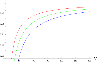
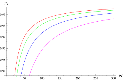
Figure 1: $n_{s}$ versus $\mathcal{N}$ for $\gamma=1$. The left plot is for $g=0.5,~{}n=1.1$ (red), $n=1.5$ (green) and $n=2$ (blue) and right for $g=0.8,~{}n=1.5$ (red), $n=2$ (green), $n=3$ (blue) and $n=5$ (magenta).

The tensor power spectrum is obtained using Eqs.(19), (25) and (30) as

$$\mathcal{P}_{T} = \frac{2\kappa^{2}}{\pi^{2}}(\gamma g)^{2}\left(\frac{\mathcal{N}}{\gamma}+\frac{1-g}{\gamma g}\right)^{\frac{2}{g}(g-1)}.$$

Equations (20) and (26) give the expression for tensor spectrum as

$$n_{T}=2\frac{(g-1)}{\gamma g}\left(\frac{\mathcal{N}}{\gamma}+\frac{1-g}{\gamma g}\right)^{-1}.$$

Using Eqs.(14), (21), (24), (25) and (30), the tensor-scalar ratio is given by

$$r = \left(\frac{144\kappa^{4}(4\pi)^{3}}{\chi_{0}^{3}\pi^{4}}\right)^{\frac{1}{2}}\left(\frac{2C}{3}\right)^{\frac{1}{4}}(384(24)^{n-2}\alpha n(n-1)(g-1))^{\frac{3}{4}}(\gamma g)^{\frac{1}{4}(12n-1)}$$

$$\times \left(\frac{\mathcal{N}}{\gamma}+\frac{1-g}{\gamma g}\right)^{\frac{(12ng-12n-g-2)}{4g}}.$$

In terms of $n_{s}$, the above equation becomes

$$r = \left(\frac{144\kappa^{4}(4\pi)^{3}}{\chi_{0}^{3}\pi^{4}}\right)^{\frac{1}{2}}\left(\frac{2C}{3}\right)^{\frac{1}{4}}(384(24)^{n-2}\alpha n(n-1)(g-1))^{\frac{3}{4}}(\gamma g)^{\frac{1}{4}(12n-1)}$$ (34)

$$\times \left(\frac{12n-12ng+9g-6}{4\gamma g(n_{s}-1)}\right)^{\frac{(12ng-12n-g-2)}{4g}}.$$

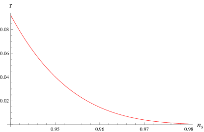
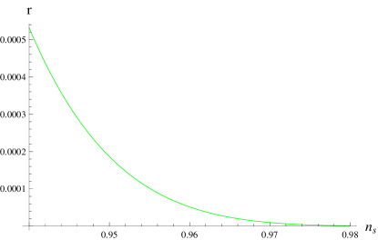
Figure 2: $r$ versus $n_{s}$ for $\gamma=1,~{}g=0.5,~{}\alpha=-1\times 10^{-3},C=70$ and $\chi_{0}\propto C^{\frac{1}{6}}$. The left plot is for $n=1.1$ and right for $n=1.5$.

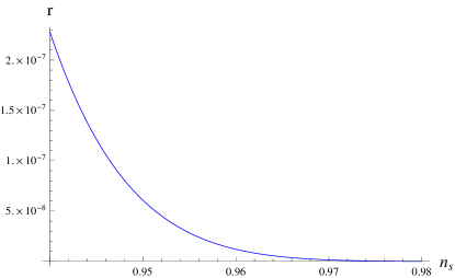
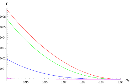
Figure 3: $r$ versus $n_{s}$ for $\gamma=1,~{}\alpha=-1\times 10^{-3},C=70$ and $\chi_{0}\propto C^{\frac{1}{6}}$. The left plot is for $n=2$ with $g=0.5$ and right for $g=0.8,~{}n=1.5$ (red), $n=2$ (green), $n=3$ (blue) and $n=5$ (magenta).

The graphical behavior of $r$ versus $n_{s}$ is given in Figures 2 and 3. The model is compatible with Planck data for the values $n=1.1,~{}1.5$ as shown in Figure 2. The left panel of Figure 3 gives incompatible value of $r$ as it gets very small for $n=2$ and hence can be neglected. In the right plot, $n_{s}$ lies in the region where $r<0.11$ for $n=1.5,~{}2,~{}3$ whereas the observational value of $r$ is inconsistent for $n=5$.

3.2 Case II: $\chi=\chi_{*}\frac{T^{3}}{\varphi^{2}}$

In this case, the scalar field and Hubble parameter are

$$\varphi=\varphi_{0}\exp(\Delta_{2}t^{\frac{3}{8}g-\frac{n}{2}(1-g)+\frac{1}{2}}),\quad H=\gamma g\left(\frac{\ln\varphi-\ln\varphi_{0}}{\Delta_{2}}\right)^{\frac{(g-1)}{\frac{3}{8}g-\frac{n}{2}(1-g)+\frac{1}{2}}},$$ (35)

where $\Delta_{2}=\frac{8(4C\gamma g)^{\frac{3}{8}}}{\chi_{*}^{\frac{1}{2}}(3g-4n(1-g)+4)}[6(384)(24)^{n-2}\alpha n(n-1)(g-1)(\gamma g)^{4n}]^{\frac{1}{8}}$ with $\alpha<0$. The slow-roll parameters lead to

$$\varepsilon = \left(\frac{1-g}{\gamma g}\right)\left(\frac{\ln\varphi-\ln\varphi_{0}}{\Delta_{2}}\right)^{\frac{-g}{\frac{3}{8}g-\frac{n}{2}(1-g)+\frac{1}{2}}},$$ (36)

$$\eta = \left(\frac{2-g}{\gamma g}\right)\left(\frac{\ln\varphi-\ln\varphi_{0}}{\Delta_{2}}\right)^{\frac{-g}{\frac{3}{8}g-\frac{n}{2}(1-g)+\frac{1}{2}}}.$$ (37)

The corresponding radiation density can be described as

$$\rho_{r}=\frac{3}{2}(384)(24)^{n-2}\alpha n(n-1)(\gamma g)^{4n-1}(g-1)\left(\frac{\ln\varphi-\ln\varphi_{0}}{\Delta_{2}}\right)^{\frac{4ng-4n-g}{\frac{3}{8}g-\frac{n}{2}(1-g)+\frac{1}{2}}}.$$

The number of e-folds between $\varphi_{0}$ and $\varphi_{i}$ is given as

$$\mathcal{N}=\gamma\left[\left(\frac{\ln\varphi-\ln\varphi_{0}}{\Delta_{2}}\right)^{\frac{g}{\frac{3}{8}g-\frac{n}{2}(1-g)+\frac{1}{2}}}-\left(\frac{\ln\varphi_{i}-\ln\varphi_{0}}{\Delta_{2}}\right)^{\frac{g}{\frac{3}{8}g-\frac{n}{2}(1-g)+\frac{1}{2}}}\right],$$ (38)

where

$$\varphi_{i}=\varphi_{0}\exp\left[\Delta_{2}\left(\frac{1-g}{\gamma g}\right)^{\frac{\frac{3}{8}g-\frac{n}{2}(1-g)+\frac{1}{2}}{g}}\right].$$

Inserting the value of $\varphi_{i}$ in Eq.(38), we have

$$\varphi=\varphi_{0}\exp\left[\Delta_{2}\left(\frac{\mathcal{N}}{\gamma}+\frac{1-g}{\gamma g}\right)^{\frac{\frac{3}{8}g-\frac{n}{2}(1-g)+\frac{1}{2}}{g}}\right].$$ (39)

The scalar power spectrum and spectral index have the following expressions in terms of $\mathcal{N}$ as

$$\mathcal{P}_{s} = \left(\frac{\chi_{*}^{3}}{36(4\pi)^{3}}\right)^{\frac{1}{2}}\left[\left(\frac{3}{2C}\right)^{11}\left(384(24)^{n-2}\alpha n(n-1)(\gamma g)^{4n+3}(g-1)\right)^{3}\right]^{\frac{1}{8}}$$

$$\times \varphi_{0}^{-3}\exp\left[-3\Delta_{2}\left(\frac{\mathcal{N}}{\gamma}+\frac{1-g}{\gamma g}\right)^{\frac{1}{g}(\frac{3}{8}g-\frac{n}{2}(1-g)+\frac{1}{2})}\right]$$

$$\times \left(\frac{\mathcal{N}}{\gamma}+\frac{1-g}{\gamma g}\right)^{\frac{76ng-76n-23g+20}{8g}},$$

$$n_{s} = 1-\frac{76ng-76n-23g+20}{8\gamma g}\left(\frac{\mathcal{N}}{\gamma}+\frac{1-g}{\gamma g}\right)^{-1}.$$ (40)

Figure 4 represents negative values of $\mathcal{N}$ and hence the required amount of inflation cannot be obtained for variable dissipation factor. Consequently, the observational parameter is not consistent with Planck data.

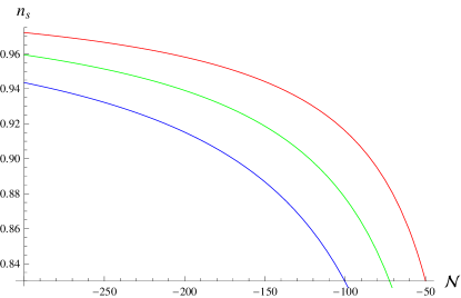
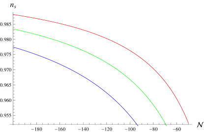
Figure 4: $n_{s}$ versus $\mathcal{N}$ for $\gamma=1$. The left plot is for $g=0.5,~{}n=1.1$ (red), $n=1.5$ (green) and $n=2$ (blue) and right for $g=0.8$.

4 Logamediate Inflation

In this section, we study the dynamics of warm logamediate inflation for the power-law model (22). The logamediate inflation is motivated by applying weak general conditions on the indefinitely expanding cosmological models. For this regime, the scale factor has the form [12]

$$a(t)=a_{0}\exp(\lambda[\ln t]^{h}),\quad\lambda>0,\quad h>1.$$ (41)

For $h=1$, this model is converted to power-law inflation $(a(t)=a_{0}t^{\lambda},~{}\lambda>1)$. The corresponding number of e-folds reads

$$\mathcal{N}=\lambda[(\ln t)^{h}-(\ln t_{i})^{h}].$$ (42)

In the following, we evaluate inflationary parameters for the constant as well as variable dissipation factor.

4.1 Case I: $\chi=\chi_{0}$

The solution for the inflaton is obtained using Eqs.(22) and (41) in (13) as follows

$$\varphi=\varphi_{0}+\Delta_{3}\Omega(t),$$ (43)

where

$$\Delta_{3}=-\left[\frac{6}{\chi_{0}}(-384(24)^{n-2}\alpha n(n-1))\right]^{\frac{1}{2}}(\lambda h)^{2n}\left[-\left(\frac{1}{2}-2n\right)\right]^{-2(h-1)n-1},$$

and $\Omega(t)=\Gamma\left[2(h-1)n+1,-(\frac{1}{2}-2n)\ln t\right]$ is an incomplete gamma function. The Hubble parameter is

$$H=\lambda h\frac{\left[\ln\left(\Omega^{-1}\left(\frac{\varphi-\varphi_{0}}{\Delta_{3}}\right)\right)\right]^{h-1}}{\Omega^{-1}\left(\frac{\varphi-\varphi_{0}}{\Delta_{3}}\right)}.$$ (44)

Using the above equation in Eq.(11), the slow-roll parameters are

$$\varepsilon=\frac{1}{\lambda h}\left[\ln\Omega^{-1}\left(\frac{\varphi-\varphi_{0}}{\Delta_{3}}\right)\right]^{1-h},\quad\eta=\frac{2}{\lambda h}\left[\ln\Omega^{-1}\left(\frac{\varphi-\varphi_{0}}{\Delta_{3}}\right)\right]^{1-h}.$$ (45)

The number of e-folds is

$$\mathcal{N}=\lambda\left[\left(\ln\Omega^{-1}\left(\frac{\varphi-\varphi_{0}}{\Delta_{3}}\right)\right)^{h}-\left(\ln\Omega^{-1}\left(\frac{\varphi_{i}-\varphi_{0}}{\Delta_{3}}\right)\right)^{h}\right].$$

Evaluating the value of $\varphi_{i}$ at $\varepsilon=1$ and inserting in the above equation, it follows that

$$\mathcal{N}=\lambda\left[\left(\ln\Omega^{-1}\left(\frac{\varphi-\varphi_{0}}{\Delta_{3}}\right)\right)^{h}-(\lambda h)^{\frac{h}{1-h}}\right],$$ (46)

which can also be written as

$$\varphi=\varphi_{0}+\Delta_{3}\Omega\left[\exp\left\{\left(\frac{\mathcal{N}}{\lambda}+(\lambda h)^{\frac{h}{1-h}}\right)^{\frac{1}{h}}\right\}\right].$$ (47)

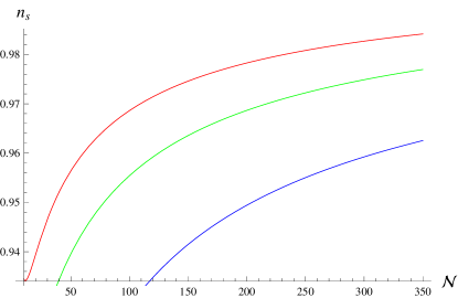
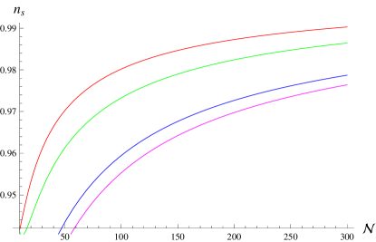
Figure 5: $n_{s}$ versus $\mathcal{N}$. (Left) $\lambda=1,~{}h=3,n=1.5$ (red), $n=2$ (green) and $n=3$ (blue). (Right) $\lambda=0.01,~{}h=5,n=1.5$ (red), $n=2$ (green), $n=3$ (blue) and $n=3.3$ (magenta).

The scalar and tensor power spectra in terms of $\mathcal{N}$ are

$$\mathcal{P}_{s} = \left(\frac{\chi_{0}^{3}}{36(4\pi)^{3}}\right)^{\frac{1}{2}}\left(\frac{3}{2C}\right)^{\frac{1}{4}}[-384(24)^{n-2}\alpha n(n-1)]^{\frac{-3}{4}}(\lambda h)^{\frac{3}{4}(3-4n)}$$

$$\times \left[\exp\left\{\left(\frac{\mathcal{N}}{\lambda}+(\lambda h)^{\frac{h}{1-h}}\right)^{\frac{1}{h}}\right\}\right]^{3n-\frac{3}{2}}\left(\frac{\mathcal{N}}{\lambda}+(\lambda h)^{\frac{h}{1-h}}\right)^{\frac{3}{4h}(h-1)(3-4n)},$$

$$\mathcal{P}_{T} = \frac{2\kappa^{2}}{\pi^{2}}(\lambda h)^{2}\left(\frac{\mathcal{N}}{\lambda}+(\lambda h)^{\frac{h}{1-h}}\right)^{\frac{2}{h}(h-1)}\exp\left[-2\left(\frac{\mathcal{N}}{\lambda}+(\lambda h)^{\frac{h}{1-h}}\right)^{\frac{1}{h}}\right].$$

Equations (17) and (20) lead to the scalar and tensor spectral indices, respectively as

$$n_{s} = 1-\frac{1}{\lambda h}\left(3n-\frac{3}{2}\right)\left(\frac{\mathcal{N}}{\lambda}+(\lambda h)^{\frac{h}{1-h}}\right)^{\frac{1}{h}-1}-\frac{3}{4\lambda h}(h-1)(3-4n)$$ (48)

$$\times \left(\frac{\mathcal{N}}{\lambda}+(\lambda h)^{\frac{h}{1-h}}\right)^{-1},$$

$$n_{T} = -\frac{2}{\lambda h}\left(\frac{\mathcal{N}}{\lambda}+(\lambda h)^{\frac{h}{1-h}}\right)^{\frac{1-h}{h}}.$$

The increasing behavior of $n_{s}$ versus $\mathcal{N}$ is shown in Figure 5. In the left plot, for $n=1.5,~{}2,~{}3$, the corresponding values of $\mathcal{N}$ are $63,~{}125,~{}313$. The number of e-folds $29,~{}47,~{}105$ and $126$ are obtained for $n=1.5,~{}2,~{}3$ and $3.3$ in the right plot. In terms of $\mathcal{N}$, the corresponding tensor-scalar ratio is

$$r = \left(\frac{144\kappa^{4}(4\pi)^{3}}{\chi_{0}^{3}\pi^{4}}\right)^{\frac{1}{2}}[-384(24)^{n-2}\alpha n(n-1)]^{\frac{3}{4}}\left(\frac{2C}{3}\right)^{\frac{1}{4}}(\lambda h)^{3n-\frac{1}{4}}$$

$$\times \exp\left[\left(-3n-\frac{1}{2}\right)\left(\frac{\mathcal{N}}{\lambda}+(\lambda h)^{\frac{h}{1-h}}\right)^{\frac{1}{h}}\right]\left(\frac{\mathcal{N}}{\lambda}+(\lambda h)^{\frac{h}{1-h}}\right)^{\frac{1}{h}(h-1)\left(3n-\frac{1}{4}\right)}.$$

Figure 6 shows the parametric plot of Eqs.(48) and (LABEL:55). The left panel shows that compatible results are obtained for $n=1.5$ and $n=2$ while the observational parameters are in agreement for $n=2$ and $3$ in the right plot.

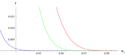
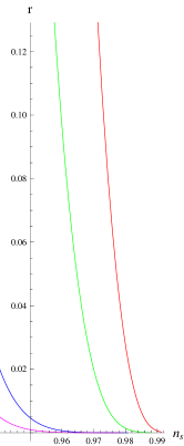
Figure 6: $r$ versus $n_{s}$ for $\alpha=-1\times 10^{-3},~{}C=70,~{}\chi_{0}\propto C^{\frac{1}{6}},~{}n=1.5$ (red), $n=2$ (green) and $n=3$ (blue). The left plot is for $\lambda=1$ with $h=3$ and right for $\lambda=0.01,~{}h=5$ and $n=3.3$ (magenta).

4.2 Case II: $\chi=\chi_{*}\frac{T^{3}}{\varphi^{2}}$

In this case, the scalar field is found to be

$$\varphi=\varphi_{0}\exp(\Delta_{4}\Xi(t)),$$ (50)

where

$$\Delta_{4} = -\left(\frac{6}{\chi_{*}}\right)^{\frac{1}{2}}\left(\frac{2C}{3}\right)^{\frac{3}{8}}[-384(24)^{n-2}\alpha n(n-1)]^{\frac{1}{8}}(\lambda h)^{\frac{1}{8}(4n+3)}$$

$$\times \left(\frac{n-1}{2}\right)^{\frac{-1}{8}(h-1)(4n+3)-1},\quad\alpha<0,$$

and $\Xi(t)=\Gamma\left[\frac{1}{8}(h-1)(4n+3)+1,\frac{1}{2}(n-1)\ln t\right]$ is an incomplete gamma function. The Hubble parameter becomes

$$H=\frac{\lambda h\left[\ln\Xi^{-1}\left(\frac{\ln\varphi-\ln\varphi_{0}}{\Delta_{4}}\right)\right]^{h-1}}{\Xi^{-1}\left(\frac{\ln\varphi-\ln\varphi_{0}}{\Delta_{4}}\right)},$$ (51)

and the corresponding $(\varepsilon,\eta)$ parameters are

$$\varepsilon=\frac{1}{\lambda h}\left[\ln\Xi^{-1}\left(\frac{\ln\varphi-\ln\varphi_{0}}{\Delta_{4}}\right)\right]^{1-h},\quad\eta=\frac{2}{\lambda h}\left[\ln\Xi^{-1}\left(\frac{\ln\varphi-\ln\varphi_{0}}{\Delta_{4}}\right)\right]^{1-h}.$$ (52)

The number of e-folds is given as

$$\mathcal{N} = \lambda\left[\left(\ln\Xi^{-1}\left(\frac{\ln\varphi-\ln\varphi_{0}}{\Delta_{4}}\right)\right)^{h}-\left(\ln\Xi^{-1}\left(\frac{\ln\varphi_{1}-\ln\varphi_{0}}{\Delta_{4}}\right)\right)^{h}\right],$$ (53)

$$= \lambda\left[\left(\ln\Xi^{-1}\left(\frac{\ln\varphi-\ln\varphi_{0}}{\Delta_{4}}\right)\right)^{h}-(\lambda h)^{\frac{h}{1-h}}\right],$$

while the scalar field in terms of $\mathcal{N}$ is expressed as

$$\varphi=\varphi_{0}\exp\left[\Delta_{4}\Xi\left[\exp\left\{\left(\frac{\mathcal{N}}{\lambda}+(\lambda h)^{\frac{h}{1-h}}\right)^{\frac{1}{h}}\right\}\right]\right].$$ (54)

The spectrum parameters $\mathcal{P}_{s}$ and $\mathcal{P}_{T}$ are

$$\mathcal{P}_{s} = \left(\frac{\chi_{*}^{3}}{36(4\pi)^{3}}\right)^{\frac{1}{2}}\left(\frac{3}{2C}\right)^{\frac{11}{8}}[-384(24)^{n-2}\alpha n(n-1)]^{\frac{3}{8}}(\lambda h)^{\frac{3}{8}(4n+3)}\varphi_{0}^{-3}$$

$$\times \exp\left[-3\Delta_{4}\Xi\left(\exp\left\{\left(\frac{\mathcal{N}}{\lambda}+(\lambda h)^{\frac{h}{1-h}}\right)^{\frac{1}{h}}\right\}\right)\right]\exp\left[\frac{-3}{2}(n+1)\right.$$

$$\times \left.\left(\frac{\mathcal{N}}{\lambda}+(\lambda h)^{\frac{h}{1-h}}\right)^{\frac{1}{h}}\right]\left(\frac{\mathcal{N}}{\lambda}+(\lambda h)^{\frac{h}{1-h}}\right)^{\frac{3}{8h}(h-1)(4n+3)},$$

$$\mathcal{P}_{T} = \frac{2\kappa^{2}}{\pi^{2}}(\lambda h)^{2}\left(\frac{\mathcal{N}}{\lambda}+(\lambda h)^{\frac{h}{1-h}}\right)^{\frac{2}{h}(h-1)}\exp\left[-2\left(\frac{\mathcal{N}}{\lambda}+(\lambda h)^{\frac{h}{1-h}}\right)^{\frac{1}{h}}\right].$$

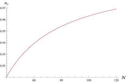
Figure 7: $n_{s}$ versus $\mathcal{N}$ for $\lambda=0.01,~{}h=3,n=3$.

The corresponding spectral indices in terms of $\mathcal{N}$ are as follows

$$n_{s} = 1-\frac{3}{8h\lambda}(h-1)(4n+3)\left(\frac{\mathcal{N}}{\lambda}+(\lambda h)^{\frac{h}{1-h}}\right)^{-1},$$ (55)

$$n_{T} = -\frac{2}{\lambda h}\left(\frac{\mathcal{N}}{\lambda}+(\lambda h)^{\frac{h}{1-h}}\right)^{\frac{1-h}{h}}.$$

Figure 7 yields the increasing behavior of $n_{s}$ with respect to $\mathcal{N}$. The observational value $(n_{s}=0.96)$ corresponds to $\mathcal{N}=94$ which predicts the physical compatibility of the isotropic model. Using Eqs.(14), (22), (41) and (54) in Eq.(21), we get the expression for $r$ as

$$r = \left(\frac{144\kappa^{4}(4\pi)^{3}}{\chi_{*}^{3}\pi^{4}}\right)^{\frac{1}{2}}\left(\frac{2C}{3}\right)^{\frac{11}{8}}[-384(24^{n-2}\alpha n(n-1))]^{\frac{-3}{8}}(\lambda h)^{\frac{1}{8}(-12n+7)}$$

$$\times \varphi_{0}^{3}\exp\left[3\Delta_{4}\Xi\left(\exp\left\{\left(\frac{\mathcal{N}}{\lambda}+(\lambda h)^{\frac{h}{1-h}}\right)^{\frac{1}{h}}\right\}\right)\right]\exp\left[\frac{1}{8}(12n-4)\right.$$

$$\times \left.\left(\frac{\mathcal{N}}{\lambda}+(\lambda h)^{\frac{h}{1-h}}\right)^{\frac{1}{h}}\right]\left(\frac{\mathcal{N}}{\lambda}+(\lambda h)^{\frac{h}{1-h}}\right)^{\frac{1}{8h}(h-1)(-12n+7)},$$

which can also be written in the form of $n_{s}$ as

$$r = \left(\frac{144\kappa^{4}(4\pi)^{3}}{\chi_{*}^{3}\pi^{4}}\right)^{\frac{1}{2}}\left(\frac{2C}{3}\right)^{\frac{11}{8}}[-384(24^{n-2}\alpha n(n-1))]^{\frac{-3}{8}}(\lambda h)^{\frac{1}{8}(-12n+7)}$$ (56)

$$\times \varphi_{0}^{3}\exp\left[3\Delta_{4}\Xi\left(\exp\left\{\left(\frac{3(h-1)(4n+3)}{8\lambda h(1-n_{s})}\right)^{\frac{1}{h}}\right\}\right)\right]\exp\left[\frac{1}{8}(12n-4)\right.$$

$$\times \left.\left(\frac{3(h-1)(4n+3)}{8\lambda h(1-n_{s})}\right)^{\frac{1}{h}}\right]\left(\frac{3(h-1)(4n+3)}{8\lambda h(1-n_{s})}\right)^{\frac{1}{8h}(h-1)(-12n+7)}.$$

The graphical behavior of $r$ versus $n_{s}$ is shown in Figure 8. Three different choices of dissipation factor gives compatible results for $n=3$ with Planck data.

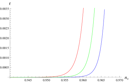
Figure 8: $r$ versus $n_{s}$ for $n=3,~{}\lambda=0.01,~{}h=3,~{}C=70,~{}\varphi_{0}\propto C^{\frac{-1}{12}},~{}\alpha=-1\times 10^{-3},~{}\chi_{*}=0.25$ (red), $1$(green) and $4$(blue).

5 Conclusions

In this paper, we have explored warm inflation for FRW universe model in the background of $f(\mathcal{G})$ gravity. In warm inflation, the interactions between scalar and other fields are taken into account which give the dissipation term. We have formulated the conservation equation, slow-roll parameters $(\varepsilon,\eta)$, scalar and tensor power spectra $(\mathcal{P}_{s},\mathcal{P}_{T})$, spectral indices $(n_{s},n_{T})$ and tensor-scalar ratio using the field equations under the slow-roll approximations.

We have investigated intermediate and logamediate inflationary eras for strong dissipative regime. In each case, we have assumed two specific forms of dissipation factor (a positive constant and a function of scalar field) and a power-law model of $f(\mathcal{G})$ gravity and have evaluated all the above mentioned parameters. The trajectories of $\mathcal{N}$ and $r$ versus $n_{s}$ have been plotted to check the compatibility of the model with observational Planck data in each case. The results are summarized as follows.

• In intermediate regime, for $g=0.5$ and $\gamma=1$, the number of e-folds increases by increasing the values of $n$ while the corresponding $r-n_{s}$ trajectories lead to physical compatible range $1<n<2$. When $g=0.8$, it is found that $n$ lies between 1 and 5 as shown in Figure 3 for constant dissipation factor.

• For the variable dissipation factor in intermediate epoch, the model is inconsistent with observational data.

• In logamediate inflationary era, $n\leq 2$ gives consistent results for $h=3$ and $\lambda=1$. For $h=5$ and $\lambda=0.01$, the physical acceptable range is $2\leq n<3.3$ as shown in Figures 5 and 6.

• In the second case of logamediate era, the effect of dissipation coefficient $\chi_{*}$ is examined for $n=3,~{}\lambda=0.01$ and $h=3$. It is shown in Figure 8 that the results are compatible with observational data for all chosen values of $\chi_{*}$ .

Finally, we conclude that power-law model is consistent with Planck data except for the variable dissipation factor in intermediate inflationary regime.

References

- [1] Perlmutter, S. et al.: Astrophys. J. 483(1997)565; Riess, A.G. et al.: Astron. J. 116(1998)1009; Tegmark, M. et al.: Phys. Rev. D 69(2004)103501.
- [2] Brans, C. and Dicke, R.H.: Phys. Rev. 124(1961)925; Maeda, H.: Class. Quantum Grav. 23(2006)2155; Nojiri, S. and Odintsov, S.D.: Int. J. Geom. Methods Mod. Phys. 04(2007)115.
- [3] Nojiri, S. and Odintsov, S.D.: Phys. Lett. B 631(2005)1.
- [4] Cognola, G., Elizalde, E., Nojiri, S., Odintsov, S.D. and Zerbini, S.: Phys. Rev. D 73(2006)084007.
- [5] De Felice, A. and Tsujikawa, S.: Phys. Rev. D 80(2009)063516.
- [6] Guth, A.H.: Phys. Rev. D 23(1981)347; Albrecht, A. and Steinhardt, P.J.: Phys. Rev. Lett. 48(1982)1220.
- [7] Hawking, S.W.: Phys. Lett. B 115(1982)295; Bardeen, J.M., Steinhardt, P.J., and Turner, M.S.: Phys. Rev. D 28(1983)679.
- [8] Kofman, L., Linde, A. and Starobinsky, A.A.: Phys. Rev. Lett. 73(1994)3195; Khlebnikov, S.Y. and Tkachev, I.I.: Phys. Rev. Lett. 77(1996)219; Bassett, B.A., Tsujikawa, S. and Wands, D.: Rev. Mod. Phys. 78(2006)537.
- [9] Berera, A.: Phys. Rev. Lett. 75(1995)3218; Berera, A.: Phys. Rev. D 55(1997)3346.
- [10] Berera, A.: Nucl. Phys. B 585(2000)666; Hall, L.M.H., Moss, I.G. and Berera, A.: Phys. Rev. D 69(2004)083525.
- [11] Barrow, J.D. and Saich, P.: Phys. Lett. B 249(1990)406; Barrow, J.D.: Phys. Lett. B 235(1990)40.
- [12] Barrow, J.D.: Class. Quantum Grav. 13(1996)2965; Barrow, J.D. and Nunes, N.J.: Phys. Rev. D 76(2007)043501.
- [13] Herrera, R., Olivares, M. and Videla, N.: Phys. Rev. D 88(2013)063535.
- [14] Setare, M.R. and Kamali, V.: Phys. Lett. B 726(2013)56.
- [15] Sharif, M. and Saleem, R.: Eur. Phys. J. C 74(2014)2738.
- [16] Banijamali, A. and Fazlpour, B.: Eur. Phys. J. C 71(2011)1684.
- [17] Bamba, K., Nojiri, S., Odintsov, S.D. and Sáez-Gómez, D.: Phys. Rev. D 90(2014)124061.
- [18] Bamba, K. and Odintsov, S.D.: Symmetry 7(2015)220.
- [19] De Laurentis, M., Paolella, M. and Capozziello, S.: Phys. Rev. D 91(2015)083531.
- [20] Myrzakul, S., Myrzakulov, R. and Sebastiani, L.: Eur. Phys. J. C 75(2015)111.
- [21] Zhang, Y.: J. Cosmol. Astropart. Phys. 03(2009)023; Bastero-Gil, M., Berera, A. and Ramos, R.O.: J. Cosmol. Astropart. Phys. 07(2011)030.
- [22] Moss, I.G. and Xiong, C.: arXiv:hep-ph/0603266; Berera, A., Moss, I.G. and Ramos, R.O.: Rept. Prog. Phys. 72(2009)026901; Bastero-Gil, M., Berera, A. and Ramos, R.O.: J. Cosmol. Astropart. Phys. 09(2011)033; Herrera, R., Videla, N. and Olivares, M.: Phys. Rev. D 90(2014)103502.
- [23] Starobinsky, A.A.: Phys. Lett. B 117(1982)175; Rubakov, V.A., Sazhin, M.V. and Veryaskin, A.V.: Phys. Lett. B 115(1982)189.
- [24] Ade, P.A.R. et al.: Astron. Astrophys. 571(2014)A16.