Pulsar lensing geometry

Abstract

Our analysis of archival VLBI data of PSR 0834+06 revealed that its scintillation properties can be precisely modelled using the inclined sheet model (Pen & Levin, 2014), resulting in two distinct lens planes. These data strongly favour the grazing sheet model over turbulence as the primary source of pulsar scattering. This model can reproduce the parameters of the observed diffractive scintillation with an accuracy at the percent level. Comparison with new VLBI proper motion results in a direct measure of the ionized ISM screen transverse velocity. The results are consistent with ISM velocities local to the PSR 0834+06 sight-line (through the Galaxy). The simple 1-D structure of the lenses opens up the possibility of using interstellar lenses as precision probes for pulsar lens mapping, precision transverse motions in the ISM, and new opportunities for removing scattering to improve pulsar timing. We describe the parameters and observables of this double screen system. While relative screen distances can in principle be accurately determined, a global conformal distance degeneracy exists that allows a rescaling of the absolute distance scale. For PSR B0834+06, we present VLBI astrometry results that provide (for the first time) a direct measurement of the distance of the pulsar. For targets where independent distance measurements are not available, which are the cases for most of the recycled millisecond pulsars that are the targets of precision timing observations, the degeneracy presented in the lens modelling could be broken if the pulsar resides in a binary system.

1 Introduction

Pulsars have long provided a rich source of astrophysical information due to their compact emission and predictable timing. One of the least well constrained parameters for most pulsars is their distance. For some pulsars, timing parallax or VLBI parallax has resulted in direct distance determination. For most pulsars, the distance is a major uncertainty for precision timing interpretations, including mass, moment of inertia (Kramer et al., 2006; Lorimer & Kramer, 2012), and gravitational wave direction (Boyle & Pen, 2012).

Direct VLBI observations of PSR B0834+06 show multiple images lensed by the interstellar plasma. Combining the angular positions and scintillation delays, the authors (Brisken et al., 2010) (hereafter B10) published the derived effective distance (defined in Section 2.1) of $1168\pm 23$ pc for apexes on the main scattering axis. This represents a precise measurement compared to all other attempts to derive distances to this pulsar. This effective distance is a combination of pulsar-screen and earth-screen distances, and does not allow a separate determination of the individual distances. A binary pulsar system would in principle allow a breaking of this degeneracy (Pen & Levin, 2014). One potential limitation is the precision to which the lensing model can be understood.

In this paper, we examine the geometric nature of the lensing screens. In B10, VLBI astrometric mapping directly demonstrated the highly collinear nature of a single dominant lensing structure. First hints of single plane collinear dominated structure had been realized in Stinebring et al. (2001). While the nature of these structures is already mysterious, for this pulsar, in particular, the puzzle is compounded by an offset group of lenses whose radiation arrive delayed by 1 ms relative to the bulk of the pulsar flux. The mysterious nature of lensing questions any conclusions drawn from scintillometry as a quantitative tool (Pen et al., 2014).

Using archival data we demonstrate in this paper that the lensing screen consists of nearly parallel linear refractive structures, in two screens. The precise model confirms the one dimensional nature of the scattering geometry, and thus the small number of parameters that quantify the lensing screen.

The paper is structured as follows. Section 2 overviews the inclined sheet lensing model, and its application to data. Section 3 presents new VLBI proper motion and distance measurements to this pulsar. Section 4 describes the interpretation of the lensing geometry and possible improvements on the observation. We conclude in Section 5.

2 Lensing

In this section, we map the archival data of PSR 0834+06 onto the grazing incidence sheet model. The folded sheet model is qualitatively analogous to the reflection of a light across a lake as seen from the opposite shore. In the absence of waves, exactly one image forms at the point where the angle of incidence is equal to the angle of reflection. In the presence of waves, one generically sees a line of images above and below the unperturbed image. The grazing angle geometry simplifies the lensing geometry, effectively reducing it from a two dimensional problem to one dimension. The statistics of such reflections is sometimes called glitter, and has many solvable properties (Longuet-Higgins, 1960). This is illustrated in Fig. 1.

Figure 1: Reflection of lights on surface waves. At grazing angle, each wave crest results in an apparent image, causing a linear streak of images centred on the unperturbed image location. For example, the red light streak would consist of a single image at its center in the absence of waves. The inclined sheet model for pulsar scintillation is analogous, with reflection replaced by refraction. Image copyright Kaitlyn McLachlan, licensed through shutterstock.com image ID 45186139.

A similar effect occurs when the observer is below the surface. Two major distinctions arise: 1. the waves can deform the surface to create caustics in projection. Near caustics, Snell’s law can lead to highly amplified refraction angles(Goldreich & Sridhar, 2006). 2. due to the odd image theorem, each caustic leads to two images. In an astrophysical context, the surface could be related to magnetic reconnection sheets (Braithwaite, 2015), which have finite widths to regularize these singularities. Diffusive structures have Gaussian profiles, which were analysed in Pen & King (2012). The lensing details differ for convergent (under-dense) vs divergent (over-dense) lenses, first considered by Clegg et al. (1998).

The typical interstellar electron density $\sim 0.02$ cm^-3 is insufficient to deflect radio waves by the observed $\sim$ mas bending angles. At grazing incidence, Snell’s law results in an enhanced bending angle, which formally diverges. Magnetic discontinuities generically allow transverse surface waves, whose restoring force is the difference in Alfvén speed on the two sides of the discontinuity. This completes the analogy to waves on a lake: for sufficiently inclined sheets the waves will appear to fold back onto themselves in projection on the sky. At each fold caustic, Snell’s law diverges, leading to enhanced refractive lensing. The divergence is cut off by the finite width of the sheet. The generic consequence is a series of collinear images. Each projected fold of the wave results in two density caustics. Each density caustic leads to two geometric lensing images, for a total of 4 images for each wave inflection. The two geometric images in each caustic are separated by the characteristic width of the sheet. If this is smaller than the Fresnel scale, the two images become effectively indistinguishable. The geometry of the inclined refractive lens is shown in Fig. 2.

Figure 2: Refractive lensing geometry (reproduced from Pen & Levin (2014) fig. 1). The pulsar is on the right, observer on the left. Each fold of the sheet leads to a divergent projected density, resulting in a lensed image as indicated by the dotted line. See text for details.

A large number of sheets might intersect the line of sight to any pulsar. Only those sufficiently inclined would lead to caustic formation. Empirically, some pulsars show scattering that appears to be dominated by a single sheet, leading to the prominent inverted arclets in the secondary spectrum of the scintillations (Stinebring et al., 2001).

2.1 Archival data of B0834+06

Our analysis is based on the apex data selected from the secondary spectrum of pulsar B0834+06 in B10, which was observed as part of a 300 MHz global VLBI project on 2005 November 12, with the GBT (GB), Arecibo (AR), Lovell and Westerbork (WB) telescopes. The GB-AR and AR-WB baselines are close to orthogonal and of comparable lengths, resulting in relatively isotropic astrometric positions. Information from each identified apex includes delay $\tau$, delay rate (differential frequency $f_{\rm D}$), relative Right Ascension, $\Delta\alpha$, and relative declination, $\Delta\delta$. Data of each apex are collected from four dual circular polarization $8$ MHz wide sub-bands spanning the frequency range $310.5$–$342.5$ MHz. As described in B10, the inverse parabolic arclets were fitted to positions of their apexes, resulting in a catalogue of apexes in each sub-band, each with delay and differential frequency. In this work, we first combine the apexes across sub-bands, resulting in a single set of images. We focus on the southern group with negative differential frequency: this grouping appears as a likely candidate for a double-lensing screen. However, two groups (with negative differential frequency) appear distinct in both the VLBI angular positions and the secondary spectra. We divide the apex data with negative $f_{\rm D}$ into two groups: in one group, time delays range from $0.1$ ms to $0.4$ ms, which we call the $0.4$ ms group; and in the other group, time delay at about $1$ ms, which we call the $1$ ms group. In summary, the $0.4$ ms group contains $10$ apexes in the first two sub-bands, and $14$ apexes in the last two sub-bands; the $1$ ms group, contains $5$, $6$, $5$ and $4$ apexes in the four sub-bands subsequently, with center frequency of each band $f_{\rm band}=314.5,322.5,330.5$ and $338.5$ MHz. The apex positions in the secondary spectrum are shown in Fig. 3.

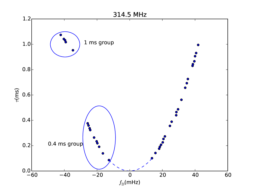
Figure 3: Distribution of the apex positions in the sub-band centred at 314.5 MHz. The apexes that belong to the 1 and 0.4 ms groups are marked.

We select the equivalent apexes from four sub-bands. To match the same apexes in different sub-bands, we scale the differential frequency in different sub-bands to $322.5$ MHz, by $f_{\rm D}(322.5/f_{\rm band})$ MHz. A total of $9$ apexes from the $0.4$ ms group and $5$ apexes from the $1$ ms group, were mapped. This results in an estimation for the mean referenced frequency $f=322.5$ MHz and a standard deviation among the sub-bands, listed in Table 1. The $f_{\rm D}$, $\tau$, $\Delta\alpha$ and $\Delta\delta$ are the mean values of $n$ sub-bands ($n=3$ for points 4 to 6 and points $1^{\prime}$, $2^{\prime}$ and $4^{\prime}$, while 4 for the remainder of the points), listed in Table 1.

label	$\theta_{\parallel}$(mas)	$f_{\rm D}$(mHz)	$\tau$(ms)	$\Delta\alpha$(mas)	$\Delta\delta$(mas)	$t_{0}$(day)
1	$-17.22$	$-26.1(4)$	0.3743(6)	6.2	$-11.9$	$-107$
2	$-16.36$	$-24.9(4)$	0.3378(3)	8.0(4)	$-14.5(8)$	$-101$
3	$-16.08$	$-24.6(4)$	0.327(3)	7.2(6)	$-13.9(4)$	$-99.0$
4	$-14.45$	$-22.3(5)$	0.2633(3)	6.1(4)	$-13.1(7)$	$-88.1$
5	$-13.68$	$-21.6(6)$	0.236(2)	5.1(4)	$-12.7(5)$	$-83.3$
6	$-13.27$	$-20.4(5)$	0.222(3)	5.8(4)	$-11.8(1)$	$-81.4$
7	$-12.21$	$-18.9(2)$	0.188(2)	5.5(6)	$-10.8(6)$	$-74.2$
8	$-10.58$	$-16.8(3)$	0.1412(9)	3.9(6)	$-10.0(4)$	$-62.8$
9	$-8.18$	$-12.9(2)$	0.0845(5)	2.8(3)	$-8.6(4)$	$-48.7$
1’	$\cdots$	$-43.1(4)$	1.066(5)	$-8(3)$	$-24(2)$	$-185$
2’	$\cdots$	$-41.3(5)$	1.037(3)	$-14(1)$	$-23(3)$	$-188$
3’	$\cdots$	$-40.2(6)$	1.005(8)	$-14(1)$	$-22.3(5)$	$-187$
4’	$\cdots$	$-38.3(6)$	0.9763(9)	$-14(1)$	$-20.6(3)$	$-190$
5’	$\cdots$	$-35.1(5)$	0.950(2)	$-15(1)$	$-21(1)$	$-202$

Table 1: $0.4$ ms and $1$ ms reduced apex data. We list the $0.4$ ms group data in the upper part of the table, while the $1$ ms group lie in the lower part of the table. Observation data include the differential frequency $f_{\rm D}$, time delay $\tau$ ($\tau_{1}$ for $0.4$ ms group and $\tau_{2}$ for $1$ ms group); $\Delta\alpha$ and $\Delta\delta$ are from the VLBI measurement (there is only one matched position for point 1, thus no error). $t_{0}$ is the time at constant velocity for an apex to intersect the origin at constant speed along the main scattering parabola. More details in Section 2.1 and Section 2.2.2.

We estimate the error of time delay $\tau$, differential frequency $f_{\rm D}$, $\Delta\alpha$ and $\Delta\delta$ listed in Table 1 from their band-to-band variance:

$$\sigma^{2}_{\rm\tau,f_{\rm D},\Delta\alpha,\Delta\delta}=\frac{1}{n}\sum^{n}_{i=1}\frac{(x_{i}-\bar{x})^{2}}{n-1},$$ (1)

and $n$ is the number of sub-bands. The outer $1/n$ accounts for the expected variance of a mean of $n$ numbers.

2.2 One-lens model

2.2.1 Distance to the lenses

In the absence of a lens model, the fringe rate, delay and angular position cannot be uniquely related. To interpret the data, we adopt the lensing model of Pen & Levin (2014). In this model, the lensing is due to projected fold caustics of a thin sheet closely aligned to the line of sight. We will list the parameters in this lens model in Table 2.

Table 2: Parameters for double-lens model

$D_{1\rm e}$	Effective Distance of $0.4$ group data
$D_{2\rm e}$	Effective Distance of $1$ ms group data
$D_{1}$	Distance of lens 1
$D_{2}$	Distance of lens 2
$\gamma$	Scattering axis angle of $0.4$ ms groupa
$\phi$	Angle of the velocity of the pulsara
$\theta$	Angular offset of the object

• The angle is measured relative to the longitude and east is the positive direction.

We define the effective distance $D_{\rm e}$ as

$$D_{\rm e}\equiv\frac{2c\tau}{\theta^{2}}.$$ (2)

The differential frequency is related to the rate of change of delay as $f_{\rm D}=-f\frac{\rm d\tau}{\operatorname{d\!}t}$. In general, $D_{\rm e}={D_{\rm p}D_{\rm s}}/({D_{\rm p}-D_{\rm s}})$ for a screen at $D_{\rm s}$. The effective distance corresponds to the pulsar distance $D_{\rm p}$, if the screen is exactly halfway. Fig. 4 shows two sets of $D_{\rm p}$ and $D_{\rm s}$ with common $D_{\rm e}$.

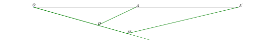
Figure 4: A single refracted light path showing the distance degeneracy. The primed and un-primed geometries result in the same observables: delay $\tau$ and angular offset $\theta$. $O$ denotes the observer; $A$ and $A^{\prime}$ denote the positions of the pulsar; $D$ and $D^{\prime}$ denote the positions of the refracted images on the interstellar medium. The un-primed geometry corresponds to a pulsar distance $D_{\rm p}=|AO|=620$ pc, while the primed geometry has the same $D_{\rm e}$ but twice the $D_{\rm p}.$

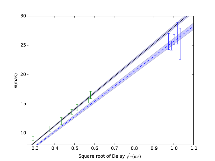
Figure 5: ${\theta}$ vs ${\sqrt{\tau}}$. Two separate lines through the origin were fitted to the points sampled among the $0.4$ ms group and $1$ ms group. The solid line is the fitted line of the $0.4$ ms positions, where $D_{1\rm e}=1044\pm 22$ pc. The dashed line is the fitted line of the $1$ ms position, where $D_{2\rm e}=1252\pm 49$ pc.

When estimating the angular offset of each apex, we subtract the expected noise bias: ${\theta}^{2}=({\Delta\alpha}\cos(\delta))^{2}+({\Delta\delta})^{2}-\sigma^{2}_{\Delta\alpha}-\sigma^{2}_{\Delta\delta}$. We plot the $\theta$ vs square root of $\tau$ in Fig. 5. A least-square fit to the distance results in $D_{1{\rm e}}=1044\pm 22$ pc for the $0.4$ ms group, which we call lens 1 (point 1 is excluded since VLBI astrometry was only known for one sub-band, thus we cannot obtain the variance nor weighted mean for that point), and $D_{2{\rm e}}=1252\pm 49$ pc for the $1$ ms group, hereafter lens 2. The errors, and uncertainties on the error, preclude a definitive interpretation of the apparent difference in distance. However, at face value, this indicates that lens 2 is closer to the pulsar, and we will use this as a basis for the model in this paper. The distances are slightly different from those derived in B10, which is partly due to a different subset of arclets analysed. We discuss consequences of alternate interpretations in Section 2.4. The pulsar distance was directly measured using VLBI parallax to be $D_{\rm p}=620\pm 60$ pc, described in more detail in Section 3. We take $D_{1{\rm e}}=1044$ pc, and the distance of lens 1 $D_{1}$, where $0.4$ ms group scintillation points are refracted, as $389$ pc. Similarly, for $1$ ms apexes, the distance of lens 2 is taken as $D_{2}=415$ pc, slightly closer to the pulsar.

For the 0.4 ms group, we adopt the geometry from B10, assigning these points along line $AD$ as shown in Fig. 6 based solely on their delay, which is the best measured observable. The line $AD$ is taken as a fixed angle of $\gamma=-25\degree.2$ east north. We use this axis to define ${\parallel}$ direction and define ${\bot}$ by a $90\degree$ direction clockwise rotation.

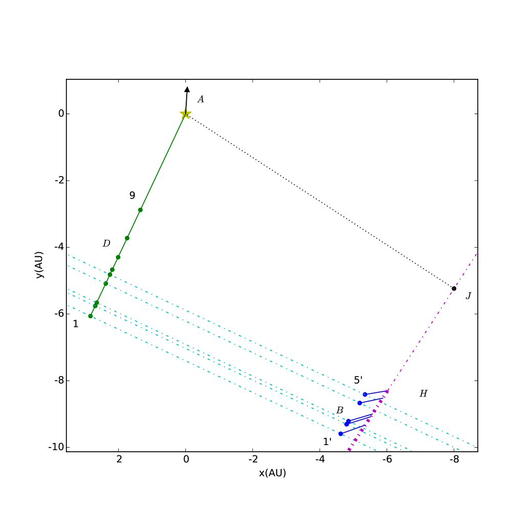
Figure 6: Positions of $0.4$ ms and $1$ ms group data in the one-lens model and double-lens model. The axes represent the relative transverse distances to the un-refracted pulsar in Right Ascension (calculated by $x=\Delta\alpha\cos(\delta)D_{i}$ with $D_{i}$ represent the distance of the object to the observer: for point $A$, $D_{i}=D_{\rm p}$; for points $H$ and $J$, $D_{i}=D_{2}$; for points $B$ and $D$, $D_{i}=D_{1}$.) and declination (calculated by $y=\Delta\delta D_{i}$) directions, on a 2D plane that is transverse to the line of sight. On the left side, the points marked with letter $D$ labelled from 1 to 9, are the derived positions from the time delays of $0.4$ ms group in the one-lens model. At a distance $389$ pc from the observer, the green solid line demarcates the scattering axis for the $0.4$ ms apexes positions, with an angle $\gamma=-25\degree.2$ east of north. The points on the right side mark the first and second refraction points in double-lens model. The unobservable points denoted by the letter $H$, are the calculated positions on lens 2 from the 1 ms group; the observed apparent positions denoted by the letter $B$, are the second refraction on lens 1. They are connected by short solid lines. The long dash dotted line passing through $J$ is the inferred geometry of the second lens. Its thicker portion has formed a full caustic, while the thinner portion are sub critical. The dash dotted lines, constructed perpendicular to the $AD$ scattering axis, denote the caustics of lens 1. The dotted line on the top right is perpendicular to the magenta dash dotted line, intersecting at $J$. The relative model pulsar-screen velocity is $185.3$ km $\rm s^{-1}$, with an angle $\phi=-3\degree.7$ east of north, is marked with an arrow from the star, at point $A$, at the top of the figure.

2.2.2 Discussion of one-lens model

The $0.4$ ms group lens solution appears consistent with the premise of the inclined sheet lensing model (Pen & Levin, 2014), which predicts collinear positions of lensing images. The time in the last column of Table 1, which we denote as $t_{0}=-2{\tau}f/{f_{\rm D}}$, corresponds to the time required for the arclet to drift in the secondary spectrum through a delay of zero.

The collinearity can be considered a post-diction of this model. The precise positions of each image are random, and with 9 images no precision test is possible. The predictive power of the sheet model becomes clear in the presence of a second, off-axis screen, which will be discussed below.

2.3 Double-lens model

The apparent offset of the $1$ ms group can be explained by a second lens screen. The small number of apexes at $1$ ms suggests that the second lens screen involves a single caustic at a different distance. One expects each lens to re-image the full set of first scatterings, resulting in a number of apparent images equal to the product of number of lenses in each screen. In the primary lens system, the inclination appears such that typical waves form caustics. For the sake of discussion, we consider an inclination angle for lens 1 $\iota_{1}=0.1^{o}$, and a typical slope of waves $\sigma_{\iota}=\iota_{1}$. Each wave of gradient larger than 1-$\sigma$ will form a caustic in projection. The number of sheets at shallower inclination increases as the square of this small angle. A 3 times less-inclined $\iota_{2}=0.3^{o}$ sheet occurs 9 times as often. For the same amplitude waves on this second surface, they only form caustics for 3-$\sigma$ waves, which occur two hundred times less often. Thus, one expects such sheets to only form isolated caustics, which we expect to see occasionally. Three free parameters describe a second caustic: distance, angle, and angular separation. We fix the distances from the effective VLBI distance ($D_{1}$ and $D_{2}$), and fit the angular separations and angles with the 5 delays of the $1$ ms group.

2.3.1 Solving the double-lens model

Apexes 1’–5’ share a similar 1 ms time delay, suggesting they are lensed by a common structure. We denote the position of the pulsar point as point $A$, the positions of the lensed image on lens 2 as point $H$, positions of the lensed image on lens 1 as point $B$, position of the observer as point $O$, and the nearest point on lens 2 to the pulsar as point $J$. The lines $AJ\perp HJ$ intersect at point $J$, $HF\perp BD$ intersect at the point $F$, and $BG\perp HJ$ intersect at the point $G$.

A 3D schematic of two plane lensing by linear caustics is shown in Fig. 7.

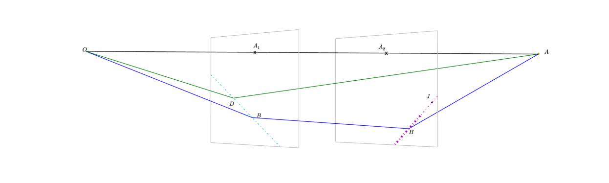
Figure 7: A 3D schematic of light path when light is doubly-refracted. Two planes from left to right are the plane of lens 1, and the plane of lens 2. The dash dotted lines represent the projected line-like fold caustics. Light goes from $A$ (pulsar) to the first refracted point $H$ on lens 2 (line $HJ$, magenta dash dotted line), and then the second refracted point $D$, the image we observe, on lens 1 (line $BD$, cyan dash dotted line), and finally the observer $O$. Dash dotted lines show the light path of singly-deflected light path ($A-D-O$). The crosses ($A_{1}$ on plane 1, and $A_{2}$ on plane 2) denote intersection of the un-deflected light through the lensing sheet. $D$ and $J$ are the closest point of the lens caustic to the un-deflected path, which are the loci of single deflection images. Thus, $A_{2}J\bot HJ$, and $A_{1}D\bot BD$. The thick line on plane 2 indicates the real caustic, while the thin continuation indicates the extrapolated continuation beyond the cusp/swallowtail.

First, we calculate the position of $J$. We estimate the distance of $J$ from the $1$ ms $\theta$–$\sqrt{\tau}$ relation (see Fig. 5). We determine the position of $J$ by matching the time delays of point 4’ and point 1’, which is marked in Fig. 6. The long dash dotted line on the right side of Fig. 6 denotes the inferred geometry of lens 2, and by construction vertical to $AJ$.

The second step is to find the matched pairs of those two lenses. By inspection, we found that the 5 furthest points in $0.4$ ms group match naturally to the double-lens images. These five matched lines are marked with cyan dash dotted lines in Fig. 6 and their values are listed in the second column in Table 3.

label	$\theta_{\parallel}$ (mas)	$\tau_{2}$(ms)	$\sigma_{\rm\tau}$(ms)	$\tau_{\rm M}$(ms)	$f_{\rm D}$(mHz)	$\sigma_{f}$(mHz)	$f_{\rm M}$(mHz)	$t_{1}$(day)
1’	$-17.22$	1.0663	0.0050	1.0663*	$-43.08$	0.84	$-42.26$	$-78$
2’	$-16.36$	1.0370	0.0059	1.0362	$-41.27$	0.88	$-41.04$	$-73$
3’	$-16.08$	1.005	0.011	1.027	$-40.17$	0.87	$-40.64$	$-72$
4’	$-14.45$	0.9763	0.00088	0.9763*	$-38.31$	0.64	$-38.31\dagger$	$-63$
5’	$-13.68$	0.9495	0.0094	0.9550	$-35.06$	0.78	$-37.21$	$-59$

Table 3: Comparison of time delay $\tau$ and the differential frequency $f_{\rm D}$ of the observation and the model fitting result in the double-lens model. $\theta_{\parallel}$ denotes the angular offsets of the corresponding images at lens 1. The values with star symbols on them are the points that we use to calculate the position of $J$ and the point with a $\dagger$ symbol is the point that we use to calculate the transverse velocity of the pulsar $v_{\bot}$. They agree with data by construction. The last column, $t_{1}$ is the time the lensed image on lens 2 takes to move from point $H$ to point $J$, which is also defined in Section 2.3.3.

They are the located at a distance $389$ pc away from us. Here we define three distances:

$$D_{\rm p2} =620~{}{\rm pc}-415~{}{\rm pc}=205~{}{\rm pc},$$ (3)

$$D_{21} =415~{}{\rm pc}-389~{}{\rm pc}=26~{}{\rm pc},$$

where $D_{\rm p2}$ is the distance from the pulsar to lens 2, and $D_{21}$ is the distance from lens 2 to lens 1.

Fig. 8 and Fig. 9 are examples of how light is refracted on the first lens plane and the second lens plane. We specifically choose the point with $\theta_{\parallel}=-17.22$ mas, which refer point 1’ on lens 1 as an example. Equality of the velocity of the photon parallel to the lens plane before and after refraction implies the relation:

$$\frac{JH}{D_{\rm p2}} =\frac{HG}{D_{21}},$$ (4)

$$\frac{FB}{D_{21}} =\frac{BD}{D_{1}}.$$

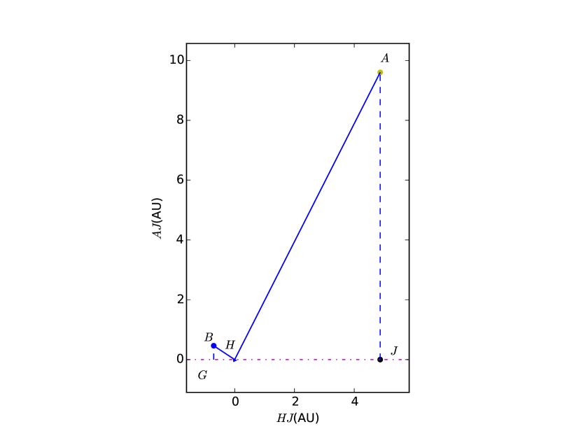
Figure 8: Refraction on lens 2. $A$ is the position of the pulsar. $H$ is the lensed image on lens 2. $B$ is the lensed image on lens 1. $AJ\bot HJ$ and $BG\bot HJ$. We illustrate the scenario for point 1’.

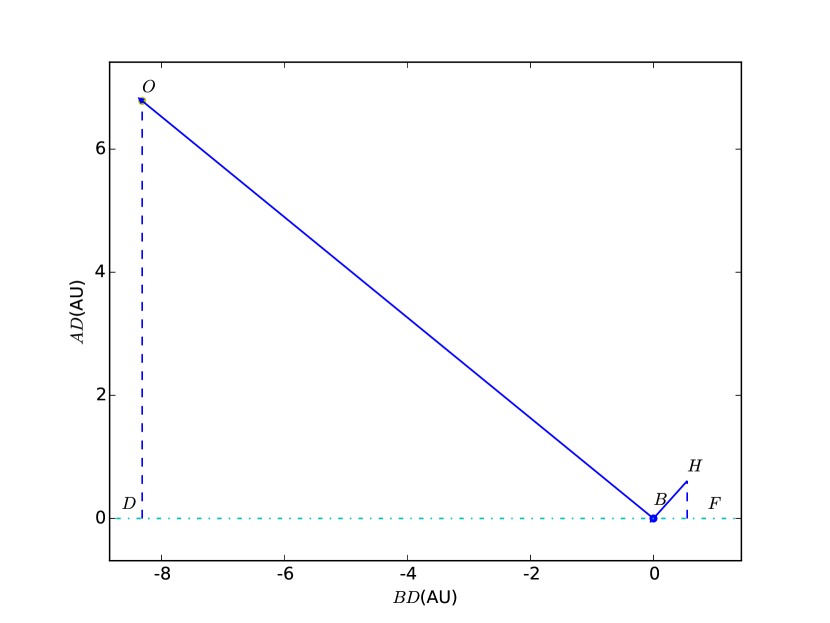
Figure 9: Refraction on lens 1. $H$ is the lensed image on lens 2. $B$ is the lensed image on lens 1. $O$ is the position of the observer. $HF\bot DF$ and $OD\bot HJ$. As in the previous figure, we illustrate the scenario for point 1’.

We plot the solved positions in Fig. 6, and list respective time delays and differential frequencies in Table 3. We take the error of the time delay $\tau$ in the double-lens model as

$$(\frac{\sigma_{\tau_{i}}}{\tau_{2i}})^{2}=(\frac{\sigma_{\tau 1i}}{\tau_{1i}})^{2}+(\frac{\sigma_{\tau 2i}}{\tau_{2i}})^{2}+(\frac{\sigma_{\tau 2j}}{\tau_{2j}})^{2},$$ (5)

where $\tau_{1}$ and $\sigma_{\tau 1}$ represent the time delay and its error from the $0.4$ ms group on lens $1$, and $\tau_{2}$ and $\sigma_{\tau 2}$ represent the time delay and its error from the $1$ ms group on lens 2. And $\tau_{2j}$ is the $\tau_{2}$ for the nearest reference point in Table 3 with error $\sigma_{\tau 2j}$. Specifically, for point $i=5^{\prime}$ and $3^{\prime}$, $j=4^{\prime}$ is the nearest reference point; while for point $i=2^{\prime}$, $j=1^{\prime}$ is the nearest reference point. The reference points are marked with star symbols in the fifth column in Table 3.

For the error of differential frequency $f_{\rm D}$, we add the error of the reference point (point 4’) to the error of each other measured point:

$$(\frac{\sigma_{f_{i}}}{f_{{\rm D}i}})^{2}=(\frac{\sigma_{f_{{\rm D}i}}}{f_{{\rm D}i}})^{2}+(\frac{\sigma_{f_{{\rm D}4^{\prime}}}}{f_{{\rm D}4^{\prime}}})^{2}$$ (6)

where $f_{{\rm D}4^{\prime}}$ and $\sigma_{f_{{\rm D}4^{\prime}}}$ are the differential frequency and we list its error of the point in the fourth row in Table 3.

2.3.2 Comparing with observations

In order to compare $\tau$, we calculate model time delays $\tau_{\rm M}$ for these five points, and list the results in Table 3. For points 4’ and 1’, they fit by construction since we use these to calculate the position of $J$; for the remaining three points, all of the results are within 3-$\sigma$ of the observed time delays.

To compare differential frequency $f_{\rm D}$, we need to calculate the velocity of the pulsar and the velocity of the lens. We take the lenses to be static, and solve the velocity of the pulsar relative to the lens (in geocentric coordinates). The pulsar has two velocity components, and the two 1-D lenses effectively determine one component each. For $v_{\parallel}$, we derive the velocity $172.4\pm 2.4$ km $\rm s^{-1}$, which is $58.7$ mas/yr in a geocentric system, from $f_{\rm D}$ of point $1$ in $0.4$ ms group. The direct observable is the time to crossing of each caustic, denoted $t_{0}$ in Table 1.

To calculate $v_{\bot}$, we choose the point 4’, which has the smallest errorbar of differential frequency. This gives a value of $67.9\pm 2.8$ km $\rm s^{-1}$ for $v_{\perp}$, which is $21.4$ mas/yr in geocentric system, with an angle $\phi=-3\degree.7\pm 0\degree.8$ west of north. This represents the pulsar-screen velocity relative to the Earth. We can further transform this into the local standard of rest (LSR) frame to interpret the velocities in a Galactic context. The model derived and observed velocities (heliocentric and LSR) are listed in Table 4. The direction of the model velocity is marked on the top of the star in Fig. 6.

Parameter	$\mu_{\alpha*}$(mas yr-1)	$\mu_{\delta}$(mas yr-1)	$\mu_{l*}$(mas yr-1)	$\mu_{b}$ (mas yr-1)	$v_{l*}$ (km $\rm s^{-1}$)	$v_{b}$ (km $\rm s^{-1}$)
model pulsar-screen velocity	$-5.30\pm 1.11$	$61.97\pm 1.11$	$-56.45$	22.23	$\cdots$	$\cdots$
VLBI pulsar proper motion	$2.16\pm 0.19$	$51.64\pm 0.13$	$-46.69$	28.02	-137.24	82.34
Screen motion	$\cdots$	$\cdots$	9.76	5.79	18.00	10.68

Table 4: Summary of velocities in double-lens model. The velocities listed in equatorial coordinates are the relative velocity in heliocentric system, while the velocities in Galactic coordinates are the relative velocities in LSR (Local Standard of Rest). $\mu_{\alpha*}=\Delta\alpha\cos(\delta)/t$ and $\mu_{l*}=\Delta l\cos(b)/t$, for we moved the center position from $(\Delta\alpha,\Delta\delta)$ or $(l,b)$ to (0,0). $v_{l*}$ and $v_{b}$ are the linear velocities relative to the LSR. The screen is only moving slowly ($\sim 21$ km $\rm s^{-1}$). Ellipses reflect the unobserved and frame dependent parameters.

With this velocity of the pulsar, we calculate the model differential frequency $f_{\rm M}$ of points 5’,3’,2’ and 1’. Results are listed in Table 3. The calculated results all lie within the 3-$\sigma$ error intervals of the observed data.

The reduced ${\chi}^{2}$ for time delay $\tau$ is $1.5$ for $3$ degrees of freedom and $2.2$ for $f_{\rm D}$ for $4$ degrees of freedom. This is consistent with the model.

Within this lensing model, we can test if the caustics are parallel. Using the lag error range of double-lensed point 4 (the best constrained), we find a 1-$\sigma$ allowed angle of 0.4 degrees from parallel with the whole lensing system. This lends support to the hypothesis of a highly inclined sheet, probably aligned to better than 1 per cent.

2.3.3 Discussion of double-lens model

For the $1$ ms group, lens 2 only images a subset of the lens 1 images. This could happen if lens 1 screen is just under the critical inclination angle, such that only 3-$\sigma$ waves lead to a fold caustic. If the lens 2 was at a critical angle, the chance of encountering a somewhat less inclined system is of order unity. More surprising is the absence of a single-refracted image of the pulsar, which is expected at position $J$. This could happen if the maximum refraction angle is just below critical, such that only rays on the appropriately aligned double refraction can form images. We plot the refraction angle $\beta$ in the direction that is transverse to the first lens plane in Fig. 10. The fractional bandwidth of the data is about 10 per cent, making it unlikely that single lens image $J$ would not be seen due to the larger required refraction angle. Instead, we speculate that the fold caustic terminates near double-lensed image 5’, and thus only intersections with the closer lens plane caustic south of image 5’ are doubly-lensed.

This is a generic outcome of a swallowtail catastrophe (Arnold, 1990). In this picture, the sheet just starts folding near point 5’. North of point 5’, no fold appears in projection. Far south of point 5’, a full fold exhibits two caustics emanating from the fold cusp. Near the cusp the magnification is the superposition of two caustics, leading to enhanced lensing and higher likelihood of being observed.

We denote $t_{1}$ the time for the lensed image on lens 2 to move from point $H$ to point $J$. From our calculation, we predict that on 2005 September 14, which is 59 days before the observation, the lensed image would have appeared overlayed on point $H_{5}$; and on 2005 August 26, which is 78 days before the observation, the lensed image would have appeared overlayed on point $H_{1}$. The model predicts the presence of a singly-lensed image refracted at these points, in addition to the doubly-lensed images.

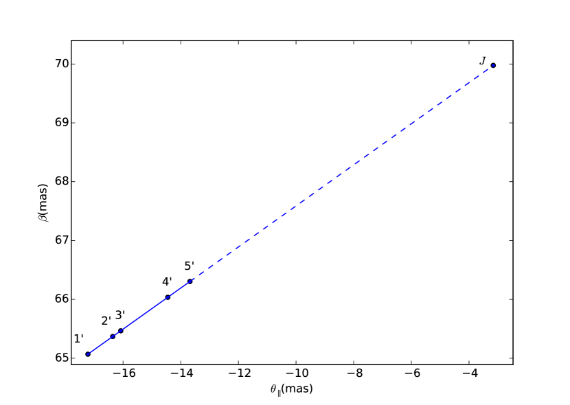
Figure 10: Deflection angle $\beta=\pi-\angle AHB$ on lens 2. Point $J$ denotes the expected position to form a single refraction image, which was not observed. The small change in angle relative to the observed images precludes a finite refraction cut-off, since the data spans 10 per cent bandwidth, with a 20 per cent change in refractive strength. We propose a swallowtail caustic as the likely origin for the termination of the second lens sheet.

The generic flux of a lensed image is the ratio of the lens transverse size to maximum impact parameter (Pen & King, 2012). Near the caustic, the lensed flux can become very high. The 1 ms group is about a factor of 4 fainter than the 0.4 ms group. The high flux of the second caustic suggests it to be relatively wide, perhaps a fraction of an AU. Due to the odd image theorem, one generically expects two distinct set of double lensed arcs. We only see one (generically the outer one), which places an upper bound on the brightness of the inner image. In a divergent lens(Clegg et al., 1998), the inner image is generically much fainter, so perhaps not surprising. For a convergent Gaussian lens, the two images are of similar brightness, but a more cuspy profile will also result in a faint inner image. In gravitational lensing, the odd image theorem is rarely seem to hold, generally thought to be due to one lens being very faint.

One can try to estimate the chance of accidental agreement between model and data. We show the data visually in Fig. 11.

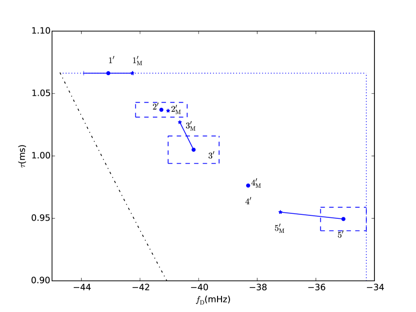
Figure 11: Model comparison. Points with subscripts are derived from the double-lens model, see Table 3. Rectangles mark the 1-$\sigma$ error region. Points 1’ (only for $\tau$) and 4’ were used to fit the model, and thus do not have an error region. The rectangles cover $10^{-3}$ of the area in the dotted region bounded by the parabolic arc and the data points. We interpret this precise agreement between model and data is unlikely to be a random coincidence.

To estimate where points might lie accidentally, we conservatively compare the area of the error regions to the area bounded by the parabola and the data points, as shown by dotted lines. This results in about 10^-3, suggesting that the model is unlikely to be an accidental fit.

2.4 Distance degeneracies

With two lens screens, the number of observables increases: in principle one could observe both single refraction delays and angular positions, as well as the double reflection delays and angular positions. Three distances are unknown, equal to the number of observables. Unfortunately, these measurements are degenerate, which can be seen as follows. From the two screens $i=1,2$, the two single deflection effective distance observables are $D_{i{\rm e}}\equiv 2c\tau_{i}/\theta_{i}^{2}=D_{i}^{2}(1/D_{i}+1/D_{{\rm p}i})$. A third observable effective distance is that of screen 2 using screen 1 as a lens, $D_{21{\rm e}}=D_{1}^{2}(1/D_{1}+1/D_{21})$, within the triangle that is formed by lens 1, lens 2 and the observer. That is also algebraically derivable from the first two relations: $D_{{21}{\rm e}}=D_{1{\rm e}}D_{2{\rm e}}/(D_{2{\rm e}}-D_{1{\rm e}})$. We illustrate the light path in Fig. 12.

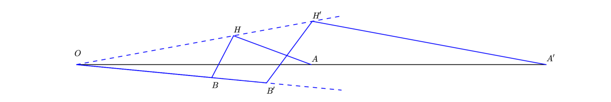
Figure 12: Illustration of double-lens degeneracy. As in Fig. 4, all observables are identical for both the prime and un-primed geometries, including all pairwise delays and angular positions. This degeneracy also holds in three dimensions.

In this archival data set, the direct single lens from the further plane at position $J$ is missing. It would have been visible $59$ days earlier. The difference in time delays to image $J$ and the double reflection images would allow a direct determination of the effective distance to lens plane 2. Due to the close to $90\degree$ angle $\angle~{}DAJ$ between lenses, the effect would be about a factor of 10 ill conditioned. With sufficiently precise VLBI imaging one could distinguish if the doubly-refracted images are at position $B$ (if lens 1 is closer to the observer) or position $H$ (if lens 2 is closer to the observer). As described above, we interpret the effective distances to place screen 2 further away.

3 VLBI astrometry

The model kinematics can be compared to direct measurements of pulsar proper motion to infer the absolute motion of the lensing screen.

PSR B0834+06 was observed 8 times with the Very Long Baseline Array (VLBA), under the project code BB269, between 2009 May and 2011 January. Four 16 MHz bands spread across the frequency range 1406 – 1692 MHz were sampled with 2 bit quantization in both circular polarizations, giving a total data rate of 512 Mbps per antenna. The primary phase calibrator was J0831+0429, which is separated from the target by 2.1 degrees, but the target field also included an in-beam calibrator source J083646.4+061108, which is separated from PSR B0834+06 by only 5 ′. The cycle time between primary phase calibrator and target field was 5 minutes, and the total duration of each observation was 4 hours.

Standard astrometric data reduction techniques were applied (e.g., Deller et al., 2012; Deller et al., 2013), using a phase calibration solution interval of 4 minutes for the in-beam calibrator source J083646.4+061108. J083646.4+061108 is weak (flux density $\sim$4 mJy) and its brightness varied on the level of tens of percent. The faintness leads to noisy solutions, and the variability indicates that source structure evolution (which would translate to offsets in the fitted target position) could be present. Together, these two effects lead to reduced astrometric precision compared to that usually obtained with VLBI astrometry using in-beam calibration, and the results presented here could be improved upon if the observations were repeated using the wider bandwidths and higher sensitivity now available with the VLBA, potentially in conjunction with additional in-beam background sources.

While a straightforward fit to the astrometric observables yields a pulsar distance with a formal error $<$1 per cent, the reduced $\chi^{2}$ of this fit is $\sim$40, indicating that the formal position errors greatly underestimate the true position errors, and that systematic effects such as the calibrator effects discussed above as well as residual ionospheric errors dominate. Accordingly, the astrometric parameters and their errors were instead obtained by bootstrap sampling (Efron & Tibshirani, 1991). These results are presented in Table 5.

Table 5: Fitted and derived astrometric parameters for PSR B0834+06.

Reference right ascension (J2000)a	08:37:5.644606(9)
Reference declination (J2000)a	06:10:15.4047(1)
Position epoch (MJD)	55200
$\mu_{\mathrm{R.A.}}$ (mas yr-1)	2.16(19)
$\mu_{\mathrm{Dec}}$ (mas yr-1)	51.64(13)
Parallax (mas)	1.63(15)
Distance (pc)	620(60)
$v_{\mathrm{T}}$ (km s-1)	150(15)

• The errors quoted here are from the astrometric fit only and do not include the $\sim$1 mas position uncertainty transferred from the in–beam calibrator’s absolute position.

4 Discussions

4.1 Interpretation

The relative motion between pulsar and lens is directly measured by the differential frequency, and not sensitive to details of this model. B10 derived similar motions. This motion is in broad agreement with direct VLBI proper motion measurement, requiring the lens to be moving slowly compared to the pulsar proper motion or the LSR. The lens is $\sim 200$ pc above the Galactic disk. Matter can either be in pressure equilibrium, or in free-fall, or some combination thereof. In free fall, one expects substantial motions. These data rule out retrograde or radially Galactic orbits: the lens is co-rotating with the Galaxy. In pressure equilibrium, gas rotates slower as its pressure scale height increases, which appears consistent with the observed slightly slower than co-rotating motion. The modest lens velocities also appear consistent with the general motion of the ISM, perhaps driven by Galactic fountains (Shapiro & Field, 1976) at these latitudes above the disk. In the inclined sheet model, the waves move at Alfvénic speed, but due to the high inclination, will move less than one percent of this speed in projection on the sky, and thus be completely negligible compared to other sources of motion.

Alternative models, for example, evaporating clouds (Walker & Wardle, 1998) or strange matter (Pérez-García et al., 2013), do not make clear predictions. One would expect higher proper motions from these freely orbiting sources, and larger future scintillation samples may constrain these models.

In order to incline one sheet randomly to better than 1 per cent requires of order $10^{4}$ randomly placed sheets, i.e. many per parsec. This sheet extends for $\sim$ 10 AU in projection, corresponding to a physical scale greater than $1000$ AU. These two numbers roughly agree, leading to a physical picture of magnetic domain boundaries every $\sim 0.1$ pc. B0834+06 has had noted arcs for multiple years, perhaps suggesting this dominant lens plane is larger than typical. One might expect to reach the end of the sheet within decades.

A generic prediction of the inclined sheets model is a change in rotation measure across the scattering length. Over 1000 AU, one might expect a typical RM (rotation measure) change of $10^{-3}$ rad/m². At low frequencies, for example in LOFAR or GMRT, the size of the scattering screen extends another order of magnitude in angular size, and the RM in different lensed images are different, increasing to $\sim 0.01$, which is plausibly measurable. Even for an un-polarized source, the left and right circularly polarized (LCP, RCP) dynamic spectra will be slightly different. Usually a secondary spectrum (SS) is formed by Fourier transforming the dynamic spectrum and multiplying by its complex conjugate. To measure the RM, one multiplies the Fourier transform of the LCP dynamic spectrum by the complex conjugate of the RCP Fourier transform. This will display a phase gradient along the Doppler frequency axis. In the SS, each pixel is the sum of correlations of pairs of scattering points with corresponding lag and Doppler velocity. The velocity is typically linear in the pair separation, which is also the case for differential RM. This statistic is analogous to the cross gate secondary spectrum as applied in Pen et al. (2014).

4.2 Possible improvements

We discuss several strategies which can improve on the solution accuracy. The single biggest improvement would be to monitor the speckle pattern over several months, as the pulsar crosses each individual lens, including both lensing systems. This allows a direct comparison of single lens to double-lens arclets.

Angular resolution can be improved using longer baselines, for example adding a GMRT-GBT baseline doubles the resolution. Observing at multiple frequencies over a longer period allows for a more precise measurement: when the pulsar is between two lenses, the refraction angle $\beta$ is small, and one expects to see the lensing at higher frequency, where the resolution is higher, and distances between lens positions can be measured to much higher accuracy.

Holographic techniques (Walker et al., 2008; Pen et al., 2014) may be able to measure delays, fringe rates, and VLBI positions substantially more accurately. Combining these techniques, the interstellar lensing could conceivably achieve distance measurements an order of magnitude better than the current published effective distance errors. This could bring most pulsar timing array targets into the coherent timing regime, enabling arc minute localization of gravitational wave sources, lifting any potential source confusion.

Ultimately, the precision of the lensing results would be limited by the fidelity of the lensing model. In the inclined sheet model, the images move along fold caustics. The straightness of these caustics depends on the inclination angle, which in turn depends on the amplitude of the surface waves. This analysis concludes a high degree of inclination, and thus high fidelity for geometric pulsar studies.

5 Conclusions

We have applied the inclined sheet model (Pen & Levin, 2014) to archival apex data of PSR B0834+06. The data is well-fit by two linear lensing screens, with nearly plane-parallel geometry. The second screen provides a precision test with 10 observables (5 time delays and 5 differential frequencies) and 3 free parameters (the marked points in Table 3). The model fits the data to $\sim$ percent accuracy on each of 7 data points. This natural consequence of very smooth reconnection sheets is an unlikely outcome of ISM turbulence. These results, if extrapolated to multi-epoch observations of binary systems, might result in accurate distance determinations and opportunities for removing scattering induced timing errors. This approach also opens the window to measuring precise transverse motions of the ionized ISM outside the Galactic plane.

6 Acknowledgements

We thank NSERC for support. We acknowledge helpful discussions with Peter Goldreich and M. van Kerkwijk. We thank Michael Williams for photography help. Siqi Liu thanks Robert Main and JD Emberson for helpful discussions on improving the expression of the content. The National Radio Astronomy Observatory is a facility of the National Science Foundation operated under cooperative agreement by Associated Universities, Inc.

References

- Arnold (1990) Arnold V. I., 1990, Singularities of Caustics and Wave Fronts. Springer Netherlands
- Boyle & Pen (2012) Boyle L., Pen U.-L., 2012, Phys. Rev. D, 86, 124028
- Braithwaite (2015) Braithwaite J., 2015, MNRAS, 450, 3201
- Brisken et al. (2010) Brisken W. F., Macquart J.-P., Gao J. J., Rickett B. J., Coles W. A., Deller A. T., Tingay S. J., West C. J., 2010, ApJ, 708, 232
- Clegg et al. (1998) Clegg A. W., Fey A. L., Lazio T. J. W., 1998, ApJ, 496, 253
- Deller et al. (2012) Deller A. T., Archibald A. M., Brisken W. F., Chatterjee S., Janssen G. H., Kaspi V. M., Lorimer D., Lyne A. G., McLaughlin M. A., Ransom S., Stairs I. H., Stappers B., 2012, ApJ, 756, L25
- Deller et al. (2013) Deller A. T., Boyles J., Lorimer D. R., Kaspi V. M., McLaughlin M. A., Ransom S., Stairs I. H., Stovall K., 2013, ApJ, 770, 145
- Efron & Tibshirani (1991) Efron B., Tibshirani R., 1991, Science, 253, 390
- Goldreich & Sridhar (2006) Goldreich P., Sridhar S., 2006, ApJ, 640, L159
- Kramer et al. (2006) Kramer M., Stairs I. H., Manchester R. N., McLaughlin M. A., Lyne A. G., Ferdman R. D., Burgay M., Lorimer D. R., Possenti A., D’Amico N., Sarkissian J. M., Hobbs G. B., Reynolds J. E., Freire P. C. C., Camilo F., 2006, Science, 314, 97
- Longuet-Higgins (1960) Longuet-Higgins M. S., 1960, J. Opt. Soc. Am., 50, 845
- Lorimer & Kramer (2012) Lorimer D. R., Kramer M., 2012, Handbook of Pulsar Astronomy. Cambridge University Press
- Pen & King (2012) Pen U.-L., King L., 2012, MNRAS, 421, L132
- Pen & Levin (2014) Pen U.-L., Levin Y., 2014, MNRAS, 442, 3338
- Pen et al. (2014) Pen U.-L., Macquart J.-P., Deller A. T., Brisken W., 2014, MNRAS, 440, L36
- Pérez-García et al. (2013) Pérez-García M. Á., Silk J., Pen U.-L., 2013, Physics Letters B, 727, 357
- Shapiro & Field (1976) Shapiro P. R., Field G. B., 1976, ApJ, 205, 762
- Stinebring et al. (2001) Stinebring D. R., McLaughlin M. A., Cordes J. M., Becker K. M., Goodman J. E. E., Kramer M. A., Sheckard J. L., Smith C. T., 2001, ApJ, 549, L97
- Walker & Wardle (1998) Walker M., Wardle M., 1998, ApJ, 498, L125
- Walker et al. (2008) Walker M. A., Koopmans L. V. E., Stinebring D. R., van Straten W., 2008, MNRAS, 388, 1214