Lissajous and Fourier knots

Abstract

We prove that any knot of $\mathbb{R}^{3}$ is isotopic to a Fourier knot of type $(1,1,2)$ obtained by deformation of a Lissajous knot.

1 Introduction

Fourier knots are closed embedded curves whose coordinate functions are finite Fourier sums. Lissajous knots (defined in [BHJS]) are the simplest examples : each coordinate function consists in only one term. Lissajous knots are Fourier knots of type (1,1,1) (cf. for example [K], [La2],[T]).
Surprisingly - at least at first sight - not every isotopy class of knots can be represented by Lissajous knots. Indeed Lissajous knots are isotopic to their mirror image; in particular a nontrivial torus knot cannot be isotopic to a Lissajous knot.

Let us first recall how to construct knots from a knot shadow.

A knot shadow is a generic projection of a knot on a plane. It is a closed planar curve with nodes, i.e. double points. Conversely given a shadow - i.e. an oriented planar closed curve with double points :

$$D:t\mapsto\gamma(t)=\left(x\left(t\right),y\left(t\right)\right)\in\mathbb{R}^{2},$$

we can construct a knot in $\mathbb{R}^{3}$ by defining a height function ${\bf z}$ which has the right values at each node of the shadow. The knot is then defined by:

$${\bf K}:t\mapsto\left(x\left(t\right),y\left(t\right),{\bf z\left(t\right)}\right)\in\mathbb{R}^{3}.$$

Thus a Lissajous knot projects onto a Lissajous shadow ($x(t)$ and $y(t)$ are cosine functions). Although we cannot represent any knot by a Lissajous knot, still any knot $K$ is isotopic to a knot which projects onto a Lissajous shadow ([La]). In other words one can choose $D$ to be a Lissajous shadow but one cannot always choose $z(t)=\cos(pt+\phi)$ as the height function. However, this is possible if the height function $z$ is a Fourier sum of a non prescribed finite number of terms (cf. for instance [K]).
It was conjectured in [La2] that any knot can be presented by a Lissajous diagram with a height function consisting of a Fourier sum with a fixed number of terms or even, as it was suggested experimentally in [BDHZ], with a height function consisting of only two terms: namely

Theorem 1.

Any knot in $\mathbb{R}^{3}$ is isotopic to a Fourier knot of type (1,1,2).

The technique of the proof of theorem 1 is inspired by a paper of [KP] and uses Kronecker’s theorem. Another key property of number theory that will also be used is related to the fact that the only rational values of $\sin\frac{2\pi p}{q}$- for integers $p$ and $q$- are only $0,\pm 1,\pm 1/2$.
The main idea goes as follows: given a knot $K$ in a given isotopy class of knots, we show that it can be presented by a Lissajous diagram with prime frequencies. We then deform the shadow so that nodes are in “general position”, i.e. their parameters are rationally linearly independent. This will be derived from the fact that the nodal curve of the deformation is skewed in the parameter space of all nodes. We then find an integer $n$ and real number $\phi$ -small- such that the height function $h(t):=\cos\left[2n\pi\left(t+\phi\right)\right]$ has the right intersection signs for every two values of the parameter $t$ corresponding to a node of the Lissajous shadow. The height function then defines a third coordinate function which together with the deformed Lissajous shadow coordinates defines a curve of $\mathbb{R}^{3}$ in the given isotopy class.

The paper is organized as follows : In Section 2 and 3 we fix notations and terminology. We compute the node parameters of deformations of Lissajous planar curves in section 4; we also show that any knot admits a Lissajous diagram with prime frequencies.
In Section 5, we show that the nodal curves of our deformations are skewed : for an appropriate choice of deformation parameters and a simple choice of phases, we can compute the determinant of the $k$-th derivatives $k=1,\cdots,n_{D}$ of the nodal curve position vector in $\mathbb{R}^{n_{D}}$ and show that it is not zero. In Section 5.7, the determinant is expressed as a product of factors, each of which is proved to be different from zero. We also show that the skewness of the nodal curve implies that nodes parameters of the diagram are rationally linear independent for a dense subset of the deformation parameter. The last section is devoted to the proof of the theorem : Kronecker’s theorem applied to $\mathbb{Q}$-linear independence of nodal coordinates allows us to choose, as height function of any knot represented by an appropriate Lissajous shadow, a cosine function with appropriate frequency.
Acknowledgement : the starting point of this paper was a fruitful meeting with P-V Koseleff whom we thank heartfully.

Contents

1. 1 Introduction
2. 2 Terminology
   1. 2.1 Knots in $\mathbb{R}^{3}$
   2. 2.2 Deformation of a knot shadow and nodal curve
3. 3 Fourier Knots
   1. 3.1 Lissajous knots
   2. 3.2 Torus knots
4. 4 Nodes and deformations of knot shadows
   1. 4.1 Lissajous Figures, nodes and symmetries
   2. 4.2 Nodes parameters of Lissajous planar curves
   3. 4.3 Prime knot diagrams
   4. 4.4 Nodes coupling
   5. 4.5 Deformations of planar Lissajous curves
   6. 4.6 The nodal curve of a deformation of Lissajous curves
5. 5 $\mathbb{Q}$-Linear dependence of the nodal curve coordinates
   1. 5.1 Infinitesimal deformation and $\mathbb{Q}$-linear independence
   2. 5.2 The Lissajous nodal curve is skewed
   3. 5.3 General form of the nodal curve coordinates
   4. 5.4 Series expansion of nodal curves
   5. 5.5 Series expansion of the nodal curve’s Wronskian
   6. 5.6 The Wronskian is not zero
   7. 5.7 The lowest order term $D_{0}$ of the Wronskian is not zero
   8. 5.8 $\mathbb{Q}$-linear dependence of nodal curves coordinates
6. 6 Proof of the Theorem
   1. 6.1 Kronecker’s theorem

2 Terminology

2.1 Knots in $\mathbb{R}^{3}$

We will consider knots in $\mathbb{R}^{3}$ as presented by a smooth embedding of the circle:

$$\left(\begin{array}[]{cc}\gamma:\mathbb{S}^{1}=\mathbb{R}/\mathbb{Z}&\longrightarrow\mathbb{R}^{3}=\mathbb{R}^{2}\times\mathbb{R}\\ t&\mapsto\left(\gamma_{D}(t),z\left(t\right)\right)\end{array}\right)$$ (1)

where the height function $z$ is a smooth function $\mathbb{S}^{1}\longrightarrow\mathbb{R}$. The planar curve $\gamma_{D}$ is a knot shadow, if it is furthermore a smooth immersion such that the self-intersections of $\gamma_{D}$ are transverse double points also called nodes. Hence for any node $P\in\gamma_{D}(\mathbb{S}^{1})$ there exists a pair of distinct real numbers $s,t\in[0,1[$ such that $\gamma_{D}(s)=\gamma_{D}(t)=P$. We choose for each node one of these two parameters and denote it by $t_{P}\in[0,1[$. It will be convenient to denote the set of nodes by an ordered set $J$ of points and define accordingly the nodal vector $\eta_{0}$ of $\gamma_{D}$ by the $n_{D}$-uplet $(t_{P})_{P\in J}$ $[0,1[^{n_{D}}$, where $n_{D}$ is the number of nodes of curve $\gamma_{D}$.
Conversely given a knot shadow $\gamma_{D}$, and a height function $z(t)$, we can define a knot as in expression (1) if, for each node $P$ of the shadow and for each corresponding pair of parameters $\{s,t\}$ of $P$ , $z(s)-z(t)\not=0$. In fact the knot thus obtained is entirely defined by curve $\gamma_{D}$ and the data $sign(z(s)-z(t))$ for each node. In other words a knot is defined by a shadow $D$ and a height function $z$, where each node of $D$ is parametrized by a pair of real numbers $\{s,t\}$ such that $\gamma_{D}(s)=\gamma_{D}(t)$ and the sign of $z(t)-z(s)$ defines which strand of $\gamma$ lies above which one at a crossing point-or node- of $\gamma_{D}$.

2.2 Deformation of a knot shadow and nodal curve

A deformation of a shadow $\gamma_{D}$ is a smooth family of curve shadows $\{\gamma_{D,\epsilon}\}_{\epsilon\in I}$ where $\epsilon$ lies in the interval of deformation $I=[0,\epsilon_{0}]$ and such that $\gamma_{D,0}=\gamma_{D}$. We associate to a shadow deformation the nodal curve $\eta:[0,\epsilon_{0}]\longrightarrow[0,1]^{n_{D}}$ defined as follows. For each node $P_{i}$, $i=1,\cdots,n_{D}$, of the deformed shadow and ordered in a certain way, there is a pair of two parameters $\{s_{i}(\epsilon),t_{i}(\epsilon)\}$ such that $\gamma_{D}(s_{i})=\gamma_{D}(t_{i})=P_{i}$. We choose one of the two parameters, say $t_{i}$ and the nodal curve is then defined by $\eta(\epsilon)=\left(t_{j}\left(\epsilon\right)\right)_{j=1,\cdots,n_{D}}.$

3 Fourier Knots

We give a quick reminder of some geometric knot presentations that are of some interest in our topic: Fourier knots, Lissajous knots and torus knots that all belong to next family.
A Fourier knot -of type $(m,n,p)$- is a parametrized curve of $\mathbb{R}^{3}$ defined by :

$$F_{m,n,p}:\left(\begin{array}[]{cc}[0,1[&\longrightarrow\mathbb{R}^{3}\\ t&\mapsto F_{m,n,p}(t)\end{array}\right)$$ (2)

with

$$F_{m,n,p}(t)=\left(\sum_{i=1}^{m}M_{i}\cos(2\pi m_{i}t+\phi_{i}),\sum_{i=1}^{n}N_{i}\cos(2\pi n_{i}t+\psi_{i}),\sum_{i=1}^{p}P_{i}\cos(2\pi p_{i}t+\tau_{i})\right)$$

for some $\phi_{i},M_{i},N_{i},\psi_{i},,\tau_{i},P_{i}\in\mathbb{R}$ and $m_{i},n_{i},p_{i}\in\mathbb{N}$.
It was proved in [La2] that any knot $K$ is isotopic to a curve of type $(1,1,n_{K})$ where $n_{K}$ depends on the knot.

3.1 Lissajous knots

Fourier knots of type $(1,1,1)$ are also called Lissajous knots and have been extensively studied in [BHJS]).

$$L(n_{1},n_{2},n_{3},\phi_{1},\phi_{2}):\left(\begin{array}[]{ll}[0,1]&\longrightarrow\mathbb{R}^{3}\\ t&\mapsto\left(\cos 2\pi n_{1}t,\cos 2\pi n_{2}\left(t+\phi_{1}\right),\cos 2\pi n_{3}\left(t+\phi_{2}\right)\right)\end{array}\right)$$ (3)

,

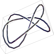
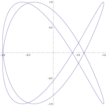
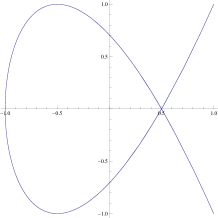
Figure 1: knot $L(2,3,5,0,.2,2)=6_{1}$, shadow $L(2,3,.2)$, and associated Chebyshev figure $C(2,3)$

It is noteworthy to recall that Lissajous knots are topologically equivalent to closed billiard trajectories in a cube. (cf. [JP]) These Lissajous knots project horizontally on planar Lissajous curves of type $L(n_{1},n_{2},\phi_{1})$.
When the phase $\phi_{1}$ is zero, the Lissajous figure degenerates into a 2-1 curve $C(n_{1},n_{2})$ which is a subset of an algebraic Chebyshev open curve as defined in [KP]:

$$T(n_{1},n_{2})=\{(x,y):T_{n_{1}}(x)=T_{n_{2}}(y)=0\},$$

where $T_{n}$ is the Chebyshev polynomial of degree $n$ (see fig. 1).
Although not all knot are Lissajous knots, [KP] showed that, for suitable numbers $n_{1},n_{2},n_{3}$ and phase $\phi$, any knot is isotopic a Chebyshev knot obtained by Alexandrov compactification of a curve $T(n_{1},n_{2},n_{3},\phi):\mathbb{S}^{1}\longrightarrow\mathbb{R}^{3}$ with $T(n_{1},n_{2},n_{3},\phi)(t)=(T_{n_{1}}(t),T_{n_{2}}(t),T_{n_{3}}(t+\phi)).$

3.2 Torus knots

Another key family of Fourier knots are torus knots -neither of which can be isotopic to a Lissajous knot (except the trivial ones)! A Torus knot $T(p,q)$ is originally defined as an embedding of $\mathbb{S}^{1}$ onto a torus as a Fourier knot of type $(3,3,1)$ :

$$T(p,q)(t)=\left(\cos 2\pi qt\left(1+\frac{1}{2}\cos 2\pi pt\right),\sin 2\pi qt\left(1+\frac{1}{2}\cos 2\pi pt\right),\sin 2\pi pt\right).$$

But it was shown in [H] that torus knots $T(p,q)$’s are isotopic to Fourier knots of type $(1,1,2)$ :

$$T(p,q)(t)=\left(\cos 2\pi pt,\cos 2\pi q\left(t+\frac{1}{4p}\right),\cos 2\pi\left(pt+\frac{1}{4}\right)+\cos 2\pi\left(\left(q-p\right)t+\frac{1}{4p}\right)\right)$$

4 Nodes and deformations of knot shadows

We first recall some basic properties of Lissajous planar curves and compute the positions of its nodes.
In the second part of the section we add a small perturbation term to one of the two coordinates; we define a family of perturbed Lissajous planar curves which are very close to the original Lissajous figure. We then describe the positions of the nodes as functions of the deformation parameter $\epsilon$.

4.1 Lissajous Figures, nodes and symmetries

We need to give some precisions on the Lissajous curves :

$$L(n_{1},n_{2},\phi):\left(\begin{array}[]{ll}[0,1]&\longrightarrow\mathbb{R}^{2}\\ t&\mapsto\left(\cos\left(2\pi n_{1}t\right),\cos\left(2\pi n_{2}t+\phi\right)\right)\end{array}\right)$$ (4)

We will suppose that $n_{1}$ and $n_{2}$ are coprime (otherwise $L$ is not 1-1). We can also suppose for our purpose that the phase $\phi$ is a small positive irrational number. Our first goal is to find the expression of the ordered pairs of parameters $(t_{i},s_{i}),i=1,\cdots N$ corresponding to the double points $P_{i},i=1,\cdots,N$ of a Lissajous figure.

,

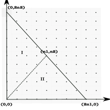
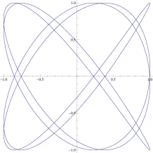
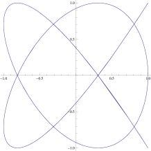
Figure 2: 31 Nodes parametrized by integer points in triangle $\Delta$ of Lissajous $L(4,5,.1)$, and associated Chebyshev $C(4,5)$

,

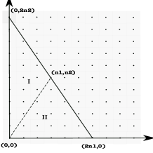
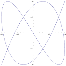
Figure 3: 22 nodes parametrized by integer points of Lissajous curve $L(3,5,.1)$ with 10 nodes of type I, and associated Chebyshev $C(3,5)$

In the degenerate case where the phase $\phi$ is zero we obtain a $2-1$ curve (see figure 2 and 3). This curve is a subset of a Chebyshev curve defined in [KP] and which is an open algebraic curve.

4.2 Nodes parameters of Lissajous planar curves

We need to compute the node parameters of a planar Lissajous curve. Such a parametrization was already published (cf. for instance [BDHZ] or [JP]). But we derive it again to get a geometric representation of these nodes as a set of integer points that lie in a straight rectangle: we will use symmetries of this set for our computations.
We may notice first that the number of nodes of a Lissajous figure is easily deduced from the number of nodes $n_{C(n_{1},n_{2})}:=\frac{(n_{1}-1)(n_{2}-1)}{2}$ of its associated Chebyshev curve (cf. for example [Pe]). As the phase $\phi$ becomes positive, each node of the Chebyshev curve blows up into four nodes. Moreover each pair of maxima or minima of the coordinates functions $x(t),y(t)$ give also rise to a node (except for $t=0,\pm 1,\pm 1/2$) ; this produces $n_{L(n_{1},n_{2},\phi)}=4\frac{(n_{1}-1)(n_{2}-1)}{2}+n_{1}+n_{2}-2=2n_{1}n_{2}-n_{1}-n_{2}$.
More precisely, given a node $P$, let us find the double parameters $(t_{P},s_{P})$ such that $L(t_{P})=L(s_{P})=P$.
Equality for the first coordinate yields :

$$\cos 2\pi n_{1}t=\cos 2\pi n_{1}s$$

iff

$$s=\sigma t+\frac{k}{n_{1}},\quad\sigma=\pm 1\quad k\in\mathbb{Z}$$ (5)

Equality for the second coordinate yields :

$$\cos\left[2\pi n_{2}\left(t+\phi\right)\right]=\cos\left[2\pi n_{2}\left(s+\phi\right)\right]$$ (6)

Plug equality (5) into (6) :

$$\cos 2\pi n_{2}\left(t+\phi\right)=\cos 2\pi n_{2}\left(\sigma t+\frac{k}{n_{1}}+\phi\right)$$ (7)

and apply again (5) :

$$\sigma t+\frac{k}{n_{1}}+\phi=\sigma^{\prime}\left(t+\phi\right)+\frac{l}{n_{2}}\quad\sigma^{\prime}=\pm 1\quad k\in\mathbb{Z}$$ (8)

We get two sets of solutions according to the choice of $\sigma$ and $\sigma^{\prime}$ :

1. Type I. If $\sigma=1$ and $\sigma^{\prime}=-1$ then :

   $$t=-\phi+\frac{1}{2}\left(\frac{l}{n_{2}}-\frac{k}{n_{1}}\right)$$ (9)

   Hence

   $$s=t+\frac{k}{n_{1}}=-\phi+\frac{1}{2}\left(\frac{l}{n_{2}}+\frac{k}{n_{1}}\right)$$ (10)

   Since $s,t\in[0,1[$, the integer points $(k,l)$ necessarily lie in a parallelogram $\mathcal{P}$ which is defined by conditions :

   $$\left\{\begin{array}[]{ccc}2\phi n_{1}n_{2}\leq&n_{1}l-n_{2}k<&(1+\phi)2n_{1}n_{2}\\ 2\phi n_{1}n_{2}\leq&n_{1}l+n_{2}k<&(1+\phi)2n_{1}n_{2}\end{array}\right.$$ (11)

   As phase $\phi$ is small, parallelogram $\mathcal{P}$ is obtained by a small translation of the parallelogram with vertices $(0,0),(n_{1},n_{2}),(-n_{1},n_{2}),(0,2n_{2})$. Since $n_{1}$ and $n_{2}$ are coprime there are only the 4 integer points vertices on the boundary of the translated parallelogram.
   

2. Type II. In the second case, $\sigma=-1$, $\sigma^{\prime}=1$ and we obtain :

   $$t=\frac{1}{2}\left(\frac{k}{n_{1}}-\frac{l}{n_{2}}\right)$$ (12)

   Hence

   $$s=\frac{1}{2}\left(\frac{l}{n_{2}}+\frac{k}{n_{1}}\right)$$ (13)

   And conditions $s,t\in[0,1[$ yields - we recall that $\phi$ is very small-

   $$\left\{\begin{array}[]{ccc}0\leq&n_{2}k-n_{1}l<&2n_{1}n_{2}\\ 0\leq&n_{2}k+n_{1}l<&2n_{1}n_{2}\end{array}\right.$$ (14)

   Solutions are given by integer points $(k,l)\in\mathcal{P}^{\prime}$ which is a small translation of the parallelogram with vertices $(0,0),(n_{1},n_{2}),(n_{1},-n_{2}),(2n_{1},0)$.

For each solution found, one should check that $s\not=t$ and also that pairs $\{t,s\}$ corresponding to the same node are not counted twice.
For each pair of solutions $\{s,t\}$, condition $s\not=t$ implies $k\not=0$ for the first type and $l\not=0$ in the second case; furthermore for points of type I the transformation : $k\mapsto-k$ permutes $t$ and $s$ which are parameters that correspond to the same node. Hence we can reduce the parameter set of nodes to the isosceles triangle $\Delta^{I}:=\{(k,l)\in\mathcal{P}:k>0\}$ and similarly for type II points : $\Delta^{II}:=\{(k,l)\in\mathcal{P}^{\prime}:l>0\}$. In The union of $\Delta^{I}$ and $\Delta^{II}$ defines a straight triangle $\Delta$ (see figure 5 a)). In summary :

Lemma 1.

A generic Lissajoux planar curve $L(n_{1},n_{2},\phi)$, with $n_{1}$ and $n_{2}$ coprime and $\phi$ small, and defined by

$$L(n_{1},n_{2},\phi):\left(\begin{array}[]{c}[0,1]\longrightarrow\mathbb{R}^{2}\\ t\mapsto\left(\cos 2\pi n_{1}t,\cos\left[2\pi n_{2}\left(t+\phi\right)\right]\right)\end{array}\right)$$ (15)

has $n_{L(n_{1},n_{2},\phi)}=2n_{1}n_{2}-n_{1}-n_{2}$ nodes parametrized by the integer points that lie in the interior of the straight triangle $\Delta$ :
$J=\Delta\cap\mathbb{N}\times\mathbb{N}:=\{(k,l):k>0,l>0,n_{2}k+n_{1}l<2n_{1}n_{2}\}$.
The node vector is by definition $(t_{j})_{j\in J}\in[0,1[^{n_{L(n_{1},n_{2},\phi)}}$ where,
for each $(k,l)\in J$:

$$t_{kl}:=\left\{\begin{array}[]{cc}-\phi+\frac{1}{2}\left(-\frac{k}{n_{1}}+\frac{l}{n_{2}}\right)&\quad{\rm if}\quad n_{1}l>n_{2}k\quad{\rm(type\ I)}\\ \frac{1}{2}\left(\frac{k}{n_{1}}-\frac{l}{n_{2}}\right)&\quad{\rm if}\quad n_{1}l<n_{2}k\quad{\rm(type\ II)}\end{array}\right.$$ (16)

4.3 Prime knot diagrams

           

Figure 4: $C(4,5)$, billiard curve $L(4,5,.1)$ and plat-closure braid of $L(4,5,.1)$

We first recall that a checkerboard - such as $L(n_{1},n_{2})$- is the plat-closure (cf. [B]) of a braid of $2n_{1}$ strands defined by the following group element of the braid group $B_{2n_{1}}$:

$$C(2n_{1},n_{2}-1):=\left(\sigma^{*}_{2}\sigma^{*}_{4}\cdots\sigma^{*}_{2n_{1}-2}\sigma^{*}_{1}\sigma^{*}_{3}\cdots\sigma^{*}_{2n_{1}-1}\right)^{n_{2}-1}\sigma^{*}_{2}\sigma^{*}_{4}\cdots\sigma^{*}_{2n_{1}-2}$$

(the powers of $\sigma_{i}$, denoted by$*$ are $\pm 1$; they are irrelevant as far as the shadow is concerned).

C. Lamm showed in his thesis (cf [La2] Theorem 2.3) that any knot is presented by a checkerboard diagram $C_{k}(2n_{1},2n_{1}.p)$ for some $p$. This diagram has a Lissajous shadow of type $L(n_{1},n_{2}=2n_{1}p+1)$. Hence we can as well say that any knot is presented by a Lissajous diagram.

Proposition 1.

Any knot admits a Lissajous diagram with shadow $L(n_{1},n_{2})$ where $n_{1}$ and $n_{2}$ are odd primes and where $n_{2}\equiv 1\ {\textrm{m}od\ }n_{1}$.

Proof : the only constraint on $n_{1}$ is that it should be greater or equal to the braid index of $K$. In particular choosing $n_{1}$ large enough, we can suppose that $n_{1}$ is prime and odd. Moreover from the proof of theorem 2.3 of [La2], we can also represent the same knot by diagrams with shadows $L(n_{1},n_{2}=2n_{1}(p+q)+1)$ for any nonnegative number $q$: $q$ represents the number of pure braids added to the original rosette braid. For each added piece and by a judicious choice of the crossing numbers the new rosette braid represents the same knot. By Dirichlet’s prime number theorem and since $2n_{1}$ and $n_{2}$ are rel. prime, there are numbers $q$ such that $n_{2}$ is prime. We will thus restrict our further investigation of the Lissajous figure to the case where $n_{1}$ and $n_{2}$ are odd primes.

4.4 Nodes coupling

                 

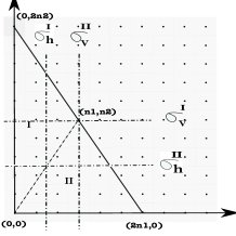
Figure 5: Triangle $\Delta=\Delta^{I}\cup\Delta^{II}$; hor. and vert. symmetries

We describe a method to pair the nodes which will be crucial in section 5.

We will regroup integer points of the triangle $\Delta$, described in Lemma 1, by pairs. The $n_{1}n_{2}-n_{2}$ nodes of type I (resp. the $n_{1}n_{2}-n_{1}$ nodes of type II) are parametrized by the integer points of the isoceles subtriangle $\Delta^{I}:=\left(\left(0,0\right),\left(n_{1},n_{2}\right),\left(0,2n_{2}\right)\right)\subset\Delta$
-resp. $\Delta^{II}:=\left(\left(0,0\right),\left(2n_{1},0\right),\left(n_{1},n_{2}\right)\right)\subset\Delta$- (see fig 5) .

                 

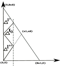
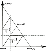
Figure 6: Subdomains of triangle $\Delta$

Lemma 2.

Each node of $\Delta^{I}$ (resp. $\Delta^{II}$) is coupled to a different node of $\Delta^{I}$ (resp. $\Delta^{II}$). The set of pairs extracted from $\Delta^{I}$ (resp. $\Delta^{II}$) are parametrized by integer points lying in the parallelograms :
$\Pi^{I}:=\left(\left(0,0\right),\left(\frac{n_{1}}{2},\frac{n_{2}}{2}\right),\left(\frac{n_{1}}{2},n_{2}+\frac{n_{2}}{2}\right),\left(0,n_{2}\right)\right)$
(resp. $\Pi^{II}:=\left(\left(0,0\right),\left(\frac{n_{1}}{2},\frac{n_{2}}{2}\right),\left(n_{1}+\frac{n_{1}}{2},\frac{n_{2}}{2}\right),\left(n_{1},0\right)\right)$)(see figure 5).

Proof :

1. We first regroup separately integer points in each isosceles triangle, namely $\Delta^{I}$ and $\Delta^{II}$, using resp. the horizontal symmetry $\sigma^{I}_{h}:(k,l)\longrightarrow(n_{1}-k,l)$ (resp. symmetry $\sigma^{II}_{h}:(k,l)\longrightarrow(k,n_{2}-l)$).
   We pair each integer point above the axis of symmetry with its reflection image. Notice that, since $n_{1}$ and $n_{2}$ are odd, no integer point lies on the axis of $\sigma^{I}_{h}$ (resp. $\sigma^{II}_{h}$). Hence this process forms pairs of distinct points parametrized by integer points in the isosceles triangle (see fig.6)
   $\Delta^{I_{0}}:=\left(\left(0,n_{2}\right),\left(n_{1}/2,n_{2}/2\right),\left(n_{1}/2,3n_{2}/2\right)\right)$.
   (resp. $\Delta^{II_{0}}:=\left(\left(n_{1},0\right),\left(n_{1}/2,n_{2}/2\right),\left(3n_{1}/2,n_{2}/2\right)\right)$).

2. The remaining points of $\Delta^{I}$ that are not yet coupled, form two isosceles subtriangles $\Delta^{I^{\prime}},\Delta^{I^{\prime\prime}}$ -resp $\Delta^{II^{\prime}},\Delta^{II^{\prime\prime}}$ of $\Delta^{II}$- (see figure 5).
   We then couple each point of $\Delta^{I^{\prime}}$ with a point of $\Delta^{I^{\prime\prime}}$ (resp. each point of $\Delta^{II^{\prime}}$ with a point of $\Delta^{II^{\prime\prime}}$) via a translation $\tau^{I}$ of vector $(0,n_{2})$ (resp. via a translation $\tau^{II}$ of vector$(n_{1},0)$ (see fig. 6).
   

Alltogether the set of pairs of nodes are parametrized by the union of two parallelograms $\Pi^{I}:=\Delta^{I^{\prime}}\cup\Delta^{I_{0}}$ and $\Pi^{II}:=\Delta^{II^{\prime}}\cup\Delta^{II_{0}}$. ∎

4.5 Deformations of planar Lissajous curves

Let us consider a deformation of a Lissajous figure $\{L_{\epsilon}(n_{1},n_{2},n_{3},\phi,\psi)\}_{\epsilon\in[0,\epsilon_{0}[}$

$$L_{\epsilon}(n_{1},n_{2},n_{3},\phi,\psi):\left(\begin{array}[]{ll}[0,1]&\longrightarrow\mathbb{R}^{2}\\ t&\mapsto\left(\cos\left(2\pi n_{1}t\right),\cos\left(2\pi n_{2}\left(t+\phi\right)\right)+\epsilon\cos\left(2\pi n_{3}\left(t+\phi+\psi\right)\right)\right)\end{array}\right)$$

These are Fourier curves of type $(1,2)$. The node positions of the curve are shifted as we can see in figure 6 and the symmetry of the initial Lissajous figure is clearly broken.

           

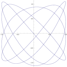
Figure 7: Lissajous shadow $L(4,5,.1)$ and deformation $L_{\epsilon}(4,5,7,.1,.2)$

Let us compute the nodes parameters of these deformed Lissajous planar curves.

4.6 The nodal curve of a deformation of Lissajous curves

Consider a deformation $\{L_{\epsilon}(n_{1},n_{2},n_{3},\phi,\psi)\}_{\epsilon\in[0,\epsilon_{0}]}$ where $n_{1}$ and $n_{2}$ are odd coprimes.
The coordinates of the nodal curve $\eta$ introduced in section 2.2 are ordered according to the lexicographic ordering of integer points of the triangle $\Delta$ described in Lemma 1.We proceed as in this Lemma.

Suppose $L_{\epsilon}(t)=L_{\epsilon}(s)$; then equality of first coordinates yields

$$s=\sigma t+\frac{k}{n_{1}},\quad k\in\mathbb{Z},\quad\sigma=\pm 1.$$ (17)

Equality for the second coordinates yields :

$$\begin{array}[]{l}\cos\left(2\pi n_{2}\left(t+\phi\right)\right)-\cos\left(2\pi n_{2}\left(s+\phi\right)\right)=\\ \epsilon\left(\cos(2\pi n_{3}(s+\phi+\psi))-\cos(2\pi n_{3}(t+\phi+\psi))\right)\end{array}$$ (18)

Or, using formula $\cos a-\cos b=-2\sin(\frac{a+b}{2})\sin(\frac{a-b}{2}),$

$$\begin{array}[]{cc}&\sin\left(2\pi n_{2}\left(\frac{t+s}{2}+\phi\right)\right)\sin\left(2\pi n_{2}\frac{t-s}{2}\right)=\\ &-\epsilon\sin\left(2\pi n_{3}\left(\frac{t+s}{2}+\phi+\psi\right)\right)\sin\left(2\pi n_{3}\frac{t-s}{2}\right).\end{array}$$ (19)

Plug equality (17) into (19); we get two cases according to the value of $\sigma=\pm 1$ :

1. Type I. If $\sigma=+1$ ; $s=t+\frac{k}{n_{1}}$ hence $\frac{s+t}{2}=t+\frac{k}{2n_{1}}$, $k\in\mathbb{Z}$ and $t$ is given implicitely by the equation :

   $$\sin\left(2\pi n_{2}\left(t+\frac{k}{2n_{1}}+\phi\right)\right)a_{k}=\epsilon\sin\left(2\pi n_{3}\left(t+\frac{k}{2n_{1}}+\phi+\psi\right)\right)$$ (20)

   where $a_{k}=-\frac{\sin\left(\pi\frac{n_{2}k}{n_{1}}\right)}{\sin\left(\pi\frac{n_{3}k}{n_{1}}\right)}$ (which is well-defined and not zero since $k<n_{1}$ and $n_{2},n_{3}$ are prime relatively to $n_{1}$).
   Hence for any $\epsilon$, solutions are parametrized by the integer points $(k,l)\in\Delta^{I}$ and given by

   $$t_{kl}(\epsilon):=-\phi+\frac{1}{2}\left(-\frac{k}{n_{1}}+\frac{l}{n_{2}}\right)+u_{kl}(\epsilon)$$ (21)

   where $u_{kl}$ is a function defined implicitely by $f_{kl}\left(u_{kl}\left(\epsilon\right)\right)=\epsilon$ with :

   $$f_{kl}(y)=a_{k}(-1)^{l}\frac{\sin 2\pi n_{2}y}{\sin\left(2\pi n_{3}\left(y+\frac{l}{2n_{2}}+\psi\right)\right)}$$

2. Type II. If $\sigma=-1$ then $s=-t+\frac{k}{n_{1}}$, hence $\frac{t-s}{2}=t-\frac{k}{2n_{1}}$ and

   $$b_{k}\sin\left(2\pi n_{2}\left(t-\frac{k}{2n_{1}}\right)\right)=\epsilon\sin\left(2\pi n_{3}\left(t-\frac{k}{2n_{1}}\right)\right)$$ (22)

   where $b_{k}=-\frac{\sin\left(2\pi n_{2}\left(\frac{k}{2n_{1}}+\phi\right)\right)}{\sin\left(2\pi n_{3}\left(\frac{k}{2n_{1}}+\phi+\psi\right)\right)}$ ($b_{k}$ is not zero and well-defined for small $\phi,\psi$ as for the $a_{k}$’s).

As in case I, solutions are given by

$$t_{kl}(\epsilon):=+\frac{1}{2}\left(\frac{k}{n_{1}}-\frac{l}{n_{2}}\right)+u_{k,l}(\epsilon)$$ (23)

with $f_{kl}\left(u_{kl}\left(\epsilon\right)\right)=\epsilon$ where

$$f_{kl}(y)=b_{k}(-1)^{l}\frac{\sin 2\pi n_{2}y}{\sin\left(2\pi n_{3}\left(y+\frac{l}{2n_{2}}\right)\right)}.$$

Notice that $u_{kl}(0)=0$ and that the $t_{kl}(0)$ are the solutions of type I and II described in Lemma 1. Let us summarize these facts and define the nodal curve of the deformation:

Lemma 3.

Consider a deformation of planar Lissajous curves $L_{\epsilon}(n_{1},n_{2},n_{3},\phi,\psi)$ with $n_{1}$ and $n_{2}$ odd and consider a Lissajous deformation :

$$L_{\epsilon}(n_{1},n_{2},n_{3},\phi,\psi):\left(\begin{array}[]{ll}[0,1]&\longrightarrow\mathbb{R}^{2}\\ t&\mapsto\left(\cos 2\pi n_{1}t,\cos\left[2\pi n_{2}\left(t+\phi\right)\right]+\epsilon\cos\left[2\pi n_{3}\left(t+\phi+\psi\right)\right]\right)\end{array}\right)$$

$\epsilon\in[0,\epsilon_{0}[$, where we suppose that $\epsilon_{0}$ and $\phi$ are small and $n_{1},n_{2},n_{3}$ are relatively prime.
Each planar curve $L_{\epsilon}$ has $n_{L(n_{1},n_{2},\phi)}=2n_{1}n_{2}-n_{1}-n_{2}$ nodes parametrized by the integer points that lie in the interior of the straight triangle $\Delta$ (defined in Lemma 1)
The nodal curve $\eta(\epsilon)=(t_{kl})_{(k,l)\in\Delta}\in[0,1[^{n_{L(n_{1},n_{2},\phi)}}$ is defined by

$$\eta(\epsilon)_{kl}=t_{kl}(\epsilon):=\left\{\begin{array}[]{cc}-\phi+\frac{1}{2}\left(-\frac{k}{n_{1}}+\frac{l}{n_{2}}\right)+u_{kl}(\epsilon)&\quad{\rm if}\ (k,l)\in\Delta^{I}\\ \frac{1}{2}\left(\frac{k}{n_{1}}-\frac{l}{n_{2}}\right)+u_{kl}(\epsilon)&\quad{\rm if}\ (k,l)\in\Delta^{II}.\end{array}\right.$$ (24)

where the $kl$ are lexicographically ordered.
Functions $u_{kl}$ are the local inverse functions of functions $f_{kl}$, ie such that $f_{kl}\circ u_{lk}=Id$.
$\bullet$ If $(k,l)\in\Delta^{I}$ then :

$$f_{kl}(y)=\frac{\sin 2\pi n_{2}y}{a^{I}_{kl}\sin\left[2\pi n_{3}\left(y+\frac{l}{2n_{2}}+\psi\right)\right]},\quad a^{I}_{kl}:=(-1)^{l+1}\frac{\sin\pi\frac{n_{3}k}{n_{1}}}{\sin\pi\frac{n_{2}k}{n_{1}}}$$

$\bullet$ If $(k,l)\in\Delta^{II}$ then :

$$f_{kl}(y)=\frac{\sin 2\pi n_{2}y}{a^{II}_{kl}\sin\left[2\pi n_{3}\left(y+\frac{l}{2n_{2}}\right)\right]},\qquad a^{II}_{kl}:=(-1)^{l+1}\frac{\sin\left[2\pi n_{3}\left(\frac{k}{2n_{1}}+\phi+\psi\right)\right]}{\sin\left[2\pi n_{2}\left(\frac{k}{2n_{1}}+\phi\right)\right]}.$$

5 $\mathbb{Q}$-Linear dependence of the nodal curve coordinates

5.1 Infinitesimal deformation and $\mathbb{Q}$-linear independence

We will give a infinitesimal condition on the curve to ensure the rational linear independence. But first let us prove

Lemma 4.

Let $\gamma:I=[0,\epsilon_{0}]\longrightarrow[0,1]^{n}$ be a real analytic skew curve. Then the set of $\epsilon\in[0,\epsilon_{0}]$ such that the numbers

$$\gamma_{1}(\epsilon),\cdots,\gamma_{n}(\epsilon),1$$ (25)

are rationally linear independent, is dense in $[0,\epsilon_{0}]$.

Proof : we exhibit a sequence of $\epsilon$’s that converges to zero and such that the numbers (25) are rationally linear independent-the same proof will work for any other points $\neq 0$.
If such a sequence does not exist, there is a nonempty neighborhood $I^{\prime}$ of $0$ in $I$ such that the coordinates of $\gamma(\epsilon)$ and $1$ are rationally linear dependent; then

$$\sum_{i=1}^{n}\lambda_{i}(\epsilon)\gamma_{i}(\epsilon)+\lambda_{n+1}(\epsilon)=0.$$

Since $I^{\prime}$ is an uncountable set, the map $\lambda:I^{\prime}\longrightarrow\mathbb{Q}^{n+1}$ takes the same vector value $(\lambda_{i})_{i=1,\cdots,n}$ for infinitely many $\epsilon_{k}$ with $\underset{k\mapsto+\infty}{\lim}\epsilon_{k}=0$. Hence for infinitely many values of $\epsilon_{k}$ converging to $0$ we have

$$\sum_{i=1}^{n}\lambda_{i}\gamma_{i}(\epsilon_{k})+\lambda_{n+1}=0.$$ (26)

Since $\gamma$ is analytic we deduce that this relation is true for all $\epsilon$; hence $\gamma$ belongs to a hyperplane with rational coefficients, which contradicts the skewness of curve $\gamma$. ∎
Similarily we prove

Lemma 5.

If $t_{1},\cdots,t_{n},1$ are rationally lin. independent, then $\{t_{1}+\phi,\cdots,t_{n}+\phi,1\}$ are rationally linear independent for a dense subset of $\mathbb{R}.$

Taking successive derivatives of equation (26) in Lemma 4 we deduce the following infinitesimal criterion for $\mathbb{Q}$-linear independence :

Corollary 1.

Let $\gamma:[0,\epsilon_{0}]\longrightarrow[0,1]^{n}$ be an analytic curve such that a Wronskian is not zero :

$$\left|\begin{array}[]{cccc}\gamma_{1}^{(k_{1})}(0)&\gamma_{1}^{(k_{2})}(0)&\ldots&\gamma_{1}^{(k_{n})}(0)\\ \gamma_{2}^{(k_{1})}(0)&\gamma_{2}^{(k_{2})}(0)&\ldots&\gamma_{2}^{(k_{n})}(0)\\ \vdots&\vdots&\ldots&\vdots\\ \gamma_{n}^{(k_{1})}(0)&\gamma_{n}^{(k_{2})}(0)&\ldots&\gamma_{n}^{(k_{n})}(0)\end{array}\right|\not=0$$ (27)

where $k_{1}<k_{2}<\cdots,k_{n}$; then the set of real numbers $\{1,\gamma_{j}(\epsilon),\ j=1,\cdots,n\}$ are linear independent over $\mathbb{Q}$ for a dense subset of $[0,\epsilon_{0}]$.

5.2 The Lissajous nodal curve is skewed

We will show in this section that

Proposition 2.

Assume that $n_{1},n_{2}$ are odd primes and $n_{3}$ is relatively prime to $n_{1},n_{2}$ and satisfy :

$$\left\{\begin{array}[]{cc}n_{3}&\equiv 2\quad{\textrm{m}od\ }n_{1}\\ n_{3}&\equiv 2\quad{\textrm{m}od\ }n_{2}.\end{array}\right.$$ (28)

Then there are positive real numbers $\epsilon_{0},\phi_{0},\psi_{0}$ such that for any $|\epsilon|\leq\epsilon_{0}$, $|\phi|\leq\phi_{0},|\psi-\frac{\pi}{4}|\leq\psi_{0}$, the nodal curve $\eta(\epsilon)$ of the Lissajous deformation $L_{\epsilon}(n_{1},n_{2},n_{3},\phi,\psi)$ is skewed.

In Subsection 5.3 we give an explicit expression of the nodal coordinates of a Lissajous deformation; we then show, in Subsection 5.5, that the Wronskien $D$ of the nodal curve is a polynomial in $r=\frac{n_{2}}{n_{3}}$; in Subsection 5.7 we compute the coefficient $D_{0}$ of the lowest order monomial.

5.3 General form of the nodal curve coordinates

Consider a curve $Y:$

$$Y:\left(\begin{array}[]{cc}I:=[0,\epsilon_{0}]&\longrightarrow\mathbb{R}^{n}\\ \epsilon&\mapsto\left(y_{j}\right)_{j\in J}\end{array}\right)$$ (29)

with initial position $Y(0)=\left(y_{j}\left(0\right)\right)_{j=1,\cdots,n}$ and let us define curve $U$ such that $Y=Y(0)+U.$ Then :

$$y_{j}(\epsilon)=y_{j}(0)+u_{j}(\epsilon)\ {\rm and}\ u_{j}(0)=0\ \quad\forall\epsilon\in I,j=1,\cdots,n.$$

For each $j=1,\cdots,n$, the $j$-th coordinate function $u_{j}$ of $U$ is defined as the inverse function of a given function $f_{j}$ :

$$f_{j}(u_{j}(\epsilon))=\epsilon\quad\forall\epsilon\in I.$$

Though each coordinate function $u_{j}(\epsilon)$- which we will denote indistinctively by $u(\epsilon)$- is defined implicitely, the Lagrange inversion formula (cf. for instance [S]) yields an explicit power series expansion in terms of $\epsilon$ in the neigborhood of any $0$ :

$$u(\epsilon):=\sum_{n\geq 1}u_{n}(0)\frac{\epsilon^{n}}{n!}$$

Namely :

$$u(\epsilon)=\sum_{n=1}^{\infty}\frac{d^{(n-1)}}{dt^{n-1}}\left(\frac{t}{f(t)}\right)^{n}\biggr{|}_{t=0}\frac{\epsilon^{n}}{n!}.$$ (30)

5.4 Series expansion of nodal curves

Each one of the coordinates of the nodal curve of a Lissajous deformation is defined by the inverse of a real function of the following type :

$$f(u)=\frac{\sin u}{a\sin(ru+\psi)}\qquad(r\in\mathbb{Q},a\in\mathbb{R}^{*},\psi\in\mathbb{R}).$$ (31)

A simple computation using Lagrange’s inverse formula (30) (cf. for example [S]) gives the coefficients $u_{n}(0)$ of the expansion around zero of $u$ such that $f\circ u=Id$:

$$u_{1}(0)=a\sin\psi,u_{2}(0)=a^{2}r\sin\psi\cos\psi,,u_{3}(0)=a^{3}\sin\psi\left(6r^{2}+(1-9r^{2})\sin^{2}\psi\right)\cdots.$$

Lemma 6.

Let $u$ be the inverse function of $f$ defined by equation (31).
For each $n\geq 1$ the n-th coefficient of the power series of $u$ around zero : $\ u_{n}$ equals $a^{n}P_{n}(\sin\psi,\cos\psi,r)$, where $P_{n}$ is a polynomial of degree $n$ w.r.t. variables $\cos\psi$ and $\sin\psi$. $P_{n}$ is also a polynomial in $r$ of degree $n-1$ whose lowest order term is:

$$\bar{u}_{n}(0):=\left\{\begin{array}[]{ll}a^{n}\left(\frac{y}{\sin u}\right)^{n}\biggr{|}_{u=0}^{(n-1)}\sin^{n}\psi&:=a^{n}c_{n}\sin^{n}\psi\quad\hfil(n\ {\rm odd}),\\ r.na^{n}(\frac{y}{\sin u})^{n}\biggr{|}_{u=0}^{(n-2)}\cos\psi\sin^{n-1}\psi&:=a^{n}c_{n}\cos\psi\sin^{n-1}r\psi\quad{\rm(n\ even)}\end{array}\right.$$ (32)

Proof : Lagrange’s inversion formula (30) applied to function (31) and evaluated at zero, yields :

$$u_{n}(0)=a^{n}\left(\left(\frac{y}{\sin y}\right)^{n}\sin^{n}\left(ry+\psi\right)\right)\biggr{|}_{y=0}^{(n-1)}$$

Leibniz formula yields :

$$u_{n}(0)=a^{n}\sum_{k=0}^{n-1}\binom{n-1}{k}\left[\left(\frac{y}{\sin\ y}\right)^{n}\right]\biggr{|}_{y=0}^{(k)}\sin^{n}\left(ry+\psi\right)\biggr{|}_{y=0}^{(n-1-k)}$$

Since $\frac{y}{\sin y}$ is an even function,

$$u_{n}(0)=a^{n}\sum_{k=0}^{\left[\frac{n-1}{2}\right]}\binom{n-1}{2k}\left[\left(\frac{y}{\sin\ y}\right)^{n}\right]\biggr{|}_{y=0}^{(2k)}\sin^{n}\left(ry+\psi\right)\biggr{|}_{y=0}^{(n-1-2k)}$$

$y_{n}$ is a polynomial in the two variables $\cos\phi,\sin\phi$ and coefficients are of the form $p_{k}(r)$- an integer polynomial in $r$.

The monomial of lowest order w.r.t. variable $r$, is of degree zero or one, according to the parity of $n$ and the corresponding coefficients are given by equation (32).

5.5 Series expansion of the nodal curve’s Wronskian

The coordinates of considered nodal curves may be ordered as follows.
Consider first a set of roots functions $u_{m}$ of $e$ equations in $u$

$$h_{m}\circ u_{m}=Id$$

where

$$h_{m}(u):=\frac{\sin u}{a_{m}\sin(ru+\phi_{m})},\ m=1,\cdots e.$$

We now specialize to integer parameters $(k,l)$ describing nodal curves. For each $k=1,\cdots e$, consider $n_{k}$ functional equations :

$$f_{kl}\circ u_{kl}=Id\quad l=1,\cdots,n_{k}$$

where

$$f_{kl}(u):=\frac{\sin(u)}{a_{kl}\sin(ru+\psi_{kl})}.$$ (33)

In our cases, inverse functions $u_{kl}$ are indexed by a subset of $J=\{(k,l):1\leq k\leq e,\ 1\leq l\leq n_{k}\leq q\}$; we then order $J$ according to lexicographic order and construct the nodal curve $(\eta^{j}(\epsilon))_{j\in J}$ accordingly.

Example 1.

For Lissajous curves $e=2n_{1},q=2n_{2}$, $m=2n_{1}n_{2}-n_{1}-n_{2}:=2p$, $J=\Delta.$

Let us now consider a nodal curve of a deformation whose nodes are parametrized by set $J$ ($\#J=m$).

$$\eta:\left(\begin{array}[]{ll}[0,\epsilon_{0}]&\longrightarrow\mathbb{R}^{m}\\ \epsilon&\mapsto\left(u^{j}\left(\epsilon\right)\right)_{j=1,\cdots,m}\end{array}\right),$$ (34)

and compute its Wronskien $D$ at $t=0$:

$$D:=|\eta^{\prime}(0),\cdots,\eta^{(m)}(0)|=\left|\begin{array}[]{cccc}u_{11}^{(1)}&u_{11}^{(2)}&\ldots\ldots\ldots&u_{11}^{(m)}\\ \vdots&\vdots&\vdots\ldots\ldots\ldots\vdots&\vdots\\ u_{1n_{1}}^{(1)}&u_{1n_{1}}^{(2)}&\ldots\ldots\ldots&u_{1n_{1}}^{(m)}\\ u_{21}^{(1)}&u_{21}^{(2)}&\ldots\ldots\ldots&u_{21}^{(m)}\\ \vdots&\vdots&\vdots\ldots\ldots\ldots\vdots&\vdots\\ u_{2n_{2}}^{(1)}&u_{2n_{2}}^{(2)}&\ldots\ldots\ldots&u_{2n_{2}}^{(m)}\\ \vdots&\vdots&\vdots\ldots\ldots\ldots\vdots&\vdots\\ u_{e1}^{(1)}&u_{e1}^{(2)}&\ldots\ldots\ldots&u_{e1}^{(m)}\\ \vdots&\vdots&\vdots\ldots\ldots\ldots\vdots&\vdots\\ u_{en_{e}}^{(1)}&u_{en_{e}}^{(2)}&\ldots\ldots\ldots&u_{en_{e}}^{(m)}\\ \end{array}\right|(0)$$ (35)

5.6 The Wronskian is not zero

Our ultimate goal is to show that the Wronskian is not zero. However a direct computation is hopeless. We will overcome this difficulty using two main tricks. First, from Lemma 6, we can expand the determinant $D$ as a polynomial in $r$; using expansions (32) and indexation given by (33), we can compute the coefficient $D_{0}$ which denotes the coefficient of the monomial of $D(r)$ of lowest order w.r.t. $r$ (which is of degree $\frac{p(p+1)}{2}$). We will show that the non nullity of $D_{0}$ implies the non nullity of $D$ for almost all $r$.
The second trick is that $D_{0}$ can be computed and reduces to factors of a Vandermonde determinant when rows- that each corresponds to a node- are grouped by pairs just as was explained in Subsection 4.4.
First let us compute :

$$D_{0}=\prod_{n=1}^{m}c_{n}\left|\begin{array}[]{ccccc}a_{11}\sin\psi_{11}&a_{11}^{2}\sin\psi_{11}\cos\psi_{11}&a_{11}^{3}\sin^{3}\psi_{11}&a_{11}^{4}\sin^{3}\psi_{11}\cos\psi_{11}&\ldots\\ \vdots&\vdots&\vdots&\ldots\ldots&\vdots\\ a_{1n_{1}}\sin\psi_{1n_{1}}&a_{1n_{1}}^{2}\sin\psi_{1n_{1}}\cos\psi_{1n_{1}}&a_{1n_{1}}^{3}\sin^{3}\psi_{1n_{1}}&a_{1n_{1}}^{4}\sin^{3}\psi_{1n_{1}}\cos\psi_{1n_{1}}&\ldots\\ a_{21}\sin\psi_{21}&a_{21}^{2}\sin\psi_{21}\cos\psi_{21}&a_{21}^{3}\sin^{3}\psi_{21}&a_{21}^{4}\sin^{3}\psi_{21}\cos\psi_{21}&\ldots\\ \vdots&\vdots&\vdots&\ldots\ldots\vdots\\ a_{2n_{2}}\sin\psi_{2n_{2}}&a_{2n_{2}}^{2}\sin\psi_{2n_{2}}\cos\psi_{2n_{2}}&a_{2n_{2}}^{3}\sin^{3}\psi_{2n_{2}}&a_{2n_{2}}^{4}\sin^{3}\psi_{2n_{2}}\cos\psi_{2n_{2}}&\ldots\\ \vdots&\vdots&\vdots&\ldots\ldots\vdots\\ \vdots&\vdots&\vdots&\ldots\ldots\vdots\\ a_{e1}\sin\psi_{e1}&a_{e1}^{2}\sin\psi_{e1}\cos\psi_{e1}&a_{e1}^{3}\sin^{3}\psi_{e1}&\ldots\ldots&\\ \vdots&\vdots&\vdots\ldots&\ldots\ldots\vdots&\vdots\\ a_{en_{e}}\sin\psi_{en_{k}}&a_{en_{e}}^{2}\sin\psi_{en_{k}}\cos\psi_{en_{k}}&a_{en_{e}}^{3}\sin^{3}\psi_{en_{k}}&\ldots\ldots&\\ \end{array}\right|$$

As the size $m$ of the determinant $D_{0}$ is even (m= 2p) the last column consists of terms of type $a^{2p}_{ij}\sin^{2p-1}\psi_{ij}\cos\psi_{ij}$.
Let us introduce notations $\alpha_{kl}:=a_{kl}\sin\psi_{kl}$ and $\beta_{kl}:=a_{kl}\cos\psi_{kl}$ Then $D_{0}$ equals :

$$D_{0}=\pm\left(\prod_{n=1}^{m}c_{n}\right)\left(\prod_{(k,l)\in J}\alpha_{kl}\right)D_{1}$$ (36)

where

$$D_{1}:=\biggl{|}1,\alpha_{kl}^{2},\cdots,\alpha_{kl}^{2p-2},\beta_{kl},\beta_{kl}\alpha_{kl}^{2},\cdots,\beta_{kl}\alpha_{kl}^{2p-2}\biggr{|}.$$ (37)

We will compute $D_{1}$ for some specific values of $\phi,\psi$.

Lemma 7.

Let us assume $n_{2}$ is odd and $n_{3}$ is even. Suppose also that $2\pi n_{3}\psi=\pi/4$ and $\phi=0$ ; then

$$D_{1}=\pm 2^{m}\left(\prod_{(k,l)\in J}\beta_{kl}\right)\zeta^{2}(\alpha^{2}_{kl})_{(k,l)\in\Pi^{I}\cup\Pi^{II}}$$

where $\zeta(x_{i})_{i\in I}:=\underset{i,j\in I,i<j}{\prod}(x_{i}-x_{j})$ is the difference product of the $(x_{i})_{i\in I}$.

Proof : For the sake of clarity we will denote differently $\alpha_{k,l}$ and $\beta_{k,l}$ according to whether $(k,l)\in\Delta^{I}$ or $(k,l)\in\Delta^{II}$ using coefficients $a^{I}_{kl}$ and $a^{II}_{kl}$ as defined in Lemma 3 :

$$\left\{\begin{array}[]{ll}\alpha^{I}_{k,l}=&(-1)^{l+1}\frac{\sin\pi\frac{n_{3}k}{n_{1}}}{\sin\pi\frac{n_{2}k}{n_{1}}}\sin\left[2\pi n_{3}\left(\frac{l}{2n_{2}}+\psi\right)\right]\\ \beta^{I}_{k,l}=&(-1)^{l+1}\frac{\sin\pi\frac{n_{3}k}{n_{1}}}{\sin\pi\frac{n_{2}k}{n_{1}}}\cos\left[2\pi n_{3}\left(\frac{l}{2n_{2}}+\psi\right)\right]\\ \alpha^{II}_{k,l}=&(-1)^{l+1}\frac{\sin\frac{\pi n_{3}l}{n_{2}}}{\sin\left[2\pi n_{2}\left(\frac{k}{2n_{1}}+\phi\right)\right]}\sin\left[2\pi n_{3}\left(\frac{k}{2n_{1}}+\phi+\psi\right)\right]\\ \beta^{II}_{k,l}=&(-1)^{l+1}\frac{\cos\frac{\pi n_{3}l}{n_{2}}}{\sin\left[2\pi n_{2}\left(\frac{k}{2n_{1}}+\phi\right)\right]}\sin\left[2\pi n_{3}\left(\frac{k}{2n_{1}}+\phi+\psi\right)\right]\end{array}\right.$$ (38)

We can express $D_{1}$ as a product of alternants in the special case where $2\pi n_{3}\psi=\pi/4$ and $\phi=0$. In this case equations (38) become

$$\left\{\begin{array}[]{c}\alpha^{I}_{k,l}=(-1)^{l+1}\frac{\sin\pi\frac{n_{3}k}{n_{1}}}{\sqrt{2}\sin\pi\frac{n_{2}k}{n_{1}}}\left(\cos\frac{\pi n_{3}l}{n_{2}}+\sin\frac{\pi n_{3}l}{n_{2}}\right)\\ \beta^{I}_{k,l}=(-1)^{l+1}\frac{\sin\pi\frac{n_{3}k}{n_{1}}}{\sqrt{2}\sin\pi\frac{n_{2}k}{n_{1}}}\left(\cos\frac{\pi n_{3}l}{n_{2}}-\sin\frac{\pi n_{3}l}{n_{2}}\right)\\ \alpha^{II}_{k,l}=(-1)^{l+1}\frac{\sin\frac{\pi n_{3}l}{n_{2}}}{\sqrt{2}\sin\frac{\pi n_{2}k}{n_{1}}}\left(\cos\frac{\pi n_{3}k}{n_{1}}+\sin\frac{\pi n_{3}k}{n_{1}}\right)\\ \beta^{II}_{k,l}=(-1)^{l+1}\frac{\cos\frac{\pi n_{3}l}{n_{2}}}{\sqrt{2}\sin\frac{\pi n_{2}k}{n_{1}}}\left(\cos\frac{\pi n_{3}k}{n_{1}}+\sin\frac{\pi n_{3}k}{n_{1}}\right)\end{array}\right.$$ (39)

We compare the values of the $\alpha_{P}$ and $\alpha_{Q}$ ( resp. $\beta_{P}$ and $\beta_{Q}$) for pairs of nodes as formed in section 4.4. More generally, let $\sigma$ be anyone of the following symmetries on the set of nodes $\Delta$ :

$\sigma_{h}^{I}:$	$(k,l)\mapsto$	$(n_{1}-k,l)$
$\tau^{I}:$	$(k,l)\mapsto$	$(k,l+n_{2})$

$\sigma_{h}^{II}:$	$(k,l)\mapsto$	$(k,n_{2}-l)$
$\tau^{II}:$	$(k,l)\mapsto$	$(k+n_{1},l)$

For the sake of completeness we give the action of symmetries $\sigma$ on coefficients $\alpha$ or $\beta$ of equations (39) -defined by $\sigma(\alpha_{P}):=\alpha_{\sigma(P)}$ where $P\in\Delta$. A straightforward computation shows that

Lemma 8.

Let us assume $n_{2}$ is odd and $n_{3}$ is even. Then for values $\alpha$ and $\beta$ given in equations (39) we have

I	$\alpha^{I}_{k,l}$	$\beta^{I}_{k,l}$
$\sigma_{h}^{I}$	$-\alpha^{I}_{k,l}$	$-\beta^{I}_{k,l}$
$\tau^{I}$	$-\alpha^{I}_{k,l}$	$-\beta^{I}_{k,l}$

II	$\alpha^{II}_{k,l}$	$\beta^{II}_{k,l}$
$\sigma_{h}^{II}$	$\alpha^{II}_{k,l}$	$-\beta^{II}_{k,l}$
$\tau^{II}$	$-\alpha^{II}_{kl}$	$-\beta^{II}_{k,l}$

We deduce from Lemma 8 that the values of the $\alpha$ (resp. $\beta$) of two nodes that are coupled according to Section 2 are equal or opposite (resp. are opposite). With the help of this remark, we can find a simple expression for $D_{0}$ :
let us regroup rows of the determinant $D_{0}$ by corresponding pairs of nodes as described in Subsection 4.4 . We obtain two such rows :

$$\biggl{|}\begin{array}[]{lllllll}1,&\alpha_{kl}^{2},&\cdots,&\alpha_{kl}^{2p-2},&\beta_{kl},&\beta_{kl}\alpha_{kl}^{2},&\cdots\\ 1,&\alpha_{kl}^{2},&\cdots,&\alpha_{kl}^{2p-2},&-\beta_{kl},&-\beta_{kl}\alpha_{kl}^{2},&\cdots\\ \end{array}\biggr{|}$$ (40)

which- by elementary operations- can be replaced by the following two rows in the determinant :

$$\pm 4\beta_{kl}\biggl{|}\begin{array}[]{cccccccc}1,&\alpha_{kl}^{2},&\cdots,&\alpha_{kl}^{2p-2},&0,&0,&0,&\cdots\\ 0,&\cdots,&0,&0&1,&\alpha_{kl}^{2},&\cdots&\alpha_{kl}^{2p-2}\\ \end{array}\biggr{|}$$ (41)

Doing this for all $p=n_{1}n_{2}-(n_{1}+n_{2})/2$ pairs- parametrized by the two parallelograms $\Pi^{I}\cup\Pi^{II}$- the determinant reduces to the form $\left|\begin{array}[]{cc}A&0\\ 0&A\end{array}\right|$ where $A$ is the Vandermonde matrix of size $p$-where $m=2p$ :

$$A:=\biggl{|}1,\alpha_{kl}^{2},\cdots,\alpha_{kl}^{2p-2}\\ \biggr{|}_{(k,l)\in\Pi^{I}\cup\Pi^{II}}$$ (42)

∎

5.7 The lowest order term $D_{0}$ of the Wronskian is not zero

We will show first that $D_{0}$ is not zero for phases $\psi$ and $\phi$ of Lemma 9. Since the Wronskian of the nodal curve $D$ is a polynomial in $r$ and non trivially nul -since $D_{0}\not=0$, this will show the non-nullity of $D$ for almost any rational $r$.

Lemma 9.

Let $n_{1},n_{2},n_{3}$ be relatively prime numbers such that $n_{1}$ and $n_{2}$ are odd primes and $n_{3}$ is even; suppose also that :

$$\left\{\begin{array}[]{c}n_{2}\equiv 1\quad{\textrm{m}od\ }n_{1}\\ n_{3}\equiv 2\quad{\textrm{m}od\ }n_{1}\\ n_{3}\equiv 2\quad{\textrm{m}od\ }n_{2}\end{array}\right.$$ (43)

Then the Wronskian $D_{0}$ defined in (36) is not zero for values of $\alpha$’s and $\beta$’s defined by equations (39).

Let us notice that the first congruence is true by Proposition 1 and that the last two congruences are deduced from the chinese remainder theorem.

Proof : Let us check one by one that all the factors of $D_{0}$ in equation (36) are not zero.

• Notice that the coefficients $c_{n}$ defined in equations (32) are positive ; indeed, by Euler’s sine product formula (cf. for example [SZ]):

  $$\frac{u}{\sin u}=\frac{1}{\prod_{n=1}^{\infty}\left(1-\frac{u^{2}}{\pi^{2}n^{2}}\right)},$$

  Expanding the RHS, we obtain a series with even powers and positive coefficients. Hence all the even derivatives of $\frac{u}{\sin u}$ at zero are strictly positive. Postcomposing with the $n$-th power function whose derivatives are all non-negatives at 1 and applying Faa di Bruno’s expansion for the derivatives of composed functions (cf. for instance [F]), we show that

  $$\forall n\in\mathbb{N}\qquad c_{n}>0.$$

  It is also clear that for almost any $\psi$ or $\phi$, the coefficients $\alpha_{kl}$ are nonzero.

• We check that $\alpha^{I}_{kl}\not=0$ since $n_{1}\not|\hskip 2.0ptk,n_{2}\not|\hskip 2.0ptl$ and $n_{2}$ and $n_{3}$ are relatively prime. We also check that $\alpha^{II}_{kl}\not=0$ since $n_{1}\not|\hskip 2.0ptk,n_{2}\not|\hskip 2.0ptl$ and $n_{1}$ and $n_{2}$ are odd primes.

It remains to show that $D_{1}\not=0$:

• We check that $\beta^{I}_{kl}\not=0$ since $n_{1}\not|\hskip 2.0ptk$ and $n_{1}$ and $n_{3}$ are coprime, and that $\beta^{II}_{kl}\not=0$ since $n_{2}\not|\hskip 2.0ptl$ and $n_{2}$ and $n_{3}$ are coprime.

• Let us prove that the difference-product $\zeta(\alpha_{j}^{2})$ defined in Lemma 7 is not zero, i.e. let us prove that the $\alpha^{2}_{j}$’s, where $j\in\Pi^{I}\cup\Pi^{II}$, are two by two distinct.
  Suppose on the contrary that there are distinct $j=(k,l),j^{\prime}=(k^{\prime},l^{\prime})\in\Pi^{I}\cup\Pi^{II}$ such that $\alpha_{j}=\pm\alpha_{j^{\prime}}$. We will prove that necessarily $j=j^{\prime}$.
  

  Let us examine successively the three possible cases :

  1. Suppose $\alpha^{I}_{k,l}=\pm\alpha^{I}_{k^{\prime},l^{\prime}}$ i.e.

     $$\frac{\sin\pi\frac{n_{3}k}{n_{1}}}{\sin\pi\frac{n_{2}k}{n_{1}}}\left(\cos\frac{\pi n_{3}l}{n_{2}}+\sin\frac{\pi n_{3}l}{n_{2}}\right)=\frac{\sin\pi\frac{n_{3}k^{\prime}}{n_{1}}}{\sin\pi\frac{n_{2}k^{\prime}}{n_{1}}}\left(\cos\frac{\pi n_{3}l^{\prime}}{n_{2}}+\sin\frac{\pi n_{3}l^{\prime}}{n_{2}}\right)$$ (44)

     Using congruences of (9) and rearranging terms we obtain:

     $$\frac{\sin\pi\frac{2k}{n_{1}}}{\sin\pi\frac{k}{n_{1}}}\frac{\sin\pi\frac{k^{\prime}}{n_{1}}}{\sin\pi\frac{2k^{\prime}}{n_{1}}}=\frac{\cos\pi\frac{k}{n_{1}}}{\cos\pi\frac{k^{\prime}}{n_{1}}}=\pm\frac{\cos\frac{2\pi l^{\prime}}{n_{2}}+\sin\frac{2\pi l^{\prime}}{n_{2}}}{\cos\frac{2\pi l}{n_{2}}+\sin\frac{2\pi l}{n_{2}}}$$ (45)

     Notice first that the RHS (resp. LHS) is in the cyclotomic field $\mathbb{Q}_{2n_{1}}$ (in $\mathbb{Q}_{2n_{2}}$). Hence both LHS and RHS are in $\mathbb{Q}_{2n_{1}}\cap\mathbb{Q}_{2n_{2}}=\mathbb{Q}$ since $n_{1}$ and $n_{2}$ are prime. Let us write the LHS in terms of $\zeta:=e^{\frac{i\pi}{n_{1}}}$ for some $0<k<\frac{n_{1}}{2}$; Suppose $k\not=k^{\prime}$. Without loss of generality we may suppose that $k^{\prime}>k$ and obtain that for some nonzero rational $q$ :

     $$q\zeta^{2k^{\prime}}-\zeta^{k^{\prime}+k}-\zeta^{k^{\prime}-k}+q=0.$$ (46)

     The cyclotomic polynomial $\frac{x^{n_{1}}+1}{x+1}$ divides polynomial (46). Hence $2k^{\prime}>n_{1}-1$ or $k^{\prime}\geq\frac{n_{1}}{2}$. But then $\zeta^{k^{\prime}}$ doesn’t belong to $\Pi^{I}$.
     Consequently, we must have $k=k^{\prime}$.
     Thus the RHS equals $\pm 1$, from which we deduce easily that $l=l^{\prime}$. Hence $\alpha_{i}\neq\pm\alpha_{j}$ whenever $i,j\in\Pi^{I},i\neq j$.

  2. Suppose $\alpha^{II}_{k,l}=\pm\alpha^{II}_{k^{\prime},l^{\prime}}$ i.e.

     $$\frac{\sin\frac{\pi n_{3}l}{n_{2}}}{\sin\frac{\pi n_{2}k}{n_{1}}}\left(\cos\frac{\pi n_{3}k}{n_{1}}+\sin\frac{\pi n_{3}k}{n_{1}}\right)=\pm\frac{\sin\frac{\pi n_{3}l^{\prime}}{n_{2}}}{\sin\frac{\pi n_{2}k^{\prime}}{n_{1}}}\left(\cos\frac{\pi n_{3}k^{\prime}}{n_{1}}+\sin\frac{\pi n_{3}k^{\prime}}{n_{1}}\right)$$ (47)

     Using congruences of (9) and rearranging terms we obtain:

     $$\frac{\sin\frac{\pi k^{\prime}}{n_{1}}\left(\cos\frac{2\pi k}{n_{1}}+\sin\frac{2\pi k}{n_{1}}\right)}{\sin\frac{\pi k}{n_{1}}\left(\cos\frac{2\pi k^{\prime}}{n_{1}}+\sin\frac{2\pi k^{\prime}}{n_{1}}\right)}=\pm\frac{\sin\frac{2\pi l^{\prime}}{n_{2}}}{\sin\frac{2\pi l}{n_{2}}}$$ (48)

     The first step is similar to the former case : we write the RHS in terms of $\xi=e^{\frac{2\pi il}{n_{2}}}$ and from $\mathbb{Q}_{4n_{1}}\cap\mathbb{Q}_{n_{2}}=\mathbb{Q}$, we deduce that $l=l^{\prime}$.
     We derive that

     $$\frac{\sin\frac{\pi k^{\prime}}{n_{1}}}{\sin(\frac{2\pi k^{\prime}}{n_{1}}+\frac{\pi}{4})}=\pm\frac{\sin\frac{\pi k}{n_{1}}}{\sin(\frac{2\pi k}{n_{1}}+\frac{\pi}{4})}.$$ (49)

     Plugging $\xi=e^{i\frac{\pi k}{n_{1}}},c=e^{i\frac{\pi}{4}},\xi^{s}=e^{i\frac{\pi k^{\prime}}{n_{1}}}$ in equation (49), we obtain :

     $$(\xi^{2}-1)(\xi^{4s}+i)-\sigma\xi^{s-1}(\xi^{2s}-1)(\xi^{4}+i)=0,\quad\sigma=\pm 1.$$ (50)

     Hence $\xi$ is a root of a polynomial (50) with coefficients in $\mathbb{Q}(i)$. But the cyclotomic polynomial is irreductible in $\mathbb{Q}(i)$. Indeed the only quadratic extension of $\mathbb{Q}$ that lies in $\mathbb{Q}_{2n_{1}}$ is $\mathbb{Q}\left(\sqrt{(-1)^{\frac{n_{1}-1}{2}}n_{1}}\right)$ hence $\mathbb{Q}(i)\cap\mathbb{Q}_{2n_{1}}=\mathbb{Q}$ ( cf. [W] ). If the polynomial (50) is not trivially zero ( i.e $s=1,\sigma=1$) then it is a multiple of the cyclotomic polynomial, and all the primitive roots of unity are roots of polynomial (50). In particular $\xi^{-1}=\bar{\xi}$ is also a root. We combine the conjugate of equation (50) for $\xi$ and equation (50) for $\xi^{-1}$; letting $\eta:=\xi^{4}$, we derive that

     $$\frac{\eta^{s}-i}{\eta-i}=\frac{\eta^{s}+i}{\eta+i}.$$ (51)

     This implies immediatly that $\xi=1$ or $\xi^{s}=1$.
     Finally the polynomial (50) is trivially zero i.e. $s=1$; thus $k=k^{\prime}$. Consequently $\alpha_{j}\neq\pm\alpha_{j^{\prime}}$ where $j,j^{\prime}\in\Pi^{II},j\neq j^{\prime}$.

  3. Suppose $\alpha^{I}_{k,l}=\pm\alpha^{II}_{k^{\prime},l^{\prime}}$ i.e.

     $$\frac{\sin\pi\frac{n_{3}k}{n_{1}}}{\sin\pi\frac{n_{2}k}{n_{1}}}\left(\cos\frac{\pi n_{3}l}{n_{2}}+\sin\frac{\pi n_{3}l}{n_{2}}\right)=\pm\frac{\sin\frac{\pi n_{3}l^{\prime}}{n_{2}}}{\sin\frac{\pi n_{2}k^{\prime}}{n_{1}}}\left(\cos\frac{\pi n_{3}k^{\prime}}{n_{1}}+\sin\frac{\pi n_{3}k^{\prime}}{n_{1}}\right)$$ (52)

     Using congruences of (9) and rearranging terms we obtain:

     $$\frac{\sin\pi\frac{2k}{n_{1}}}{\sin\pi\frac{k}{n_{1}}}\left(\cos\frac{2\pi l}{n_{2}}+\sin\frac{2\pi l}{n_{2}}\right)=\pm\frac{\sin\frac{2\pi l^{\prime}}{n_{2}}}{\sin\frac{\pi k^{\prime}}{n_{1}}}\left(\cos\frac{2\pi k^{\prime}}{n_{1}}+\sin\frac{2\pi k^{\prime}}{n_{1}}\right)$$ (53)

     $$\frac{\sin\pi\frac{2k}{n_{1}}}{\sin\pi\frac{k}{n_{1}}}\frac{\sin\frac{\pi k^{\prime}}{n_{1}}}{\left(\cos\frac{2\pi k^{\prime}}{n_{1}}+\sin\frac{2\pi k^{\prime}}{n_{1}}\right)}=\pm\frac{\sin\frac{2\pi l^{\prime}}{n_{2}}}{\left(\cos\frac{2\pi l}{n_{2}}+\sin\frac{2\pi l}{n_{2}}\right)}$$ (54)

     Similarly the RHS is rational; we write it in terms of $\xi=e^{\frac{2\pi il^{\prime}}{n_{2}}}$ and $\xi^{s}=e^{\frac{2\pi il}{n_{2}}}$ for some $s$. We obtain

     $$\xi^{2s}+q(1+i)\xi^{s+1}+q(1-i)\xi^{s-1}-1=0.$$ (55)

     As before the cyclotomic polynomial divides polynomial (55) and any primitive root is a root. In particular $\xi^{-1}$ is also a root ; summing the two equations we deduce that there is no solution with $\xi\neq 1$.

  Finally from the study of the three cases, we deduce that no two $\alpha_{i}$ for distinct $i$’s are equal up to a sign for $i\in\Pi^{I}\cup\Pi^{II}$.

Whence $D_{1}\neq 0$, and Lemma 9 follows. ∎

5.8 $\mathbb{Q}$-linear dependence of nodal curves coordinates

To finish the proof of Proposition 2, it suffices to notice first that from subsection 5.5 the Wronskian $D$ is a polynomial w.r.t. to the rational number $r=\frac{n_{3}}{n_{2}}$. The coefficients of this polymonials are trigonometric expressions in $n_{1},n_{2},n_{3}$ but because of the congruences, these coefficients do not actually depend on $n_{3}$. Furthermore the norm of these coefficients are uniformely bounded from below and above by positive constants that depend only on $n_{1}$ and $n_{2}$. As we can choose $n_{3}$, hence $r$ as large as we wish we see that $D(r)$ is non-zero unless all coefficients are zero (we show that the coefficient of the monomial of highest order must be zero and induction proves that all coefficients must be zero). Thus the coefficient of the monomial of lowest order in $r$ should be zero which is not the case by Lemma 9. This shows Proposition 2.
Finally we apply the infinitesimal deformation criterion of Lemma 4 and show that :

Corollary 2.

Any knot admits a family of Lissajous diagrams such that the parameters of the nodes together with one :

$$\{\eta^{1}(\epsilon),\cdots,\eta^{n_{L}}(\epsilon),1\}$$

are $\mathbb{Q}$-linear independent for infinitely many $\epsilon$.

6 Proof of the Theorem

We will prove following proposition, whence the theorem.

Proposition 3.

For any knot $K$ there exist integers $n_{1},n_{2},n_{3},n_{4}$ with $n_{1},n_{2}$ odd primes and small positive numbers $\phi_{0}$ ,$\psi_{0}$ such that for any $\phi,\psi$ ( and for almost any $\tau$) such that $|\phi|<\phi_{0}$, $|\psi-\frac{\pi}{4}|\leq\psi_{0}$, the curve defined by

$$\gamma:\left(\begin{array}[]{ll}[0,1]&\longrightarrow\mathbb{R}^{3}\\ t&\mapsto\left(\cos\left(2\pi n_{1}t\right),\cos\left(2\pi n_{2}\left(t+\phi\right)\right)+\epsilon\cos\left(2\pi n_{3}\left((t+\phi+\psi\right)\right),\cos\left(2\pi n_{4}\left(t+\tau\right)\right)\right)\end{array}\right)$$ (56)

is isotopic to $K$.

We define a knot $K$ by a knot shadow $D$ and a crossing sign function $\alpha:\mathcal{N}\longrightarrow\{\pm 1\}$ which is a function from the set of nodes of the shadow $D$. Each node $P_{i}\in\mathcal{N}$ ,$i=1,\cdots,n_{D}$ of the shadow is parametrized by two parameters $(t_{i},s_{i}),i=1,\cdots,n_{D}$. Our goal is to construct a height function $z$ such that $sign\left(z\left(t_{i}\right)-z\left(s_{i}\right)\right)=\alpha(i),\ i=1,\cdots,n$.

From Proposition 2 there is a smooth knot with Lissajous shadow $L(n_{1},n_{2},\phi)$ with prime frequencies that is isotopic to $K$. Then by Corollary 2 there is an $\epsilon$-deformation of $L(n_{1},n_{2},\phi)$ :

$$L_{\epsilon}(n_{1},n_{2},n_{3},\phi,\psi):\left(\begin{array}[]{ll}[0,1]&\longrightarrow\mathbb{R}^{2}\\ t&\mapsto\left(\cos\left(2\pi n_{1}t\right),\cos\left(2\pi n_{2}\left(t+\phi\right)\right)+\epsilon\cos\left(2\pi n_{3}\left(t+\phi+\psi\right)\right)\right)\end{array}\right)$$

such that the node parameters are rationally linear independent.
Let us prove now that we can find a frequency $n_{4}$ and a phase $\tau$ - and hence a height function $\cos\left(2\pi n_{4}\left(t+\tau\right)\right)$- such that the curve defined in Proposition 3 is isotopic to $K$. This will prove that knot $K$ is isotopic to a Fourier knot of type $(1,1,2)$.

6.1 Kronecker’s theorem

We will need the following direct consequence of Kronecker’s theorem (cf. for instance [HW]).

Lemma 10.

Let $g:\mathbb{R}\longrightarrow J$ be a 1- periodic continuous function.
Let $t_{1},\cdots,t_{N},1$ be $N$ real numbers in $I:=[0,1]$ that are lin. ind. over $\mathbb{Q}$; and let $\{v_{i}\}_{i=1,\cdots,N}$, $N$ real values that lie in the image domain of $g$; then

$$\forall\epsilon\ \forall n_{0}\ \exists n>n_{0}\quad|g(nt_{i})-v_{i}|\leq\epsilon,\ i=1,\cdots,N$$

Furthermore, we can choose $n$ relatively prime to a given fixed prime integer $n_{1}$.

Proof: let $s_{i}\in I$ such that $g(s_{i})=v_{i}\ i=1,\cdots,N$. We apply Kronecker’s theorem (cf. [HW], Theorem 442) : for any $\epsilon$ and any $N$ there is an integer $n>n_{0}$ such that

$$|nt_{i}-s_{i}-p_{i}|\leq\epsilon\quad i=1,\cdots,N$$

where $p_{i}\in\mathbb{Z},i=1,\cdots,N$.
Moreover a modification of (cf. [HW], Theorem 200) allows us to show that we can choose integer $n$ to be prime rel. to $n_{1}$.
Suppose on the contrary that $n$ is a multiple of $n_{1}$; we define the vector $v:=\left(t_{1},\cdots,t_{N}\right)$ and consider the following sequence of vectors $v_{j}:=l_{j}v\in[0,1]^{N}$ modulo one where the integers $l_{j}$ are chosen by induction so that $l_{j+1}-l_{k}$ and $n_{1}$ are relatively prime $\forall k\leq j$.
Divide the unit cube into subcubes with edges of length $1/Q$ for some $Q>1$. For $j=Q^{N}+1$ two of the $Q^{N}$ vectors $v_{i_{1}},v_{i_{2}}$ lie in the same subcube; hence

$$|(l_{i_{1}}-l_{i_{2}})t_{i}-q_{i}|\leq\frac{\sqrt{2}}{Q^{N}}\leq\epsilon\qquad\forall i=1,\cdots,N$$

where $q_{i}$ are integers . Let $m=(l_{i_{1}}-l_{i_{2}})$ and let $n^{\prime}=m+n$ then $n^{\prime}$ and $n_{1}$ are relatively prime and

$$|n^{\prime}t_{i}-s_{i}-p_{i}-q_{i}|\leq 2\epsilon\quad i=1,\cdots,N.$$

∎
The next lemma establishes the existence of a cosine function with the prescribed crossing signs.

Lemma 11.

Let $D$ a be a Lissajous shadow and let $\{\left(s_{i},t_{i}\right)\}$ be the set of $n_{D}$ nodes- double points- distinct parameters of $D$. Suppose that $\{t_{1},\cdots,t_{n_{D}},1\}$ are rationally lin. independent. Then for any crossing sign fonction $\alpha$ there exist a frequency $n_{4}$ and a phase $\tau$ such that the function

$$z\left(t\right)=\cos\left(2\pi n_{4}\left(t+\tau\right)\right)$$ (57)

satisfies $sign\left(z\left(t_{i}\right)-z\left(s_{i}\right)\right)=\alpha(i),\forall\ i=1,\cdots,n_{D}$.

Proof : We first choose for each node one of the two parameters, say $t_{1},\cdots,t_{n_{D}}$. It follows from Lemma 10 that, for any $\epsilon$, there exists an integer $n$ with $gcd(n,n_{1})=1$ and $|\cos(nt_{i})-\alpha(i)|\leq\epsilon$. A node of $D$ is parametrized by a $t_{i}$ and by the other parameter $s_{i}=\pm t_{i}+\frac{k}{n_{1}}\ i=1,\cdots,n_{D},0<k<n_{1}-1.$
Suppose that $\alpha(i)=1$; then there is a sequence of integers $n$ such that $\lim\cos(2\pi nt_{i})=1\ \forall i=1,\cdots,n_{D}$.
We claim that for $n$ large enough $\cos(2\pi t_{i})>\cos(2\pi ns_{i})\ \ \forall i=1,\cdots,n_{D}$. Indeed

$$\cos(2\pi ns_{i})=\cos(2\pi(\pm t_{i}))\cos\left(2\pi n\frac{k}{n_{1}}\right)-\sin\left(2\pi n(\pm t_{i}\right)\sin\left(2\pi n\frac{k}{n_{1}}\right)$$

The second term is close to zero when $n$ is large and the first term is strictly less than $|\cos\left(2\pi\frac{k}{n_{1}}\right)|$ since $gcd(n,n_{1})=1$. In conclusion whenever $\cos(2\pi nt_{i})$ is close to $1$, $\cos(2\pi nt_{i})-\cos(2\pi ns_{i})>0$ and the strand corresponding to $z_{n}(t_{i})$ is above the strand corresponding to $z_{n}(s_{i})$. The proof is identical if $\alpha(i)=-1$. We choose then $n$ such that $\cos(2\pi n(t_{i})$ is close enough to $-1$. ∎
In particular any knot is a (1,1,2) Fourier knot of the form

$$\left(\begin{array}[]{ll}[0,1]&\longrightarrow\mathbb{R}^{3}\\ t&\mapsto\left(\cos 2\pi n_{1}t,\cos 2\pi n_{2}\left(t+\phi\right)+\epsilon\cos\left(2\pi n_{3}t+\frac{\pi}{4}\right),\cos 2\pi n_{4}t\right)\end{array}\right)$$

for positive numbers $\phi$ and $\epsilon$ that are small enough.

Université F. Rabelais, LMPT UMR 7750 CNRS Tours, France,
marc.soret@lmpt.univ-tours.fr, Marina.Ville@lmpt.univ-tours.fr

References

- [B] J. Birman, Braids, links and mapping class groups PUP (1972), 192.
- [BHJS] M.G.V. Bogle, J.E. Hearst, V.F.R. Jones & L Stoilov, Lissajous Knots J. Knot Theory and Ramifications 3, 121–140 (1994).
- [BDHZ] A. Boocher, J. Daigle, J. Hoste & W. Zheng, Sampling Lissajous and Fourier Knots J. Experiment. Math. Volume 18, Issue 4 (2009), 481-497.
- [F] Faà di Bruno, Sullo sviluppo delle funzioni J. Annali di scienze matematiche e fisiche, Volume 6, (1855), p.479.
- [HW] Hardy & Wright, An introduction of Theory of numbers Oxford, (1960)
- [JP] V.F.R Jones & J.H. Przytycki, Lissajous knots and billiard knots J. Banach Center Publications 42, 145-163 (1998).
- [H] J. Hoste, Torus knots are Fourier-(1,1,2) knots, J. Knot Theory and Ramifications 18, No.2 (2009), 265–270.
- [K] L.H Kauffman, Fourier knots, in Ideal Knots J Vol. 19 in Series on Knots and Everything, ed. by A. Stasiak, V.Katrich, L.Kauffman, World Scientific,1998.
- [KP] P.-V Koseleff & D. Pecker, Chebyshev knots J. Knot Theory Ramifications 20 (2011), no. 4, 575–593.
- [La] C. Lamm, There are infinitely many Lissajous knots Manuscripta Math. 93, 29–37 (1997).
- [La2] C. Lamm, Fourier Knots Arxiv: 2010.4543, 2012.
- [Pe] D. Pecker, Simple construction of algebraic curves with nodes Compositio Math. 87, 1-4(1993).
- [Ro] D. Rolfsen, Knots and Links, Publish or Perish, Houston, 1990.
- [S] R. Stanley, Enumerative combinatorics, Cambridge Univ. Press (2001).
- [SZ] S. Sachs & A. Zygmund, Analytic functions, Elsevier (1971).
- [T] A.K Trautwein, Harmonic knots PhD-thesis, University of Iowa (1995).
- [W] L. Washington, Introduction to cyclotomic fields, Springer verlag, 1997