Budker INP 2014-19

Gluon Reggeization in Yang-Mills Theories ${}^{~{}\ast}$

V. S. Fadin^†, M. G. Kozlov^††, A. V. Reznichenko^‡

Budker Institute of Nuclear Physics of Siberian Branch Russian Academy of Sciences, Novosibirsk, 630090 Russia,
Novosibirsk State University, Novosibirsk, 630090 Russia

The proof of the multi-Regge form of multiple production amplitudes in the next-to-leading logarithmic approximation is presented for Yang-Mills theories with fermions and scalars in any representations of the colour group and with any Yukawa-type interaction. Explicit expressions for the Reggeized gauge boson trajectory, the Reggeon vertices and the impact factors are given. Fulfilment of the bootstrap conditions is proved.

 ^∗Work is supported by the Russian Scientific Foundation, grant RFBR grant 13-02-01023.

$\begin{array}[]{ll}{}^{{\dagger}}\mbox{{\it e-mail address:}}&\mbox{Fadin@inp.nsk.su}\\ {}^{{\dagger}{\dagger}}\mbox{{\it e-mail address:}}&\mbox{M.G.Kozlov@inp.nsk.su }\\ {}^{{\ddagger}}\mbox{{\it e-mail address:}}&\mbox{A.V.Reznichenko@inp.nsk.su}\\ \end{array}$

1 Introduction

Multi-Regge form of many-particle amplitudes underlies the well-known BFKL (Balitsky–Fadin–Kuraev–Lipatov) approach [1, 2, 3, 4], which gives the most common basis for the description of small $x$ processes. The idea of this form emerged in the process of the calculations [5, 2] of elastic scattering amplitudes at large c.m.s. energies $\sqrt{s}$ and fixed momentum transfer $\sqrt{-t}$ in the leading logarithmic approximation (LLA) which means summation of radiative corrections of the type of $(g^{2}\ln(s/|t|))^{n}$ ($g$ is the coupling constant). The dispersive method used in the calculations requires knowledge of all inelastic amplitudes in the multi-Regge kinematics (MRK) where produced particles have limited (not growing with $s$) transverse momenta and strongly ordered longitudinal momenta. It turned out [5, 2] that these amplitudes have the multi-Regge form in the first few orders of perturbation theory. This led to the hypothesis that this form is valid in the LLA in all orders of perturbation theory. Lately, this hypothesis has been proved [6]. Then, it was generalized for the next-to-leading logarithmic approximation (NLLA), which means summation of radiative corrections of the type of $g^{2}(g^{2}\ln(s/|t|))^{n}$. Note that in this approximation one has to consider not only the LLA amplitudes with $g^{2}$-corrections, but also amplitudes with a couple of particles having longitudinal momenta of the same order. They correspond to the kinematics which is called quasi multi-Regge (QMRK). To unify consideration we will use in the following the notion "jet" both for such couple of particles and for a single particle and will treat QMRK as MRK with jets.

The BFKL approach in the NLLA is widely used in Quantum Chromodynamics (QCD) now. It is used also in supersymmetric Yang-Mills theories (SYM); in particular, it was used in the maximally extended (${\cal N}=4$) SYM for check of self-consistency of the ABDK-BDS (Anastasiou-Bern-Dixon-Kosower – Bern-Dixon-Smirnov) ansatz [7, 8] $M^{BDS}$ for amplitudes with the maximal helicity violation (MHV amplitudes) in the multi-color (planar) limit and for verification of the conjectures of dual conformal invariance [10, 9, 11, 12, 13, 14, 15] and correspondence between the MHV amplitudes and expectation values of Wilson loops [13, 14, 16, 17, 18, 19], presentation of true amplitudes as the product $M^{BDS}$ on a function of conformal-invariant ratios of kinematic invariants $R$ called the remainder factor, and for the calculation of this factor in the multi-Regge kinematics [20, 21, 22, 23, 24, 25, 26, 27].

To be confident in the results of the BFKL approach in the NLLA one needs a proof of validity of the multi-Regge form of many-particle amplitudes in this approximation. The way of proving based on $s$-channel unitarity was outlined in [28] and worked out in detail in [29]. The main steps of the proof are the following. The requirement of compatibility of the $s$-channel unitarity with the Reggeized form of amplitudes leads to an infinite set of the relations (bootstrap relations) connecting derivatives of this form over energy variables with the discontinuities in this variables, which, in turn, are determined by this form. It turns out that all these relations are fulfilled if several conditions on the Reggeon vertices and trajectory (bootstrap conditions) are valid. Thus, the proof of the multi-Regge form is reduced to check validity of the bootstrap conditions.

In this paper we present the results necessary for this check in Yang-Mills theories containing fermions (we will call them also quarks) and scalars in arbitrary representations of the colour group with a general form of the Yukawa-type interaction. First, we define the multi-Regge form of multiple production amplitudes and present all components of this form in the NLLA. Then the bootstrap approach to the proof of the validity of this form is sketched, all main components of the bootstrap conditions are defined and fulfilment of these conditions is discussed.

The paper is organized as follows. In Section 2 we define the multi-Regge form of the MRK amplitudes and specify the theories in which this form will be proved. In Section 3 we present the Regge trajectory of the gauge boson (we call it gluon as in QCD) and the Reggeon vertices entering in the multi-Regge form. In Section 4 the bootstrap approach is briefly presented and the bootstrap conditions are formulated. In Section 5 verification of these conditions is presented.

2 The multi-Regge form of multiple production amplitudes

The multi-Regge form of the amplitude ${\cal A}_{2\rightarrow n+2}$ of the process $A+B\rightarrow J_{0}+J_{1}+\ldots+J_{n}+J_{n+1}$ is shown in Fig.1, where the zig-zag lines represent Reggeized gluon (Reggeon) exchange, right and left black blobs represent the Particle-Particle-Reggeon (PPR) vertices and black blobs in the middle represent the Reggeon-Reggeon-Particle (RRP) vertices. The PPR and RRP vertices are called also scattering and production vertices correspondingly.

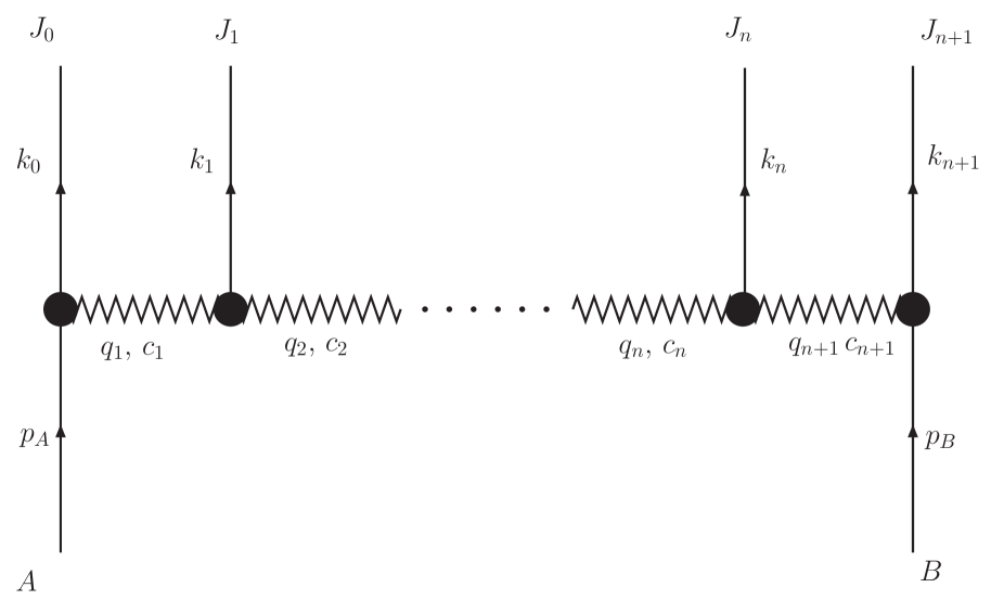
Figure 1: Schematic representation of the amplitude $2\rightarrow 2+n$. The zig-zag lines represent Reggeized gluon exchange. Right and left black blobs represent the Particle-Particle-Reggeon (PPR) vertices; black blobs in the middle represent the Reggeon-Reggeon-Particle vertices.

It is necessary to note here that the simple factorized form shown in Fig.1 is valid for the real parts of the MRK amplitudes only. In fact, the imaginary parts are much more complicated than the real ones and have not any factorized form at all.

In the following for any 4-vector $v$ we use the decomposition $v=v^{+}n_{1}+v^{-}n_{2}+v_{\perp}$ with light-cone vectors $n_{1,2}$ such that $(n_{1}n_{2})=1$, and therefore $v^{+}\equiv(v,n_{2}),\;\;v^{-}\equiv(v,n_{1})$. It is supposed that the dominant components of the momenta $p_{A}$ and $p_{B}$ of the initial particles $A$ and $B$ are $p^{+}_{A}$ and $p^{-}_{B}$ correspondingly, so that the squared energy in the c.m.s. $s\simeq 2p^{+}_{A}p^{-}_{B}$. Each of the final jets $J_{i},\;\;i=1,\ldots{n+1}$ with momentum $k_{i}=q_{i}-q_{i+1}\,\;\;q_{0}\equiv p_{A},\;\;q_{n+2}\equiv-p_{B}$ can represent either a single particle or a couple of particles. Their rapidities $y_{i}$, $y_{i}=\frac{1}{2}\ln\left(k^{+}_{i}/k^{-}_{i}\right)$ for $i=1,\ldots n$, $y_{0}=\ln\left(\sqrt{2}p^{+}_{A}/|q_{1\bot}|\right)$ and $y_{n+1}=\ln\left(|q_{(n+1)\bot}|/\sqrt{2}p^{-}_{B}\right)$ are strongly ordered: $y_{0}\gg y_{1}\gg\dots\gg y_{n}\gg y_{n+1}$; all $k_{i\perp}$ are limited.

In these denotations the multi-Regge form for the real parts of the MRK amplitudes can be written as

$$\Re{\cal A}_{2\rightarrow n+2}=2s\Gamma^{{R}_{1}}_{J_{0}A}\left(\prod_{i=1}^{n}\frac{e^{\omega(q_{i})(y_{i-1}-y_{i})}}{q^{2}_{i\perp}}\gamma^{J_{i}}_{{R}_{i}{R}_{i+1}}\right)\frac{e^{\omega(q_{n+1})(y_{n}-y_{n+1})}}{q^{2}_{(n+1)\perp}}\Gamma^{{R}_{n+1}}_{J_{n+1}B},$$ (2.1)

where $\omega(q)$ is called the gluon trajectory (in fact, the trajectory is $1+\omega(q)$), ${\Gamma}^{{R}}_{J_{0}A}$ and $\Gamma^{{R}}_{J_{n+1}B}$ are the scattering vertices and $\gamma^{J_{i}}_{{R}_{i}{R}_{i+1}}$ are the production vertices. The numerator of the Reggeon propagator ${e^{\omega(q_{i})(y_{i-1}-y_{i})}}=\Big{(}s_{i}/\sqrt{k^{2}_{i-1\perp}k^{2}_{i\perp}}\Big{)}^{\omega(q_{i})}$, where $s_{i}=(k_{i}+k_{i+1})^{2}\approx 2k^{-}_{i+1}k^{+}_{i}$ is known as the Regge-factor.

In the NLLA one has to know the gluon trajectory with the two-loop accuracy, the Reggeon vertices with one-particle jets with the one-loop corrections and the Reggeon vertices with two-particle jets at the Born approximation only. In QCD all these vertices and the trajectory were calculated with the required accuracy many years ago (see, for instance, [28] and references therein). Here we present them for a wide class of Yang-Mills theories with $n_{f}$ quark fields $\psi_{i}^{a_{i}}$ ($a_{i}$ and $i$ are correspondingly colour and flavour indices, $i=1,\dots,\,n_{f}$) and $n_{s}$ (pseudo)scalar fields $\phi_{r}^{A_{r}}$ ($A_{r}$ and $r$ are colour and flavour indices respectively, $r=1,\dots,\,n_{s}$) in any representations of the colour group with a general form of the Yukawa-type interaction

$${\cal L}_{Y}=g_{Y}\left(\bar{\psi}_{i}^{a_{i}}[\gamma_{5}]_{r}\psi_{j}^{c_{j}}\right)\;(R_{ij}^{r})_{a_{i}c_{j}}^{b_{r}}\;\phi_{r}^{b_{r}}+h.c.\,.$$ (2.2)

In the lagrangian (2.2) $[\gamma_{5}]_{r}=1$ for scalars and $[\gamma_{5}]_{r}=i\gamma_{5}=-\gamma^{0}\gamma^{1}\gamma^{2}\gamma^{3}$ for pseudoscalars; $(R_{ij}^{r})_{a_{i}c_{j}}^{b_{r}}$ are flavour matrices of the Yukawa-type interaction. Different fields transform according to different representations of the gauge group $SU(N_{c})$ with generators $T_{bc}^{a}=-if^{abc}$ for gluons, $t_{i}^{a}$ for quarks and ${\cal T}_{i}^{a}$ for scalars. The colour projectors $(R_{ij}^{r})_{a_{i}c_{j}}^{b_{r}}$ obey the commutation relations following from the gauge invariance:

$$(t_{f}^{a})_{c_{f}b}(R_{fi}^{r})_{bc_{i}}^{n_{r}}-(R_{fi}^{r})_{c_{f}d}^{n_{r}}(t_{i}^{a})_{dc_{i}}=(R_{fi}^{r})_{c_{f}c_{i}}^{m_{r}}({\cal T}^{a}_{r})_{m_{r}n_{r}}\,.$$ (2.3)

Here the summation is only performed over colour indices $b$, $d$, and $m_{r}$. We will use the symmetry factors $\kappa^{f}_{i}$ ($\kappa^{s}_{r}$) equal to ${1}/{2}$ for Majorana quarks (for the real scalars) and equal to 1 for Dirac quarks (for complex scalars) and the denotations

$$\xi_{f}=\sum_{i=1}^{n_{f}}\kappa^{f}_{i}\frac{T^{f}_{i}}{N_{c}}\,,\;\xi_{s}=\sum_{r=1}^{n_{s}}\kappa^{s}_{r}\frac{T^{s}_{r}}{N_{c}}\,,$$ (2.4)

where generators $T^{f}_{i},\;T^{s}_{r}$ are normalized by the relations

$$\mathrm{Tr}[T^{a}T^{b}]=N_{c}\delta_{ab}\,,\mathrm{Tr}[t_{i}^{a}t_{i}^{b}]=T^{f}_{i}\delta_{ab}\,,\;\mathrm{Tr}[{\cal T}_{r}^{a}{\cal T}_{r}^{b}]=T^{s}_{r}\delta_{ab}\,.$$ (2.5)

Quadratic Casimir operators are defined as

$$T^{a}T^{a}=C_{V}=N_{c},\;\;t^{a}_{i}t^{a}_{i}=C_{F}^{i}\,,\;{\cal T}_{r}^{a}{\cal T}_{r}^{a}=C_{S}^{r}.$$ (2.6)

In the fundamental representation $T^{f}_{i}=1/2$ and $C_{F}^{i}=(N_{c}^{2}-1)/(2N_{c})$. But note that we use the denotations $t^{a}_{i},T^{f}_{i}$ and $C_{F}^{i}$ for any representation of the colour group for quarks. The quark loop contributions with the colour structure $\mathrm{Tr}[t^{a}_{i}t^{b}_{i}]$ can be obtained from the QCD ones (where quarks are in the fundamental representation) by the substitution $n_{f}\rightarrow 2\sum_{i}\kappa^{f}_{i}T^{f}_{i}$, and the contributions with the colour structure $t^{a}_{i}t^{b}_{i}t^{a}_{i}$ by the substitution $1/N_{c}^{2}\rightarrow 1-2C_{F}^{i}/N_{c}$ . One can also restore the contributions of vacuum polarization by scalars from corresponding quark contribution in QCD by the substitution [30, 31] $n_{f}\rightarrow 2\sum_{r}\kappa^{s}_{r}T^{s}_{r}/(4(1+\epsilon))$.

It is worth noting that the interaction (2.2) permits transitions with nonconservation of fermion and scalar flavours. For the diagonal transitions we omit the flavour indices.

The $N$-extended SYM contains $n_{M}=N$ Majorana quarks and $n_{s}=2(N-1)$ neutral scalars. The matrices $(R_{if}^{r})_{a_{i}b_{f}}^{b_{r}}$ in SYM have the form $(R_{if}^{r})_{a_{i}b_{f}}^{b_{r}}=\Delta_{if}^{r}T_{a_{i}b_{f}}^{b_{r}}$ and the flavour matrices $\Delta^{r}$ subject to the conditions $[\Delta^{r}]^{2}=-1$, $\mathrm{Tr}[\Delta^{r}]=0$, $\mathrm{Tr}[\Delta^{r}\Delta^{t}]=n_{f}\delta^{rt}$ with $n_{f}=n_{M}$. The Yukawa constant in SYM reduces to $g_{Y}=g/2$.

As it is known, dimensional regularization violates supersymmetry, therefore in SYM a modification of the dimensional regularization is used which is called dimensional reduction  [32]. Hereafter to present explicitly $N=4$ SYM results we use the dimensional reduction scheme, where $n_{s}=6-2\epsilon$.

3 Gluon Regge trajectory and Reggeon vertices

Apart from contributions of the Yukawa-type interaction (2.2), all Reggeon vertices as well as the gluon trajectory in the Yang-Mills theories with quarks and scalars in any representations of the colour group can be obtained from known results with the NLLA accuracy by the substitutions discussed above.

There are two kinds of scattering vertices: with dominant $+$ and dominant $-$ components of particle momenta, or, in other words, in fragmentation region of particles $A$ and $B$. Evidently, ones can be obtained from other by appropriate substitutions. We present the scattering vertices for the particle $A$ fragmentation region.

3.1 Gluon trajectory

The two-loop calculations of the trajectory were carried out in Refs. [33, 34, 35, 36, 37] and then confirmed in [38, 39]. Using the integral representation for the trajectory in QCD [34] we obtain in $D=4+2\epsilon$ space time dimensions

$$\omega(-\vec{q}_{i}^{\;2})=\frac{-\bar{g}^{2}\;\vec{q}_{i}^{\;2}}{\pi^{1+\epsilon}\Gamma(1-\epsilon)}\int\frac{d^{2+2\epsilon}k\;}{\vec{k}^{\;2}(\vec{k}-\vec{q}_{i})^{2}}\Biggl{(}1+\bar{g}^{2}\Biggl{[}f(\vec{k},0)+f(0,\vec{k}-\vec{q}_{i})-f(\vec{k},\vec{k}-\vec{q}_{i})\Biggr{]}\Biggr{)}~{},$$ (3.1)

where

$$\bar{g}^{2}=\frac{g^{2}N_{c}\Gamma(1-\epsilon)}{(4\pi)^{2+{\epsilon}}}~{},$$ (3.2)

$\Gamma(x)$ is the Euler gamma-function, $g$ is the bare coupling, and

$$f(\vec{k}_{1},\vec{k}_{2})=\frac{(\vec{k}_{1}-\vec{k}_{2})^{2}}{\pi^{1+\epsilon}\Gamma(1-\epsilon)}\int\frac{d^{2+2\epsilon}l}{(\vec{k}_{1}-\vec{l})^{2}(\vec{k}_{2}-\vec{l})^{2}}\Biggl{(}\ln\left(\frac{(\vec{k}_{1}-\vec{k}_{2})^{2}}{\vec{l}^{\;2}}\right)-2\psi(1+2\epsilon)-\psi\left(1-\epsilon\right)$$

$$+2\psi\left(1+\epsilon\right)+\psi(1)-\frac{1}{\epsilon}-\frac{a_{1}}{2(1+2\epsilon)(3+2\epsilon)}\Biggr{)}~{},$$ (3.3)

$$\psi(x)=\frac{\Gamma^{\prime}(x)}{\Gamma(x)},\;\;a_{1}=11+7\epsilon-4(1+\epsilon)\xi_{f}-\xi_{s}.$$ (3.4)

For $N=4$ SYM, the coefficients $a_{1}$ vanishes in the dimensional reduction.

An explicit expression for the trajectory was calculated in QCD [37] only the limit $\epsilon\rightarrow 0$. Using this result we obtain

$$\omega(-\vec{q}^{\;2})=-\bar{g}^{2}(\vec{q}^{\;2})^{\epsilon}\frac{\Gamma^{2}(\epsilon)}{\Gamma(2\epsilon)}+\bar{g}^{4}(\vec{q}^{\;2})^{2\epsilon}\left[a_{1}\left(\frac{1}{3\epsilon^{2}}-\frac{8}{9\epsilon}+\frac{52}{27}\right)+\frac{2}{\epsilon}\zeta(2)-2\zeta(3)+{\cal O}(\epsilon)\right],$$ (3.5)

where $\zeta(n)$ is the Riemann zeta-function. In $N=4$ SYM with the dimensional reduction one has

$$\omega(-\vec{q}^{\;2})_{N=4SYM}=-\bar{g}^{2}(\vec{q}^{\;2})^{\epsilon}\frac{\Gamma^{2}(\epsilon)}{\Gamma(2\epsilon)}+\bar{g}^{4}(\vec{q}^{\;2})^{2\epsilon}\left[\frac{2}{\epsilon}\zeta(2)-2\zeta(3)+{\cal O}(\epsilon)\right]~{}.$$ (3.6)

In the ${\overline{\mbox{MS}}}$ scheme the bare coupling is connected to the renormalized coupling, $g_{\mu}$, through the relation

$$g=g_{\mu}\mu^{-\mbox{\normalsize$\epsilon$}}\left[1+\bar{g}_{\mu}^{2}\frac{\beta_{0}}{2N_{c}\epsilon}\right]~{},\;\;\bar{g}_{\mu}^{2}=\frac{g_{\mu}^{2}N_{c}\Gamma(1-\epsilon)}{(4\pi)^{2+{\epsilon}}}~{},\;\;\frac{\beta_{0}}{N_{c}}=\frac{11}{3}-\frac{4}{3}\xi_{f}-\frac{1}{3}\xi_{s}~{}.$$ (3.7)

In terms of the renormalized coupling, one obtains

$$\omega(-\vec{q}^{\;2})=-\bar{g}^{2}_{\mu}\left(\frac{\vec{q}^{\;2}}{\mu^{2}}\right)^{\epsilon}\frac{\Gamma^{2}(\epsilon)}{\Gamma(2\epsilon)}-\bar{g}^{4}_{\mu}\left(\frac{\vec{q}^{\;2}}{\mu^{2}}\right)^{2\epsilon}\left[\frac{\beta_{0}}{N_{c}}\left(\frac{1}{\epsilon^{2}}-\ln^{2}\left(\frac{\vec{q}^{\;2}}{\mu^{2}}\right)\right)+\left(\frac{1}{\epsilon}+2\ln\left(\frac{\vec{q}^{\;2}}{\mu^{2}}\right)\right)\right.$$

$$\left.\times\left(\frac{67}{9}-2\zeta(2)-\frac{20}{9}\xi_{f}-\frac{8}{9}\xi_{s}\right)-\frac{404}{27}+2\zeta(3)+\frac{112}{27}\xi_{f}+\frac{52}{27}\xi_{s}+{\cal O}(\epsilon)\right].$$ (3.8)

3.2 Vertices for one-particle jets

Reggeon vertices with gluons are gauge invariant. To simplify representation of these vertices, we will use for the polarization vector $e$ of the gluon with the momentum $k$ the light-cone gauge $(en_{2})=0$, so that

$$e^{\mu}=e^{\mu}_{\perp}-\frac{(e,k)_{\perp}}{kn_{2}}n_{2}^{\mu}~{}.$$ (3.9)

It worth noting that knowing some vertex in this gauge, one can restore its gauge invariant form. Here we have used the notation $(a,b)_{\bot}\equiv(a_{\bot},b_{\bot})$.

Scattering vertices

Using results of Refs. [40, 34, 41, 42] for the one-loop gluon, quark and scalar corrections correspondingly, we obtain for the gluon-gluon-Reggeon vertex $\Gamma_{G^{\prime}G}^{R}$

$$\Gamma_{G^{\prime}G}^{R}=-g\bigl{(}e^{{}^{\prime}*},e\bigr{)}_{\bot}T_{G^{\prime}G}^{R}\Biggl{[}1-\bar{g}^{2}(-q_{\bot}^{2})^{\epsilon}\frac{\Gamma^{2}(1+\epsilon)}{\epsilon\Gamma(1+2\epsilon)}\biggl{(}\frac{2}{\epsilon}+\psi(1)+\psi(1-\epsilon)-2\psi(1+\epsilon)-$$

$$-\frac{(1+\epsilon)^{2}a_{1}+2\epsilon^{2}a_{2}}{2(1+\epsilon)^{2}(1+2\epsilon)(3+2\epsilon)}\biggr{)}\Biggr{]}-2g\bar{g}^{2}(-q_{\bot}^{2})^{\epsilon}\frac{\Gamma^{2}(1+\epsilon)}{(1+\epsilon)\Gamma(4+2\epsilon)}$$

$$\times T_{G^{\prime}G}^{R}e_{\bot\mu}^{{}^{\prime}*}e_{\bot\nu}\biggl{(}g_{\bot}^{\mu\nu}-(D-2)\frac{q_{\bot}^{\mu}q_{\bot}^{\nu}}{q_{\bot}^{2}}\biggr{)}a_{2},$$ (3.10)

where $e$ and $e^{\prime}$ are the polarization vectors of the gluons $G$ and $G^{\prime}$ respectively, $q$ is the Reggeon momentum, $T_{G^{\prime}G}^{R}$ is the colour factor,

$$a_{2}=1+\epsilon-2\xi_{f}+\xi_{s}.$$ (3.11)

For $N=4$ SYM, the coefficients $a_{2}$ vanishes in the dimensional reduction.

The quark-quark-Reggeon vertex $\Gamma_{Q^{\prime}Q}^{R}$ with one-loop accuracy was calculated in QCD in [43]. Scalar corrections in SYM were found in [42]. Using these results, we obtain

$$\Gamma_{Q^{\prime}_{f}Q_{i}}^{R}=g\delta_{fi}\bar{u}_{f}(p^{\prime})t_{i}^{R}\frac{n\mspace{-8.0mu}/_{2}}{2p^{+}}u_{i}(p)\biggl{[}1-\bar{g}^{2}(-q_{\bot}^{2})^{\epsilon}\frac{\Gamma^{2}(1+\epsilon)}{\epsilon\Gamma(1+2\epsilon)}\biggl{(}\frac{1}{\epsilon}+\psi(1-\epsilon)+\psi(1)-2\psi(1+\epsilon)$$

$$+\frac{a_{1}-3(3+2\epsilon)}{2(1+2\epsilon)(3+2\epsilon)}+\Bigl{(}\frac{2C_{F}^{i}}{N_{c}}-1\Bigr{)}\Bigl{(}\frac{1}{\epsilon}-\frac{3-2\epsilon}{2(1+2\epsilon)}\Bigr{)}\biggr{)}\biggr{]}+\Gamma_{Q^{\prime}_{f}Q_{i}}^{R(Y)}\,,$$ (3.12)

where $\Gamma_{Q^{\prime}_{f}Q_{i}}^{R(Y)}$ is the contribution of the Yukawa-type interaction. We don’t present it here in the general case because we don’t need its explicit form to prove the validity of the bootstrap conditions. In SYM this term is absent due to the cancellation of the scalar and pseudoscalar contributions. They have different signs because corresponding matrix elements contain odd numbers of gamma matrices between two matrices $\gamma_{5}$ in the pseudoscalar case and two identity matrices in the scalar case.

The scalar-scalar-Reggeon vertex $\Gamma_{S^{\prime}_{r^{\prime}}S_{r}}^{R}$ was calculated in [42] in SYM by the method developed in [44]. The calculations can be easily extended to any representation of the colour group with the result

$$\begin{split}&\Gamma_{S^{\prime}_{r^{\prime}}S_{r}}^{R}=g\delta_{r^{\prime}r}({\cal T}_{r}^{R})_{S^{\prime}_{r^{\prime}}S_{r}}\Biggl{[}1-\bar{g}^{2}(-q_{\bot}^{2})^{\epsilon}\frac{\Gamma^{2}(1+\epsilon)}{\epsilon\Gamma(1+2\epsilon)}\biggl{(}\frac{1}{\epsilon}+\psi(1-\epsilon)+\psi(1)-2\psi(1+\epsilon)+\\ &+\frac{a_{1}-4(3+2\epsilon)}{2(1+2\epsilon)(3+2\epsilon)}+\Bigl{(}\frac{2C_{S}^{r}}{N_{c}}-1\Bigr{)}\biggl{[}\frac{1}{\epsilon}-\frac{2}{1+2\epsilon}\biggr{]}\biggl{)}\Biggl{]}+\Gamma_{S^{\prime}_{r^{\prime}}S_{r}}^{R(Y)}\,,\end{split}$$ (3.13)

where $\Gamma_{S^{\prime}_{r^{\prime}}S_{r}}^{R(Y)}$ is the contribution of the Yukawa-type interaction. As well as for the quark vertex, we don’t present it here in the general case, because we don’t need its explicit form. In SYM we have [42]

$$\Gamma_{S^{\prime}S}^{R(Y)}=-gT_{S^{\prime}S}^{R}\bar{g}^{2}(-q_{\bot}^{2})^{\epsilon}\frac{\Gamma^{2}(1+\epsilon)}{\epsilon\Gamma(1+2\epsilon)}\;2\xi_{f}\frac{(-1)^{I_{s}}}{1+2\epsilon}\;,$$ (3.14)

where $I_{s}=0$ if $S$ is a scalar and $I_{s}=1$ if $S$ is a pseudoscalar.

Production vertex

In the Born approximation the Reggeon-Reggeon-gluon vertex $\gamma_{R_{1}R_{2}}^{G}$ was obtained in [5]. One-loop gluon corrections to the vertex were calculated in Refs. [40, 45, 46, 47]. In the last paper they were obtained at arbitrary $D=4+2\epsilon$. With the same accuracy, the quark and scalar corrections were obtained in [48] and [31] respectively. At arbitrary $D$ the corrections are rather complicated (mainly because of the gluon contribution). We present them here in the form where only terms singular at small gluon transverse momentum $\vec{k}$ ($k=q_{1}-q_{2},\;q_{1,2}$ are the momenta of the Reggeons $R_{1,2}$) are given at arbitrary D, but the other terms in the limit $\epsilon\rightarrow 0$.

$$\begin{split}&\gamma_{R_{1}R_{2}}^{G}=\gamma_{R_{1}R_{2}}^{G(B)}+2g\bar{g}^{2}T_{R_{1}R_{2}}^{G}e_{\bot\mu}^{*}(k)q_{1\bot}^{2}V^{\mu}(q_{1},q_{2})~{},\end{split}$$ (3.15)

where

$$\gamma_{R_{1}R_{2}}^{G(B)}=-2gT_{R_{1}R_{2}}^{G}e_{\bot\mu}^{*}\biggl{(}{q_{1\bot}^{\mu}}-k_{\bot}^{\mu}\frac{q_{1\bot}^{2}}{k_{\bot}^{2}}\biggr{)}$$ (3.16)

is the Born vertex [5] in the light-cone gauge $(e,n_{2})=0$,

$$V^{\mu}(q_{1},q_{2})=\Bigl{(}\frac{11}{6}-\frac{2\xi_{f}}{3}-\frac{\xi_{s}}{6}\Bigr{)}\Biggl{(}\frac{k^{\mu}_{\bot}}{k_{\bot}^{2}}-\frac{q_{1\bot}^{\mu}}{q_{1\bot}^{2}}\frac{q_{1\bot}^{2}+q_{2\bot}^{2}}{q_{1\bot}^{2}-q_{2\bot}^{2}}\Biggr{)}\ln\frac{q_{1\bot}^{2}}{q_{2\bot}^{2}}+\Bigl{(}\frac{1}{6}-\frac{\xi_{f}}{3}+\frac{\xi_{s}}{6}\Bigr{)}$$

$$\times\Biggl{[}\Biggl{(}\biggl{(}\frac{k^{\mu}_{\bot}}{k_{\bot}^{2}}-\frac{q_{1\bot}^{\mu}}{q_{1\bot}^{2}}\biggr{)}\frac{2k_{\bot}^{2}}{\bigl{(}q_{1\bot}^{2}-q_{2\bot}^{2}\bigr{)}^{2}}+\frac{k_{\bot}^{\mu}\bigl{(}2k_{\bot}^{2}-q_{1\bot}^{2}-q_{2\bot}^{2}\bigr{)}}{q_{1\bot}^{2}\bigl{(}q_{1\bot}^{2}-q_{2\bot}^{2}\bigr{)}^{2}}\biggr{)}\Bigl{[}q_{1\bot}^{2}+q_{2\bot}^{2}-\frac{2q_{1\bot}^{2}q_{2\bot}^{2}}{q_{1\bot}^{2}-q_{2\bot}^{2}}\ln\frac{q_{1\bot}^{2}}{q_{2\bot}^{2}}\Bigr{]}-\frac{k_{\bot}^{\mu}}{q_{1\bot}^{2}}\Biggr{]}$$

$$-\frac{1}{2}\biggl{(}\frac{k^{\mu}_{\bot}}{k_{\bot}^{2}}-\frac{q_{1\bot}^{\mu}}{q_{1\bot}^{2}}\biggr{)}\biggl{(}\ln^{2}\frac{q_{1\bot}^{2}}{q_{2\bot}^{2}}+\frac{2\bigl{|}k_{\bot}^{2}\bigr{|}^{\epsilon}}{\epsilon^{2}}-{\pi^{2}}\biggr{)}~{}.$$ (3.17)

For $N=4$ SYM in the dimensional reduction scheme

$$\gamma_{R_{1}R_{2}}^{G}=\gamma_{R_{1}R_{2}}^{G(B)}\biggl{(}1-\bar{g}^{2}\biggl{[}\frac{[-k_{\bot}^{2}]^{\epsilon}}{\epsilon^{2}}-\frac{\pi^{2}}{2}+\frac{1}{2}\ln^{2}\Big{[}\frac{q_{1\bot}^{2}}{q_{2\bot}^{2}}\Big{]}\biggr{]}\biggr{)}.$$ (3.18)

3.3 Vertices for two-particle jets

Now we turn to vertices which are absent in the LLA and appear in the NLLA. They are needed in the Born approximation only.

Scattering vertices

We will present the vertices $\Gamma_{JP}^{R}$ of the transition of a particle $P$ to a two-particle jet $J$. The vertex of the inverse transition $\Gamma_{PJ}^{R}=\left(\Gamma_{JP}^{R}\right)^{*}$. We denote the momentum of the initial particle $k$ and the momenta of the final particles $l_{1},\,l_{2}$, total jet momentum is $l=l_{1}+l_{2},\;l^{+}=k^{+}$ (remind, we are in the particle $A$ fragmentation region),

$$k=k^{+}n_{1}-\frac{k_{\bot}^{2}}{2k^{+}}n_{2}+k_{\bot}\,,\quad l_{i}=x_{i}l^{+}n_{1}-\frac{l_{i\bot}^{2}}{2x_{i}l^{+}}n_{2}+l_{i\bot},\;i=1,\,2,\;x_{1}+x_{2}=1.$$ (3.19)

The vertex of quark $\rightarrow$ quark-gluon jet transition $\Gamma_{\{QG\}Q}^{R}$ has the same form as in QCD [35, 49]. It can also be written as in [50]:

$$\begin{split}&\Gamma_{\{QG\}Q}^{R}=g^{2}e^{*}_{\bot\mu}\bar{u}(l_{1})\frac{n\mspace{-8.0mu}/_{2}}{2k^{+}}\Bigl{[}t^{G}_{i}t^{R}_{i}\bigl{(}{\cal A}^{\mu}_{b}(x_{2}l_{1\perp}-x_{1}l_{2\perp})-{\cal A}^{\mu}_{b}(l_{1\perp}-x_{1}k_{\perp})\bigr{)}\\ &-t^{R}_{i}t^{G}_{i}\bigl{(}{\cal A}^{\mu}_{b}(-l_{2\perp}+x_{2}k_{\perp})-{\cal A}^{\mu}_{b}(l_{1\perp}-x_{1}k_{\perp})\bigr{)}\Bigr{]}u(k)~{},\end{split}$$ (3.20)

where $e$ is the gluon polarization vector, quark colour and flavour wave functions are included in $\bar{u}(l_{1})$ and $u(k)$,

$${\cal A}^{\mu}_{b}(p)=-\frac{1}{p^{2}}\left(x_{1}\gamma^{\mu}{p\mspace{-8.0mu}/}+{p\mspace{-8.0mu}/\gamma^{\mu}}\right)~{}.$$ (3.21)

Let us present the vertices of the gluon $G$ transition to pairs $\{P_{1}(l_{1}),\bar{P}_{2}(l_{2})\}$ in the form

$$\Gamma_{\{P_{1}\bar{P}_{2}\}G}^{R}=g^{2}e_{\bot\mu}\bigl{(}\textbf{T}^{G}\textbf{T}^{R}A^{\mu}_{P_{1}P_{2}}(k)+\textbf{T}^{R}\textbf{T}^{G}A^{\mu}_{P_{2}P_{1}}(k)\bigr{)}\,,$$ (3.22)

where ${\mathbf{T}}^{R}$ are the colour group generators for produced particles in the corresponding representation. Generators $\Big{(}\textbf{T}^{R}\textbf{T}^{G}\Big{)}_{P_{1}P_{2}}$ and $\Big{(}\textbf{T}^{G}\textbf{T}^{R}\Big{)}_{P_{1}P_{2}}$ operate with the colour wave functions of the particle produced in (3.22).

For gluon $\rightarrow$ quark-antiquark transition one has

$$A^{\mu}_{Q\bar{Q}}(k)=\bar{u}(l_{1})\frac{n\mspace{-8.0mu}/_{2}}{2k^{+}}\bigl{(}{\cal A}^{\mu}_{p}(l_{1\perp}-x_{1}k_{\perp})-{\cal A}^{\mu}_{p}(x_{2}l_{1\perp}-x_{1}l_{2\perp})\bigr{)}v(l_{2})~{},$$ (3.23)

with

$${\cal A}^{\mu}_{p}(p)=\frac{1}{p^{2}}\left(x_{1}\gamma^{\mu}{p\mspace{-8.0mu}/}-x_{2}{p\mspace{-8.0mu}/\gamma^{\mu}}\right)~{}.$$ (3.24)

The second term in (3.22) reads as follows (the minus sign is associated with Fermi statistics)

$$A^{\mu}_{\bar{Q}Q}(k)=-A^{\mu}_{Q\bar{Q}}(k)\Bigl{|}_{l_{1}\leftrightarrow l_{2}}=-\bar{u}(l_{1})\frac{n\mspace{-8.0mu}/_{2}}{2k^{+}}\bigl{(}{\cal A}^{\mu}_{p}(-l_{2\perp}+x_{2}k_{\perp})-{\cal A}^{\mu}_{p}(x_{2}l_{1\perp}-x_{1}l_{2\perp})\bigr{)}v(l_{2})~{}.$$ (3.25)

Let us note that the vertex $\Gamma_{\{Q\bar{Q}\}G}^{R}$ [51] can be obtained from $\Gamma_{\{QG\}Q}^{R}$ by crossing, i.e. by the replacement

$$x_{2}\rightarrow\frac{1}{x_{2}},\;x_{1}\rightarrow-\frac{x_{1}}{x_{2}},\;l_{2\bot}\leftrightarrow-k_{\bot},\;e^{*}_{\bot\mu}\rightarrow e_{\bot\mu},\;u(k)\rightarrow v(l_{2})~{}.$$ (3.26)

The gauge invariant gluon $\rightarrow$ gluon-gluon jet Reggeon vertex $\Gamma_{\{G_{1}G_{2}\}G}^{R}$ was obtained in [52]. In the light-cone gauge we have [51] for the representation (3.22):

$$A^{\mu}_{G_{1}G_{2}}(k)=2e^{*\nu}_{1\bot}e^{*\rho}_{2\bot}\bigl{(}{\cal A}_{\mu\nu\rho}(l_{1\bot}-x_{1}k_{\bot})-{\cal A}_{\mu\nu\rho}(x_{2}l_{1\bot}-x_{1}l_{2\bot})\bigr{)}~{},$$ (3.27)

where $e_{1,2}$ are the polarization vectors of the gluons $G_{1,2}$ with the momenta $l_{1,2}$, and

$${\cal A}_{\mu\nu\rho}(p)=\frac{1}{p^{2}}\bigl{(}x_{1}x_{2}g^{\nu\rho}p^{\mu}-x_{1}g^{\mu\nu}p^{\rho}-x_{2}g^{\mu\rho}p^{\nu}\bigr{)}~{}.$$ (3.28)

For the vertex of the scalar pair $\{S(l_{1}),\,\bar{S}(l_{2})\}$ production by the gluon $G(k)$ [42] we have in (3.22)

$$A^{\mu}_{S\bar{S}}(k)=-2\Big{(}M_{p}^{\mu}(l_{1\bot}-x_{1}k_{\bot})-M_{p}^{\mu}(x_{2}l_{1\bot}-x_{1}l_{2\bot})\Big{)}~{},$$ (3.29)

where

$$M_{p}^{\mu}(p)=x_{1}x_{2}\frac{p^{\mu}}{p^{2}}~{}.$$ (3.30)

The scalar $\rightarrow$ scalar-gluon jet vertex can be easily obtained from the previous one by the crossing replacement (3.26):

$$\Gamma_{\{GS^{\prime}\}S}^{R}=-2g^{2}e_{\bot\mu}^{*}\biggl{[}\Big{(}{\cal T}^{G}_{r}{\cal T}^{R}_{r}\Big{)}_{S^{\prime}S}\Big{(}M_{b}^{\mu}(x_{2}l_{1}-x_{1}l_{2})-M_{b}^{\mu}(l_{1}-x_{1}k)\Big{)}$$ (3.31)

$$-\Big{(}{\cal T}^{R}_{r}{\cal T}^{G}_{r}\Big{)}_{S^{\prime}S}\Big{(}M_{b}^{\mu}(-l_{2}+x_{2}k)-M_{b}^{\mu}(l_{1}-x_{1}k)\Big{)}\biggr{]},\;M_{b}^{\mu}(p)=x_{1}\frac{p_{\bot}^{\mu}}{p_{\bot}^{2}}\,.$$

The rest particle $\rightarrow$ two-particle jet transitions exist due to Yukawa-type interaction. The Reggeon vertices for these transitions in SYM were calculated in [42]. The scalar $\rightarrow$ quark-antiquark vertex is written as

$$\begin{split}\Gamma_{\{Q_{i}\bar{Q}_{j}\}S_{r}}^{R}&=-gg_{Y}\bar{u}_{i}(l_{1})\frac{n\mspace{-8.0mu}/_{2}}{2k^{+}}\Biggl{[}t^{R}_{i}(R_{ij}^{r})^{S_{r}}\biggl{(}\frac{(x_{2}l\mspace{-8.0mu}/_{1}-x_{1}l\mspace{-8.0mu}/_{2})_{\bot}}{(x_{2}l_{1}-x_{1}l_{2})_{\bot}^{2}}+\frac{(l\mspace{-8.0mu}/_{2}-x_{2}k\mspace{-8.0mu}/)_{\bot}}{(l_{2}-x_{2}k)_{\bot}^{2}}\biggr{)}+\\ +&(R_{ij}^{r})^{S_{r}}t_{j}^{R}\biggl{(}\frac{(x_{1}l\mspace{-8.0mu}/_{2}-x_{2}l\mspace{-8.0mu}/_{1})_{\bot}}{(x_{2}l_{1}-x_{1}l_{2})_{\bot}^{2}}+\frac{(l\mspace{-8.0mu}/_{1}-x_{1}k\mspace{-8.0mu}/)_{\bot}}{(l_{1}-x_{1}k)_{\bot}^{2}}\biggr{)}\Biggr{]}[\gamma_{5}]_{r}v_{j}(l_{2})\,,\end{split}$$ (3.32)

where $i$ is quark and $j$ is and anti-quark flavour, $r$ is the scalar flavour ($S_{r}$ is the scalar colour index); $[\gamma_{5}]_{r}=1$ if $S$ is the scalar, and $[\gamma_{5}]_{r}=i\gamma_{5}$ for the pseudoscalar case. The crossing vertex $\Gamma_{\{Q^{\prime}(l_{1})S(l_{2})\}Q(k)}^{R}$ is

$$\Gamma_{\{Q^{\prime}_{i}S_{r}\}Q_{j}}^{R} =-gg_{Y}\bar{u}_{i}(l_{1})\frac{n\mspace{-8.0mu}/_{2}}{2k^{+}}x_{2}\biggl{[}t^{R}_{i}\Bigl{[}(R_{ji}^{r})^{S_{r}}\Bigr{]}^{{\dagger}}\biggl{(}\frac{(l\mspace{-8.0mu}/_{1}-x_{1}k\mspace{-8.0mu}/)_{\bot}}{(l_{1}-x_{1}k)_{\bot}^{2}}+\frac{(l_{2}\mspace{-8.0mu}/-x_{2}k\mspace{-8.0mu}/)_{\bot}}{(l_{2}-x_{2}k)_{\bot}^{2}}\biggr{)}+$$ (3.33)

$$+ \Bigl{[}(R_{ji}^{r})^{S_{r}}\Bigr{]}^{{\dagger}}t^{R}_{j}\biggl{(}\frac{(x_{2}l\mspace{-8.0mu}/_{1}-x_{1}l\mspace{-8.0mu}/_{2})_{\bot}}{(x_{2}l_{1}-x_{1}l_{2})_{\bot}^{2}}-\frac{(l\mspace{-8.0mu}/_{1}-x_{1}k\mspace{-8.0mu}/)_{\bot}}{(l_{1}-x_{1}k)_{\bot}^{2}}\biggr{)}\biggr{]}[\gamma_{5}]_{r}u_{j}(k)\,.$$

Production vertices

Denoting momenta of produced particles $P_{1}$ and $P_{2}$ as $l_{1}$ and $l_{2}$, of Reggeons $R_{1},\,R_{2}$ momenta as $q_{1}$ and $q_{2}$, $q_{1}-q_{2}=l_{1}+l_{2}=l$, we have for the jet production vertices:

$$\gamma_{R_{1}R_{2}}^{\{P_{1}P_{2}\}}=g^{2}\bigl{(}\textbf{T}^{R_{1}}\textbf{T}^{R_{2}}B_{P_{1}P_{2}}(q_{1};l_{1},l_{2})+\textbf{T}^{R_{2}}\textbf{T}^{R_{1}}B_{P_{2}P_{1}}(q_{1};l_{2},l_{1})\bigr{)}\,,$$ (3.34)

where ${\mathbf{T}}^{R}$ are the colour group generators for produced particles. Here for quark-antiquark production $\{Q(l_{1}),\bar{Q}(l_{2})\}$ one has [53, 54, 55]

$$\begin{split}&B_{Q\bar{Q}}(q_{1};l_{1},l_{2})=\bar{u}(l_{1})\frac{n\mspace{-8.0mu}/_{2}}{l^{+}}b(q_{1};l_{1},l_{2})v(l_{2})~{},\\ &\;B_{\bar{Q}Q}(q_{1};l_{2},l_{1})=-B_{Q\bar{Q}}(q_{1};l_{1},l_{2})\Bigl{|}_{l_{1}\leftrightarrow l_{2}}=-\bar{u}(l_{1})\frac{n\mspace{-8.0mu}/_{2}}{l^{+}}\overline{b(q_{1};l_{2},l_{1})}v(l_{2})\,,\end{split}$$ (3.35)

where

$$\begin{split}&b(q_{1};l_{1},l_{2})=\frac{l\!\!\!/_{1\bot}(l\!\!\!/_{1\bot}-q\!\!\!/_{1\bot})}{x_{1}(q_{1}-l_{1})_{\bot}^{2}+x_{2}l_{1\bot}^{2}}+\frac{x_{1}x_{2}}{\Lambda^{2}_{\bot}}\biggl{[}\frac{q_{1\bot}^{2}\bigl{(}l\!\!\!/_{1\bot}\Lambda\!\!\!/_{\bot}-\Lambda\!\!\!/_{\bot}l\!\!\!/_{2\bot}\bigr{)}}{\Lambda_{\bot}^{2}+x_{1}x_{2}l_{\bot}^{2}}+\frac{\Lambda\!\!\!/_{\bot}q\!\!\!/_{1\bot}}{x_{1}}-\frac{q\!\!\!/_{1\bot}\Lambda\!\!\!/_{\bot}}{x_{2}}\biggr{]}-1~{},\\ &\overline{b(q_{1};l_{1},l_{2})}=\gamma^{0}b^{{\dagger}}(q_{1};l_{1},l_{2})\gamma^{0}\,,\qquad\Lambda_{\bot}^{\mu}=\bigl{(}x_{2}l_{1}-x_{1}l_{2}\bigr{)}^{\mu}_{\bot}\,.\end{split}$$ (3.36)

For the vertex of two-gluon $\{G_{1}(l_{1}),G_{2}(l_{2})\}$ production the result was obtained in the gauge invariant form [52]. In the light-cone gauge (3.9) it reads as [56]:

$$\begin{split}&B_{G_{1}G_{2}}(q_{1};l_{1},l_{2})=4e^{*\alpha}_{1\bot}e^{*\beta}_{2\bot}\Biggl{(}\frac{1}{2}g^{\alpha\beta}_{\bot}\Biggl{[}\frac{x_{1}x_{2}}{\Lambda_{\bot}^{2}}\Bigl{(}-2(q_{1\bot},\Lambda_{\bot})+q_{1\bot}^{2}\frac{\left(\Lambda_{\bot},x_{2}l_{1\bot}+x_{1}l_{2\bot}\right)}{x_{2}l^{2}_{1\bot}+x_{1}l^{2}_{2\bot}}\Biggr{)}\\ &-x_{1}x_{2}\frac{q_{1\bot}^{2}-2(q_{1\bot},l_{1\bot})}{x_{1}(q_{1}-l_{1})^{2}_{\bot}+x_{2}l_{1\bot}^{2}}\Biggr{]}-\frac{x_{2}l_{1\bot}^{\alpha}q_{1\bot}^{\beta}-x_{1}q_{1\bot}^{\alpha}(q_{1}-l_{1})_{\bot}^{\beta}}{x_{1}(q_{1}-l_{1})^{2}_{\bot}+x_{2}l_{1\bot}^{2}}-\frac{x_{1}q_{1\bot}^{2}l_{1\bot}^{\alpha}(q_{1}-l_{1})^{\beta}_{\bot}}{l_{1\bot}^{2}(x_{1}(q_{1}-l_{1})^{2}_{\bot}+x_{2}l_{1\bot}^{2})}\\ &+\frac{x_{1}q_{1\bot}^{\alpha}\Lambda_{\bot}^{\beta}+x_{2}q_{1\bot}^{\beta}\Lambda_{\bot}^{\alpha}}{\Lambda_{\bot}^{2}}+\frac{x_{1}q_{1\bot}^{2}l_{1\bot}^{\alpha}l_{2\bot}^{\beta}}{l_{1\bot}^{2}(x_{2}l^{2}_{1\bot}+x_{1}l^{2}_{2\bot})}-\frac{x_{1}x_{2}q_{1\bot}^{2}}{\Lambda_{\bot}^{2}(x_{2}l^{2}_{1\bot}+x_{1}l^{2}_{2\bot})}\Bigl{(}\Lambda_{\bot}^{\alpha}l_{2\bot}^{\beta}+l_{1\bot}^{\alpha}\Lambda_{\bot}^{\beta}\Bigr{)}\Biggr{)}\,.\end{split}$$ (3.37)

For the vertex of two scalar $\{S(l_{1})\bar{S}(l_{2})\}$ production one has [31]:

$$B_{S\bar{S}}(q_{1};l_{1},l_{2})=2q^{2}_{1\perp}x_{1}x_{2}\Bigg{\{}\Bigg{[}\frac{x_{2}-x_{1}}{(l_{1}-x_{1}q_{1})^{2}_{\perp}+x_{1}x_{2}q^{2}_{1\perp}}+2\frac{(q_{1},\Lambda)_{\perp}}{q^{2}_{1\perp}\Lambda^{2}_{\perp}}-$$ (3.38)

$$-2\frac{(q_{1},l_{1}-x_{1}q_{1})_{\perp}}{q^{2}_{1\perp}[(l_{1}-x_{1}q_{1})^{2}_{\perp}+x_{1}x_{2}q^{2}_{1\perp}]}\Bigg{]}-\Bigg{[}q_{1}\rightarrow l\Bigg{]}\Bigg{\}}.$$

4 Bootstrap approach to the proof of the multi-Regge amplitude form

4.1 Bootstrap relations

In QCD, the scheme of the proof was formulated in [29]. The main point of the scheme is use of the restrictions imposed on the amplitudes with negative signatures in all $t_{i}$-channels by the unitarity conditions.

Signature (positive or negative) is a quantum number attributed to Reggeons in the theory of complex angular momenta. Amplitudes with Reggeon exchanges have corresponding signatures. At high energy it means the corresponding symmetry with respect to the sign change of the energy variables. The signature of the Reggeized gluon is negative, i.e. the MRK amplitudes with the Reggeized gluon exchange in the channel $t_{i}$ are odd with respect to the replacements $s_{jk}\rightarrow-s_{jk},\;(s_{jk})=(k_{i}+k_{j})^{2}$ for $k\geq i\geq j+1$. For the MRK amplitudes in the Born approximation this property is fulfilled for any $t_{i}$ thanks to the common factor $s$. Therefore the Born amplitudes have negative signatures in all $t_{i}$–channels and can be considered as amplitudes with Reggeized gluon exchanges in all these channels. In higher approximations conventional amplitudes are given by a sum of amplitudes with definite signatures (they are called signaturized amplitudes) in some set of the $t_{i}$–channels over all sets and over positive and negative signatures in each channel. But the leading contribution is given by the amplitudes with negative signatures in all the $t_{i}$–channels. Indeed, due to the negative signature of the Born amplitudes the symmetry of the radiative corrections is opposite to the signature of the amplitudes. It leads to cancellation of the leading logarithmic terms in the amplitudes with the positive signatures. The amplitudes with the positive signature even in one of the $t_{i}$-channels loose at least one power of logarithm in the imaginary part and two powers in the real part. Therefore with the NLLA accuracy the real part of the conventional amplitude presented in (2.1) coincides with the real part of the amplitude ${\cal A}^{\{-\}}_{2\rightarrow 2+n}$ with the Reggeized gluons (i.e. with the negative signatures) in all the $t_{i}$ channels, $\Re{\cal A}_{2\rightarrow 2+n}=\Re{\cal A}^{\{-\}}_{2\rightarrow 2+n}$.

According to the Steinmann theorem [57] on absence of simultaneous singularities of amplitudes in overlapping channels (two channels $s_{i_{1},j_{1}}$ and $s_{i_{2},j_{2}}$ are called overlapping if either $i_{1}<i_{2}\leq j_{1}<j_{2}$ or $i_{2}<i_{1}\leq j_{2}<j_{1}$), the amplitude ${\cal A}^{\{-\}}_{2\rightarrow 2+n}$ can be presented as a sum of contributions corresponding to various sets of the $n+1$ non-overlapping channels [58, 59]. Each of the contributions is a series in logarithms of independent energy variables $s_{i_{k},j_{k}}$ of the non-overlapping channels symmetrized with respect to simultaneous change of signs of all $s_{i,j}$ with $i<k\leq j$, performed independently for each $k=1,...,n+1$, with the coefficients which are real functions of transverse momenta. Using the equality

$$\frac{\mathrm{disc}_{s}[\ln^{r}(-s)+\ln^{r}(s)]}{-\pi i}=\frac{\partial}{\partial\ln s}\Re[\ln^{r}(-s)+\ln^{r}(s)]$$ (4.1)

valid with the NLLA accuracy, one can obtain, with the same accuracy, the "differential dispersion relation" [60]:

$$\frac{1}{-\pi i}\left(\sum_{l=j+1}^{n+1}\mathrm{disc}_{s_{j,l}}-\sum_{l=0}^{j-1}\mathrm{disc}_{s_{l,j}}\right){\cal A}^{\{-\}}_{2\rightarrow 2+n}\Big{/}s\,=\,\frac{\partial}{\partial y_{j}}\;\left(\Re\,{\cal A}^{\{-\}}_{2\rightarrow 2+n}\Big{/}s\right)\,.$$ (4.2)

which permit to express the partial derivatives ${\partial}/{\partial y_{j}}$ of the real parts of the amplitudes ${\cal A}^{\{-\}}_{2\rightarrow 2+n}$ (divided by $s$) in terms of their discontinuities. The important point here is that with the NLLA accuracy the discontinuities themselves can be calculated using the real parts of ${\cal A}_{2\rightarrow 2+n}$ in the unitarity conditions in the $s_{i,j}$ channels. On the other hand, the derivatives ${\partial}/{\partial y_{j}}$ determine dependence of ${\Re\,\cal A}_{2\rightarrow 2+n}/s$ on $\ln s_{i,j}$, so that using (4.2) one can restore ${\Re\cal A}_{2\rightarrow 2+n}/s$ unambiguously order by order in powers of $\ln s_{i,j}$ starting from the initial conditions (in the NLLA these conditions include, besides the tree amplitudes, one loop amplitudes at some energy scale).

As it was explained before, with the NLLA accuracy ${\Re\,\cal A}^{\{-\}}_{2\rightarrow 2+n}$ can be replaced by $\Re\,{\cal A}_{2\rightarrow 2+n}$, where ${\cal A}_{2\rightarrow 2+n}$ is the conventional amplitude. Assuming that ${\Re\,\cal A}_{2\rightarrow 2+n}$ (4.2) in the right part of (4.2) has the multi-Regge form (2.1), we come to the relations (which are called bootstrap relations)

$$\frac{1}{-\pi i}\left(\sum_{l=j+1}^{n+1}\mathrm{disc}_{s_{j,l}}-\sum_{l=0}^{j-1}\mathrm{disc}_{s_{l,j}}\right){\cal A}^{\{-\}}_{2\rightarrow n+2}\,=\,\left(\omega(t_{j+1})-\omega(t_{j})\right){\Re\,\cal A}_{2\rightarrow n+2}~{}.$$ (4.3)

It follows from the foregoing that fulfilment of these relations with the discontinuities in the left side calculated using $\Re\,{\cal A}_{2\rightarrow n+2}$ in the unitarity conditions ensures the Reggeized form of energy dependent radiative corrections. Therefore, in order to prove the validity of the multi-Regge form (2.1) in the NLLA (assuming that this form is correct at some scale in the one loop approximation) enough to prove that the bootstrap relations (4.3) are fulfilled. At first glance, this problem seems insoluble because of the infinite number of these relations. However, it turns out [29] that the infinite set of the bootstrap relations (4.3) is fulfilled if several nonlinear conditions (which are called bootstrap conditions) imposed on the Reggeon vertices and the gluon trajectory hold true. This statement plays a crucial role in the proof of the correctness of the form (2.1). It was proved in QCD using the operator form of the discontinuities [29] in the left side of (4.3). The proof remains valid for Yang-Mills theories containing fermions and scalars in arbitrary representations of the colour group with any Yukawa-type interaction despite of change of the fermion contributions and appearance additional scalar contributions to the discontinuities.

Representation of the discontinuities

The operator form is defined in the space of states $|{\cal G}_{1}{\cal G}_{2}\rangle$ of two $t$-channel Reggeons with the orthonormality property

$$\langle{\cal G}^{\prime}_{1}{\cal G}^{\prime}_{2}|{\cal G}_{1}{\cal G}_{2}\rangle=\vec{r}^{\;2}_{1}\vec{r}^{\;2}_{2}\delta(\vec{r}_{1}-\vec{r}^{\;\prime}_{1})\delta(\vec{r}_{2}-\vec{r}^{\;\prime}_{2})\delta_{{\cal G}_{1}{\cal G}^{\prime}_{1}}\delta_{{\cal G}_{2}{\cal G}^{\prime}_{2}}~{},$$ (4.4)

where $\vec{r}_{i}$ and $\vec{r}^{\;\prime}_{i}$ are the Reggeon transverse momenta and ${\cal G}_{i}$ and ${\cal G}^{\prime}_{i}$ are their colour indices. The main elements of this form are the impact factors for particle-jet and Reggeon-jet transitions and the operators of the BFKL kernel $\hat{\cal K}(y_{k}-y_{k+1})$ and the jet production. Remind that we use the notion jet both for a single particle and for a couple of particles having longitudinal momenta of the same order. As an example, let us present the discontinuity of ${\cal A}^{\{-\}}_{2\rightarrow n+2}$ in $s_{k,n+1}$-channel (for a schematic representation of this discontinuity see Fig. 2):

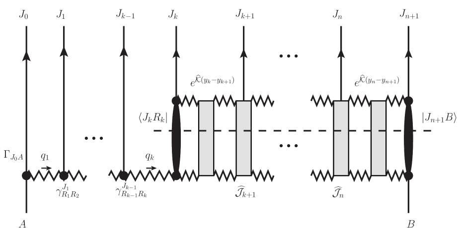
Figure 2: Schematic representation of the discontinuity of ${\cal A}^{\{-\}}_{2\rightarrow n+2}$ in $s_{k,n+1}$-channel

The zig-zag lines represent Reggeized gluon exchange. The dashed line denotes on-mass-shell states in the unitarity condition. The right and the left black ovals represent the impact-factors for particle-jet and Reggeon-jet transitions respectively. The right-angled grey blocks denote the operators of the jet production. The blank right-angled block in the $t_{k+1}$-channel represents the operator $e^{\hat{\cal K}(y_{k}-y_{k+1})}$.

$$\begin{split}&-4i(2\pi)^{D-2}\delta^{\bot}(q_{k}-q_{n+1}-\sum_{l=k}^{n}k_{l})\mathrm{disc}_{s_{k,n+1}}{\cal A}_{2\rightarrow 2+n}^{\{-\}}=\\ &=2s\Gamma_{J_{0}A}^{R_{1}}\frac{e^{\omega(q_{1})(y_{0}-y_{1})}}{q_{1\bot}^{2}}\Biggl{(}\prod_{l=2}^{k}\gamma_{R_{l-1}R_{l}}^{J_{l-1}}\frac{e^{\omega(q_{l})(y_{l-1}-y_{l})}}{q_{l\bot}^{2}}\Biggr{)}\langle J_{k}R_{k}|\Biggl{(}\prod_{l=k+1}^{n}e^{\widehat{\cal K}(y_{l-1}-y_{l})}\widehat{\cal J}_{l}\Biggr{)}e^{\widehat{\cal K}(y_{n}-y_{n+1})}|J_{n+1}B\rangle.\end{split}$$

Here the ket-states $|J_{n+1}B\rangle$ and the bra-states $\langle J_{k}R_{k}|$ denote the impact factors for the particle-jet $B\rightarrow J_{n+1}$ and the Reggeon-jet $R_{k}\rightarrow J_{k}$ transitions respectively, $\widehat{\cal K}$ and $\widehat{\cal J}_{l}$ are the operators of the BFKL kernel and the jet production. The states are defined by their projections on the two-Reggeon states with the normalization (4.4) and the operators are specified by their matrix elements.

The discontinuity in any $s_{i,j}$ - channel $(i<j)$ can be obtained from (4.1) by an appropriate substitution. If $i=0$, $k$ must be changed on $i$, all factors besides $2s$ on the left from $\langle J_{k}R_{k}|$ must be omitted and $\langle J_{k}R_{k}|$ must be replaced by $\langle J_{0}A|$; if $j<n+1$, $n$ must be changed on $j-1$ and $|J_{n+1}B\rangle$ must be replaced by $\frac{e^{\omega(q_{j+1})(y_{j}-y_{j+1})}}{q_{(j+1)\bot}^{2}}\Biggl{(}\prod_{m=j+2}^{n+1}\gamma_{R_{m-1}R_{m}}^{J_{m-1}}\frac{e^{\omega(q_{m})(y_{m-1}-y_{m})}}{q_{m\bot}^{2}}\Biggr{)}\Gamma_{J_{n+1}B}^{R_{n+1}}$.

The BFKL kernel consists of two parts,

$$\hat{\cal K}=\omega(\hat{r}_{1})+\omega(\hat{r}_{2})+\hat{\cal K}_{r},$$ (4.5)

where the ‘‘virtual’’ part is given by the gluon trajectories and the ‘‘real’’ part ${\cal K}_{r}$ appears from real particle production. In the NLO

$$\hat{\cal K}_{r}\ =\ \hat{\cal K}^{\Delta}_{r}-\hat{\cal K}^{B}_{r}\hat{\cal K}^{B}_{r}\Delta\,,$$ (4.6)

where $\Delta\gg 1$ is an auxiliary parameter serving for separation of QMRK from pure MRK, ${\cal K}^{B}_{r}$ is the LO (Born) real kernel and

$$\langle{\cal G}_{1}{\cal G}_{2}|\hat{\cal K}^{\Delta}_{r}|{\cal G}^{\prime}_{1}{\cal G}^{\prime}_{2}\rangle=\delta^{\bot}(r_{1}+r_{2}-r^{\prime}_{1}-r^{\prime}_{2})\sum_{J}\!\int\!\!\gamma^{J}_{{\cal G}_{1}{\cal G}^{\prime}_{1}}\gamma_{J}^{{\cal G}_{2}{\cal G}^{\prime}_{2}}\frac{d\phi_{J}}{2(2\pi)^{D-1}}\theta(\Delta-\Delta_{J}).$$ (4.7)

Here the sum is taken over all possible jets and over all discrete quantum numbers of these jets, $\gamma_{J}^{{\cal G}_{2}{\cal G}^{\prime}_{2}}$ is the effective vertex for absorption of the jet $J$ in the Reggeon transition ${\cal G}^{\prime}_{2}\rightarrow{\cal G}_{2}$ which is related to $\gamma^{\bar{J}}_{{\cal G}_{2}{\cal G}^{\prime}_{2}}$ by the change of signs of longitudinal momenta and the corresponding change of wave functions;

$$d\phi_{J}=(2\pi)^{D}\delta^{D}\Bigl{(}l_{J}-\sum_{i}l_{i}\Bigr{)}\frac{1}{n!}\frac{dl^{2}_{J}}{2\pi}\prod_{i}\frac{d^{D-1}l_{i}}{2l^{0}_{i}(2\pi)^{D-1}}~{},$$ (4.8)

where $l_{i}$ are the jet particle momenta, $n$ is a number of identical particles in the jet; $\Delta_{J}$ in (4.7) is the interval between the rapidities $z_{i}=\frac{1}{2}\ln[{l^{+}_{i}}/{l^{-}_{i}}]$ of the jet particles. In the Born kernel the second term in (4.6) is omitted and only one-gluon production in the LO is accounted in (4.7).

Formally the representation of the kernel by Eqs. (4.5)–(4.8) remains the same as in QCD. The difference is in appearance of new Reggeon vertices in the sum over $J$ in (4.7) and in the changes of the gluon trajectory and of the QCD Reggeon vertices because of dependence of the fermion contributions on representation of the colour group and appearance of scalar contributions. The same applies to the representations of the impact factors and the operator of the jet production. Remind that they have to be taken in the NLO in the case of one-particle jets and in the LO in the case of two-particle jets. The particle-particle impact-factor for the $B\rightarrow B^{\prime}$ ($B$ and $B^{\prime}$ can be two-particle jets as well) transition is represented by the ket-state $|\bar{B}^{\prime}B\rangle$ defined as

$$|\bar{B}^{\prime}B\rangle\ =\ |\bar{B}^{\prime}B\rangle^{\Delta}-\left({\omega(\hat{r}_{1\bot}^{2})}\ln\left|\frac{\hat{r}_{1\bot}}{q_{B\bot}}\right|+{\omega(\hat{r}_{2\bot}^{2})}\ln\left|\frac{\hat{r}_{2\bot}}{q_{B\bot}}\right|+\hat{\cal K}^{B}_{r}\;\Delta\right)|\bar{B}^{\prime}B\rangle^{B},$$ (4.9)

where $|\bar{B}^{\prime}B\rangle^{B}$ is the LO (Born) impact factor and

$$\langle{\cal G}_{1}{\cal G}_{2}|\bar{B}^{\prime}B\rangle^{\Delta}=\delta^{\bot}(q_{B}-r_{1}-r_{2})\sum_{J}\!\int\!\!\left(\Gamma^{{\cal G}_{1}}_{JB}\Gamma^{{\cal G}_{2}}_{B^{\prime}J}-\Gamma^{{\cal G}_{2}}_{JB}\Gamma^{{\cal G}_{1}}_{B^{\prime}J}\right)d\phi_{J}\prod_{l}\theta\Big{(}\Delta-(z_{l}-y_{B})\Big{)}\,.$$ (4.10)

Here $q_{B}=p_{B^{\prime}}-p_{B}$, $z_{l}$ are the rapidities of particles in the intermediate jets and $y_{B}=\ln|q_{B\bot}|/(\sqrt{2}p_{B}^{-})$. case when $B$ or $B^{\prime}$ is a two-particle jet, only the first term must be kept in Eq. (4.9); moreover, only the Born approximation for this term must be taken in Eq. (4.10).

For completeness let us present the impact-factor of the $A\rightarrow A^{\prime}$ transition, although it is not necessary since it can obtained from (4.9), (4.10) by the ‘‘left $\leftrightarrow$ right’’ exchange, which means $|\;\rangle\leftrightarrow\langle\;|,\;A\leftrightarrow B,\;\vec{r}_{i}\leftrightarrow-\vec{r}_{i},\;z_{l}\leftrightarrow-z_{l}\;y_{A}\leftrightarrow-y_{B},\;\vec{q}_{i}\leftrightarrow-\vec{q}_{i},+\leftrightarrow-$.

$$\langle A^{\prime}\bar{A}|\ =\ \langle A^{\prime}\bar{A}|^{\Delta}-\langle A^{\prime}\bar{A}|^{B}\left({\omega(\hat{r}_{1\bot}^{2})}\ln\left|\frac{\hat{r}_{1\bot}}{q_{A\bot}}\right|+{\omega^{B}(\hat{r}_{2})}\ln\left|\frac{\hat{r}_{2\bot}^{2}}{q_{A\bot}}\right|+\hat{\cal K}_{r}^{B}\;\Delta\right),$$ (4.11)

$$\langle A^{\prime}\bar{A}|{\cal G}_{1}{\cal G}_{2}\rangle^{\Delta}=\delta^{\bot}(q_{A}-r_{1}-r_{2})\sum_{\tilde{A}}\!\int\!\!\left(\Gamma^{{\cal G}_{1}}_{\tilde{A}A}\Gamma^{{\cal G}_{2}}_{A^{\prime}\tilde{A}}-\Gamma^{{\cal G}_{2}}_{\tilde{A}A}\Gamma^{{\cal G}_{1}}_{A^{\prime}\tilde{A}}\right)d\phi_{\tilde{A}}\prod_{l}\theta\Big{(}\Delta-(y_{A}-z_{l})\Big{)},$$ (4.12)

where $q_{A}=p_{A}-p_{A^{\prime}}$, $y_{A}=\ln(\sqrt{2}p_{A}^{+}/|q_{A\bot}|)$.

Accordingly, the Reggeon-particle impact factors are defined as

$$|\bar{J}_{i}R_{i+1}\rangle\ =\ |\bar{J}_{i}R_{i+1}\rangle^{\Delta}-\left(\frac{\omega(q_{(i+1)\bot}^{2})}{2}\ln\left|\frac{k^{2}_{i\bot}}{|q_{(i+1)\bot}-\hat{r}_{1\bot}||q_{(i+1)\bot}-\hat{r}_{2\bot}|}\right|\right.$$

$$\left.-\frac{\omega(\hat{r}_{1\bot}^{2})}{2}\ln\left|\frac{k^{2}_{i\bot}}{|q_{(i+1)\bot}-\hat{r}_{1\bot}|\hat{r}_{1\bot}}\right|-\frac{\omega(\hat{r}_{2\bot}^{2})}{2}\ln\left|\frac{k^{2}_{i\bot}}{|q_{(i+1)\bot}-\hat{r}_{2\bot}|\hat{r}_{2\bot}}\right|+\hat{\cal K}_{r}^{B}\Delta\right)|\bar{J}_{i}R_{i+1}\rangle^{B}\,,$$ (4.13)

$$\langle{\cal G}_{1}{\cal G}_{2}|\bar{J}_{i}R_{i+1}\rangle^{\Delta}\ =\ \delta^{\bot}(q_{(i+1)}+k_{i}-r_{1}-r_{2})\times$$

$$\times\ \sum_{J}\int\left(\gamma^{J}_{{\cal G}_{1}R_{i+1}}\Gamma^{{\cal G}_{2}}_{J_{i}J}-\gamma^{J}_{{\cal G}_{2}R_{i+1}}\Gamma^{{\cal G}_{1}}_{J_{i}J}\right)d\phi_{J}\prod_{l}\theta\Big{(}\Delta-(z_{l}-y_{i})\Big{)},$$ (4.14)

and

$$\langle J_{i}R_{i}|\ =\ \langle J_{i}R_{i}|^{\Delta}-\langle J_{i}R_{i}|^{B}\left(\frac{\omega(q_{i\bot}^{2})}{2}\ln\left|\frac{k^{2}_{i\bot}}{|q_{i\bot}-\hat{r}_{1\bot}||q_{i\bot}-\hat{r}_{2\bot}|}\right|\right.$$

$$\left.-\frac{\omega(\hat{r}_{1\bot}^{2})}{2}\ln\left|\frac{k^{2}_{i\bot}}{|q_{i\bot}-\hat{r}_{1\bot}|\hat{r}_{1\bot}}\right|-\frac{\omega(\hat{r}_{2\bot}^{2})}{2}\ln\left|\frac{k^{2}_{i\bot}}{|q_{i\bot}-\hat{r}_{2\bot}|\hat{r}_{2\bot}}\right|+\hat{\cal K}_{r}^{B}\Delta\right),$$ (4.15)

$$\langle J_{i}R_{i}|{\cal G}_{1}{\cal G}_{2}\rangle^{\Delta}\ =\ \delta^{\bot}(r_{1}+r_{2}-q_{i}+k_{i})\times$$

$$\times\ \sum_{J}\int\left(\gamma^{J}_{R_{i}{\cal G}_{1}}\Gamma^{{\cal G}_{2}}_{J_{i}J}-\gamma^{J}_{R_{i}{\cal G}_{2}}\Gamma^{{\cal G}_{1}}_{J_{i}J}\right)d\phi_{J}\prod_{l}\theta\Big{(}\Delta-(y_{i}-z_{l})\Big{)}.$$ (4.16)

And finally, the operators ${\hat{\cal J}}_{i}$ for production of jets $J_{i}$ are defined as

$$\hat{\cal J}_{i}=\hat{\cal J}_{i}^{\Delta}-\left(\hat{\cal K}^{B}_{r}\hat{\cal J}^{B}_{i}+\hat{\cal J}^{B}_{i}\hat{\cal K}^{B}_{r}\right)\Delta,\quad\langle{\cal G}_{1}{\cal G}_{2}|\hat{\cal\cal J}^{\Delta}_{i}|{\cal G}^{\prime}_{1}{\cal G}^{\prime}_{2}\rangle=\delta^{\bot}(r_{1}+r_{2}-k_{i}-r^{\prime}_{1}-r^{\prime}_{2})\times$$

$$\times\quad\Bigg{[}\gamma^{J_{i}}_{{\cal G}_{1}{\cal G}^{\prime}_{1}}\delta^{\bot}(r_{2}-r^{\prime}_{2})r_{2\perp}^{~{}2}\delta_{{\cal G}_{2}{\cal G}_{2}^{\prime}}+\gamma^{J_{i}}_{{\cal G}_{2}{\cal G}^{\prime}_{2}}\delta^{\bot}(r_{1}-r^{\prime}_{1})r_{1\perp}^{~{}2}\delta_{{\cal G}_{1}{\cal G}_{1}^{\prime}}+$$

$$+\quad\sum_{G}\int_{y_{i}-\Delta}^{y_{i}+\Delta}\frac{dz_{G}}{2(2\pi)^{D-1}}\left(\gamma^{\{J_{i}G\}}_{{\cal G}_{1}{\cal G}^{\prime}_{1}}\gamma^{{\cal G}_{2}{\cal G}^{\prime}_{2}}_{G}+\gamma^{G}_{{\cal G}_{1}{\cal G}^{\prime}_{1}}\gamma^{{\cal G}_{2}{\cal G}^{\prime}_{2}}_{J_{i}G}\right)\Bigg{]}.$$ (4.17)

Here the last term appears only in the case when $J_{i}\equiv G_{i}$ is a single gluon, the sum in this term goes over quantum numbers of the intermediate gluon $G$ and the vertices must be taken in the Born approximation. At that $\gamma^{\{J_{i}G\}}_{{\cal G}_{1}{\cal G}^{\prime}_{1}}$ is the vertex for production of the jet consisting of the gluons $G_{i}$ and $G$, $\;\;\gamma^{{\cal G}_{2}{\cal G}^{\prime}_{2}}_{G_{i}G}$ is the vertex for absorption of gluon $G$ and production of gluon $G_{i}$ in the ${\cal G}_{2}\to{\cal G}^{\prime}_{2}$ transition; it can be obtained from $\gamma_{{\cal G}_{2}{\cal G}^{\prime}_{2}}^{\{G_{i}G\}}$ by crossing with respect to the gluon $G$.

4.2 Bootstrap conditions

In QCD, it was proved in [29] that an infinite number of the bootstrap relations (4.3) providing the validity of the multi-Regge form (2.1) in the NLLA is fulfilled if several bootstrap conditions are performed. This statement remains correct for Yang-Mills theories containing fermions and scalars in arbitrary representations of the colour group with any Yukawa-type interaction, because formally all components of the discontinuities entering in the bootstrap relations (4.3) differ from corresponding components in QCD only by appearance of new Reggeon vertices and by the changes of the gluon trajectory and of the QCD Reggeon vertices due to dependence of the fermion contributions on representation of the colour group and emergence of scalar contributions. Moreover, the bootstrap conditions have the same form as in QCD. They ere the following.

The particle-jet impact factors are proportional to their Reggeon vertices:

$$\langle{A^{\prime}A}|={g}\langle R_{\omega}(q_{A})|\Gamma^{R}_{A^{\prime}A}~{},\;\;|{B^{\prime}B}\rangle={g}\Gamma^{R}_{B^{\prime}B}|R_{\omega}(q_{B})\rangle~{},\;\;$$ (4.18)

where $\Gamma^{R}_{A^{\prime}A}$ and $\Gamma^{R}_{B^{\prime}B}$ are the Reggeon vertices, $q_{A}=p_{A}-p_{A^{\prime}},\;\;q_{B}=p_{B^{\prime}}-p_{B},\;\;$ and $|R_{\omega}(q)\rangle$ are the universal (process independent) states.

The states $|R_{\omega}(q)\rangle$ are the eigenstate of the kernel $\hat{\cal K}$ with the eigenvalues $\omega(q)$

$$(\hat{\cal K}-\omega(q))|R_{\omega}(q)\rangle=0,\;\;\langle R_{\omega}(q)|(\hat{\cal K}-\omega(q))=0.$$ (4.19)

Moreover, they satisfy the orthonormality relations

$$\frac{g^{2}t}{2(2\pi)^{D-1}}\langle R^{\prime}_{\omega}(q^{\prime})|R_{\omega}(q)\rangle=-\omega(t)\delta^{\bot}(q-q^{\prime})\delta^{RR^{\prime}}~{}.$$ (4.20)

The Reggeon-particle impact factors and the jet production vertices satisfy the conditions

$$gq_{i\perp}^{2}\langle R_{\omega}(q_{i})|{\hat{\cal J}_{i}}+\langle{{\cal J}_{i}}R_{i}|={g}\gamma^{{\cal J}_{i}}_{R_{i}R_{i+1}}\langle R_{\omega}(q_{i+1})|,$$

$$gq^{2}_{(i+1)\perp}{\hat{\cal J}_{i}}|R_{\omega}(q_{i+1})\rangle+|{\cal J}_{i}R_{i+1}\rangle={g}\gamma^{{\cal J}_{i}}_{R_{i}R_{i+1}}|R_{\omega}(q_{i})\rangle~{}.$$ (4.21)

The summation over Reggeon colour index $R$ in the right-hand sides of Eqs. (4.18) and (4.21) is assumed.

5 Proof of fulfilment of the bootstrap conditions

In QCD, the bootstrap conditions (4.18)-(4.20) were formulated in [61, 62, 63, 64, 65, 67] and their fulfilment was proved in [68, 62, 51, 49, 64, 69, 65, 66, 70, 56]. The bootstrap conditions (4.21) were derived in [67] and their fulfilment was proved in [71, 72, 73].

To extend the proof to Yang-Mills theories of general form one has to take three steps. First, one needs to generalize the proof of the QCD bootstrap conditions to the case of fermions in arbitrary representation of the colour group. Second, one has to prove that contributions of scalars in these conditions don’t violate their fulfilment. And third, one has to prove fulfilment of new bootstrap conditions.

5.1 Impact-factors for particle-jet transitions

We have to separate consideration of one-particle and two-particle jets. Corresponding impact factors we will call particle $\rightarrow$ particle and particle $\rightarrow$ jet ones. In the NLLA the first ones must be taken in the NLO, while for the second ones the Born approximation is sufficient. Let us start with particle-particle impact factors.

5.1.1 Particle $\rightarrow$ particle impact-factors

In QCD they are the gluon and quark ones. The first of them was obtained in [51]. The derivation presented there permits to generalize the quark contribution to this impact factor to any representation of the colour group. Using also the results of [42] for the scalar contribution, we obtain

$$\langle G^{\prime}G|{\cal G}_{1}{\cal G}_{2}\rangle=\delta^{\bot}(q-r_{1}-r_{2})g^{2}e(p_{G})_{\perp\mu}e(p_{G^{\prime}})^{*}_{\perp\nu}T^{R}_{G^{\prime}G}T^{R}_{{\cal G}_{1}{\cal G}_{2}}\Biggl{\{}-g_{\bot}^{\mu\nu}\Biggl{[}1-\bar{g}^{2}\frac{\Gamma^{2}(1+\epsilon)}{\epsilon\Gamma(1+2\epsilon)}(-q_{\bot}^{2})^{\epsilon}\biggl{[}{\tilde{K}_{1}}$$

$$+\left(\left(\frac{r_{1\bot}^{\>2}}{q_{\bot}^{\>2}}\right)^{\epsilon}+\left(\frac{r_{2\bot}^{\>2}}{q_{\bot}^{\>2}}\right)^{\epsilon}-1\right)\biggl{(}\frac{1}{2\epsilon}+\psi(1+2\epsilon)-\psi(1+\epsilon)+\frac{a_{1}}{2(1+2\epsilon)(3+2\epsilon)}\biggr{)}$$

$$+\frac{3}{2\epsilon}+2\psi(1)-\psi(1+\epsilon)-\psi(1+2\epsilon)-\frac{(1+\epsilon)^{2}\;a_{1}+2\epsilon^{2}a_{2}}{2(1+\epsilon)^{2}(1+2\epsilon)(3+2\epsilon)}\biggr{]}$$

$$-\left(g^{\mu\nu}_{\perp}-(D-2)\frac{q^{\mu}_{\perp}q^{\nu}_{\perp}}{q^{2}_{\perp}}\right)\bar{g}^{2}\frac{\Gamma^{2}(1+\epsilon)}{\Gamma(4+2\epsilon)}(-q_{\bot}^{2})^{\epsilon}\;\frac{2a_{2}}{(1+\epsilon)}\biggr{\}},$$ (5.1)

where $q=r_{1}+r_{2}$ and

$${\tilde{K}_{1}}=-\frac{(4\pi)^{2+\epsilon}\Gamma(1+2\epsilon)\epsilon\left(-q_{\bot}^{\>2}\right)^{-\epsilon}}{4\Gamma(1-\epsilon)\Gamma^{2}(1+\epsilon)}\int\frac{d^{D-2}l}{(2\pi)^{D-1}}\ln\left(\frac{q_{\bot}^{\>2}}{l_{\bot}^{2}}\right)\frac{q_{\bot}^{\>2}}{(l-r_{1})_{\bot}^{2}(l+r_{2})_{\bot}^{2}}$$

$$=\frac{1}{2\epsilon}\left(2-\left(\frac{r_{1\bot}^{\>2}}{q_{\bot}^{\>2}}\right)^{\epsilon}-\left(\frac{r_{2\bot}^{\>2}}{q_{\bot}^{\>2}}\right)^{\epsilon}\right)+\frac{\epsilon}{2}\ln\left(\frac{r_{1\bot}^{\>2}}{q_{\bot}^{\>2}}\right)\ln\left(\frac{r_{2\bot}^{\>2}}{q_{\bot}^{\>2}}\right)-4\epsilon^{2}\zeta(3)+{\cal O}(\epsilon^{3})\;.$$ (5.2)

Remind that

$$a_{1}=11+7\epsilon-4(1+\epsilon)\xi_{f}-{\xi_{s}},\;\;a_{2}=1+\epsilon-2\xi_{f}+{\xi_{s}}~{}$$ (5.3)

and the coefficients $a_{1}$ and $a_{2}$ vanish in $N=4$ SYM in the dimensional reduction.

Comparing (5.1) with gluon-gluon-Reggeon vertex (3.10) we see that the bootstrap relation (4.18) is fulfilled if

$$\langle R_{\omega}(q)|{\cal G}_{1}{\cal G}_{2}\rangle=\delta^{\bot}(q-r_{1}-r_{2})T^{R}_{{\cal G}_{1}{\cal G}_{2}}\biggl{(}1-\bar{g}^{2}\frac{\Gamma^{2}(1+\epsilon)}{\epsilon\Gamma(1+2\epsilon)}(-q_{\bot}^{2})^{\epsilon}\biggl{[}{\tilde{K}_{1}}+\left(\left(\frac{r_{1\bot}^{\>2}}{q_{\bot}^{\>2}}\right)^{\epsilon}+\left(\frac{r_{2\bot}^{\>2}}{q_{\bot}^{\>2}}\right)^{\epsilon}-1\right)$$

$$\times\biggl{\{}\frac{1}{2\epsilon}+\psi(1+2\epsilon)-\psi(1+\epsilon)+\frac{a_{1}}{2(1+2\epsilon)(3+2\epsilon)}\biggr{\}}$$

$$-\frac{1}{2\epsilon}+\psi(1)+\psi(1+\epsilon)-\psi(1-\epsilon)-\psi(1+2\epsilon)\biggr{]}\biggr{)}\;.$$ (5.4)

The quark impact factor in QCD was obtained in [49]. The calculations presented there can be easily generalized to any quark representation of the colour group. Scalars give contributions to the quark impact factors due to their gauge and Yukawa-type interactions. The first ones come from vacuum polarization diagrams only and are obtained from corresponding quark contributions by the replacement $\xi_{f}\rightarrow\xi_{s}/(4(1+\epsilon))$. As for the second ones, fulfilment of the bootstrap conditions (4.18) for them was proved recently [42] in the general form, for all impact factors, using the analytic properties of the amplitudes whose imaginary parts are associated with the impact factors and the vertices in the bootstrap conditions (4.18). Using these results, we obtain

$$\langle Q^{\prime}_{f}Q_{i}|{\cal G}_{1}{\cal G}_{2}\rangle=\delta^{\bot}(q-r_{1}-r_{2})\delta_{fi}g^{2}\bar{u}_{f}(p^{\prime})t^{R}_{i}\frac{n\mspace{-8.0mu}/_{2}}{2p^{+}}u_{i}(p)\;T^{R}_{{\cal G}_{1}{\cal G}_{2}}\Biggl{[}1-\bar{g}^{2}\frac{\Gamma^{2}(1+\epsilon)}{\epsilon\Gamma(1+2\epsilon)}(-q_{\bot}^{2})^{\epsilon}\biggl{[}{\tilde{K}_{1}}$$

$$+\left(\left(\frac{r_{1\bot}^{\>2}}{q_{\bot}^{\>2}}\right)^{\epsilon}+\left(\frac{r_{2\bot}^{\>2}}{q_{\bot}^{\>2}}\right)^{\epsilon}-1\right)\biggl{(}\frac{1}{2\epsilon}+\psi(1+2\epsilon)-\psi(1+\epsilon)+\frac{a_{1}}{2(1+2\epsilon)(3+2\epsilon)}\biggr{)}$$

$$+\frac{1}{2\epsilon}+2\psi(1)-\psi(1+\epsilon)-\psi(1+2\epsilon)+\frac{a_{1}-3(3+2\epsilon)}{2(1+2\epsilon)(3+2\epsilon)}+\left(\frac{2C_{F}^{i}}{N_{c}}-1\right)\left(\frac{1}{\epsilon}-\frac{3-2\epsilon}{2(1+2\epsilon)}\right)\biggr{]}\Biggr{]}$$

$$+\delta^{\bot}(q-r_{1}-r_{2})\Gamma_{Q^{\prime}_{f}Q_{i}}^{R(Y)}\;gT^{R}_{{\cal G}_{1}{\cal G}_{2}}\;.$$ (5.5)

Fulfilment of the bootstrap condition (4.18) for the quark impact factor follows from comparison of this result with (3.12) and (5.4).

To obtain the impact factors for scalar particles we use the results of [42]. In this paper they were calculated in SYM and in the special scheme which simplifies check of the bootstrap conditions (we call it bootstrap scheme). Generalization of the results of [42] to any representations of the colour group for quarks and scalars is carried out in the same way as for the quark impact factors. Going well to the standard scheme with the help of the equality

$$\langle R^{B}_{\omega}(q)|\widehat{\cal U}_{q}|{\cal G}_{1}{\cal G}_{2}\rangle=\delta^{\bot}(q-r_{1}-r_{2})T^{R}_{{\cal G}_{1}{\cal G}_{2}}\bar{g}^{2}\frac{\Gamma^{2}(1+\epsilon)}{\epsilon\Gamma(1+2\epsilon)}(-q_{\bot}^{2})^{\epsilon}$$

$$\times\biggl{[}-{\tilde{K}_{1}}+\left(\left(\frac{r_{1\bot}^{\>2}}{q_{\bot}^{\>2}}\right)^{\epsilon}+\left(\frac{r_{2\bot}^{\>2}}{q_{\bot}^{\>2}}\right)^{\epsilon}\right)\biggl{(}\frac{1}{2\epsilon}-\psi(1)-\psi(1+\epsilon)+\psi(1-\epsilon)+\psi(1+2\epsilon)\biggr{)}$$

$$-\left(\frac{r_{1\bot}^{\>2}}{q_{\bot}^{\>2}}\right)^{\epsilon}\ln\left(\frac{r_{1\bot}^{\>2}}{q_{\bot}^{\>2}}\right)-\left(\frac{r_{2\bot}^{\>2}}{q_{\bot}^{\>2}}\right)^{\epsilon}\ln\left(\frac{r_{2\bot}^{\>2}}{q_{\bot}^{\>2}}\right)\biggr{]},$$ (5.6)

where

$$\begin{split}&\langle{\cal G}_{1}^{\prime}{\cal G}_{2}^{\prime}|\widehat{\cal U}_{K}|{\cal G}_{1}{\cal G}_{2}\rangle=g^{2}\delta^{\bot}(r_{1}^{\prime}+r_{2}^{\prime}-r_{1}-r_{2})T^{a}_{{\cal G}_{1}^{\prime}{\cal G}_{1}}T^{a}_{{\cal G}_{2}{\cal G}_{2}^{\prime}}\frac{r_{1\bot}^{{}^{\prime}2}r_{2\bot}^{{}^{\prime}2}}{(2\pi)^{D-1}}\biggl{(}\frac{r_{1\bot}^{{}^{\prime}\alpha}}{r_{1\bot}^{{}^{\prime}2}}+\frac{(r_{1}-r_{1}^{\prime})_{\bot}^{\alpha}}{(r_{1}-r_{1}^{\prime})_{\bot}^{2}}\biggr{)}\times\\ &\times\biggl{(}\frac{r_{2\bot\alpha}^{{}^{\prime}}}{r_{2\bot}^{{}^{\prime}2}}+\frac{(r_{2}-r_{2}^{\prime})_{\bot\alpha}}{(r_{2}-r_{2}^{\prime})_{\bot}^{2}}\biggr{)}\ln\Big{[}\frac{K_{\bot}^{2}}{(r_{1}^{\prime}-r_{1})_{\bot}^{2}}\Big{]}=\frac{1}{2}\ln\Bigl{[}\frac{K_{\bot}^{2}}{(r_{1}-r_{1}^{\prime})_{\bot}^{2}}\Bigr{]}\langle{\cal G}_{1}^{\prime}{\cal G}_{2}^{\prime}|\widehat{\cal K}_{r}^{B}|{\cal G}_{1}{\cal G}_{2}\rangle\end{split}$$ (5.7)

and ${\tilde{K}_{1}}$ is defined in (5.2), we obtain

$$\langle S^{\prime}_{r^{\prime}}S_{r}|{\cal G}_{1}{\cal G}_{2}\rangle=\delta^{\bot}(q-r_{1}-r_{2})\delta_{r^{\prime}r}g^{2}({\cal T}_{r}^{R})_{S^{\prime}_{r^{\prime}}S_{r}}\;T^{R}_{{\cal G}_{1}{\cal G}_{2}}\Biggl{[}1-\bar{g}^{2}\frac{\Gamma^{2}(1+\epsilon)}{\epsilon\Gamma(1+2\epsilon)}(-q_{\bot}^{2})^{\epsilon}\biggl{[}{\tilde{K}_{1}}$$

$$+\left(\left(\frac{r_{1\bot}^{\>2}}{q_{\bot}^{\>2}}\right)^{\epsilon}+\left(\frac{r_{2\bot}^{\>2}}{q_{\bot}^{\>2}}\right)^{\epsilon}\right)\biggl{(}\frac{1}{2\epsilon}+\psi(1+2\epsilon)-\psi(1+\epsilon)+\frac{a_{1}}{2(1+2\epsilon)(3+2\epsilon)}\biggr{)}$$

$$+2\psi(1)-2\psi(2+2\epsilon)+\left(\frac{2C^{r}_{S}}{N_{c}}\right)\left(\frac{1}{\epsilon}-\frac{2}{(1+2\epsilon)}\right)\biggr{]}$$

$$+\delta^{\bot}(q-r_{1}-r_{2})\Gamma_{S^{\prime}_{r^{\prime}}S_{r}}^{R(Y)}\;gT^{R}_{{\cal G}_{1}{\cal G}_{2}}\;.$$ (5.8)

Fulfilment of the bootstrap condition (4.18) for scalar scattering follows from comparison of this result with (LABEL:eq:SRSc) and (5.4).

5.1.2 particle $\rightarrow$ jet impact factors

For particle $\rightarrow$ jet transitions $A\rightarrow A^{\prime}=\{P_{1}P_{2}\}$ the bootstrap condition (4.18) takes the form

$$\langle\{P_{1}P_{2}\}A|{\cal G}_{1}{\cal G}_{2}\rangle=g\Gamma_{\{P_{1}P_{2}\}A}^{R}\langle R_{\omega}(q)|{\cal G}_{1}{\cal G}_{2}\rangle\,,$$ (5.9)

where

$$\langle\{P_{1}P_{2}\}A|{\cal G}_{1}{\cal G}_{2}\rangle=\delta^{\bot}(k-k_{1}-k_{2}-r_{1}-r_{2})\Bigl{(}\sum_{\{A^{\prime}\}}\Gamma_{\{P_{1}P_{2}\}A^{\prime}}^{{\cal G}_{2}}\Gamma_{A^{\prime}A}^{{\cal G}_{1}}+$$ (5.10)

$$+\sum_{\{P_{1}^{\prime}\}}\Gamma_{P_{1}P^{\prime}_{1}}^{{\cal G}_{2}}\Gamma_{\{P^{\prime}_{1}P_{2}\}A}^{{\cal G}_{1}}+\sum_{\{P^{\prime}_{2}\}}\Gamma_{P_{2}P^{\prime}_{2}}^{{\cal G}_{2}}\Gamma_{\{P_{1}P^{\prime}_{2}\}A}^{{\cal G}_{1}}\Bigr{)}-\{{\cal G}_{1}\leftrightarrow{\cal G}_{2}\}\,.$$

As it was already pointed out we need to consider Eqs. (5.9) and (5.10) in the LO only. In this approximation fulfilment of the bootstrap conditions (5.9) can be proved without explicit forms of the impact factors [42]. Indeed, using the old-fashioned perturbation theory we can write

$$\Gamma_{\{CD\}B}^{R}=\sum_{B^{\prime}}\frac{V_{\{CD\}B^{\prime}}\Gamma_{B^{\prime}B}^{R}}{2\epsilon_{B^{\prime}}(\epsilon_{C}+\epsilon_{D}-\epsilon_{B^{\prime}})}+\sum_{C^{\prime}}\frac{\Gamma_{CC^{\prime}}^{R}V_{\{C^{\prime}D\}B}}{2\epsilon_{B}(\epsilon_{B}-\epsilon_{D}-\epsilon_{C^{\prime}})}+\sum_{D^{\prime}}\frac{\Gamma_{DD^{\prime}}^{R}V_{\{CD^{\prime}\}B}}{2\epsilon_{B}(\epsilon_{B}-\epsilon_{D^{\prime}}-\epsilon_{C})}\,,$$ (5.11)

where $V_{\{BC\}A}$ is the vertex of the $A\rightarrow BC$ transition in which all particle momenta are on the mass shell and all particle polarizations are physical. It is easy to see that in the impact factor (5.10) the contributions resulting from use for $\Gamma_{\{P_{1}P_{2}\}A^{\prime}}^{{\cal G}_{2}}$ the last two terms in the representation (5.11) cancel the contributions resulting from use for $\Gamma_{\{P^{\prime}_{1}P_{2}\}A}^{{\cal G}_{1}}$ and $\Gamma_{\{P_{1}P^{\prime}_{2}\}A}^{{\cal G}_{1}}$ the first term in (5.11). Further, the sum of the contributions coming from use for $\Gamma_{\{P^{\prime}_{1}P_{2}\}A}^{{\cal G}_{1}}$ the third term in (5.11) and for $\Gamma_{\{P_{1}P^{\prime}_{2}\}A}^{{\cal G}_{1}}$ the second term cancel each other with account of the antisymmetrization $\{{\cal G}_{1}\leftrightarrow{\cal G}_{2}\}$. After these cancellation, it’s easy to see that fulfilment of (5.9) follows from the relation

$$\sum_{B}\Gamma_{BA}^{{\cal G}_{1}}\Gamma_{CB}^{{\cal G}_{2}}-\{{\cal G}_{1}\leftrightarrow{\cal G}_{2}\}=gT^{R}_{{\cal G}_{1}{\cal G}_{2}}\Gamma_{CA}^{R}\,,$$ (5.12)

which is the LO bootstrap condition for the particle-particle impact factors.

5.2 Bootstrap conditions for the eigenfunction of the BFKL kernel

Fulfilment of the bootstrap conditions (4.19) and (4.20) were proved in QCD in [68, 62, 63, 69, 70]. In fact, the proof can be applied to Yang-Mills theories with quarks and scalars in any representations of the colour group and with any Yukawa-type interactions. First, the kernel $\hat{\cal K}$, the eigenstate $|R_{\omega}(q)\rangle$ and the eigenvalue $\omega(q)$ don’t depend on the Yukawa-type interactions at all. For the kernel it follows from its definition (4.5) – (4.7) and from the explicit form of the Reggeon production vertices presented in Sections 3.2 and 3.3; for the trajectory and for the eigenstate $|R_{\omega}\rangle$ it is seen from their explicit forms presented in (3.1) – (3.3) and (5.4). Second, it’s seen also from these equations that the quark contributions to the trajectory and to the eigenfunction depend on the quark representation only through $\xi_{f}$ and the scalar contributions is obtained from the quark one by the replacement $\xi_{f}\rightarrow\xi_{s}/(4(1+\epsilon))$. The same is true for the BFKL kernel in the antisymmetric adjoint representation of the colour group [31, 74] which enters into the bootstrap condition (4.19). Therefore generalization of the proof of fulfilment of the bootstrap conditions (4.19) and (4.20) presented to Yang-Mills theories with quarks and scalars in any representations of the colour group is trivial.

5.3 Bootstrap conditions for particle production in the central rapidity region

In the NLLA, the bootstrap conditions (4.21) has to be fulfilled both for the production of a single gluon and for the production of a two-particle jet. In the last case it has to be considered in the LO. Let’s start with this case.

5.3.1 Two-particle jet production

The jets can be two-gluon, quark-antiquark and two-scalar ones. Let us denote the particles in the jet $P_{1}$ and $P_{2}$. The impact factor for transition of the Reggeon $R_{1}$ into the jet has the form

$$\langle\{P_{1}P_{2}\}R_{1}|{\cal G}_{1}{\cal G}_{2}\rangle=\delta^{\bot}(q_{1}-l_{1}-l_{2}-r_{1}-r_{2})\biggl{(}\sum_{\{P^{\prime}\}}\Bigl{[}\gamma_{R_{1}{\cal G}_{1}}^{\{P_{1}P^{\prime}\}}\Gamma_{P_{2}P^{\prime}}^{{\cal G}_{2}}+\gamma_{R_{1}{\cal G}_{1}}^{\{P^{\prime}P_{2}\}}\Gamma_{P_{1}P^{\prime}}^{{\cal G}_{2}}\Bigr{]}+$$

$$+\sum_{\{G^{\prime}\}}\Gamma_{\{P_{1}P_{2}\}G^{\prime}}^{{\cal G}_{2}}\gamma_{R_{1}{\cal G}_{1}}^{G^{\prime}}\biggr{)}-\{{\cal G}_{1}\leftrightarrow{\cal G}_{2}\}~{},$$ (5.13)

where $q_{1}$ is the Reggeon momentum, $l_{1},\;l_{2}$ are the particle $P_{1}$ and $P_{2}$ momenta respectively, $r_{1}$ and $r_{2}$ are momenta of the Reggeized gluons ${\cal G}_{2}$ and ${\cal G}_{2}$. The vertices $\Gamma_{P^{\prime}P}^{R}$ are defined in (3.10)–(LABEL:eq:SRSc) (remind that here we need them in the Born approximation only), $\;\Gamma_{R_{1}R_{2}}^{G}$ is given by (3.16), the vertices $\Gamma_{\{P_{1}P_{2}\}G}^{R}$ and $\gamma_{R_{1}R_{2}}^{\{P_{1}P_{2}\}}$ are defined in (3.22) and (3.34). The matrix element of the jet production operator entering in the bootstrap condition (4.21) can be written as

$$\langle R_{\omega}(q_{1})|\widehat{\cal J}_{P_{1}P_{2}}|{\cal G}_{1}{\cal G}_{2}\rangle\!=\!g\delta^{\bot}(q_{1}-l_{1}-l_{2}-r_{1}-r_{2})\biggl{(}T^{R_{1}}_{{\cal G}_{1}{\cal G}_{2}^{\prime}}\frac{1}{(q_{1}-r_{1})_{\bot}^{2}}\gamma_{{\cal G}_{2}^{\prime}{\cal G}_{2}}^{\{P_{1}P_{2}\}}+$$

$$+T^{R_{1}}_{{\cal G}_{1}^{\prime}{\cal G}_{2}^{\prime}}\frac{1}{(l_{1}+r_{1})_{\bot}^{2}(l_{2}+r_{2})_{\bot}^{2}}\gamma^{P_{1}}_{{\cal G}_{1}^{\prime}{\cal G}_{1}}\!\gamma^{P_{2}}_{{\cal G}_{2}^{\prime}{\cal G}_{2}}\biggr{)}-\{{\cal G}_{1}\leftrightarrow{\cal G}_{2}\}~{}.$$ (5.14)

The second term here exists only when $P_{1}$ and $P_{2}$ are gluons.

The impact factor (5.13) and the matrix element (5.14) contain six independent colour structures. The can be chosen as $\{{\mathbf{T}}^{a}{\mathbf{T}}^{{b}}{\mathbf{T}}^{{c}}\}_{S_{1}S_{2}}$, where ${\mathbf{T}}^{i}$ are the colour group generators for produced particles and $a,b,c$ are permutations of ${R_{1}},{\cal G}_{1},{\cal G}_{2}$. Equating the coefficients at these structures in the left and right sides of the bootstrap condition one obtains six equation. However, due to symmetry of the bootstrap condition with respect to interchange $P_{1}\leftrightarrow P_{2}$ and antisymmetry with respect to interchange ${\cal G}_{1}\leftrightarrow{\cal G}_{2}$, only two of these equations are independent. The structure ${\mathbf{T}}^{R_{1}}{\mathbf{T}}^{{\cal G}_{1}}{\mathbf{T}}^{{\cal G}_{2}}$ gives

$$-B_{P_{1}P_{2}}(q_{1};l_{1},l_{2}+r_{2\bot})+C_{\bot\mu}(r_{1},q_{1})A^{\mu}_{P_{1}P_{2}}(q_{1}-r_{1})-\frac{q_{1\bot}^{2}}{(q_{1}-r_{1})_{\bot}^{2}}B_{P_{1}P_{2}}(q_{1}-r_{1\bot};l_{1},l_{2})=$$

$$-B_{P_{1}P_{2}}(q_{1};l_{1},l_{2})~{}.$$ (5.15)

Here $B_{P_{1}P_{2}}$ are defined in equations (3.35), (3.37), and (3.38). Quantities $A^{\mu}_{P_{1}P_{2}}(k)$ are defined for quark-antiquark, two gluons, and two scalars in Eqs.  (3.23), (3.27), (3.29) correspondingly. And lastly,

$$C_{\bot\mu}(r_{1},q_{1})=-2\left(q_{1\bot}-\frac{q_{1\bot}^{2}}{(q_{1}-r_{1})_{\bot}^{2}}(q_{1}-r_{1})_{\bot}\right)_{\mu}~{}.$$ (5.16)

Direct substitution of these expressions shows that the condition (5.15) holds.

The second equation can be obtained using the colour structure ${\mathbf{T}}^{{\cal G}_{1}}{\mathbf{T}}^{R_{1}}{\mathbf{T}}^{{\cal G}_{2}}$. It looks as

$$\begin{split}&-B_{P_{1}P_{2}}(q_{1};l_{1}+r_{1\bot},l_{2})-B_{P_{2}P_{1}}(q_{1};l_{2}+r_{2\bot},l_{1})-C_{\bot\mu}(r_{1},q_{1})A^{\mu}_{P_{1}P_{2}}(q_{1}-r_{1})-\\ &-C_{\bot\mu}(r_{2},q_{1})A^{\mu}_{P_{2}P_{1}}(q_{1}-r_{2})+q_{1\bot}^{2}\left(\frac{B_{P_{1}P_{2}}(q_{1}-r_{1\bot};l_{1},l_{2})}{(q_{1}-r_{1})_{\bot}^{2}}+\frac{B_{P_{2}P_{1}}(q_{1}-r_{1\bot};l_{2},l_{1})}{(q_{1}-r_{2})_{\bot}^{2}}\right)-\\ &-\frac{\left(e^{*\mu}_{1\bot}C_{\bot\mu}(r_{1},l_{1}+r_{1})\right)\left(e^{*\mu}_{2\bot}C_{\bot\mu}(r_{2},l_{2}+r_{2})\right)}{(l_{1}+r_{1})_{\bot}^{2}(l_{2}+r_{2})_{\bot}^{2}}=0~{}.\end{split}$$ (5.17)

Here, the last term in the left-hand side appears only in the case of two-gluon jet production. Check of fulfilment of (5.17) can be performed by direct substitution of the expressions (3.35)–(3.38), and (3.22)–(5.16). The check can be simplified by taking the sum of (5.17), (5.15) and (5.15) with the substitution $P_{1}\leftrightarrow P_{2},\;r_{1}\leftrightarrow r_{2}$, that gives

$$-B_{P_{1}P_{2}}(q_{1};l_{1}+r_{1\bot},l_{2})-B_{P_{2}P_{1}}(q_{1};l_{2},l_{1}+r_{1\bot})-B_{P_{1}P_{2}}(q_{1};l_{1},l_{2}+r_{2\bot})-B_{P_{2}P_{1}}(q_{1};l_{2}+r_{2\bot},l_{1})-$$

$$-\frac{\left(e^{*\mu}_{1\bot}C_{\bot\mu}(r_{1},l_{1}+r_{1})\right)\left(e^{*\mu}_{2\bot}C_{\bot\mu}(r_{2},l_{2}+r_{2})\right)}{(l_{1}+r_{1})_{\bot}^{2}(l_{2}+r_{2})_{\bot}^{2}}=-B_{P_{1}P_{2}}(q_{1};l_{1},l_{2})-B_{P_{2}P_{1}}(q_{1};l_{2},l_{1})~{}.$$ (5.18)

5.3.2 Bootstrap conditions for the Reggeon-gluon impact factor

In QCD, the bootstrap conditions (4.21) were proved in Refs. [71, 72]. The proof was generalized for SYM theories in [42]. Here we extend the proof to Yang-Mills theories with fermions and scalars in any representations of the gauge group.

First,we note that in the NLO the Yukawa-type interaction does not play any role in the conditions (4.21). Then, the basic colour structures can be chosen in the same way as in QCD:

$$\mathrm{Tr}[T^{{\cal G}_{2}}T^{G}T^{{\cal G}_{1}}T^{R_{1}}]\,,\;\frac{N_{c}}{2}T_{R_{1}{\cal G}_{1}}^{G^{\prime}}T_{{\cal G}_{2}G}^{G^{\prime}}\,,\;\frac{N_{c}}{2}T_{R_{1}{\cal G}_{2}}^{G^{\prime}}T_{{\cal G}_{1}G}^{G^{\prime}}.$$ (5.19)

The first structure is symmetric with respect to the replacement ${\cal G}_{1}\leftrightarrow{\cal G}_{2}$. The second and third structures, which are referred to as the tree structures, are chosen to be identical to those in the Born impact-factors. Convenience of the choice (5.19) is caused by that the virtual corrections appear only at the tree structures and that the coefficients at the symmetric structure are antisymmetric with respect to the replacement ${r}_{1}\leftrightarrow{r}_{2}$ of the Reggeon momenta because the total antisymmetry of the components of the bootstrap condition (4.21) (see (4.13) (4.17)).

As well as in [72, 42], consideration of the bootstrap condition (4.21) can be simplified by using of the bootstrap scheme, where

$$\langle GR_{1}|_{*}=\langle GR_{1}|(1-\widehat{\cal U}_{k}),\;\;\langle R_{\omega}(q)|_{*}=\langle R_{\omega}(q)|(1-\widehat{\cal U}_{k}),\;\;\widehat{\cal G}_{*}=(1+\widehat{\cal U}_{k})\widehat{\cal G}(1-\widehat{\cal U}_{k}),$$ (5.20)

where $\widehat{\cal U}_{K}$ is defined in (5.7), $k$  is the momentum of the gluon $G$. Use of this scheme permits to avoid the calculation of the most complicated integrals both in the Reggeon-gluon impact-factor and in the matrix elements of the gluon production operator. In this scheme the transformed eigenfunction is calculated exactly in $D=4+2\epsilon$:

$$\langle R_{\omega}(q_{1})|{\cal G}_{1}{\cal G}_{2}\rangle_{*}=\langle R_{\omega}(q_{1})|(1-\widehat{\cal U}_{k})|{\cal G}_{1}{\cal G}_{2}\rangle=\delta^{\bot}(q_{1}-r_{1}-r_{2})T_{{\cal G}_{1}{\cal G}_{2}}^{R_{1}}\Biggl{(}1-\bar{g}^{2}R_{k}(r_{1},r_{2})\Biggr{)}\,;$$ (5.21)

$$\begin{split}&R_{k}(r_{1},r_{2})=\bigl{(}-(r_{1}+r_{2})_{\bot}^{2}\bigr{)}^{\epsilon}\frac{\Gamma^{2}(1+\epsilon)}{\epsilon\Gamma(1+2\epsilon)}\biggl{\{}\Bigl{[}\frac{r_{1\bot}^{2}}{(r_{1}+r_{2})_{\bot}^{2}}\Bigr{]}^{\epsilon}\ln\Big{[}\frac{(r_{1}+r_{2})_{\bot}^{2}}{r_{1\bot}^{2}}\Big{]}+\Bigl{[}\frac{r_{2\bot}^{2}}{(r_{1}+r_{2})_{\bot}^{2}}\Bigr{]}^{\epsilon}\\ &\times\ln\Big{[}\frac{(r_{1}+r_{2})_{\bot}^{2}}{r_{2\bot}^{2}}\Big{]}+\biggl{(}\Bigl{[}\frac{r_{1\bot}^{2}}{(r_{1}+r_{2})_{\bot}^{2}}\Bigr{]}^{\epsilon}+\Bigl{[}\frac{r_{2\bot}^{2}}{(r_{1}+r_{2})_{\bot}^{2}}\Bigr{]}^{\epsilon}-1\biggr{)}\biggl{(}\frac{1}{\epsilon}+\ln\Big{[}\frac{k_{\bot}^{2}}{(r_{1}+r_{2})_{\bot}^{2}}\Big{]}\\ &+\psi(1-\epsilon)-\psi(1)+2\psi(1+2\epsilon)-2\psi(1+\epsilon)+\frac{a_{1}}{2(1+2\epsilon)(3+2\epsilon)}\biggr{)}\biggr{\}}\,.\end{split}$$ (5.22)

With ${\cal O}(\epsilon)$ accuracy

$$R_{k}(r_{1},r_{2})=\frac{[-k_{\bot}^{2}]^{\epsilon}}{\epsilon^{2}}-\frac{1}{2}\ln^{2}\Big{[}\frac{k_{\bot}^{2}(r_{1}+r_{2})_{\bot}^{2}}{r_{1\bot}^{2}r_{2\bot}^{2}}\Big{]}+\ln\Big{[}\frac{r_{1\bot}^{2}}{(r_{1}+r_{2})_{\bot}^{2}}\Big{]}\ln\Big{[}\frac{r_{2\bot}^{2}}{(r_{1}+r_{2})_{\bot}^{2}}\Big{]}$$

$$+{a_{1}}\left(\frac{1}{6\epsilon}-\frac{4}{9}\right)~{}.$$ (5.23)

Using the results of [71]-[73], [42], we obtain for the part of the transformed impact-factor with the tree color structure:

$$\begin{split}&\langle GR_{1}|{\cal G}_{1}{\cal G}_{2}\rangle_{*\text{tree}}={\cal N}_{\mu}T_{R_{1}{\cal G}_{1}}^{G^{\prime}}T_{{\cal G}_{2}G}^{G^{\prime}}\Biggl{\{}\left(\frac{(q_{1}-r_{1})_{\bot}^{\mu}}{(q_{1}-r_{1})_{\bot}^{2}}-\frac{q_{1\bot}^{\mu}}{q_{1\bot}^{2}}\right)\Biggl{[}1-\frac{\bar{g}^{2}}{2}\biggl{(}\ln\Bigl{[}\frac{r_{2\bot}^{2}}{(q_{1}-r_{1})_{\bot}^{2}}\Bigr{]}\ln\Bigl{[}\frac{k_{\bot}^{2}}{r_{2\bot}^{2}}\Bigr{]}+\\ &+\ln\Bigl{[}\frac{q_{1\bot}^{2}}{r_{1\bot}^{2}}\Bigr{]}\ln\Bigl{[}\frac{(q_{1}-r_{1})_{\bot}^{2}}{r_{1\bot}^{2}}\Bigr{]}\biggr{)}\Biggr{]}+\bar{g}^{2}\Biggl{[}\frac{1}{2}\left(\frac{k_{\bot}^{\mu}}{k_{\bot}^{2}}-\frac{q_{1\bot}^{\mu}}{q_{1\bot}^{2}}\right)\biggl{(}\ln\Bigl{[}\frac{(q_{1}-k)_{\bot}^{2}}{q_{1\bot}^{2}}\Bigr{]}\ln\Bigl{[}\frac{(q_{1}-k)_{\bot}^{2}}{k_{\bot}^{2}}\Bigr{]}-\\ &-\ln\Bigl{[}\frac{r_{2\bot}^{2}}{(q_{1}-r_{1})_{\bot}^{2}}\Bigr{]}\ln\Bigl{[}\frac{r_{2\bot}^{2}}{k_{\bot}^{2}}\Bigr{]}\biggr{)}+\Bigl{(}q_{1\bot}^{\mu}\frac{(q_{1},q_{1}-k)_{\bot}}{q_{1\bot}^{2}}-k_{\bot}^{\mu}\frac{(k,q_{1}-k)_{\bot}}{k_{\bot}^{2}}\Bigr{)}I(q_{1\bot},k_{\bot})-\\ &-\Bigl{(}(q_{1}-r_{1})_{\bot}^{\mu}\frac{(q_{1}-r_{1},r_{2})_{\bot}}{(q_{1}-r_{1})_{\bot}^{2}}-k_{\bot}^{\mu}\frac{(r_{2},k)_{\bot}}{k_{\bot}^{2}}\Bigr{)}I(q_{1\bot}-r_{1\bot},k_{\bot})-\Bigl{(}q_{1\bot}^{\mu}\frac{(q_{1},r_{1})_{\bot}}{q_{1\bot}^{2}}-(q_{1}-r_{1})_{\bot}^{\mu}\\ &\times\frac{(r_{1},q_{1}-r_{1})_{\bot}}{(q_{1}-r_{1})_{\bot}^{2}}\Bigr{)}I(q_{1\bot},r_{1\bot})-\biggl{(}\frac{(q_{1}-r_{1})_{\bot}^{\mu}}{(q_{1}-r_{1})_{\bot}^{2}}-\frac{k_{\bot}^{\mu}}{k_{\bot}^{2}}\biggr{)}R_{k}(r_{1},q_{1}-r_{1})-V^{\mu}(q_{1}-r_{1},r_{2})+\\ &+\biggl{(}\frac{q_{1\bot}^{\mu}}{q_{1\bot}^{2}}-\frac{k_{\bot}^{\mu}}{k_{\bot}^{2}}\biggr{)}R_{k}(r_{1},r_{2})+V^{\mu}(q_{1},q_{1}-k)\Biggr{]}\Biggr{\}}-{\cal N}_{\mu}T_{R_{1}{\cal G}_{2}}^{G^{\prime}}T_{{\cal G}_{1}G}^{G^{\prime}}\Biggl{\{}r_{1}\leftrightarrow r_{2}\Biggr{\}}\,,\end{split}$$ (5.24)

where

$${\cal N}_{\mu}=\delta^{\bot}(q_{1}-k-r_{1}-r_{2})\,2g^{2}q^{2}_{1\perp}e^{*}_{\perp\mu}(k)~{},$$ (5.25)

$V^{\mu}(q_{1},q_{2})$ and $R_{k}(r_{1},r_{2})$ are defined in (3.17) and (5.23) respectively,

$$I(q_{1\perp},q_{2\perp})=\int^{1}_{0}\dfrac{dx}{(xq_{1}+(1-x)q_{2})^{2}_{\perp}}\ln\Big{[}\frac{xq^{2}_{1\perp}+(1-x)q^{2}_{2\perp}}{x(1-x)(q_{1}-q_{2})^{2}_{\perp}}\Big{]};$$

$$I(q_{1\perp},q_{2\perp})=I(q_{1\perp},q_{1\perp}-q_{2\perp})=I(q_{2\perp},q_{2\perp}-q_{1\perp})~{}.$$ (5.26)

Corresponding part of the matrix element of the gluon production operator is

$$\begin{split}&g^{2}q^{2}_{1\perp}\langle R_{\omega}(q_{1})|\hat{\cal G}|{\cal G}_{1}{\cal G}_{2}\rangle_{*\text{tree}}={\cal N}_{\mu}T_{R_{1}{\cal G}_{1}}^{G^{\prime}}T_{{\cal G}_{2}G}^{G^{\prime}}\Biggl{\{}\left(\frac{q_{1\bot}^{\mu}}{q_{1\bot}^{2}}-\frac{(q_{1}-r_{1})_{\bot}^{\mu}}{(q_{1}-r_{1})_{\bot}^{2}}\right)\Biggl{[}1-\frac{\bar{g}^{2}}{2}\biggl{(}\ln\Bigl{[}\frac{r_{2\bot}^{2}}{(q_{1}-r_{1})_{\bot}^{2}}\Bigr{]}\\ &\times\ln\Bigl{[}\frac{k_{\bot}^{2}}{r_{2\bot}^{2}}\Bigr{]}+\ln\Bigl{[}\frac{q_{1\bot}^{2}}{r_{1\bot}^{2}}\Bigr{]}\ln\Bigl{[}\frac{(q_{1}-r_{1})_{\bot}^{2}}{r_{1\bot}^{2}}\Bigr{]}\biggr{)}\Biggr{]}+\left(\frac{k_{\bot}^{\mu}}{k_{\bot}^{2}}-\frac{q_{1\bot}^{\mu}}{q_{1\bot}^{2}}\right)\Biggl{[}1-\frac{\bar{g}^{2}}{2}\biggl{(}\ln\Bigl{[}\frac{(q_{1}-k)_{\bot}^{2}}{q_{1\bot}^{2}}\Bigr{]}\ln\Bigl{[}\frac{(q_{1}-k)_{\bot}^{2}}{k_{\bot}^{2}}\Bigr{]}-\\ &-\ln\Bigl{[}\frac{r_{2\bot}^{2}}{(q_{1}-r_{1})_{\bot}^{2}}\Bigr{]}\ln\Bigl{[}\frac{r_{2\bot}^{2}}{k_{\bot}^{2}}\Bigr{]}\biggr{)}\Biggr{]}-\bar{g}^{2}\Biggl{[}\Bigl{(}q_{1\bot}^{\mu}\frac{(q_{1},q_{1}-k)_{\bot}}{q_{1\bot}^{2}}-k_{\bot}^{\mu}\frac{(k,q_{1}-k)_{\bot}}{k_{\bot}^{2}}\Bigr{)}I(q_{1\bot},k_{\bot})-\\ &-\Bigl{(}(q_{1}-r_{1})_{\bot}^{\mu}\frac{(q_{1}-r_{1},r_{2})_{\bot}}{(q_{1}-r_{1})_{\bot}^{2}}-k_{\bot}^{\mu}\frac{(r_{2},k)_{\bot}}{k_{\bot}^{2}}\Bigr{)}I(q_{1\bot}-r_{1\bot},k_{\bot})-\Bigl{(}q_{1\bot}^{\mu}\frac{(q_{1},r_{1})_{\bot}}{q_{1\bot}^{2}}-(q_{1}-r_{1})_{\bot}^{\mu}\\ &\times\frac{(r_{1},q_{1}-r_{1})_{\bot}}{(q_{1}-r_{1})_{\bot}^{2}}\Bigr{)}I(q_{1\bot},r_{1\bot})-\biggl{(}\frac{(q_{1}-r_{1})_{\bot}^{\mu}}{(q_{1}-r_{1})_{\bot}^{2}}-\frac{k_{\bot}^{\mu}}{k_{\bot}^{2}}\biggr{)}R_{k}(r_{1},q_{1}-r_{1})-V^{\mu}(q_{1}-r_{1},r_{2})\Biggr{]}\Biggr{\}}-\\ &-{\cal N}_{\mu}T_{R_{1}{\cal G}_{2}}^{G^{\prime}}T_{{\cal G}_{1}G}^{G^{\prime}}\Biggl{\{}r_{1}\leftrightarrow r_{2}\Biggr{\}}\,.\end{split}$$ (5.27)

The forms (5.24) and (5.27) are suitable to check the bootstrap condition (4.21). It’s easy to see using them that

$$\langle GR_{1}|{\cal G}_{1}{\cal G}_{2}\rangle_{*\text{tree}}+g^{2}q^{2}_{1\perp}\langle R_{\omega}(q_{1})|\hat{\cal G}|{\cal G}_{1}{\cal G}_{2}\rangle_{*\text{tree}}={\cal N}_{\mu}T^{R_{2}}_{{\cal G}_{1}{\cal G}_{2}}T_{R_{1}R_{2}}^{G}\Biggl{[}\left(\frac{k_{\bot}^{\mu}}{k_{\bot}^{2}}-\frac{q_{1\bot}^{\mu}}{q_{1\bot}^{2}}\right)$$

$$\times\Bigl{(}1-{\bar{g}^{2}}R_{k}(r_{1},r_{2})\Bigr{)}+{\bar{g}^{2}}V^{\mu}(q_{1},q_{1}-k)\Biggr{]}={g}\gamma^{G}_{R_{1}R_{2}}\langle R_{\omega}(q_{2})|{\cal G}_{1}{\cal G}_{2}\rangle_{*}\,.$$ (5.28)

The last equality follows from (3.15), (3.16) and (5.21).

For N=4 SYM in the dimensional reduction scheme (5.24) gives the result [27]

$$\begin{split}&\langle GR_{1}|{\cal G}_{1}{\cal G}_{2}\rangle_{*\text{tree}}={\cal N}_{\mu}T_{R_{1}{\cal G}_{1}}^{G^{\prime}}T_{{\cal G}_{2}G}^{G^{\prime}}\Biggl{\{}\left(\frac{(q_{1}-r_{1})_{\bot}^{\mu}}{(q_{1}-r_{1})_{\bot}^{2}}-\frac{q_{1\bot}^{\mu}}{q_{1\bot}^{2}}\right)\Biggl{[}1-\frac{\bar{g}^{2}}{2}\biggl{(}\ln\Bigl{[}\frac{(q_{1}-r_{1})_{\bot}^{2}}{k_{\bot}^{2}}\Bigr{]}\ln\Bigl{[}\frac{k_{\bot}^{2}}{r_{2\bot}^{2}}\Bigr{]}+\\ &+\ln\Bigl{[}\frac{q_{1\bot}^{2}}{r_{1\bot}^{2}}\Bigr{]}\ln\Bigl{[}\frac{(q_{1}-r_{1})_{\bot}^{2}q_{1\bot}^{2}}{(k_{\bot}^{2})^{2}}\Bigr{]}+4\frac{(-k_{\bot}^{2})^{\epsilon}}{\epsilon}-6\zeta(2)\biggr{)}\Biggr{]}+\bar{g}^{2}\Biggl{[}\frac{1}{2}\left(\frac{k_{\bot}^{\mu}}{k_{\bot}^{2}}-\frac{q_{1\bot}^{\mu}}{q_{1\bot}^{2}}\right)\biggl{(}\ln\Bigl{[}\frac{(q_{1}-r_{1})_{\bot}^{2}}{r_{2\bot}^{2}}\Bigr{]}\\ &\times\ln\Bigl{[}\frac{k_{\bot}^{2}}{r_{2\bot}^{2}}\Bigr{]}+\ln\Bigl{[}\frac{q_{2\bot}^{2}}{q_{1\bot}^{2}}\Bigr{]}\ln\Bigl{[}\frac{k_{\bot}^{2}}{q_{2\bot}^{2}}\Bigr{]}\biggr{)}+\Bigl{(}q_{1\bot}^{\mu}\frac{(q_{1},q_{1}-k)_{\bot}}{q_{1\bot}^{2}}-k_{\bot}^{\mu}\frac{(k,q_{1}-k)_{\bot}}{k_{\bot}^{2}}\Bigr{)}I(q_{1\bot},k_{\bot})-\\ &-\Bigl{(}(q_{1}-r_{1})_{\bot}^{\mu}\frac{(q_{1}-r_{1},r_{2})_{\bot}}{(q_{1}-r_{1})_{\bot}^{2}}-k_{\bot}^{\mu}\frac{(r_{2},k)_{\bot}}{k_{\bot}^{2}}\Bigr{)}I(q_{1\bot}-r_{1\bot},k_{\bot})-\Bigl{(}q_{1\bot}^{\mu}\frac{(q_{1},r_{1})_{\bot}}{q_{1\bot}^{2}}-(q_{1}-r_{1})_{\bot}^{\mu}\\ &\times\frac{(r_{1},q_{1}-r_{1})_{\bot}}{(q_{1}-r_{1})_{\bot}^{2}}\Bigr{)}I(q_{1\bot},r_{1\bot})\Biggr{]}\Biggr{\}}-{\cal N}_{\mu}T_{R_{1}{\cal G}_{2}}^{G^{\prime}}T_{{\cal G}_{1}G}^{G^{\prime}}\Biggl{\{}r_{1}\leftrightarrow r_{2}\Biggr{\}}\,,\end{split}$$ (5.29)

and (5.27) becomes

$$\begin{split}&g^{2}q^{2}_{1\perp}\langle R_{\omega}(q_{1})|\hat{\cal G}|{\cal G}_{1}{\cal G}_{2}\rangle_{*\text{tree}}={\cal N}_{\mu}T_{R_{1}{\cal G}_{1}}^{G^{\prime}}T_{{\cal G}_{2}G}^{G^{\prime}}\Biggl{\{}\left(\frac{q_{1\bot}^{\mu}}{q_{1\bot}^{2}}-\frac{(q_{1}-r_{1})_{\bot}^{\mu}}{(q_{1}-r_{1})_{\bot}^{2}}\right)\Biggl{[}1-\frac{\bar{g}^{2}}{2}\biggl{(}4\frac{(-k_{\bot}^{2})^{\epsilon}}{\epsilon}+\\ &+\ln\Bigl{[}\frac{(q_{1}-r_{1})_{\bot}^{2}}{k_{\bot}^{2}}\Bigr{]}\ln\Bigl{[}\frac{k_{\bot}^{2}}{r_{2\bot}^{2}}\Bigr{]}+\ln\Bigl{[}\frac{q_{1\bot}^{2}}{r_{1\bot}^{2}}\Bigr{]}\ln\Bigl{[}\frac{(q_{1}-r_{1})_{\bot}^{2}q_{1\bot}^{2}}{(k_{\bot}^{2})^{2}}\Bigr{]}-6\zeta(2)\biggr{)}\Biggr{]}+\left(\frac{k_{\bot}^{\mu}}{k_{\bot}^{2}}-\frac{q_{1\bot}^{\mu}}{q_{1\bot}^{2}}\right)\times\\ &\times\Biggl{[}1-\frac{\bar{g}^{2}}{2}\biggl{(}\ln\Bigl{[}\frac{(q_{1}-r_{1})_{\bot}^{2}}{k_{\bot}^{2}}\Bigr{]}\ln\Bigl{[}\frac{k_{\bot}^{2}}{r_{2\bot}^{2}}\Bigr{]}+\ln\Bigl{[}\frac{q_{1\bot}^{2}}{q_{2\bot}^{2}}\Bigr{]}\ln\Bigl{[}\frac{q_{1\bot}^{2}}{k_{\bot}^{2}}\Bigr{]}+\ln\Bigl{[}\frac{q_{2\bot}^{2}}{r_{1\bot}^{2}}\Bigr{]}\ln\Bigl{[}\frac{q_{2\bot}^{2}r_{1\bot}^{2}}{(k_{\bot}^{2})^{2}}\Bigr{]}+\\ &+4\frac{(-k_{\bot}^{2})^{\epsilon}}{\epsilon}-6\zeta(2)\biggr{)}\Biggr{]}-\bar{g}^{2}\Biggl{[}\Bigl{(}q_{1\bot}^{\mu}\frac{(q_{1},q_{1}-k)_{\bot}}{q_{1\bot}^{2}}-k_{\bot}^{\mu}\frac{(k,q_{1}-k)_{\bot}}{k_{\bot}^{2}}\Bigr{)}I(q_{1\bot},k_{\bot})-\\ &-\Bigl{(}(q_{1}-r_{1})_{\bot}^{\mu}\frac{(q_{1}-r_{1},r_{2})_{\bot}}{(q_{1}-r_{1})_{\bot}^{2}}-k_{\bot}^{\mu}\frac{(r_{2},k)_{\bot}}{k_{\bot}^{2}}\Bigr{)}I(q_{1\bot}-r_{1\bot},k_{\bot})-\\ &-\Bigl{(}q_{1\bot}^{\mu}\frac{(q_{1},r_{1})_{\bot}}{q_{1\bot}^{2}}-(q_{1}-r_{1})_{\bot}^{\mu}\frac{(r_{1},q_{1}-r_{1})_{\bot}}{(q_{1}-r_{1})_{\bot}^{2}}\Bigr{)}I(q_{1\bot},r_{1\bot})\Biggr{]}\Biggr{\}}-{\cal N}_{\mu}T_{R_{1}{\cal G}_{2}}^{G^{\prime}}T_{{\cal G}_{1}G}^{G^{\prime}}\Biggl{\{}r_{1}\leftrightarrow r_{2}\Biggr{\}}\,.\end{split}$$ (5.30)

The part of the Reggeon-gluon impact factor with the symmetric colour structure comes from real gluon production only. It has the form [72]

$$\begin{split}&\langle GR_{1}|{\cal G}_{1}{\cal G}_{2}\rangle_{*\text{sym}}=-{\cal N}_{\mu}\frac{2{\bar{g}^{2}}}{N_{c}}\mathrm{Tr}[T^{{\cal G}_{2}}T^{G}T^{{\cal G}_{1}}T^{R_{1}}]\int_{0}^{1}dx_{1}\Biggl{\{}\frac{(q_{1}-r_{1})_{\bot}^{\mu}}{(q_{1}-r_{1})_{\bot}^{2}}\frac{\Gamma^{2}(1+\epsilon)}{\Gamma(1+2\epsilon)}\times\\ &\times\frac{2(-k_{\bot}^{2})^{\epsilon}}{\epsilon x_{1}^{1-2\epsilon}}+\biggl{(}\frac{x_{1}k_{\bot}^{\mu}}{(r_{2}+x_{1}k)_{\bot}^{2}}+\frac{(q_{1}-r_{1})_{\bot}^{\mu}}{(q_{1}-r_{1})_{\bot}^{2}}\frac{(r_{2\bot}^{2}-x_{1}k_{\bot}^{2})}{(r_{2}+x_{1}k)_{\bot}^{2}}\biggr{)}\ln\Big{[}\frac{(r_{1}+x_{2}k)_{\bot}^{2}(q_{1}-r_{1})_{\bot}^{2}}{q_{1\bot}^{2}k_{\bot}^{2}x_{2}^{2}}\Big{]}-\\ &-\frac{(q_{1}-r_{1})_{\bot}^{\mu}}{(q_{1}-r_{1})_{\bot}^{2}}\frac{1}{x_{1}}\ln\Big{[}\frac{(r_{1}+x_{1}k)_{\bot}^{2}(r_{2}+x_{1}k)_{\bot}^{2}(r_{2}+x_{2}k)_{\bot}^{2}}{x_{2}^{2}r_{1\bot}^{2}r_{2\bot}^{2}(k+r_{2})_{\bot}^{2}}\Big{]}+\frac{k_{\bot}^{\mu}}{k_{\bot}^{2}}\frac{1}{x_{1}}\ln\Big{[}\frac{(r_{1}+x_{1}k)_{\bot}^{2}}{r_{1\bot}^{2}}\Big{]}-\\ &-\frac{q_{1\bot}^{\mu}}{q_{1\bot}^{2}}\frac{1}{x_{1}}\ln\Big{[}\frac{(r_{1}+x_{2}k)_{\bot}^{2}(r_{1}+x_{1}k)_{\bot}^{2}}{(r_{1}+k)_{\bot}^{2}r_{1\bot}^{2}}\Big{]}\Biggr{\}}+{\cal N}_{\mu}\frac{2{\bar{g}^{2}}}{N_{c}}\mathrm{Tr}[T^{{\cal G}_{2}}T^{G}T^{{\cal G}_{1}}T^{R_{1}}]\int_{0}^{1}dx_{1}\Biggl{\{}r_{1}\leftrightarrow r_{2}\Biggr{\}}\,\end{split}$$ (5.31)

and equal to $-g^{2}q^{2}_{1\perp}\langle R_{\omega}(q_{1})|\hat{\cal G}|{\cal G}_{1}{\cal G}_{2}\rangle_{*\text{sym}}$, that means fulfilment of the bootstrap conditions (4.21). Note that the symmetric colour structure is nonplanar and therefore vanishes in the limit of a large number of colours.

6 Conclusion

In this paper we have presented the proof of the multi-Regge form of multiple production amplitudes in the next-to-leading logarithmic approximation. The proof is carried out for Yang-Mills theories with fermions and scalars in arbitrary representations of the colour group and with any Yukawa-type interaction. It is based on the bootstrap relations which follow from compatibility of the multi-Regge form with the $s$-channel unitarity and connect the discontinuities of the multiple production amplitudes in invariant masses of various combinations of produced particles with amplitude derivatives with respect to rapidities of these particles. The discontinuities are constructed from several blocks which, in turn, are expressed in terms of the gauge boson (gluon) trajectory and the Reggeon (Reggeized gluon) vertices. It turns out that performing an infinite number of these relations is sufficient to fulfill several bootstrap conditions imposed on these building blocks. We have presented explicit expressions for the gluon trajectory, all the Reggeon vertices and all the blocks entering into the discontinuities of the multiple production amplitudes, and have demonstrated fulfilment of the bootstrap conditions.

Acknowledgments

A. V. thanks the Dynasty foundation and the President Programm for the financial support.

References

• [1] V. S. Fadin, E. A. Kuraev and L. N. Lipatov, Phys. Lett.  B 60 (1975) 50.
• [2] E. A. Kuraev, L. N. Lipatov and V. S. Fadin, Zh. Eksp. Teor. Fiz. 71 (1976) 840 [Sov. Phys. JETP 44 (1976) 443].
• [3] E. A. Kuraev, L. N. Lipatov and V. S. Fadin, Zh. Eksp. Teor. Fiz. 72 (1977) 377 [Sov. Phys. JETP 45 (1977) 199].
• [4] Balitsky, I. I. and Lipatov, L. N., Sov. J. Nucl. Phys.  28 (1978) 822 [Yad. Fiz.  28 (1978) 1597].
• [5] L. N. Lipatov, Sov. J. Nucl. Phys.  23 (1976) 338 [Yad. Fiz.  23 (1976) 642].
• [6] Ya.Ya. Balitskii, L.N. Lipatov, and V.S. Fadin, in Materials of IV Winter School of LNPI (Leningrad, 1979) 109.
• [7] C. Anastasiou, Z. Bern, L. J. Dixon and D. A. Kosower, Phys. Rev. Lett.  91 (2003) 251602 [hep-th/0309040].
• [8] Z. Bern, L. J. Dixon and V. A. Smirnov, Phys.Rev. D 72 (2005) 085001 [arXiv:hep-th/0505205].
• [9] Z. Bern, M. Czakon, L. J. Dixon, D. A. Kosower and V. A. Smirnov, Phys. Rev. D 75 (2007) 085010 [hep-th/0610248].
• [10] J. M. Drummond, J. Henn, V. A. Smirnov and E. Sokatchev, JHEP 0701 (2007) 064 [hep-th/0607160].
• [11] Z. Bern, J. J. M. Carrasco, H. Johansson and D. A. Kosower, Phys. Rev. D 76 (2007) 125020 [arXiv:0705.1864 [hep-th]].
• [12] L. F. Alday and J. M. Maldacena, JHEP 0706 (2007) 064 [arXiv:0705.0303 [hep-th]].
• [13] J. M. Drummond, G. P. Korchemsky and E. Sokatchev, Nucl. Phys. B 795 (2008) 385 [arXiv:0707.0243 [hep-th]].
• [14] J. M. Drummond, J. Henn, G. P. Korchemsky and E. Sokatchev, Nucl. Phys. B 795 (2008) 52 [arXiv:0709.2368 [hep-th]].
• [15] D. Nguyen, M. Spradlin and A. Volovich, Phys. Rev. D 77 (2008) 025018 [arXiv:0709.4665 [hep-th]].
• [16] A. Brandhuber, P. Heslop and G. Travaglini, Nucl. Phys. B 794 (2008) 231 [arXiv:0707.1153 [hep-th]].
• [17] J. M. Drummond, J. Henn, G. P. Korchemsky and E. Sokatchev, Nucl. Phys. B 826 (2010) 337 [arXiv:0712.1223 [hep-th]].
• [18] J. M. Drummond, J. Henn, G. P. Korchemsky and E. Sokatchev, Phys. Lett. B 662 (2008) 456 [arXiv:0712.4138 [hep-th]].
• [19] J. M. Drummond, J. Henn, G. P. Korchemsky and E. Sokatchev, Nucl. Phys. B 815 (2009) 142 [arXiv:0803.1466 [hep-th]].
• [20] J. Bartels, L.N. Lipatov and A. Sabio Vera, Phys. Rev. D 80 (2009) 045002 [arXiv:0802.2065 [hep-th]];
• [21] J. Bartels, L. N. Lipatov, A. Sabio Vera, Eur. Phys. J.  C65 (2010) 587 [arXiv:0807.0894 [hep-th]].
• [22] L.N. Lipatov and A. Prygarin, Phys. Rev. D 83 (2011) 045020 [arXiv:1008.1016 [hep-th]];
• [23] L. N. Lipatov and A. Prygarin, Phys. Rev. D 83 (2011) 125001 [arXiv:1011.2673 [hep-th]].
• [24] J. Bartels, L.N. Lipatov and A. Prygarin, Phys. Lett. B 705 (2011) 507 [arXiv:1012.3178 [hep-th]].
• [25] V.S. Fadin and L.N. Lipatov, Phys. Lett. B 706 (2012) 470 [arXiv:1111.0782 [hep-th]].
• [26] V. S. Fadin, R. Fiore, L. N. Lipatov and A. Papa, Nucl. Phys. B 874 (2013) 230.
• [27] V. S. Fadin and R. Fiore, Phys. Lett. B 734 (2014) 86 [arXiv:1402.5260 [hep-th]].
• [28] V. S. Fadin, Phys. Atom. Nucl.  66 (2003) 2017.
• [29] V. S. Fadin, R. Fiore, M. G. Kozlov and A. V. Reznichenko, Phys. Lett.  B 639 (2006) 74 [arXiv:hep-ph/0602006].
• [30] V. S. Fadin and R. Fiore, Phys. Lett. B 661 (2008) 139 [arXiv:0712.3901 [hep-ph]].
• [31] R. E. Gerasimov and V. S. Fadin, Phys. Atom. Nucl.  73 (2010) 1214 [Yad. Fiz.  73 (2010) 1254].
• [32] W. Siegel, Phys. Lett. B 84 (1979) 193.
• [33] V. S. Fadin, Pisma Zh. Eksp. Teor. Fiz.  61 (1995) 342 [JETP Lett.  61 (1995) 346 ].
• [34] V. S. Fadin, R. Fiore and M. I. Kotsky, Phys. Lett.  B 359 (1995) 181.
• [35] V. S. Fadin, R. Fiore and A. Quartarolo, Phys. Rev.  D 53 (1996) 2729 [hep-ph/9506432].
• [36] M. I. Kotsky and V. S. Fadin, Yad. Fiz.  59N6 (1996) 1080 [Phys. Atom. Nucl.  59 (1996) 1035].
• [37] V. S. Fadin, R. Fiore and M. I. Kotsky, Phys. Lett.  B 387 (1996) 593 [hep-ph/9605357].
• [38] J. Blumlein, V. Ravindran and W. L. van Neerven, Phys. Rev.  D 58 (1998) 091502.
• [39] V. Del Duca and E. W. N. Glover, JHEP 0110 (2001) 035 [hep-ph/0109028].
• [40] V. S. Fadin and L. N. Lipatov, Nucl. Phys.  B 406 (1993) 259.
• [41] V. S. Fadin and R. Fiore, Phys. Lett.  B 294 (1992) 286.
• [42] M. G. Kozlov, A. V. Reznichenko and V. S. Fadin, Phys. Atom. Nucl.  77 (2014) 251.
• [43] V. S. Fadin, R. Fiore and A. Quartarolo, Phys. Rev. D 50 (1994) 2265 [hep-ph/9310252].
• [44] V. S. Fadin and R. Fiore, Phys. Rev. D 64 (2001) 114012 [hep-ph/0107010].
• [45] V. S. Fadin, R. Fiore and M. I. Kotsky, Phys. Lett.  B 389 (1996) 737.
• [46] V. Del Duca and C. R. Schmidt, Phys. Rev.  D 59 (1999) 074004.
• [47] V. S. Fadin, R. Fiore and A. Papa, Phys. Rev.  D 63 (2001) 034001 [hep-ph/0008006].
• [48] V. S. Fadin, R. Fiore and A. Quartarolo, Phys. Rev.  D 50 (1994) 5893.
• [49] V. S. Fadin, R. Fiore, M. I. Kotsky and A. Papa, Phys. Rev. D 61 (2000) 094006 [hep-ph/9908265].
• [50] B. L. Ioffe, V. S. Fadin and L. N. Lipatov, Cambridge monographs on particle physics, nuclear physics and cosmology, 2010, ISBN: 9780521631488.
• [51] V. S. Fadin, R. Fiore, M. I. Kotsky and A. Papa, Phys. Rev.  D 61 (2000) 094005 [hep-ph/9908264].
• [52] V. S. Fadin and L. N. Lipatov, JETP Lett.  49 (1989) 352 [Yad. Fiz.  50 (1989) 1141] [Sov. J. Nucl. Phys.  50 (1989) 712].
• [53] V. S. Fadin and L. N. Lipatov, Nucl. Phys.  B 477 (1996) 767 [hep-ph/9602287].
• [54] V. S. Fadin, R. Fiore, A. Flachi and M. I. Kotsky, Phys. Lett.  B 422 (1998) 287 [hep-ph/9711427].
• [55] V. S. Fadin, M. I. Kotsky, R. Fiore and A. Flachi, Yad. Fiz.  62 (1999) 1066 [Phys. Atom. Nucl.  62 (1999) 999].
• [56] V. S. Fadin, M. G. Kozlov and A. V. Reznichenko, Phys. Atom. Nucl.  67 (2004) 359 [hep-ph/0302224].
• [57] O. Steinmann, Helv. Phys. Acta 33 (1960) 347.
• [58] J. Bartels, Phys. Rev. D 11 (1975) 2977; 2989.
• [59] J. Bartels, Nucl. Phys. B 151 (1979) 293; Nucl. Phys. B 175 (1980) 365.
• [60] V. S. Fadin, Proceedings, NATO Advanced Research Workshop, Alushta, Ukraine, August 31-September 6, 2002, ed. R. Fiore et al., NATO Science Series, Vol.101, p.235.
• [61] V. S. Fadin and R. Fiore, Phys. Lett. B 440 (1998) 359 [hep-ph/9807472].
• [62] M. Braun and G. P. Vacca, Phys. Lett.  B 454 (1999) 319 [hep-ph/9810454].
• [63] M. A. Braun, hep-ph/9901447.
• [64] M. Braun and G. P. Vacca, Phys. Lett.  B 477 (2000) 156[hep-ph/9910432].
• [65] V. S. Fadin, R. Fiore, M. I. Kotsky and A. Papa, Phys. Lett.  B 495 (2000) 329 [hep-ph/0008057].
• [66] V. S. Fadin, R. Fiore, M. I. Kotsky and A. Papa, Nucl. Phys. Proc. Suppl.  99A (2001) 222.
• [67] J. Bartels, V. S. Fadin and R. Fiore, Nucl. Phys. B 672 (2003) 329 [hep-ph/0307076].
• [68] V. S. Fadin, R. Fiore, and A. Papa, Phys. Rev.  D 60 (1999) 074025 [hep-ph/9812456].
• [69] V. S. Fadin, R. Fiore and M. I. Kotsky, Phys. Lett. B 494 (2000) 100 [hep-ph/0007312].
• [70] V. S. Fadin and A. Papa, Nucl. Phys.  B 640 (2002) 309 [hep-ph/0206079].
• [71] M. G. Kozlov, A. V. Reznichenko and V. S. Fadin, Phys. Atom. Nucl.  74 (2011) 758 [Yad. Fiz.  74 (2011) 784].
• [72] M. G. Kozlov, A. V. Reznichenko and V. S. Fadin, Phys. Atom. Nucl.  75 (2012) 493.
• [73] M. G. Kozlov, A. V. Reznichenko and V. S. Fadin, Phys. Atom. Nucl.  75 (2012) 850.
• [74] J. Bartels, V. S. Fadin, L. N. Lipatov and G. P. Vacca, Nucl. Phys. B 867 (2013) 827 [arXiv:1210.0797 [hep-ph]].
• [75] V. S. Fadin, D. A. Gorbachev, Phys. Atom. Nucl. 63 (2000) 2157 [Yad. Fiz. 63 (2000) 2253].