Wilson flow with naive staggered quarks

Abstract

Scale setting for QCD with two flavours of staggered quarks is examined using Wilson flow over a factor of four change in both the lattice spacing and the pion mass. The statistics needed to keep the errors in the flow scale fixed is found to increase approximately as the inverse square of the lattice spacing. Tree level improvement of the scales $t_{0}$ and $w_{0}$ is found to be useful in most of the range of lattice spacings we explore. The scale uncertainty due to remaining lattice spacing effects is found to be about 3%. The ratio $w_{0}/\sqrt{t_{0}}$ is $N_{f}$ dependent and we find its continuum limit to be $1.106\pm 0.007({\rm stat\/})\pm 0.005({\rm syst})$ for $m_{\pi}w_{0}\simeq 0.3$.

I Introduction

In any cutoff field theory it is easy to set the unit of mass in terms of the momentum cutoff. So, in lattice field theories the scale can be set by the inverse lattice spacing, $1/a$. However, physically interesting questions require us to relate one measurable quantity to another, when both are computed to comparable precision in the theory. Using a physical scale to set the units of mass by eliminating the artificial choice of $a$ is called setting the lattice scale. Doing this allows us to take the limit $a\to 0$ in renormalizable theories without encountering artificial infinities.

In principle, any mass scale can be chosen to define units, so the question of what to use for a mass scale is essentially one of convenience. An ideal scale should be easy to control numerically in the non-perturbative domain as well as be amenable to perturbative analysis. In recent years Wilson flow flow ; also has emerged as a new and computationally cheap way of setting the lattice scale bmw ; sommer , since it seems to fulfill both criteria.

However, Wilson flow scales, like $\Lambda_{\overline{\scriptscriptstyle MS}}$, are theory scales. In order to determine them in “physical” (GeV) units, one needs two separate scale computations within the theory: one of the theory scale under question, the other of a measurable scale. Then by comparing the measurable scale to experiment, one can determine the theory scale in physical units. Clearly, in order to do this one needs to control two measurements. For Wilson flow this has been attempted in quenched QCD flowqcdscale , with 2 flavours of Wilson quarks wilson2 , 2+1 flavours of improved Wilson wilson21 ; bmw and improved staggered quarks bmw and 2+1+1 flavours of improved staggered quarks milcscale .

These computations have uncovered several systematics in the setting of the Wilson scale. In this paper we investigate in detail these systematics for two flavours of naive staggered quarks over a large range of lattice spacing and pion mass. We report on investigations of statistical uncertainties, as well as the dependence on all tunable parameters. We present an estimate of the Wilson flow scale in physical units.

In the next section we outline the methods which we use. In Section III we present a summary of the runs and statistics. A description of our results is given in Section IV, and a summary given in Section V.

II Methods and Definitions

Start with a gauge field configuration, i.e., the set of link matrices, $\{U_{\mu}(x)\}$, where $x$ denotes a point in the 4-d Euclidean space-time lattice, and $\mu$ denotes one of the 4 directions. Wilson flow of this configuration is the evolution of these matrices in a fictitious “flow time” $t$, using the differential equation

$$\frac{dU_{\mu}(x,t)}{dt}=-\frac{\partial S[U]}{\partial U_{\mu}(x)}U_{\mu}(x,t),\quad{\rm where}\quad U_{\mu}(x,0)=U_{\mu}(x),$$ (1)

and the derivative is the usual Hermitean traceless matrix obtained by differentiating the scalar valued action functional $S[U]$ with respect to the link matrix montvay . We use the convention that

$$S[U]=\sum{\rm Re\/}\,{\mathrm{tr}\/}\,[1-U(p)],$$ (2)

where $U(p)$ is the ordered product of link matrices around a plaquette, and the sum is over plaquettes. Clearly, the configuration with all $U=1$ is a fixed point of the flow, and it can be shown that it is an attractive fixed point with a finite basin of attraction flow .

Following flow , we define the scale by constructing the quantity

$${\cal E}(t)=t^{2}E(t),\qquad{\rm where}\qquad E(t)=-\frac{1}{2}\overline{{\mathrm{tr}\/}F_{\mu\nu}(x,t)F^{\mu\nu}(x,t)},$$ (3)

where $F_{\mu\nu}$ is a lattice approximation to the gluon field strength tensor and the bar denotes averaging over the lattice volume. The field strength tensor can be built either from the Wilson plaquette operator or through a 16-link clover operator. Some of our investigation of the systematics of Wilson flow involves comparing these two definitions. The scales which emerge from this are defined through the equations

$$\left.\langle{\cal E}(t)\rangle\right|_{t=t_{0}(c)}=c,\qquad\left.t\frac{d\langle{\cal E}(t)\rangle}{dt}\right|_{t=w_{0}^{2}(c)}=c.$$ (4)

The choice of $c=0.3$ gives the quantities usually referred to as $t_{0}$ and $w_{0}$ in the literature, a convention that we adopt. The modification, $c=2/3$ has also been suggested sommer . The value $c=0.4$ has been used in flowqcdscale . A weak coupling expansion flow gives

$$\langle{\cal E}(t)\rangle=\frac{3}{(4\pi)^{2}}g^{2}+{\cal O}(g^{4}).$$ (5)

If one uses $t_{0}(c)$ to set the scale, then the expression above can be used to define a renormalized coupling

$$g_{R}^{2}=\frac{16\pi^{2}c}{3},$$ (6)

and it is clear that the choice of $c$ is equivalent to a choice of the renormalization scheme. We report a study of this choice later in this paper. Note that the values of $c$ used generally correspond to $\alpha_{S}=g_{R}^{2}/(4\pi)>1$.

Tree-level improvement was performed by noting that the weak-coupling expansion in eq. (5) can be systematically corrected for lattice-spacing dependence through a computable piece

$$\langle{\cal E}(t)\rangle=\frac{3}{(4\pi)^{2}}g^{2}C\left(\frac{a^{2}}{t}\right)\quad{\rm where}\quad C\left(\frac{a^{2}}{t}\right)=1+\sum_{m=1}^{\infty}C_{2m}\left(\frac{a^{2}}{t}\right)^{m}.$$ (7)

We use the coefficients presented in tlimprov . Later in this paper we show the effect of these corrections, and incorporate them in our measurements of the scale.

We have also incorporated a finite volume correction due to the zero-mode of the gauge field volzero . Its effect is to scale

$$c\to c\left[1-\frac{\zeta^{4}\pi^{2}}{3}+\vartheta\left({\rm e}^{-1/\zeta^{2}}\right)\right]\approx c\left[1-\frac{\zeta^{4}\pi^{2}}{3}+8{\rm e}^{-1/\zeta^{2}}\left(1+3{\rm e}^{-1/\zeta^{2}}\right)\right]$$ (8)

where $\zeta=\sqrt{8t}/L$, $L$ is the lattice extent, and $\vartheta$ is a Jacobi Theta function. Except at our two smallest bare couplings, the effect of the finite volume correction is comparable to, or smaller than, the statistical errors.

III Runs

$\beta$	$ma$	$N_{s}$	Machine	Traj	Statistics	$w_{0}/a$	$m_{\pi}a$
		$L/a$		(MD)	$T_{0}+T\times N$
5.2875	0.1	16	V	1	$400+10\times 50$	0.6112 (4)	0.790 (1)
	0.05	16	V	1	$780+10\times 50$	0.6354 (6)	0.575 (1)
	0.025	16	V	1	$200+15\times 70$	0.6539 (1)	0.415 (2)
	0.015	16	V	1	$400+10\times 50$	0.6608 (5)	0.325 (2)
5.4	0.05	16	V	2	$200+20\times 75$	0.8418 (14)	0.604 (2)
	0.025	16	V	1	$400+10\times 51$	0.9264 (21)	0.443 (2)
	0.015	24	V	2	$400+10\times 50$	0.9600 (9)	0.351 (1)
	0.01	32	G	2	$200+20\times 40$	0.9922 (7)	0.292 (2)
5.5	0.05	16	V	1	$200+20\times 50$	1.1689 (40)	0.613 (2)
	0.025	24	V	1	$1680+10\times 101$	1.2651 (18)	0.446 (1)
	0.015	28	G	2	$400+10\times 120$	1.3302 (13)	0.353 (2)
	0.01	32	G	2	$200+20\times 40$	1.3771 (16)	0.294 (2)
	0.005	32	BG	1	$250+10\times 50$	1.4254 (37)	0.212 (1)
5.6	0.05	24	V	1	$400+10\times 55$	1.4850 (26)	0.594 (2)
	0.025	24	V	1	$1700+10\times 48$	1.6007 (33)	0.427 (2)
	0.015	28	G	2	$400+10\times 120$	1.7087 (25)	0.329 (2)
	0.01	32	G	2	$200+20\times 40$	1.7814 (36)	0.272 (2)
	0.005	32	BG	1	$300+10\times 50$	1.8547 (71)	0.198 (2)
	0.003	32	BG	1	$600+5\times 105$	1.8824 (32)	0.151 (1)
5.7	0.025	24	V	1	$530+10\times 59$	1.9645 (48)	0.395 (2)
	0.005	32	BG	1	$370+10\times 50$	2.1470 (73)	0.177 (3)
	0.003	32	BG	1	$300+10\times 50$	2.2103 (162)	0.139 (7)
	0.002	32	BG	1	$480+5\times 62$	2.3765 (67)	—

Table 1: The data sets used in this paper. Runs were made at different bare couplings $\beta$ and bare quark masses $ma$. Hypercubic $N_{s}^{4}$ lattices were used, where $N_{s}=L/a$. $N$ gauge configurations were collected for each run, after discarding an initial time $T_{0}$ for thermalization, and collecting one configuration after every time $T$ (both $T_{0}$ and $T$ are given in MD time units). The runs were performed on a vector machine (V), on a Blue Gene (BG) and GPUs (G). For completeness, our estimates of the tree-level improved flow scale $w_{0}/a$ and the pseudo-Goldstone pion mass $m_{\pi}a$ are also collected here, although they are discussed in detail in Section IV.

We generated gauge field configurations with two flavours of naive staggered quarks over a wide range of bare couplings and bare quark masses. The bare parameters and statistics are given in Table 1. Since the runs were performed on different machines we took the precaution of repeating several runs on multiple machines in order to cross check results. In these cases only the runs with the largest statistics are reported in the table above.

A part of this range has been explored earlier, and pion masses have been reported nf2 . We checked that at the common points our measurements of pion masses agree with those previously reported in the literature. All our analyses use the bootstrap technique to estimate expectation values and errors. Since we estimate pion correlation functions using a bootstrap, we reduce covariances between measurements at different distances by using independent bootstraps at each distance. Confidence intervals on the fitted parameters are estimated by a bootstrap over fits.

The biggest challenge in estimating pion masses at small lattice spacings is in using lattice extents which are large enough to separate out the ground state from excitations. This is most acute for the Goldstone pseudoscalar mass at the smallest bare quark mass and lattice spacing, where our lattice size ($m_{\pi}L<4$) was clearly inadequate. So we do not quote the pion mass from this lattice. Since we use naive staggered quarks, taste symmetry breaking remains a concern. We will report investigations of this elsewhere.

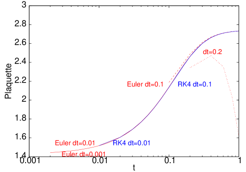
Figure 1: The effect on the flow of changing integrator and $dt$. For $dt<0.2$ the difference between integrators is negligible, especially with increasing $t$. For $dt\geq 0.2$ the integrator wanders off from the true solution.

Figure 2: The integrated autocorrelation time estimated for ${\cal E}(t)$ computed from the Wilson operator for several data sets. The autocorrelations increase very rapidly with flow time before running out of statistics.

One technical issue has to do with the integration of the flow equations. We tested both the Euler integrator and the fourth-order Runge Kutta (RK4) integrator. In Figure 1 we show the evolution of the plaquette under the flow when it is integrated using each of these methods for one fixed configuration. As shown, both integrators perform well even for $dt=0.1$. Note that with the Euler integrator and $dt=0.1$ the first integration step has larger errors than the later steps. Such self-repair is seen also with a finer time step of $dt=0.01$. With the Euler integrator one sees a failure of this self-repairing mechanism when $dt=0.2$. The observation that the free configuration is an attractor of the map in eq. (1) serves to explain both self-repair and its failure. The fact that there is an attractor with a finite basin of attraction is the reason for self-repair, with the global errors being smaller than the ${\cal O}(t^{2})$ predicted by a local analysis. Its failure occurs for sufficiently coarse $dt$, when the flow falls outside this basin of attraction. RK4 is generally more stable, but even so, its global error is smaller than local analysis would lead us to believe. We used RK4 with $dt=0.01$, but checked the results statistically by changing $dt$ by a factor of 4 either way. We found that the statistical uncertainty in the measurement of flow times is larger than any effect of the evolution.

The statistical properties of the measurement of ${\cal E}(t)$ under evolution in flow time are also of interest. Since our measurements are separated by 10 or 20 MD trajectories, at $t=0$ they are quite decorrelated. However, as the flow integrates information over successively larger volumes, one expects autocorrelations to grow with flow time. We quantify the autocorrelations in terms of the integrated autocorrelation time, $\tau_{\rm int\/}$, which is defined in terms of an autocorrelation function of the measurements $C(s)$ as

$$\tau_{\rm int\/}=1+2\int_{0}^{\infty}ds\,C(s),$$ (9)

where $s$ is the separation between the measurements. In Figure 2 we show $\tau_{\rm int\/}$ for ${\cal E}(t)$ as a function of the flow time, $t$. In accordance with expectations, this shows an initial rapid increase. The observed plateau in $\tau_{\rm int\/}$ is due to insufficient statistics; clearly for the set with $\beta=5.6$, the effective number of configurations decreases by a factor of around 20 when this plateau develops. Significantly more statistics would be needed to improve the measurement in this region, and decrease the estimate of the error in $\tau_{\rm int\/}$ elsewhere.

If the scaling of autocorrelations is physical, i.e., has a sensible continuum limit, then a natural way to compare flow times for different simulations would be to scale them by $w_{0}^{2}$ (or, equivalently, $t_{0}$). HMC simulations with fixed trajectory lengths have $\tau_{\rm int\/}$ scaling as the square of correlation lengths hmc . Since flow time also scales as the square of lengths, one should expect $\tau_{\rm int\/}\simeq w_{0}^{2}$. Figure 2 illustrates that this scaling is not present in the initial state, but develops fairly early during the flow and is a good first approximation to the observation. It would take significantly improved statistics to study the remaining deviations. The physics result is simple: as the lattice spacing decreases, the statistics required to keep a constant error on the flow scale increases (roughly) as the inverse square of the lattice spacing.

IV Results

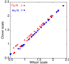
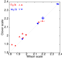
Figure 3: The comparison of Wilson flow scales determined using the Wilson (plaquette) or the clover operator. The scale is varied by changing both gauge coupling and the bare quark mass. Up triangles denote $\sqrt{t}_{0}/a$, down triangles are for $w_{0}/a$. The unfilled symbols show the direct measurements, and filled symbols the tree-level improved values. The panel on the left collects all our measurements, that on the right shows only the four smallest lattice spacings, by zooming into the dotted box shown at the left.

Figure 4: The pion mass in physical units as a function of the bare quark mass.

In Figure 3 we plot a flow scale obtained with the Wilson operator used for ${\cal E}(t)$ against the same scale obtained with the clover operator. If the two were equal, then the measurements would lie on the diagonal line. It has been observed before that the clover improvement changes the flow scale $\sqrt{t_{0}}$ quite significantly, as we verify again. The data set for the scale $w_{0}$ is significantly closer to the diagonal. Both of these scales are improved significantly by a tree-level improvement, at least on coarser lattice spacings: both sets of measurements are moved significantly closer to the diagonal line. However, as shown in the zoom in Figure 3, the improvement is marginal for $w_{0}$ at the smallest lattice spacings. This implies that any remaining finite lattice spacing corrections in $w_{0}$ are small. In view of this, we will use the tree-level improved value of $w_{0}$ to set the scale in the rest of the paper. We see that the range of lattice spacings we scan covers a factor of four from the coarsest to the finest.

We apply this scale setting first to re-examine the pion mass measurement. Our measurements of $m_{\pi}$ in lattice units are given in Table 1. We plot $m_{\pi}$ in units of $w_{0}$ in Figure 4. It is clear from the figure that the range of pion masses explored in this study covers a factor of four from the largest to the smallest. Given the rapid variation of $a/w_{0}$ and $m_{\pi}w_{0}$ with the bare coupling and the bare quark mass, it is useful to trade the bare parameters for these two.

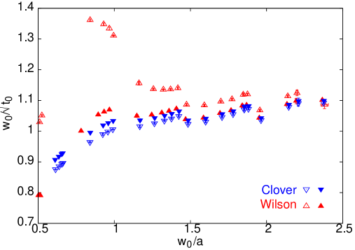
Figure 5: The ratio of the scales $w_{0}/\sqrt{t_{0}}$ for all the bare couplings and quark masses studied. At the smallest lattice spacings the ratio from Wilson (up triangles) and clover (down triangles) operators, for both direct (unfilled symbols) and tree-level improved (filled symbols) scales tend to the same value.

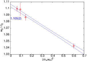
Figure 6: (a) Variation of $w_{0}/\sqrt{t_{0}}$ with the lattice spacing at fixed $m_{\pi}w_{0}\simeq 0.3$. The systematics of the continuum extrapolation is discussed in the text. (b) Variation of $w_{0}/\sqrt{t_{0}}$ with $m_{\pi}w_{0}$ at the smallest bare coupling. Chiral logs chirallog are not visible at this precision.

Since both the scales $\sqrt{t_{0}}$ and $w_{0}$ are physical, the ratio ${\cal R}=w_{0}/\sqrt{t_{0}}$ is expected to tend to a good limit as the lattice spacing decreases. In Figure 5 we show the dependence of this ratio on the lattice spacing (given in units of the tree-level corrected value of $w_{0}$). At the smallest lattice spacing which we have examined ($w_{0}/a\simeq 2.4$), ${\cal R}\simeq 1.100\pm 0.003$. For 2+1+1 flavours of staggered quarks milcscale we deduce ${\cal R}\simeq 1.21\pm 0.01$, where the error is estimated conservatively by neglecting covariance of the numerator and denominator. Since the statistical errors in $\cal R$ are small, the difference is significant. In a direct computation we checked that in the pure gauge theory, when $w_{0}/a\simeq 2.4$, the ratio ${\cal R}=1.012\pm 0.005$ (this is consistent with results presented in flowqcdscale ). The ratio clearly depends on the number of flavours of quarks.

$\cal R$ also depends on the lattice spacing and the quark mass, as shown in Figure 6. At fixed renormalized quark mass, $m_{\pi}w_{0}\simeq 0.3$ we have tried a quadratic extrapolation to the continuum. Using the data points on the four finest lattices, the continuum extrapolated ratio is $1.101\pm 0.003$. A fit using the quartic term gives the extrapolated value $1.11\pm 0.01$. If one uses only the three finest lattices, then the continuum extrapolation gives ${\cal R}=1.108\pm 0.007$. We put these observations together and quote a continuum extrapolated value

$${\cal R}=\frac{w_{0}}{\sqrt{t_{0}}}=1.106\pm 0.007({\rm stat\/})\pm 0.005({\rm syst}).$$ (10)

Following sommer , we define a measure of the slope with respect to the lattice spacing as

$$S^{a}_{\cal R}=\frac{{\cal R}(a=w_{0}/1.75)}{{\cal R}(a=0)}-1\simeq 14\%.$$ (11)

This is significantly larger than the results which can be reconstructed from values for other slopes quoted for $N_{f}=2$ clover improved Wilson fermions in sommer . At this time we are unable to comment on what combination of factors most influences this difference: the nature of the sea quarks, the value of $m_{\pi}$, or technical issues in comparing slopes of slightly different quantities sommer .

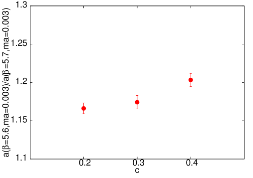
Figure 7: The ratio of the lattice spacings for two different sets of bare parameters depends on the renormalization scheme, i.e., the choice of $c$, through $w_{0}(c)$.

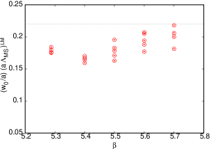
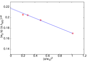
Figure 8: The ratio $w_{0}\Lambda_{\overline{\scriptscriptstyle MS}}$ extracted using the Lepage-Mackenzie scheme for computing $(a\Lambda_{\overline{\scriptscriptstyle MS}})^{LM}$. The first panel shows all our simulation results plotted as a function of the bare coupling $\beta$. The next panel shows the results for fixed $m_{\pi}w_{0}\simeq 0.3$ and a quadratic continuum extrapolation.

It is known that $w_{0}$ is more strongly dependent on the quark mass than $t_{0}$ sommer . A roughly linear dependence of both the scales with the renormalized quark mass has been observed before over a range of $m_{\pi}w_{0}$ similar to that explored here. Figure 6 shows this linear behaviour of the ratio $w_{0}/\sqrt{t_{0}}$. An extrapolation to the chiral limit as $m_{\pi}^{2}w_{0}^{2}$ at our smallest bare coupling yields $w_{0}/\sqrt{t_{0}}=1.105\pm 0.002$ Using the $N_{f}=2$ value for $w_{0}$ above. Defining an effective slope parameter

$$S^{m}_{\cal R}=\frac{{\cal R}(m_{\pi}w_{0}=0.45)-{\cal R}(m_{\pi}w_{0}=0.30)}{{\cal R}(m_{\pi}w_{0}=0.45)+{\cal R}(m_{\pi}w_{0}=0.30)}\,,$$ (12)

our observations give $S^{m}_{\cal R}\simeq 2$%. This is compatible with the change reported with two flavours of clover improved Wilson quarks in sommer .

Since the parameter $c$ determines the value of the running coupling eq. (6), one may use the RG-flow of the coupling to examine the $c$-dependence of $w_{0}(c)$. Define a measure of the change in $w_{0}(c)$ through

$$S_{c}=\frac{w_{0}(c=0.4)/a-w_{0}(c=0.2)/a}{2w_{0}(c=0.3)/a},\qquad(a{\rm\ fixed\/}).$$ (13)

On our finest lattice, we find $S_{c}\simeq 0.1$. The same measure with $t_{0}$ gives about 0.2. The formal two-loop expression for the running of $g_{R}$ in eq. (6) yields $S_{c}\simeq 0.3$. Since the renormalized couplings obtained for these $c$ are large, the two-loop beta function does not run the coupling reliably, so one should take the last number only as indicating that such large changes in scale are natural when changing $c$.

It is more interesting to ask whether the ratio of lattice spacings at two different bare couplings and quark masses is independent of the choice of $c$, when each of these is given in units of $w_{0}$. Ideally, of course, such a ratio should not change with $c$. In Figure 7 we show that, in fact, there is some residual dependence on the parameter $c$. Take the case where this ratio is close to 1.175 for $c=0.3$. The change in this ratio of lattice spacings for variation of $\Delta c=0.2$ around $c=0.3$ is 3% of the central value. While not ideal, this change is rather small. Presumably this uncertainty in the scale setting is due to remaining lattice spacing corrections. It would be interesting in the future to perform this comparison at smaller lattice spacings.

Measurements of plaquettes can also be converted to a scale using the methods of lm . Since the scale setting by the flowed plaquette suffers from significant lattice spacing effects at flow times $w_{0}^{2}$, necessitating the various corrections which we have explored, it may be suspected that these effects could be larger at flow time $t=0$. These are partly taken into account by corrections suggested in ehk . In Figure 8 we show the dimensionless ratio $w_{0}\Lambda_{\overline{\scriptscriptstyle MS}}$ obtained by a comparison of this scale with the flow scale $w_{0}/a$. In the second panel of Figure 8, we show the ratio $w_{0}\Lambda_{\overline{\scriptscriptstyle MS}}$ at fixed pion mass, $m_{\pi}w_{0}\simeq 0.3$ as a function of the lattice spacing. One sees a strong, nearly quadratic, lattice spacing dependence, albeit with a slope smaller than $S^{a}_{\cal R}$. A quadratic extrapolation to the continuum limit gives $w_{0}\Lambda_{\overline{\scriptscriptstyle MS}}=0.218\pm 0.001$, where the error is statistical only. It is interesting to compare this indicative number to the value for $N_{f}=2$ clover fermions. We take $\Lambda_{\overline{\scriptscriptstyle MS}}=257\pm 26$ MeV as quoted in alpha , and combine it with the value of $w_{0}$ reported with $N_{f}=2$ clover fermions sommer , to get $w_{0}\Lambda_{\overline{\scriptscriptstyle MS}}=0.23\pm 0.03$.

V Conclusions

We have reported on investigations of the Wilson flow scales $\sqrt{t_{0}}$ and $w_{0}$ in QCD with two flavours of naive staggered quarks. Our investigations cover a wide range of lattice spacings (a factor of about 4) and pion masses (also a factor of about 4). We found that the scale $w_{0}$ has smaller lattice spacing artifacts than $\sqrt{t_{0}}$. One consequence of this is that tree-level improvement of the former has smaller effect than in the latter. In most of this paper we have used tree-level improved measurements of $w_{0}$ obtained from the clover operator as the object to set the scale by.

We found an interesting approximate scaling of the autocorrelations of the basic measurement $\langle{\cal E}(t)\rangle$. The integrated autocorrelation time increases with $t$ before saturating. The scaling implies that keeping the error in measurements of $w_{0}$ fixed in the continuum limit may require the statistics to grow as the inverse square of the lattice spacing.

We found that the ratio ${\cal R}=w_{0}/\sqrt{t_{0}}=1.100\pm 0.003$ when $w_{0}/a\simeq 2.4$. A continuum extrapolation at fixed $m_{\pi}w_{0}\simeq 0.3$ gave ${\cal R}=1.106\pm 0.007({\rm stat\/})\pm 0.005({\rm syst})$. Comparison with results for the pure gauge theory, and with $N_{f}=2+1+1$ reveals a dependence of $\cal R$ on $N_{f}$. The the compilation of sommer also shows this trend for staggered quarks, but not for Wilson quarks. For $N_{f}=2$ clover improved Wilson quarks, the value of $\cal R$ is different from our determination sommer .

The dependence of the scale $w_{0}(c)$ on $c$ is large; this is natural since $c$ enters linearly in the definition of $g_{R}^{2}$, which depends nearly logarithmically on the scale $w_{0}(c)$. In principle, this should not change the ratio of two lattice spacings. However, we found a mild (3%) dependence of the ratio of two lattice spacings on $c$. The effect is small enough that one suspects it is due to lattice spacing dependences which are not absorbed into the tree-level improvement of $w_{0}$.

By using our data sets to determine the scale via the Lepage-Mackenzie prescription lm we found that it has large lattice spacing corrections. However, with our data we tried a simple continuum extrapolation at fixed $m_{\pi}w_{0}\simeq 0.3$, and found $w_{0}\Lambda_{\overline{\scriptscriptstyle MS}}=0.218\pm 0.001$. If one then uses the ALPHA collaboration’s value $\Lambda_{\overline{\scriptscriptstyle MS}}=257\pm 26$ MeV for $N_{f}=2$, then one is led to the conclusion that for naive staggered quarks $w_{0}=0.17\pm 0.02$ fm. This error is purely statistical, and dominated by the statistical error in the determination of $\Lambda_{\overline{\scriptscriptstyle MS}}$.

Acknowledgements: These computations were performed with the Cray X1 and IBM Blue Gene/P installations of the ILGTI in Mumbai, and with the Cray XK6 installation of the ILGTI in Kolkata.

References

- (1) M. Lüscher, J. H. E. P. 1008 (2010) 071 [arxiv:1006.4518], J. H. E. P. 1403 (2014) 092; M. Lüscher, arxiv:1101.0962,
- (2) R. Narayanan and H. Neuberger, J. H. E. P. 0603 (2006) 064 [hep-th/0601210]; R. Lohmayer and H. Neuberger, PoS LATTICE2011 (2011) 249 [arxiv:1110.3522].
- (3) S. Borsanyi et al., J. H. E. P. 1209 (2012) 010 [arxiv:1203.4469].
- (4) R. Sommer, PoS LATTICE2013 (2014) 015 [arxiv:1401.3270]; R. Sommer and U. Wolff, Nucl. Part. Phys. Proc. 261–262 (2015) 155 [arxiv:1501.01861].
- (5) A. Francis et al., Phys. Rev. D91 (2015) 096002 [arxiv:1503.05652]; M. Asakawa et al., arxiv:1503.06516.
- (6) M. Bruno and R. Sommer, PoS LATTICE2013 (2014) 321 [arxiv:1311.5585].
- (7) R. Horsley et al., PoS LATTICE2013 (2014) 249 [arxiv:1311.5010].
- (8) R. J. Dowdall et al., Phys. Rev. D88 (2013) 074504 [arxiv:1303.1670]; A. Bazavov et al.(MILC) arxiv:1503.02769.
- (9) I. Montvay and G. Muenster, Quantum Fields on a Lattice, Cambridge University Press (1994).
- (10) Z. Fodor et al., J. H. E. P. 1409 (2014) 018 [arxiv:1406.0827].
- (11) Z. Fodor et al., J. H. E. P. 1211 (2012) 007 [arxiv:1208.1051].
- (12) S. Gottlieb et al., Phys. Rev. D38 (1988) 2235; K. M. Bitar et al., Phys. Rev. D42 (1990) 3794; F. R. Brown et al., Phys. Rev. Lett. 67 (1991) 1062.
- (13) S. Gupta, Nucl. Phys. B 370 (1992) 741.
- (14) O. Bär and M. Golterman, Phys. Rev. D89 (2014) 034505 [arxiv:1312.4999].
- (15) G. P. Lepage and P. B. Mackenzie, Phys. Rev. D48 (1993) 2250 [hep-lat/9209022].
- (16) R. G. Edwards et al., Nucl. Phys. B 517 (1998) 377.
- (17) M. Della Morte et al., J. H. E. P. 0807 (2008) 037.