3D-2D transition in mode-I fracture microbranching in a perturbed hexagonal close-packed lattice

Abstract

Mode-I fracture exhibits microbranching in the high velocity regime where the simple straight crack is unstable. For velocities below the instability, classic modeling using linear elasticity is valid. However, showing the existence of the instability and calculating the dynamics post-instability within the linear elastic framework is difficult and controversial. The experimental results give several indications that the microbranching phenomenon is basically a three-dimensional phenomenon. Nevertheless, the theoretical effort has been focused mostly in two-dimensional modeling. In this work we study the microbranching instability using three-dimensional atomistic simulations, exploring the difference between the 2D and 3D models. We find that the basic 3D fracture pattern shares similar behavior with the 2D case. Nevertheless, we exhibit a clear 3D-2D transition as the crack velocity increases, while as long as the microbranches are sufficiently small, the behavior is pure 3D-behavior, while at large driving, as the size of the microbranches increases, more 2D-like behavior is exhibited. In addition, in 3D simulations, the quantitative features of the microbranches, separating the regimes of steady-state cracks (mirror) and post-instability (mist-hackle) are reproduced clearly, consistent with the experimental findings.

I Introduction

Over the last decades, the dynamic instability in mode-I fracture has been extensively studied review . These findings deviate from the two-dimensional classic model for mode-I fracture with a single crack that propagates in the midline of the sample, based on linear elasticity fracture mechanics (LEFM) freund . This classic theory, which lacked a supplemental criteria for instability, predicts that a single crack will accelerate to a terminal velocity, which for mode-I fracture is the Rayleigh surface wave speed, $c_{R}$. In fact, as long as a single crack does exist, the crack obeys LEFM predictions review_mid ; review_new . However, the experiments find that at a much lower velocity ($\approx 0.36-0.42c_{R}$, for a short review, see for example adda_bedia ), a dynamic instability occurs, and small microbranches start to appear nearby the main crack marder_jay1 ; fineberg_sharon1 ; fineberg_sharon2 ; fineberg_sharon3 ; fineberg_sharon5 . The additional energy that has to be spent in creating the new surfaces prevents the crack from accelerating to the theoretical terminal velocity. LEFM-based universal criteria for branching yoffe ; eshelby fail to describe the instability, predicting a much higher critical velocity than in reality. Moreover, when the small microbranches appear at $v\geqslant v_{cr}$, they present a clear 3D nature. However, when enlarging the driving displacement, the small microbranches reunite, creating 2D patterns (right before macro-branches appear), especially in PMMA fineberg_sharon1 ; fineberg_sharon2 ; fineberg_sharon3 ; fineberg_sharon5 .

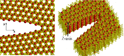
Figure 1: (color online) A snapshot of the (same) crack tip in steady-state crack using a perturbed hexagonal close-packed (hcp) lattice, from different viewing angles. Each atom shares 12 nearest neighbors, defining “bonds” that connect each other by a force law, and is allowed to move in all three coordinates. The crack creates mirror-like pattern. The left snapshot is a clear XY-plan view while the right has a slight tilt, showing how deep the system is.

Lattice models reproduce the existence of steady state cracks slepyan ; slepyan2 , and via a standard linear stability analysis, they predict the existence of a critical velocity, when the steady-state cracks becomes linearly unstable marderliu ; kess_lev3 ; pechenik ; shay1 ; shay2 . This critical velocity is found to be strongly dependent on the details of the inter-atomic potential, such as the degree of smoothness of the potential (as it drops to zero), or the amount of dissipation. Simple simulations that use these same potentials succeed in reproducing the steady-state regime, yielding the exact point of instability, and in reproducing the lattice models results, but fail to describe the behavior in the post-instability regime fineberg_mar ; shay1 . The early efforts on using a binary-alloy model for modeling brittle amorphous materials failed to achieve steady-state cracks at all falk , although more recent attempts have succeeded in yielding propagating cracks procaccia1 ; procaccia2 .

Recent studies using Zachariasen’s zachariasen 2D continuous random network model (CRN) of amorphous materials, a model that also has recently received experimental support from direct imaging of 2D silica glasses tem1 , were used in describing the microbranching instability shay3 (using ${\cal O}\left(10^{4}\right)$ 2D particle mesh). The simulations reproduced qualitatively both the regime of steady-state propagating cracks and the fracture patterns of the microbranches. In addition, using perturbed lattice models, generated by adding a small amount of disorder to the bond lengths, supplemented by an additional 3-body force-law which penalize rotation of the bonds away from the natural directions of the lattice, produces similar results shay4 . Larger scale simulations (${\cal O}\left(10^{6}\right)$ particles) using GPU computing yields various qualitative and quantitative results of post-instability behavior such as a sharp transition between the regime of steady-state and microbranching, the increase of the derivative of the electrical resistance across the crack with respect to time (which correlates experimentally with the crack velocity), the correct branching angle and also the power-law behavior of the branch shapes shay5 . All of the theoretical models that were mentioned above employed a 2D description of the problem.

The large scale simulations allow us for the first time to perform three-dimensional (3D) simulations, attacking the microbranching phenomenon which is, at its heart, a 3D phenomenon review ; fineberg_sharon2 ; kolvin , by taking the ${\cal O}\left(10^{4}\right)$ particle mesh and adding a third dimension with $N_{Z}\approx 100$. The two basic questions that we address using our 3D simulations are:

1. Checking the reliability of the previous 2D simulations, investigating how well the 2D description reproduces the behavior of the more realistic 3D models;

2. Studying for the first time the direct 3D experimental features of the microbranches, which have not previously been modeled.

We note that several 3D fracture molecular-dynamics simulations, containing large numbers of atoms, have been studied previously using different potentials (for example, see abraham1 ; abraham2 ; review3d ), but intensive study concerning the features of the 3D instability and the features of the microbranches have not yet been studied. It is important to note that atomistic simulations cannot reproduce the fracture patterns on the real physical length scales, of the experiments. However, they try to reproduce scaled results and scaled structures of the real fracture length scales.

II Model and General Methodology

Our simulations consist of $\approx 3\cdot 10^{6}$ atoms, which include $1.7\cdot 10^{7}$ bonds (central force-laws), and $\approx 3.4\cdot 10^{7}$ 3-body interactions (see appendix B for the exact parameter of the 3-body potential that was used). These simulations can be performed in reasonable run times by using parallel GPU computing (see appendix C).

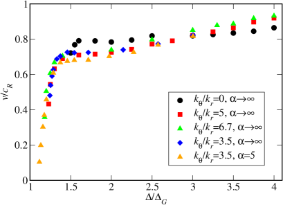
Figure 2: (Color online) The $v(\Delta)$ curve of the perturbed hcp with different values of 2-body and 3-body force laws. With a finite value of $\alpha$ and $k_{\theta}/k_{r}$, the velocity gap shrinks dramatically, yielding the correct experimental behavior.

We used a perturbed hexagonal close-packed (hcp) structure, which is a 3D extension of the 2D perturbed hexagonal lattice that was studied in shay4 ; shay5 . As in our 2D studies, the interactions are taken to be only between nearest-neighbors in the unperturbed hcp lattice, with an in-plane lattice constant of $a=4$ and $c=\sqrt{8/3}a$ (see Fig. 9 in appendix A). Every atom has 12 closest neighbors. We add a small amount of disorder to the bond lengths, $a_{i,j}=(1+\epsilon_{i,j})a$ where $\epsilon_{i,j}\in[-b,b]$, and $b$ is constant, and in this work is set to $b=0.1$ (for the system shape, see Fig. 10 in appendix B). In most of our simulations, we employed a piecewise-linear radial force law (in this work, $k_{r}=1$) between the initially neighboring atoms. However, in some of them we used a more physical smooth force law, using a smoothness parameter $\alpha$, which when $\alpha\to\infty$ reproduces the piecewise-linear model (see appendix B). In addition, we add a 3-body potential and Kelvin type viscosity, as described in detail in our 2D lattice studies shay4 ; shay5 . We relax the system, and then we strain the lattice under a mode-I tensile loading with a given constant strain grip boundary condition corresponding to a given driving displacement $\pm\Delta$ (which is normalized relative to the Griffith displacement $\Delta_{G}$) of the edges and seed the system with an initial crack. For a detailed discussion regarding the model and the governing equations, see appendixes A andB. The crack then propagates via the same molecular dynamics Euler scheme (the simulations were always stable using a reasonable value of $dt$, so we have not needed any more sophisticated numerical schemes). In Fig. 1 we present close-in snapshots of the (same) crack tip in a steady-state crack from different viewing angles. We can see that at low driving displacement the crack is actually 2D in nature.

III Microbranching instability in 3D-Perturbed Lattice

The crack velocity $v$ (which we normalize to the Rayleigh wave speed $c_{R}$) increases with $\Delta/\Delta_{G}$ (see Fig. 2). We define the Rayleigh wave speed here as that calculated from $c_{l}$ and $c_{t}$ (the longitude and the transverse wave speeds) in the XY-plane ($(0001)$ in the crystallographic notation), which is the major fracture surface in our simulations (there is a symmetry along the Z-axes in steady-state cracks, see appendix D). We can see that using a perfect non-perturbed lattice (in these simulations we used also $k_{\theta}=0$, in addition to $b=0$, but this result is valid for all value of $k_{\theta}$), we get a (non-physical) velocity gap (like in 2D marderliu ; kess_lev3 ; pechenik ; shay1 ), in which slow cracks are prohibited. However, adding disorder and the 3-body force-law, the velocity gap shrinks, and by using a finite value of $\alpha$, the velocity gap shrinks dramatically with steady-state cracks in almost zero velocities, yielding the correct experimental behavior review .

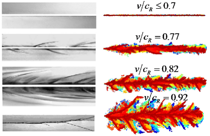
Figure 3: (Color online) A XY plan view of the experimental microbranching phenomenon in PMMA taken from fineberg_sharon2 ; fineberg_sharon5 (left) for increasing driving displacement. In color (right) we see our simulations XY plan view, where the color denotes the Z-location of the broken bonds (dark red for top edge and dark blue for bottom edge). We can see that despite the quite noisy simulations, in general the qualitative picture is quite good. The upper picture yields a mirror-like steady-state crack and is valid for all $v/c_{R}\leqslant 0.7$.

In. Fig. 3 we show several microbranching patterns (top views), both experimental (in PMMA) and from our 3D simulations using $k_{\theta}/k_{r}=5$ (where the color denotes the Z-location). The broken bonds are plotted in the fractured system, and their Z-location can be associated with the color, where dark red represents the top edge and dark blue for bottom edge. We see that below the critical velocity, in the regime of steady-state cracks, the crack has a “mirror” surface. Increasing the driving displacement, small microbranches appear nearby the main crack, while the size of the microbranches increases dramatically with the driving, yielding at first a “mist” surface and with large $\Delta$, a “hackle” surface. Despite the noisy results (due to the relatively small size of the simulations), the pictures are qualitatively quite similar to the experimental findings, at least in the sense that the microbranches increase dramatically with the driving displacement, yielding eventually large macro-branches (in the simulations, a “macro-branch” is a branch that reaches the end of the sample, like in the experiments, on a different length scale). A quantitative (scaled) overview is presented in Figs. 4-5. We note that without a 3-body force-law we do not get the microbranching pattern, but rather a cleavage-like behavior (with or without the presence of disorder). Using too strong a 3-body force law ($k_{\theta}/k_{r}=6.7$), yields microbranches that propagate in straight lines with the natural angle of the lattice ($60\degree$), which is again non-physical.

The transition between the regime of steady-state cracks and the post-instability side-branching regime is very sharp in the 3D simulations. In Figs. 4-5 we present two quantitative parameters that demonstrate this sharp transition (in the small box there is a zoomed picture of the transition area). In Fig. 4 the total number of broken bonds as a function of the crack velocity is displayed. In the small velocity regime, only the bonds necessary for yielding a single main crack are broken. Beyond the critical velocity, the number of broken bonds increases linearly, as in the experiments fineberg_sharon2 , and broadly similar (although much sharper here) to what is seen in the hexagonal perturbed 2D lattice shay5 .

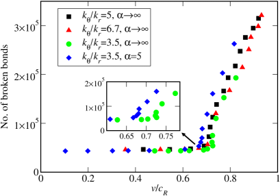
Figure 4: (Color online) The total number of broken bonds as a function of the crack velocity (the constant number of bonds in the small velocity regime represents the broken bonds of the main crack). A clear transition between the steady-state regime and microbranching behavior can be seen. In the small box there is a zoomed picture of the transition area.

In Fig. 5 we measure $\delta y$, the width of the microbranching region, as a function of the crack velocity (see definition inside Fig. 5). $\delta y$ is a second measure of the size of the microbranches. As above, a sharp transition can be seen between the single crack and microbranching regimes. We note that using the piecewise-linear force law, the critical velocity $v_{\mathrm{cr}}$ seems to be very close to the Yoffe criterion (which is $\approx 0.73c_{R}$). But, as we showed previously in 2D, the quantitative value of the $v_{\mathrm{cr}}$ can be controlled via the inter-atomic potential parameters, such as $\alpha$ and $\eta$ (see appendix B for explicit definitions of these parameters) kess_lev3 ; shay1 ; shay5 . We can see that using a finite value of $\alpha$, the critical velocity decreases (see the small boxes in Figs. 4-5 for a given $k_{\theta}$), to the exact value of the 2D simulations; in $\alpha\to\infty$ we reproduce the 2D critical velocity $v_{\mathrm{cr}}\approx 0.73c_{R}$ (see Fig. 7 in pechenik ), while also with $\alpha=5$ we reproduce the 2D value, $v_{\mathrm{cr}}\approx 0.68c_{R}$ (see Fig. 4(a) in shay1 ). That means that the critical velocity is not universal and is potential-dependent. Thus, for example we can vary the values of $\alpha$ and $\eta$ to reproduce the exact experimental critical velocity of a given material, very much like we did in 2D shay1 ; shay2 . In both Fig. 4 and 5, the results appear insensitive to the exact value of $k_{\theta}$, despite the fact that the microbranches in the two cases appear different.

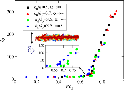
Figure 5: (Color online) The width of the fracture region as a function of the crack velocity. A clear transition between the steady-state regime and microbranching behavior can be seen. In the small box there is a zoomed-in picture of the transition area.

In addition, we can cut thin horizontal slices from the XY fracture pattern, yielding 2D patterns and compare them to pure 2D fracture patterns shay4 . In Fig. 6 we present two fracture patterns of a 2D perturbed hexagonal lattice and and two 2D slices of the 3D hcp perturbed lattice, one for relatively small driving and one for large driving displacement. We can see despite the relatively large noise (resulting from the breaking of one or few bonds) that characterizes the 3D simulations, the patterns are quite similar to pure 2D simulations for small driving displacement. This fact is encouraging and supports the assumption that for at least some features (e.g., XY-plane features of the microbranches), the 2D studies are relevant. However, for large driving displacement, the 3D patterns look rather different from the 2D patterns, though the fracture-pattern is still much more developed at large driving displacements. Nevertheless, we note that different horizontal slices of the same 3D fracture pattern (for different Z) yield different patterns. This fact indicates that for the 3D regime, as long as the microbranches are sufficiently small, there is no symmetry along the Z-axis. Note that the driving displacement $v/c_{R}$ required to produce a given amount of side-branching is much greater than in 2D, since out of plane bonds are being broken as well.

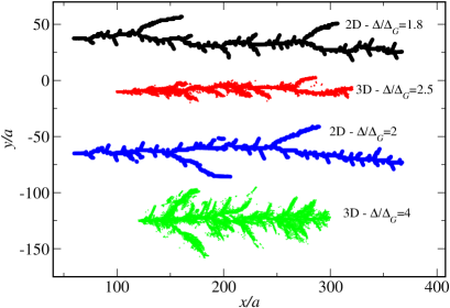
Figure 6: (Color online) A comparison between the fracture pattern (in lattice scale units) of a pure 2D perturbed hexagonal simulation and thin slices of the 3D fracture pattern using our perturbed hcp lattice. Despite the greater noise of the 3D simulations, the patterns look quite similar. The 2D patterns are taken from shay4 .

IV The 3D-2D transition

Moreover, we can compare our 3D simulations to the 3D experimental properties of the microbranches. Experimental post-mortem pictures of the XZ-plane of the fractured surface by Sharon & Fineberg fineberg_sharon2 reveal that nearby the origin of instability, the microbranches are localized in the Z-axis. At large velocities, the microbranches merge, creating a Z-plane quasi-symmetric pattern, yielding a 3D-2D transition review ; fineberg_sharon2 ; fineberg_sharon3 ; fineberg_sharon5 . In PMMA (as opposed to glasses or gels), nice symmetric “2D”-like strips are created in association with the largest microbranches fineberg_sharon2 .

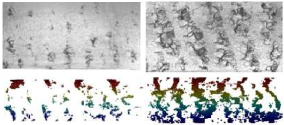
Figure 7: (Color online) Top row: A XZ-plane view of the experimental microbranching phenomenon in PMMA of Sharon & Fineberg experiments (which are taken from fineberg_sharon2 ), along with simulations results (where the color denotes the Z-location of the broken bonds for presentation reasons), for small driving on the left, and for large driving displacement on the right. Bottom row: The simulational XZ plane view. We see that very much like the experiments, at small driving displacement the microbranching is “3D” and for large driving displacement, the microbranches are “2D” in character.

In Fig. 7 we present two experimental pictures of XZ-plane of the fracture surface that demonstrates the 2D-3D transition in PMMA, taken from Ref. fineberg_sharon2 . Below, we depict XZ slices taken at a constant distance from the main crack (relative to the Y-axis) of our 3D simulations (the pictures from the main crack plane itself are too noisy, due to our finite size simulations). We see that the fracture patterns looks surprisingly similar. At small driving displacement ($\Delta/\Delta_{G}=2.5$ in the simulations), right beyond the critical velocity, the microbranches are localized in the Z-directions, yielding purely 3D behavior in both the experiments and the simulations. Increasing the driving displacement further ($\Delta/\Delta_{G}=4$ in the simulations), the microbranching increases in the Z-direction from top to bottom of the sample, yielding a 2D type behavior. The periodic stripes structure is a result of the periodic microbranches in the XY-plane (Fig. 3) fineberg_sharon1 . After the onset of branching, the energy flowing into the crack tip is divided between the main crack and the daughter cracks. The daughter cracks, which compete with the main crack, have a finite (similar) lifetime, because the main crack can outrun them and screen the daughter cracks from the surrounding stress field. The daughter cracks then die and the energy that had been diverted from the main crack returns. The scenario then repeats itself, causing the branching pattern to be more or less, periodic.

As a matter of fact, these large microbranches result from the merging of several small microbranches, as we can see carefully in Fig. 7 (there is not a perfect symmetry along the Z-axis; for different Z, the microbranch propagates different distances). This behavior shares similar features with recent experimental work kolvin .

We can now quantify this 2D-3D transition (of course in normalized units). Looking carefully in the PMMA experimental results, we can see that the region of instability, $v=v_{cr}\approx 340\mathrm{m/s}$ (Fig. 11(a) in fineberg_sharon2 ) is quite differ from the point of 2D-3D transition, $v\approx 550\mathrm{m/s}$ (Fig. 19 in fineberg_sharon2 ), ensuring the fact that at first (near $v\approx v_{cr}$) the microbranches are “3D”, while only for larger velocities, they become “2D”. In Fig. 8, we plot the width of the largest microbranch (in the Z-direction) in the 3D simulations for a given $\Delta/\Delta_{G}$, along with the total number of broken bonds (from Fig. 4), both of them are normalized to their largest value. We plot them both as a function of $\Delta/\Delta_{G}$ and not as a function of $v/c_{R}$, since the crack velocities are an output parameter (and in our simulations are much higher than the PMMA experimental results). For the experimental results, we used Fig. 17 in review for transferring the data from $v/c_{R}$ to $\Delta/\Delta_{G}$.

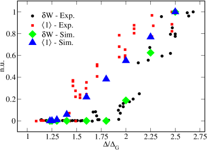
Figure 8: (Color online) A comparison between experimental and simulations results for the average length of microbranch and microbranch width (normalized to the maximal yielded value) as a function of the driving displacement (normalized to the Griffith value). The experimental data is taken from fineberg_sharon2 ; review .

We can see that the 3D simulations results are reproducing the 2D-3D transition almost perfectly. At $\Delta/\Delta_{G}\approx 1.3$, in both the experimental and the simulations results, small microbranches start to appear the main crack. Those microbranches are localized in the Z-direction, while only at $\Delta/\Delta_{G}\approx 1.8-1.9$, the width of the microbranches increases dramatically, yielding “2D-microbranches”, when several microbranches reunite, covering the whole Z-directions, yielding a 3D-2D transition.

V Summary and Future work

In conclusion, as long as we look in the XY-plane, the 3D simulations share similar features as the 2D simulations, and quantitative measures as to the total number of microbranches or the size of the opening of the microbranches as a function of crack velocity look the same. On the other hand, our current simulations also reproduce pure 3D features, especially the XZ-plane patterns, when the 3D-2D transition occurs. Thus, we believe that the lattice models and simulations offer a good theoretical framework for studying the microbranching instability, including the 3D effects. We are left with the following question. In 2D shay5 , enlarging the system allows quantitative study of the branches. How will behave the 3D system on a larger scale? The answers should be attainable within the scope of available supercomputers, using thousands of nodes, or tens of GPU’s.

Appendix A Generating the perturbed lattice

We start with a perfect ideal hexagonal close-packed (hcp) lattice, where $c=\sqrt{8/3}a$ (see Fig. 9) when each atom has 12 nearest neighbors, 6 in the XY-plane, (yielding a 2D hexagonal lattice) and 6 in the Z-direction (3 up and 3 down). As in the 2D-studies shay4 ; shay5 , we randomize the length of each “bond”, $a_{i,j}$:

$$a_{i,j}=(1+\epsilon_{i,j})a,\qquad i=1,2,\dots,n_{\mathrm{atoms}},j\in{\cal N}(i)$$ (1)

where $\epsilon_{ij}\in[-b,b]$, and $b$ is constant for a given lattice. In this work we set $b=0.1$ and $a=4$. ${\cal N}(i)$ refers to the nearest-neighbors of site $i$.

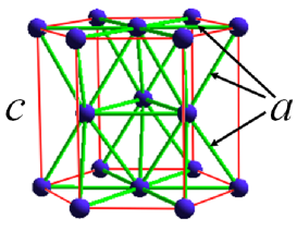
Figure 9: (color online) A diagram of the unit cell of the ideal hexagonal closed packed (hcp) lattice, where $c=\sqrt{8/3}a$. Each atom has 12 nearest neighbors, 6 in the XY-plane (reproducing the 2D hexagonal lattice).

Appendix B The equations of motion

In most of our calculations, between each two atoms there is a piecewise linear radial force (2-body force law) of the form:

$$\vec{f}^{r}_{i,j}=k_{r}k^{\prime}_{i,j}(|\vec{r}_{i,j}|-a_{i,j})\hat{r}_{j,i},$$ (2)

where:

$$k^{\prime}_{i,j}\equiv\theta_{H}\left(\varepsilon-|\vec{r}_{i,j}|\right).$$ (3)

The Heaviside step function $\theta_{H}$ guarantees that the force drops immediately to zero when the distance between two atoms $|\vec{r}_{i,j}|$ reaches a certain value $\varepsilon>a_{i,j}$ (the breaking of a “bond”). In this work we set $\varepsilon=a+1$. Alternatively to Eq. 3, we can use a smoother force law, which instead of a sharp failure at $|\vec{r}_{i,j}|=\varepsilon$, has a more realistic smooth transition wherein the force law drops to zero of the form kess_lev3 ; shay1 :

$$k^{\prime}_{i,j}\equiv\frac{1+\tanh[\alpha(\varepsilon-\vec{r}_{i,j})]}{1+\tanh(\alpha)}$$ (4)

where $\alpha$ is the smoothness parameter, such that when $\alpha\to\infty$ the force law reverts to the piecewise linear force law. The results in this paper refer to the piecewise linear model, unless mentioned otherwise.

In addition there is a 3-body force law that depends on the cosine of the angles between each set of 3 neighboring atoms, defined of course by:

$$\cos\theta_{i,j,k}=\frac{\vec{r}_{i,j}\cdot\vec{r}_{i,k}}{|\vec{r}_{i,j}||\vec{r}_{i,k}|},$$ (5)

that acts on the central atom (atom $i$) of each angle, and may be expressed as:

$$\vec{f}^{\theta}_{i,(j,k)}=k_{\theta}(\cos\theta_{i,j,k}-\cos\theta_{C})\frac{\partial\cos\theta_{i,j,k}}{\partial\vec{r}_{i}}\,k^{\prime}_{i,j}k^{\prime}_{i,k}\hat{r}_{i}=$$ (6)

$$k_{\theta}(\cos\theta_{i,j,k}-\cos\theta_{C})\left[\frac{\vec{r}_{i,j}+\vec{r}_{i,k}}{|\vec{r}_{i,j}||\vec{r}_{i,k}|}+\frac{\vec{r}_{j,i}(\vec{r}_{i,j}\cdot\vec{r}_{i,k})}{|\vec{r}_{i,j}|^{3}|\vec{r}_{i,k}|}+\right.$$

$$\left.\frac{\vec{r}_{k,i}(\vec{r}_{i,j}\cdot\vec{r}_{i,k})}{|\vec{r}_{i,j}||\vec{r}_{i,k}|^{3}}\right]k^{\prime}_{i,j}k^{\prime}_{i,k},$$

while the force that is applied on the other two atoms (atoms $j,k$) may be expressed as:

$$\vec{f}^{\theta}_{j,(i,k)}=k_{\theta}(\cos\theta_{i,j,k}-\cos\theta_{C})\frac{\partial\cos\theta_{i,j,k}}{\partial\vec{r}_{j}}k^{\prime}_{i,j}k^{\prime}_{i,k}\hat{r}_{j}=$$ (7)

$$k_{\theta}(\cos\theta_{i,j,k}-\cos\theta_{C})\left[\frac{\vec{r}_{k,i}}{|\vec{r}_{i,j}||\vec{r}_{i,k}|}+\frac{\vec{r}_{i,j}(\vec{r}_{i,j}\cdot\vec{r}_{i,k})}{|\vec{r}_{i,j}|^{3}|\vec{r}_{i,k}|}\right]k^{\prime}_{i,j}k^{\prime}_{i,k}$$

Of course, the forces satisfy the relation: $\vec{f}^{\theta}_{i,(j,k)}=-(\vec{f}^{\theta}_{j,(i,k)}+\vec{f}^{\theta}_{k,(i,j)})$. The 3-body force law drops immediately to zero when using a piecewise linear force law when the bond breaks (Eq. 3), or may be taken to vanish smoothly, using Eq. 4.

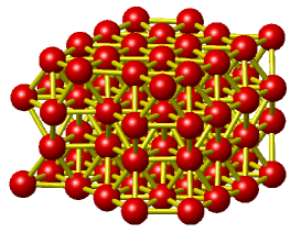
Figure 10: (color online) A small-scale perturbed hcp yielded by Eq. 1, after relaxing the system under Eqs. 2-9.

We note that in the 3D-case, there are a lot of possible angles between each set of 3 bonds. To shorten the run-times (the calculation of the 3-body force law is extremely time consuming), in most of our calculations, we do not include all the possible angles between triplets, but only 12 of them. We chose to take the 6 $60\degree$ angles inside the XY-plane (for reproducing the 2D-hexagonal problem that was studied before for $N_{z}=1$), and another 6 angles, three $60\degree$ that connect each atom with its two neighbors that are located in the upper parallel plane, and three angles in the lower parallel plane (For convenience, see Fig. 9). However, in some of our calculations, we used all the 24 $60\degree$ angles, while the results do not vary qualitatively, and the fracture patterns remain similar. There is a certain preferred angle $\theta_{C}$ for which the 3-body force law vanishes which is set to $\theta_{C}=\nicefrac{{\pi}}{{3}}$.

In addition, it is convenient to add a small Kelvin-type viscoelastic force proportional to the relative velocity between the two atoms of the bond $\vec{v}_{i,j}$ kess_lev1 ; kess_lev3 ; pechenik ; shay1 :

$$\vec{g}^{r}_{i,j}=\eta(\vec{v}_{i,j}\cdot\hat{r}_{i,j})\,k^{\prime}_{i,j}\hat{r}_{i,j},$$ (8)

with $\eta$ the viscosity parameter. The viscous force vanishes after the bond is broken, governed by $k^{\prime}_{i,j}$. The imposition of a small amount of such a viscosity acts to stabilize the system and is especially useful in the relatively small systems simulated herein.

The set of equations of motion of each atom is then:

$$m_{i}\vec{\ddot{a}}_{i}=\sum_{j\in 12\;nn}\left(\vec{f}^{r}_{i,j}+\vec{g}^{r}_{i,j}\right)+\sum_{j,k\in 12\;nn}\vec{f}^{\theta}_{i,(j,k)}+\sum_{j\in 24\;nn}\vec{f}^{\theta}_{j,(i,k)}.$$ (9)

In this work the units are chosen so that the radial spring constant $k_{r}$ and the atoms mass $m_{i}$ is unity.

After defining the steady-state optimal length of each bond $a_{i,j}$ by Eq. 1, we first relax the system under the equations of motion, Eqs. 2-9 with a small amount of viscosity, yielding the minimal-energy locations of the atoms in the lattice. In Fig. 10, we can see a small-scale 3D perturbed hcp using our model.

After relaxing the initial lattice, we strain the lattice under a mode-I tensile loading with a given constant strain corresponding a given driving displacement $\pm\Delta$ of the edges and seed the system with an initial crack. The crack then propagates via the same molecular dynamics Euler scheme using Eqs. 2-9.

Appendix C Parallelization by GPU computing

As mentioned in Secs. I and II, running 3D simulations, using approximately $3\cdot 10^{6}$ particles cannot reasonably be performed by a singe CPU, and thus force us to use multi-thread computing. We choose to use GPU computing, parallelizing the code via CUDA padon ; cooper , akin to what we implemented before in 2D shay5 . This kind of programing forces the programmer to use the different levels of memory carefully cooper , which makes possible achieving an acceleration up to $\approx 100$ faster than a regular $C$ code using a single CPU. This tool makes possible the simulation of millions of atoms in reasonable simulation times. See the appendix of Ref. shay5 for more implementation details. In our simulations, we used $132\cdot 310\cdot 70\approx 3\cdot 10^{6}$ particles ($N=65$ in the Slepyan model notation).

Appendix D The Rayleigh surface wave speed for hcp with $k_{\theta}\neq 0$ lattices

Since the models in this paper use a 3-body potential law (aside by the central two-body force law) with $k_{\theta}\neq 0$, we need to recalculate the Rayleigh wave speed $c_{R}$, which is the terminal velocity for mode-I fracture for different $k_{\theta}/k_{r}$. The most convenient way to calculate the Rayleigh wave speed is to calculate first the longitude (primary) $c_{l}$ and the transverse (secondary) $c_{t}$ wave speeds and then, to calculate the Rayleigh wave speed via the well-known formula achenbach :

$$\left(1-\frac{c_{R}^{2}}{c_{t}^{2}}\right)^{2}-4\left(1-\frac{c_{R}^{2}}{c_{l}^{2}}\right)^{\nicefrac{{1}}{{2}}}\left(1-\frac{c_{R}^{2}}{c_{t}^{2}}\right)^{\nicefrac{{1}}{{2}}}=0$$ (10)

Since in an hcp lattice, the sound velocities are inhomogeneous, yielding a different sound velocity for each direction, we defined that the relevant variables are the variables in the XY-plane, which is the major fracture plane, and thus, the crack velocities are normalized to the sound velocities in the XY-plane (which inside this plane, are homogeneous, as for a 2D hexagonal lattice). In this manner we define the Rayleigh wave speed in the XY-plane, by Eq. 10. We calculate $c_{l}$ and $c_{t}$ via measuring the wave velocities by initiating longitude and transverse small deformations in the end of the samples in the different lattices that we use in this study and then find $c_{R}$ via Eq. 10. The results are shown in Fig. 11, with the circles indicating the results with the only 12 $60\degree$ angles that were taken into account, and the triangles the results with all 24 $60\degree$ angles. The value of $k_{\theta}$ with all 24 $60\degree$ angles was chosen for reproducing the quantitative values of the model with only 12 $60\degree$ angles model.

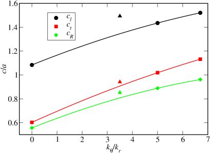
Figure 11: (Color online) The longitude and the transverse sound wave speeds along with the resulting calculated Rayleigh surface wave speed using Eq. 10 for the hcp lattice as a function of $k_{\theta}/k_{r}$. In circles there are the results with the only 12 $60\degree$ angles that were taken into count, while in the triangles, is the result with all 24 $60\degree$ angles.

We can see that for both lattices, the numerical value for the wave velocities using $k_{\theta}=0$ are very close to the 2D-values shay5 , as can be calculated analytically. For larger values of $k_{\theta}$, the different sounds velocities are higher ($\approx 10-15\%$) than the 2D velocities shay5 . In addition, we can see that the results for the sound velocities (in specific, $c_{R}$) with $k_{\theta}/k_{r}=3.5$ with all 24 $60\degree$ angles are very much alike the $k_{\theta}/k_{r}=5$ with only 12 $60\degree$ angles.

References

- (1) J. Fineberg and M. Marder, Phys. Repts. 313, 2 (1999).
- (2) L.B. Freund, Dynamic Fracture Mechanics, Cambridge University Press (1998).
- (3) E. Bouchbinder, J. Fineberg and M. Marder, Annu. Rev. Condens. Matter Phys. 1, 371 (2010).
- (4) E. Bouchbinder, T. Goldman and J. Fineberg, Rep. Prog. Phys. 77, 046501 (2014).
- (5) M. Adda-Bedia, J. Mech. Phys. Solids 53, 227 (2005).
- (6) J. Fineberg, S. P. Gross, M. Marder and H. L. Swinney, Phys. Rev. Lett. , 67, 457 (1991).
- (7) E. Sharon, S.P. Gross and J. Fineberg, Phys. Rev. Lett. 74, 5096 (1995).
- (8) E. Sharon and J. Fineberg, Phys. Rev. B 54, 7128 (1996).
- (9) E. Sharon and J. Fineberg, Philos. Mag. B 78, 243 (1998).
- (10) E. Sharon and J. Fineberg, Adv. Eng. Mat. 1, 119 (1999).
- (11) E.H. Yoffe, Philos. Mag. 42, 739 (1951).
- (12) J.D. Eshelby, in Inelastic Behavior of Solids, M. F. Kanninen, ed., (McGraw-Hill, New York, 1970).
- (13) M.L. Falk, Phys. Rev. B 60, 7062 (1999).
- (14) O. Dauchot, S. Karmakar, I. Procaccia and J. Zylberg, Phys. Rev. E, 84, 046105 (2011).
- (15) I. Procaccia and J. Zylberg, Phys. Rev. E, 87, 012801 (2013).
- (16) L. I. Slepyan, Doklady Akademii Nauk SSSR, 258, 561 (1981) Sov. Phys. Dokl. 26, 538 (1981).
- (17) Sh. A. Kulamekhtova, V. A. Saraikin, and L. I. Slepyan, Izv. Akad. Nauk SSSR Mekh. Tverd. Tela 19, 112 (1984) Mech. Solids 19, 102 (1984).
- (18) M. Marder and X. Liu, Phys. Rev. Lett. 71,2417 (1993).
- (19) D.A. Kessler and H. Levine, Phys. Rev. E 63, 016118 (2000).
- (20) L. Pechenik, H. Levine and D. A. Kessler, J. Mech. Phys. Solids 50, 583 (2002).
- (21) S.I. Heizler, D.A. Kessler and H. Levine, Phys. Rev. E, 66, 016126 (2002).
- (22) S.I. Heizler and D.A. Kessler, Contin. Mech. Thermodyn. 22, 505 (2010).
- (23) M. Marder and J. Fineberg, Phys. Today 49, 24 (1996).
- (24) W.H. Zachariasen, J. Am. Chem. Soc. 54, 3841 (1932).
- (25) P.Y. Huang, S. Kurasch, A. Srivastava, V. Skakalova, J. Kotakoski, A.V. Krasheninnikov, R. Hovden, Q. Mao, J.C. Meyer, J. Smet, D.A. Muller and U. Kaiser, Nano Lett., 12(2), 1081 (2012).
- (26) S.I. Heizler, D.A. Kessler and H. Levine, Phys. Rev. E, 84, 026102 (2011).
- (27) S.I. Heizler, D.A. Kessler and Y.S Elbaz, Phys. Rev. E, 88, 022401 (2013).
- (28) S.I. Heizler and D.A. Kessler, Phys. Rev. E, 92, 012403 (2015).
- (29) I. Kolvin, G. Cohen and J. Fineberg, Phys. Rev. Lett. , 114, 175501 (2015).
- (30) F.F. Abraham, D. Schneider, B. Land, D. Lifka, J. Skovira, J. Gerner and M. Rosenkrantz, J. Mech. Phys. Solids, 45, 1461 (1997).
- (31) F.F. Abraham, R. Walkup, H. Gao, M. Duchaineau, T.D. De La Rubia and M. Seager, PNAS 99, 5777 (2002).
- (32) E. Bitzek, J.R. Kermode and P. Gumbsch, Int. J .Fract. 191, 13 (2015).
- (33) D.A. Kessler and H. Levine, Phys. Rev. E 59, 5154 (1999).
- (34) O. Padon, Trends in Scientific Computing and GPU Computing (in Hebrew), Physics Department, Nuclear Research Center-Negev, N-11/010 (2011).
- (35) C. Cooper, Boston University, lecture notes, GPU Computing with CUDA, UTFSM, Valparaíso, Chile, (August 2011).
- (36) J.D. Achenbach, Wave Propagation in Elastic Solids, North-Holland Publishing Company (1973).