The orbital PDF: the dynamical state of Milky Way sized haloes and the intrinsic uncertainty in the determination of their masses

Abstract

Using realistic cosmological simulations of Milky Way sized haloes, we study their dynamical state and the accuracy of inferring their mass profiles with steady-state models of dynamical tracers. We use a new method that describes the phase-space distribution of a steady-state tracer population in a spherical potential without any assumption regarding the distribution of their orbits. Applying the method to five haloes from the Aquarius $\Lambda$CDM N-body simulation, we find that dark matter particles are an accurate tracer that enables the halo mass and concentration parameters to be recovered with an accuracy of $5\%$. Assuming a potential profile of the NFW form does not significantly affect the fits in most cases, except for halo A whose density profile differs significantly from the NFW form, leading to a $30\%$ bias in the dynamically fitted parameters. The existence of substructures in the dark matter tracers only affects the fits by $\sim 1\%$. Applying the method to mock stellar haloes generated by a particle-tagging technique, we find the stars are farther from equilibrium than dark matter particles, yielding a systematic bias of $\sim 20\%$ in the inferred mass and concentration parameter. The level of systematic biases obtained from a conventional distribution function fit to stars is comparable to ours, while similar fits to DM tracers are significantly biased in contrast to our fits. In line with previous studies, the mass bias is much reduced near the tracer half-mass radius.

1 Introduction

Dynamical modelling is of fundamental importance in the determination of the mass distribution of dark matter haloes. To constrain the total mass distribution or the gravitational potential, a large family of dynamical methods work by fitting a proposed potential-dependent distribution function (DF) to the observed phase-space distribution of a tracer population. In such modelling, one should make as few assumptions as possible so as to avoid biasing the results. In practice, a required minimal assumption is that the system is in steady state, so that modelling the tracer DF with a single observational snapshot is informative without requiring the observation to take place at any special moment. However, most existing methods involve additional assumptions, for example, about the distribution of orbits, the functional form of the DF, or the spatial distribution of tracer particles outside the observational window. In a previous paper (Han et al., 2015, hereafter Paper I), we developed a method that can be used to infer the potential while only making the assumption that the tracer population is in a steady state. In particular, taking a spherical potential as an example, we have shown that the steady-state property translates into a fundamental orbital Probability Density Function (oPDF), which provides enough information to enable the inference of the halo potential. Applying this method to a set of steady-state tracers in an NFW potential generated from Monte-Carlo simulations, we showed that the method is able to recover the true potential. While spherical symmetry is assumed, all the steps of the method can be generalized to non-spherical cases.

A realistic halo from cosmological simulations or one in the real universe may violate the assumptions of our method in several ways. For example, spherical symmetry is only approximate since we know haloes are triaxial (Frenk et al., 1988; Jing & Suto, 2002). Also, the potential and the distribution of any tracer are not strictly static as haloes evolve with time. Finally, real haloes are not smooth structures, since they contain many subhaloes. In this work, we apply the oPDF method to the dynamical distribution of dark matter and star particles in simulated haloes, to explore the extent to which the tracers in a real halo satisfy our model assumptions.

One important motivation for this work is to provide a generic assessment of what to expect for the accuracy of dynamical mass estimates of the Milky Way (MW) halo. The mass of the MW plays a crucial role in interpreting many of the Local Group observations (Wang et al., 2012; Kennedy et al., 2014; Cautun et al., 2014). However, dynamically inferred masses in the literature vary widely, ranging from $0.5\times 10^{12}$ to $2.5\times 10^{12}\mathrm{M}_{\odot}$ across different studies (e.g., Wilkinson & Evans, 1999; Xue et al., 2008; Gnedin et al., 2010; Gibbons et al., 2014; Williams & Evans, 2015a; see Wang et al., 2015 for a recent compilation of measurements). At least part of the discrepancy originates from the different assumptions involved in different methods. Hence, it is interesting to investigate the intrinsic accuracy of a generic dynamical method that makes minimal assumptions, which could then be interpreted as a lower limit on the systematic uncertainty in dynamical mass estimation. Such a study is also timely given the huge amount of phase-space data for stars in the Galaxy being obtained by a new generation of instruments such as GAIA (Perryman et al., 2001).

To this end, we apply our generic dynamical method to five haloes from the Aquarius simulations, a set of cosmological zoom-in simulations of the formation and evolution of MW sized haloes in the $\Lambda$CDM cosmology (Springel et al., 2008). We fit for the mass and concentration parameters of each halo using both the dark matter particles, and the “halo stars” from the particle tagging method of Cooper et al. (2010) as tracers. We find that while the dark matter (DM) tracers recover the halo parameters accurately, the tagged stars result in $\sim 20\%$ bias in the dynamically fitted parameters. We give a brief review of the oPDF method in Section 2. The applications to DM and stars are presented in Sections 4 and 5, with the data described in Section 3 and a discussion on the half-mass constraint in Section 6. We summarize the results and conclude in Section 7.

2 The oPDF method

Below we briefly review the oPDF method developed in Paper I. A likelihood estimator and a non-parametric profile reconstruction method were developed in Paper I which show similar efficiency in making use of the dynamical information. We restrict our attention to the likelihood method throughout this paper.

2.1 The oPDF

In a steady-state system, phase space continuity implies a fundamental DF,

$$dP(\lambda|{\rm orbit})/d\lambda\propto dt(\lambda|{\rm orbit})/d\lambda,$$ (1)

where $\lambda$ is an affine parameter specifying the position of a particle on a given orbit. That is, for any given orbit, the probability of observing a particle at a given position $\lambda$ is proportional to the time it spends at that position. In a spherical potential, the orbits of particles are described by their conserved binding energy, $E=-\left(\frac{1}{2}(v_{\rm t}^{2}+v_{\rm r}^{2})+\psi(r)\right)$ and conserved angular momentum, $L=rv_{\rm t}$, where $v_{\rm r}$ and $v_{\rm t}$ are the radial and tangential velocities, and $\psi(r)$ is the potential at radius $r$. Taking $r$ as the affine parameter, Equation (1) becomes,

$$dP(r|E,L)=\frac{dt}{\int dt}=\frac{1}{T}\frac{dr}{|v_{\rm r}|},$$ (2)

where $T=\int_{r_{\rm p}}^{r_{\rm a}}dr/|v_{\rm r}|$ is the period of half an orbit, with $r_{\rm p}$ and $r_{\rm a}$ being the peri- and apo-centre radii of the orbit. When radial cuts ($r_{\rm min},r_{\rm max}$) are imposed, we only need to replace the orbital limits, $r_{\mathrm{a}}$, with $\min(r_{\mathrm{a}},r_{\rm max})$ and $r_{\mathrm{p}}$ with $\max(r_{\mathrm{p}},r_{\rm min})$, since Equation 1 holds within any radial range. Taking the radial action angle, $\theta$, which we call the phase angle, as the affine parameter, the oPDF becomes a uniform distribution,

$$dP(\theta|E,L)=d\theta,$$ (3)

where

$$\theta(r)=\frac{1}{T}\int_{r_{\rm p}}^{r}\frac{dr}{v_{\rm r}}.$$ (4)

This uniform distribution with $\theta\in[0,1]$ is also known as the random phase principle or orbital roulette (Beloborodov & Levin, 2004).

2.2 Uniform phase diagnostics

For a steady state tracer, if one defines a normalized mean phase deviation (Beloborodov & Levin, 2004) by

$$\bar{\Theta}=\sqrt{12N}(\bar{\theta}-0.5),$$ (5)

then when the sample size, $N$, is large enough the uniform phase distribution of $\theta$ should result in $\bar{\Theta}$ being distributed like a standard normal variable. Hence, for a real sample, $\bar{\Theta}^{2}$ can be used as a measure of the difference of the actual phase distribution from the expected uniform distribution.

2.3 The radial likelihood estimator

Given a tracer and an assumed potential, one can predict the expected radial PDF of each tracer particle using

$$\mathrm{d}P(r)=\frac{1}{N}\sum_{j=1}^{N}\mathrm{d}P(r|E_{j},L_{j}),$$ (6)

where $E_{j}$ and $L_{j}$ are the energy and angular momentum of particle $j$ under the assumed potential. If we bin the data radially into $m$ bins, the expected number of particles in the $i$-th bin is given by

$$\hat{n}_{i}=N\int_{r_{\mathrm{l},i}}^{r_{\mathrm{u},i}}\frac{\mathrm{d}P(r)}{\mathrm{d}r}dr,$$ (7)

where $r_{\mathrm{l},i}$ and $r_{\mathrm{u},i}$ are the lower and upper bin edges. The binned radial likelihood is given by:

$${\cal L} =\prod_{i=1}^{m}\hat{n}_{i}^{n_{i}}\exp(-\hat{n}_{i})$$ (8)

$$=\exp(-N)\prod_{i=1}^{m}\hat{n}_{i}^{n_{i}},$$ (9)

where $n_{i}$ is the observed number of particles in the $i$-th bin. The best-fitting potential is defined to be the one that maximizes this likelihood.

3 Data

We use the Aquarius simulations (Springel et al., 2008), a set of cosmological zoom-in simulations of the formation and evolution of MW-sized haloes, for this analysis. The five simulations we use (labelled “A” to “E”) were run at a series of resolutions and we only use the second highest resolution (level-2) runs, which have a particle mass of $\sim 10^{4}\mathrm{M}_{\odot}$ so that each halo is resolved with $\sim 10^{8}$ particles. We consider two types of tracers in the halo: DM particles and star particles. Because Aquarius is a DM-only simulation, the star particles are a subset of DM particles selected with a particle tagging technique (Cooper et al., 2010).

The oPDF method laid out above assumes a steady-state system with a spherical potential. The real halo may deviate from these assumptions in many respects, for example, by being aspherical, evolving or having substructures. We expect these deviations to bias the fit, and our aim is to quantify these systematic errors. To this end, we will use a large sample to ensure that the statistical noise as inferred from the likelihood estimator is much smaller than the level of accuracy of interest. Using Monte Carlo realizations we found in Paper I that the typical error in halo profile parameters is $0.1/\sqrt{N/1000}$ dex for $N$ particles. Wherever possible, we will use samples with $N\sim 10^{6}$ particles leading to statistical errors of the order of only $\sim 1$ percent in the dynamically derived parameters, the mass, $M$, and the concentration, $c$.

3.1 DM Samples

For each halo, we create a tracer of the DM consisting of $10^{6}$ randomly sampled DM particles. To constrain the potential profile of a halo all the way out to the virial radius, we adopt an outer cut of $300$ kpc, which is slightly larger than the virial radius of the Aquarius haloes ($200$ to $250$ kpc). We also adopt an inner cut of $1$ kpc, chosen to avoid convergence issues (Navarro et al., 2010), and to suppress the effect of any ambiguity in the definition of the centre of a real halo. By default, we use all the particles within the above radial range, no matter whether the particle belongs to the Friends-of-Friends halo or not. The Hubble flow is ignored throughout this analysis, since the scale at which it becomes important is given by $GM/R\sim(HR)^{2}/2$, yielding $R\sim 1~{}\mathrm{Mpc}/h$ for a MW sized halo.

3.2 Tagged Star Samples

In reality one does not, of course, observe dark matter directly. A realistic tracer population would be the stars in the halo of a galaxy. In this section we apply the oPDF method to the Aquarius stellar haloes calculated by Cooper et al. (2010). These stars are identified in the output of the dark matter only simulation by tagging dark matter particles over time following the star formation history given by the GALFORM semi-analytical model of galaxy formation (Cole et al., 1994, 2000; Bower et al., 2006). The dynamics of the stars are then identical to the dynamics of the tagged dark matter particles. Since the dark matter particles are dissipationless, this tagging method does not resolve stellar discs. Nor does it take into account the effects of baryon dissipation on the gravity of the system. As a result, the distribution of stars in the inner galaxy is not quite realistic. Despite this limitation, the particle-tagging method provides a realistic model for the stripping and distribution of accreted stars in the simulated outer halo, since the accreted stars follow the same collisionless dynamics as the dark matter particles on large scales (see Le Bret et al., 2015, for a controlled comparison of particle-tagging to hydrodynamical simulations). Recently, Cooper et al. (2013) have applied this technique to large-scale cosmological simulations and have shown that it produces galactic surface brightness profiles that agree well with the outer regions of stacked galaxy profiles from SDSS.

To test the oPDF method with a realistic tracer population, for each halo we use the accreted stars from the particle-tagging technique. In addition, we exclude particles inside 10 kpc of each halo as the presence of a disc in a real galaxy violates the spherical symmetry assumption for the potential, and because the lack of such a disc in the simulated halo makes the mock data less realistic at small radii. As with the dark matter tracers, an outer radius cut of 300 kpc is applied to each halo. In a forthcoming paper (Wang et al., in prep), we will extend this study to a larger sample of Local Group haloes in which the stars are taken from hydrodynamical simulations.

Due to the limited resolution of the dark matter simulation, each tagged particle may represent many stars with varied stellar masses, and one dark matter particle may be tagged multiple times representing stars formed at different epochs. However, the dark matter particles in the original simulation are followed dynamically without knowledge of the stellar mass weighting or multiple tagging. Hence the dynamics of these tracers are only resolved to the level of the tagged dark matter particles. For the purpose of dynamical modelling, we mainly use the unique set of tagged particles without any stellar mass weighting. This leaves us with $5$ – $8\times 10^{5}$ unique tagged particles for each halo in the level-2 simulations. In the following, we continue to use the term stars to refer to these unique sets of tagged particles.

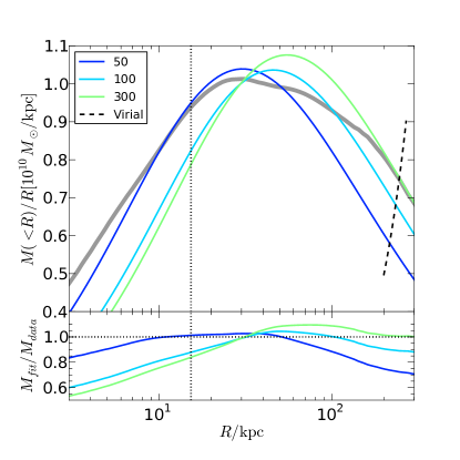
Figure 1: The mass profile (scaled as $M(<R)/R$) of halo A. In the upper panel, the grey shaded line shows the true mass profile of the dark matter distribution, while the different coloured lines show NFW profiles from maximum likelihood fits within $50,100$ and $300$ kpc respectively. The black dashed line (labelled virial) shows Eq. (11). It crosses each coloured line at the virial radius of each profile. The vertical dotted line marks the scale radius, $r_{\rm s}$. The lower panel shows the ratio of the fitted mass and the true mass as a function of the enclosing radius.

3.3 Template profiles: defining the true potential and halo parameters

To fit the halo potential using the oPDF method and assess any biases in the fit, we need to parametrize the potential with some functional form and also define the true parameters of the potential function.

One choice of parametrization is the widely used NFW profile (Navarro et al., 1996, 1997),

$$\rho(r)=\frac{\rho_{\rm s}}{(r/r_{\rm s})(1+r/r_{\rm s})^{2}},$$ (10)

where $r_{\rm s}$ is the scale radius at which $d\ln\rho/d\ln r=-2$ and $\rho_{\rm s}$ sets the density at this radius. These two parameters can be analytically related to the virial mass and concentration parameters. The virial mass is defined as the mass inside a virial radius, $R_{\rm v}$, where the enclosed density is $\Delta_{\rm v}$ times the critical density of the universe

$$M=\frac{4\pi}{3}\Delta_{\rm v}\rho_{\rm c}R_{\rm v}^{3}.$$ (11)

Throughout this paper, we adopt $\Delta_{\rm v}=200$. The concentration parameter is defined as $c=R_{\rm v}/r_{s}$. With this parametrization, one may choose to use the best-fitting parameters of the density profile as the true parameters. However, such a choice would be problematic if an NFW profile is not a good description of the halo density profile in question, in which case the best-fitting NFW parameters could depend on how the fit is performed. To demonstrate this, we fit the density profile of halo A using a maximum likelihood method. Note that dynamical modelling is not involved here, and the fit is purely to characterize the true mass distribution of the halo. The extended likelihood (Barlow, 1990), ${\cal L}$, can be written as

$$\ln{\cal L}=\sum_{i}\ln\rho(r_{i})-N_{\rm pred},$$ (12)

where $N_{\rm pred}=\int_{\rm window}\rho(r)/m_{\rm p}\,\mathrm{d}^{3}r$ is the predicted number of particles in the data window, with $m_{p}$ being the particle mass, and $\rho(r)$ the NFW density profile given by Eq. (10) with parameters $(\rho_{\rm s},r_{\rm s})$. $r_{i}$ is the radial coordinate of the $i$-th particle and the summation runs over all the particles in the data window. This method is, in the limit of infinitesimal bins, equivalent to fitting to a binned profile provided one takes account of the Poisson distribution of the counts inside each bin. We fit the dark matter distribution around halo A over several different radial ranges, with outer cuts of $50,100$ and $300$ kpc respectively. The best-fitting mass profiles along with the real mass profile are shown in Fig. 1. It is obvious that the fits differ from each other, and none of them describes well the full mass profile out to the virial radius. The inferred virial masses can differ by more than $30\%$. We note that halo A is an extreme example which deviates grossly from NFW, while the remaining four Aquarius haloes agree much better with the NFW form.

Given the poor performance of the NFW parametrization for halo A, it would be problematic to define the true halo mass, concentration or potential parameters from a best-fitting NFW profile. Put another way, any fit that adopts an NFW parametrization also suffers from systematics introduced by deviations of the real halo profile from the NFW form. To eliminate this systematic uncertainty, we will describe the potential using parametrized template profiles that are able fully to match the true profile. For each halo, we first extract the true potential profile from the spherically averaged density profile. Specifically, the potential at a given point is evaluated as

$$-\psi(r)=G\sum_{r_{i}<r}\frac{m_{i}}{r}+G\sum_{r_{i}\geq r}\frac{m_{i}}{r_{i}},$$ (13)

where $r_{i}$ and $m_{i}$ are the radial position and mass of the $i$-th particle. In practice, the profile is extracted at a sequence of radii and then interpolated at any other radius. Once a true profile is extracted, we generalize it to a two parameter family by varying its scale and amplitude. Specifically, for each real profile, $\psi(r)=f(r)$, we generate a parametric template as

$$\psi(r)=Af\left(\frac{r}{B}\right),$$ (14)

where $A$ and $B$ are dimensionless scale parameters. These two parameters can be mapped to $M$ and $c$ following the procedure in Appendix A. The true parameters ($M_{0},c_{0}$) of the halo are unambiguously defined by locating where in the true density profile the spherical overdensity matches the virial overdensity criterion and where the profile has a logarithmic slope of $-2$.

We will consider both the NFW and the template parametrizations when fitting the potential.

4 Application to DM Haloes

4.1 The dynamical state of Aquarius haloes

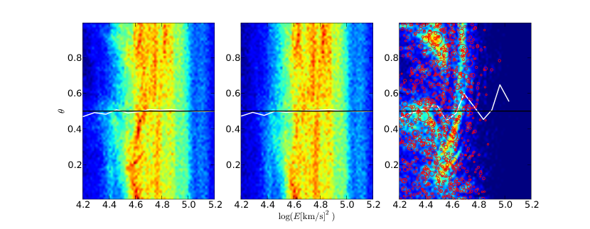
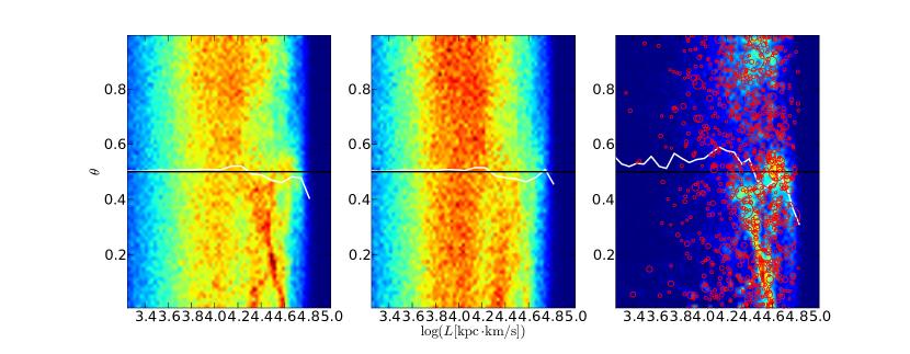
Figure 2: The phase space distribution of particles in halo A. Top and bottom panels show the distributions in $E-\theta$ and $L-\theta$ spaces respectively. The left column shows the distributions of all the particles in the sample. The middle column shows that with subhalo particles removed. The right column shows the distributions of subhalo particles alone. Each subhalo with more than 1000 particles is also marked by a red circle in the right hand panels. In all the panels, only particles with $1<r<300~{}{\rm kpc}$ are used. The white lines are the median $\theta$s. The images colour code the number of particles in each pixel. The contrast of each panel has been individually optimized.

Once the real potential is known (Eq. 13), we can examine the distribution of particles in ($\theta,E,L$) space prior to any fit. According to Eq. (3), for any system in a steady state, $\theta$ should be uniformly distributed for particles in any bin of $E$ or $L$. In Fig. 2, we show the example of halo A in such coordinates. In the left panels, all the particles within $1-300$ kpc from the halo centre are used. We are not concerned with the distributions along the $E$ and $L$ directions. Along the $\theta$ direction, overall, at fixed $E$ or $L$ the particle distributions are close to uniform. However, one can still identify clumps in phase space which perturb the uniformity. In the rightmost panels only particles from subhaloes identified by subfind (Springel et al., 2001) are plotted. The coordinates of subhaloes with more than 1000 particles are overplotted as red circles, with larger circles corresponding to more massive subhaloes. The remaining particles representing a smooth component are plotted in the middle column. Comparing the three columns, it is obvious that substructures introduce perturbations to the uniform $\theta$-space distribution of the host halo. These perturbations are twofold: first the particles inside subhaloes are locally clustered and break the uniform distribution; secondly, the potential of the subhaloes exists as perturbations to the potential of the smooth host halo, affecting the orbits of nearby particles. The existence of locally clustered structures makes the real particle distribution noisier than a Poisson realization of a smooth uniform field, and degrades the consistency between the two. In principle, substructures can be defined as locally overdense structures in phase space, and a phase space substructure finder could be designed to excise them and optimize the uniformity of the distribution of the remaining background particles. In practice, as we find subhaloes with subfind, the removal of substructures may not always increase the dynamical uniformity of the system unless the substructure finder is designed to do so.

Compared with the smooth component, subhaloes occupy relatively low binding energy and high angular momentum orbits. Despite the clumpy distribution of subhalo particles, they do not appear to bias the $\theta$ distribution significantly in any particular direction. We will come back to this point when fitting the mass and concentration of the haloes.

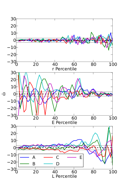
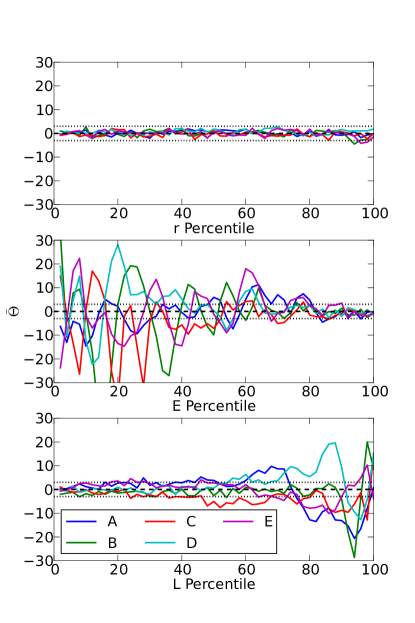
Figure 3: The normalized mean phase deviation profile of Aquarius DM haloes. From top to bottom, we bin the halo particles according to their $r,E,L$ coordinates respectively, with equal numbers of particles in each bin. The mean phase deviation, $\bar{\Theta}$, is evaluated in each bin, and plotted as a function of the percentile values in the respective coordinate. Different colour lines represent different haloes. The dashed and dotted reference lines mark the 0 and $\pm 3\sigma$ discrepancy levels. The left panels show the profiles of the full sample. The right panels show that with subhalo particles removed. See the online version for a coloured plot.

In Fig. 3, we explore deviations from a steady state of the DM tracer at different values of $r,E$ and $L$ in terms of the normalized mean phase deviation, $\bar{\Theta}$, which measures the discrepancy level from a uniform distribution. For each halo, we calculate the mean phase within bins of phase-space coordinates $r$, $E$ or $L$. We create the bins with equal numbers of particles per bin, so that they have the same statistical noise, allowing direct comparison of $\bar{\Theta}$ across the bins. The bins are labelled by the percentiles of the respective sorted phasespace coordinate, $r$, $E$ or $L$. Recall that, if the tracer is in a steady state, then in the large sample limit, $\bar{\Theta}$ is distributed like a standard normal variable.

Consistently with the physical picture displayed in Fig. 2, the DM particles have a mean phase deviation broadly consistent with zero. As seen from the left column, the discrepancy is most significant at large radius, low binding energy and high angular momentum, revealing a higher level of systematics at these locations. Note low $E$ and high $L$ regions are also where subhaloes are most abundant as seen in Fig. 2, and it is also well known that subhaloes tend to occupy the outer halo (see, e.g., Springel et al., 2008). The panels of the right hand column are the same as the left, but with subhalo particles removed from the tracer. In calculating the radial profile, the radial limits of the data window, $r_{\rm min}$ and $r_{\rm max}$, have been adjusted to the bin edges, so the radial profile examines the local uniformity of particles. After removing subhalo particles, local dynamical consistency is significantly improved at large radius. However, we see from the middle and bottom panels of Fig. 3 that this has little effect on the dynamical consistency within individual orbits over the full radial range.

Note that $\bar{\Theta}$ correlates with the depth of the proposed potential and a positive $\bar{\Theta}$ indicates the current potential is deeper than a best-fitting potential (Paper I). As seen in Fig. 3, at large $r$, $L$ and low $E$, the mean phase deviation can be significantly higher than one would expect from a uniform distribution, which would lead to a level of systematic uncertainty significantly larger than the statistical noise in the best-fitting potential. However, overall the fluctuation is still stochastic with no preferred sign. This indicates that if one is going to fit the potential, then deviations from our model assumptions are unlikely to bias the model parameters in a particular direction; instead, the biases would fluctuate stochastically. Despite this, these biases are still systematic rather than statistical in nature, as they are tied to the model assumptions, not to the sample size. In the following section, we aim to quantify the level of such systematic uncertainty in the best-fitting parameters of the halo potential.

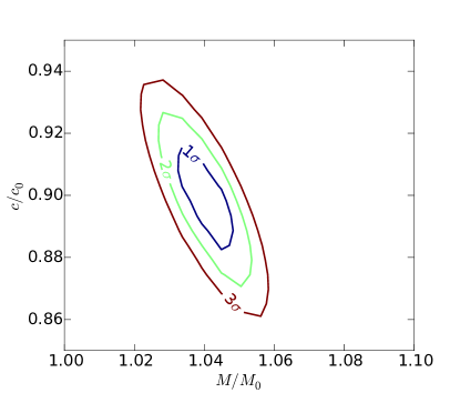
Figure 4: The 1, 2 and 3$\sigma$ confidence contours for the full sample of halo A fitted with the oPDF likelihood using the template profile. The parameters are in units of their true values.

4.2 Fitting the halo potential with DM as tracers

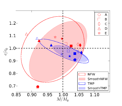
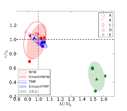
Figure 5: Left: fitted parameters of Aquarius haloes using the radial likelihood estimator. Different shaped symbols denote different haloes. The red and blue colours denote the fitting results using NFW and template profiles (labelled TMP) respectively. In both cases, the open symbols show the fits with the full samples, while the filled ones show those for the smooth samples, i.e., with subhalo particles excluded. For each combination of sample and profile, we combine the five haloes to estimate a mean and a covariance matrix for the parameters, and plot the $1\sigma$ contour (the ellipses, open or filled) in the same style for a bivariate Gaussian with the estimated mean and covariance. Right: same as the left, but also showing the fits from Wang et al. (2015) to the smooth DM sample using a $f(E,L)=L^{-2\beta}F(E)$ model (green symbols and ellipse). See the online version for a coloured plot.

With the potential functions and their true parameters defined in Section 3.3, we can proceed to fit the potential profiles with our oPDF method, and quantify the level of systematic uncertainty in the fitted parameters. We adopt the binned radial likelihood estimator, with 50 logarithmic bins. Fitting with a different number of radial bins gives consistent results. For both NFW and template parametrizations, we fit two datasets: 1) all the dark matter particles inside $1-300$ kpc, i.e, the full sample; 2) the former but with all the subhalo particles removed, i.e, the smooth sample. Because we aim to quantify the systematic uncertainties due to deviations from model assumptions, we need to make sure that the statistical noise, which is determined by sample size, is small enough. As an example, in Fig. 4 we show the statistical confidence contours of halo A from the template fit. These error estimates are consistent with the scatter among independent subsamples of the parent halo. The $1\sigma$ error is around $0.005$ dex for our sample of $10^{6}$ particles, quite consistent with our expected scaling of $0.1/\sqrt{N/1000}$ dex. Such an accuracy should be sufficient for detection of systematic biases larger than $1\%$.

The best-fitting parameters in units of the true parameters are plotted in the left panel of Fig. 5. Overall, the fitted $(M,c)$ parameters largely agree with their true values, with a bias generally smaller than $10\%$. The typical bias quantified by the scatter among the five haloes is $\sim 5\%$ as listed in Table 3. For each parametrization and dataset, we combine the five haloes to estimate a mean and a covariance matrix for the parameters, and plot the one-sigma contour for a bivariate Gaussian with the estimated mean and covariance. Note these contours are an estimate of the systematic uncertainties, since the statistical noise of the model is negligible given the sample sizes. Consistently with our expectation from the mean phase profiles, there is not a definitive systematic bias but rather, as far as we can tell from the small sample of haloes, the scatter is mostly stochastic from halo to halo.

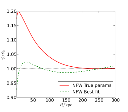
Figure 6: The potential profile of halo A and its NFW parametrization. We plot the ratio between the parametrized NFW potential, $\psi$, and the true potential, $\psi_{0}$, of the halo as a function of radius. For the dynamical modelling only the potential difference is relevant and so the zero-points of the NFW potentials have been adjusted to produce the true potential value at the virial radius. The red solid line corresponds to the NFW potential profile using the true parameters and the green dashed line to the NFW parameters found from the oPDF likelihood estimated from all the dark matter particles.

Comparing the fits with and without subhalo particles, there is not a significant improvement in the latter. When NFW profiles are adopted in the fits, the accuracy is comparable to that achieved with template profiles in most cases. This reflects the fact that most haloes are well described by NFW profiles. Note that the significantly larger confidence regions in NFW fits as marked by the ellipses in Fig. 5 is caused purely by halo A, whose dynamical fit shows a bias in concentration up to 30%. This is due to the fact that the density profile of halo A differs significantly from NFW, as is evident from Fig. 1. In Fig. 6 we show the disagreement in halo A from a different perspective, by comparing the NFW parametrization of the halo potential with the true potential. When the set of true halo parameters are used, the NFW potential is consistently overestimated inside the halo. The dynamical fit adjusts the parameters so that the NFW potential agrees with the true potential to within 5 percent for most of the radial range. The best-fit NFW potential agrees better with the true potential, reflecting the fact that the dynamical fit largely recovers the true potential by force-fitting the NFW parametrization, despite giving different parameters from the true values. It is quite interesting to see that when the template profile is adopted, halo A does not appear to be more biased than the other haloes, meaning that a deviation from the NFW form does not necessarily mean a lack of equilibrium.

In the right panel of Fig. 5, we compare our fits to those obtained from a conventional DF method that describes the phase space density only as a function of $(E,L)$ of the particles (Wang et al., 2015). Specifically, the phase space probability is assumed to have the form $\mathrm{d}P(\vec{r},\vec{v})=f(E)L^{-2\beta}\,\mathrm{d}^{3}r\,\mathrm{d}^{3}v$, where $\beta$ is a parameter describing the velocity anisotropy, with $f(E)$ further determined by inverting a double-powerlaw tracer density profile inside an NFW potential (see Eq. 12 in Wang et al., 2015 for further details). This distribution function describes a family of models with constant anisotropies, while in general more flexible models can be constructed (e.g. Wojtak et al., 2008; Posti et al., 2015; Williams & Evans, 2015b). In contrast to the fairly unbiased fits with our method, this $f(E,L)$ method suffers from a $\sim 50\%$ net bias in the parameters. As discussed in Wang et al. (2015), this can be attributed to the fact that the $f(E,L)$ DF only describes gravitationally bound systems by construction (see also section 6.3.1 of Paper I), and struggles to match the distribution of the loosely bound particles. Because our oPDF method has no prerequisite on the distribution of orbits (hence no prerequisite on the energy distribution), our fits show no such net bias. On the other hand, the $f(E,L)$ fits exhibit a comparable amount of halo to halo scatter in the parameters to ours, reflecting that our method does capture the minimum irreducible uncertainty associated with steady-state models.

5 Application to mock stellar haloes

Table 1: Basic properties of the stellar haloes, within $10-300$ kpc. $N_{\rm tot}$ is the total number of star particles, $N_{\rm smth}/N_{\rm tot}$ is the fraction of particles in the smooth component and $m_{\rm smth}/m_{\rm tot}$ is the mass fraction of particles in the smooth component.

Halo	$N_{\rm tot}$	$N_{\rm smth}/N_{\rm tot}$	$m_{\rm smth}/m_{\rm tot}$	$D$
A	$5.4\times 10^{5}$	0.50	0.34	9.6
B	$7.4\times 10^{5}$	0.72	0.36	9.6
C	$5.3\times 10^{5}$	0.70	0.43	5.9
D	$8.1\times 10^{5}$	0.60	0.52	5.5
E	$5.1\times 10^{5}$	0.47	0.18	9.5

In Fig. 7 we show the phase space distribution of stars in halo A. Unlike the DM tracer which is only slightly perturbed by subhaloes, the halo stars are dominated by those in the satellite subhaloes. The mass fraction contained in satellite galaxies is $50\%-70\%$ (Table 1) in the radial range of interest. These satellite stars are obviously not in equilibrium with the rest, and can be observationally identified and removed as satellite galaxies. In what follows, we will only use the “smooth” component of halo stars, i.e, those excluding satellite stars, as our tracer sample. In total, each halo has $(2-5)\times 10^{5}$ smooth star particles within $10-300$ kpc, yielding a statistical uncertainty of $\sim 2\%$ in mass and concentration.

The mean phase deviation profile is shown in Fig. 8. As for the profile of DM tracers, overall $\bar{\Theta}$ is consistent with zero, with the highest scatter seen at large radius, low binding energy and high angular momentum. Note that stars with low binding energies are also those that have been accreted recently (Wang et al., 2015). The scatter in the star profiles also appears higher than that in the DM case.

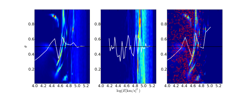
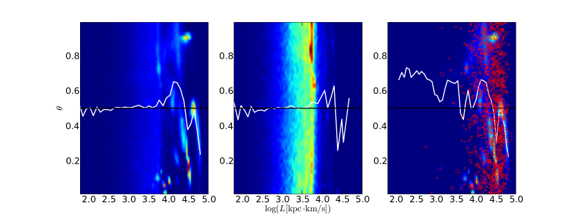
Figure 7: As Fig. 2 but for the stars in the level 2 halo A. From left to right the distributions of all the stars, the “smooth” component (all stars excluding satellites), and those in satellite subhaloes. The contrast of each panel is individually optimized.

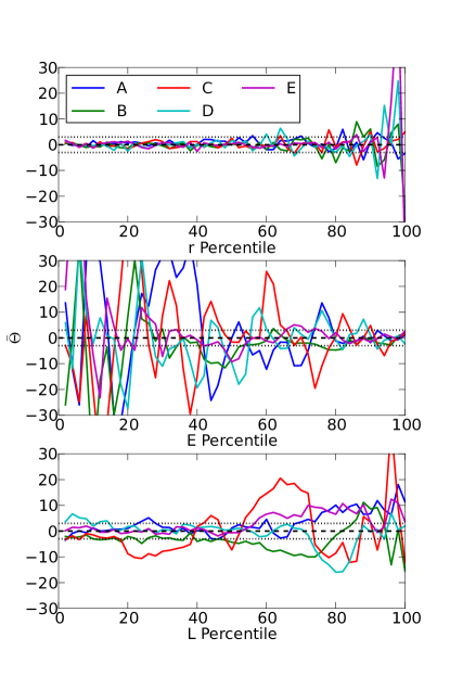
Figure 8: The mean phase deviation profile of Aquarius stellar haloes. This is the same as the right hand side of Fig. 3, but for star particles. From top to bottom, we bin the star particles according to their $r,E$ and $L$ coordinates respectively, with equal numbers of particles in each bin. The mean phase deviation, $\bar{\Theta}$, is evaluated in each bin, and plotted as a function of the percentile values in the respective coordinate. Different coloured lines represent different haloes as indicated in the legend. The dashed and dotted reference lines mark the 0 and $\pm 3\sigma$ discrepancy levels. Only the smooth component of the halo stars is used. See the online version for a coloured plot.

The fits using stars are plotted in Fig. 9 for both the template and NFW profile models. For individual haloes, the deviation from the true parameters can be as high as 40%. For comparison, the fits and $1\sigma$ contours from the $f(E,L)$ method of Wang et al. (2015) and those from the DM tracers in the previous section are also plotted.

Overall, we do not observe a statistically significant net bias in the fits with the current sample of five haloes, even though the $f(E,L)$ method applied to stars is only marginally unbiased at the $1\sigma$ level. In other words, the systematic bias varies from halo to halo in a stochastic way. Despite this stochastic behaviour, we have checked that the systematic bias does not change with sample size, so it is indeed a systematic rather than a statistical error. There is a negative correlation between the mass and concentration parameters in the template fits, which is similar to the correlation in the statistical noise of the two parameters. This correlation is absent in the NFW fits only because halo A is not well described by NFW and this biases the fit significantly. A viable explanation of this behaviour of the systematic bias lies in the deviation of the tracer population from a steady state. For example, the existence of correlated phase angles in streams and caustics implies that different tracer particles are not independent. As a result, the constraining power of a set of particles in a stream is less than that of an equal number of independent particles. In the large sample limit, when each stream is sufficiently sampled, the errors on the inferred model parameters do not vanish but are limited by the effective number of independent streams or particle clumps. This is an intrinsic property of each halo. Hence it is understandable that we are left with irreducible stochastic biases in well sampled haloes. In addition, these residual errors are expected to exhibit similar parameter correlations to the statistical noise. Note that while the DM fits exhibit only $\sim 5\%$ scatter, the scatter for the stellar fits is typically $\sim 20\%$.

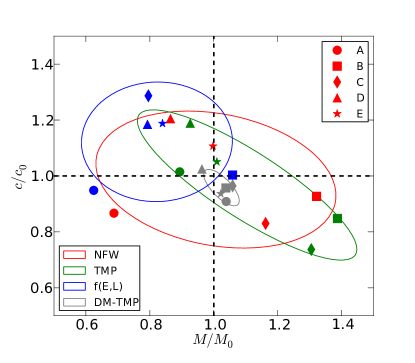
Figure 9: As Fig. 5, but showing the results of the dynamical fits to the halo stars. As indicated in the legends, symbols of different shapes represent different haloes, while different colours distinguish different datasets and model profiles. Red and green show fits to stars adopting NFW and template profiles respectively; blue shows the fit from Wang et al. (2015) to stars combining radial and tangential velocities using a specific $f(E,L)$ model; grey shows the template fit applied to the smooth DM tracer. The symbols are the results of fits to individual haloes, while the large ellipses mark the estimated $1$-$\sigma$ confidence regions for each type (i.e., combination of dataset and model) of fit estimated from the sample of five haloes. See the online version for a coloured plot.

Since stars and DM tracers have different $E$-$L$ distributions, they occupy a statistically different set of orbits. This implies the tracers potentially have different spatial distributions. As a result, they could be sampling different parts of the halo, or the same region but with different weights given to the local deviations of the halo potential. It is possible that the different sampling has resulted in the stars yielding a large scatter in the inferred halo properties. To see whether this is the case, we select dark matter particles that have the same $E$-$L$ distribution as the stars to create a star-like dark matter sample. Subhalo particles are removed from the DM and star samples before sampling the $E$-$L$ distribution and the radial coordinates are ignored when constructing the samples. The same fitting procedure is then applied to this star-like dark matter sample. The results are shown in Fig. 10. By drawing a sample with the stellar $P(E,L)$ from DM particles, the scatter in the fits is actually slightly decreased (probably due to the removal of the less virialized outer halo particles) compared to the DM fits, and is much smaller than that in the star fits. This shows that the tagged stars are indeed in less of a steady state than the dark matter.

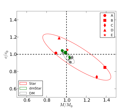
Figure 10: Comparison between the results of stellar and the DM dynamical fits. The “Star” and “DM” fits are the same as in Fig. 9, using stars and DM particles respectively. The “dmStar” fit uses a sample of DM particles selected to have the same $E$-$L$ distribution as that of the stars. Subhalo particles have been removed in all three cases and only the template profiles are used. See the online version for a coloured plot.

We remark that even though for the star samples the scatter in Fig. 8 is higher at large radii, low binding energies and high angular momentum, we do not detect a systematic decrease in the biases of the fitted parameters as we exclude the large radii, low energy or low angular momentum regions. The lack of systematic improvements in bias when excluding the regions with large scatter is consistent with our previous argument that the biases are limited by the effective number of independent streams. Also note the bias and scatter are separate quantities, and we have observed that in the high scatter regions the mean profile does not appear more biased.

6 Half mass constraint

In Paper I we used Monte-Carlo samples to demonstrate that the mass profiles are best constrained near the median radius of the tracer population. Similar best-constrained masses also exist in several previous studies using very different methodologies (Walker et al., 2009; Wolf et al., 2010; Amorisco & Evans, 2011, see section 5.1 of Paper I for more discussion). Here we revisit this discovery with the Aquarius haloes. In Fig. 11 we plot the constrained mass profile from the DM and star tracers in halo A. Note our likelihood method constrains not only the characteristic mass, but also the shape of the mass profile. If the profile shape is biased then the bias in enclosed mass varies with radius. Consistent with our previous findings, the mass is best constrained near the half-mass radius of the tracer. Comparing these best-constrained masses, the bias in stars is still significantly larger than that in DM. This is also consistent with our test using a star-like DM tracer in Fig. 10, where we find that the different samplings of the star and DM tracers are not the cause of the different bias levels. For comparison, the best-fitting profile of the star-like DM tracer is also plotted, and shows a bias comparable to the original DM fit. As listed in Table 2, stars yield an average bias of $\sim 5\%$ at $r_{1/2}$ when using the template fits, while the DM yields only $\sim 1\%$. The star-like DM tracers have $r_{1/2}$ close to that of the stars, but gives almost no bias at $r_{1/2}$. As far as the constraints at $r_{1/2}$ are concerned, fitting with NFW profiles gives quite similar results to template fits, indicating that the half mass constraint is less sensitive to the adopted functional form for the halo density profile (see also Paper I). However, models with extra assumptions could still lead to significant bias at $r_{1/2}$. For example, fitting the DM tracers with the $f(E,L)$ method in Wang et al. (2015) produces an average mass bias of $13\%$ at $r_{1/2}$ (Table 3).

Table 2: Tracer half-mass radius $r_{1/2}$ and mass bias $b_{1/2}$ at $r_{1/2}$, from fits to the smooth component of DM, star, and “dmStar“ tracers. “dmStar” refers to DM tracers selected to have the same $E$-$L$ distribution as the stars, as in Fig. 10. We list the biases from template fits by default. For DM and star tracers, biases from NFW fits are also given in parenthesis.

Halo	DM $r_{1/2}/$kpc	DM $b_{1/2}$	Star $r_{1/2}/$kpc	Star $b_{1/2}$	dmStar $r_{1/2}$	dmStar $b_{1/2}$
A2	103	0.00 (0.05)	41.7	-0.07 (-0.02)	41.6	-0.01
B2	85.4	0.01 (0.03)	18.8	0.05 (0.05)	19.0	0.01
C2	86.2	0.03 (0.05)	48.2	0.03 (0.04)	47.4	0.00
D2	103.1	-0.02 (0.00)	32.8	0.04 (0.05)	33.1	0.00
E2	90.1	-0.00 (0.00)	18.6	0.04 (0.02)	18.6	0.00

We emphasize that since we are not only interested in the mass constraint at a single radius but also in the full profile, any parametrization of a specific density profile should be equivalent. As long as the constraints are fully described in terms of the parameter covariance or the 2-dimensional confidence contour, the constraints on the full profile can always be recovered and translated to constraints in any other parametrization of the profile. Our parametrization is intentionally chosen to constrain the most popular parameters, the virial mass and concentration of haloes.

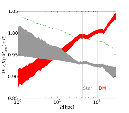
Figure 11: The template-fitted mass profile of halo A, using smooth DM (red) and smooth star (grey) particles as tracers respectively. The shaded regions are the $1$-$\sigma$ constraints on the mass profile, normalized by the true profile. The vertical lines mark the half-mass radius of the two tracers. The green dotted line is the best-fitting profile from the star-like DM tracer (i.e., “dmStar” in Fig. 10).

7 Summary and conclusions

Table 3: Summary of the different fits to the halo density profile. For each combination of data and method, we list the fitted parameters averaged over the five haloes ($\bar{x}$) and their halo-to-halo standard deviation ($\sigma$) in the form $\bar{x}\pm\sigma$. The mass ($M$) and concentration ($c$) parameters are normalized by their true values, $M_{0}$ and $c_{0}$. The mass bias at the tracer half-mass radius, $b_{1/2}$, is also listed in the same form. Different columns refer to different combinations of data and methods. “DM-Full”, “DM” and “Star” refer to full DM, the smooth DM (DM-Full excluding subhalo particles), and smooth star tracers. “dmStar” refers to DM samples selected to have the same $E$-$L$ distribution as stars. “NFW” and “TMP” refer to fits using NFW or template potential profiles. $f(E,L)$ refers to the $(r,v_{r},v_{t})$ fit in Wang et al. (2015) using an $f(E,L)$ distribution function.

	DM:NFW	DM:TMP	DM-Full:TMP	DM:$f(E,L)$	Star:NFW	Star:TMP	Star:$f(E,L)$	dmStar:TMP
$M/M_{0}$	$0.97\pm 0.07$	$1.00\pm 0.05$	$1.02\pm 0.04$	$1.54\pm 0.05$	$1.00\pm 0.25$	$1.10\pm 0.23$	$0.82\pm 0.16$	$0.99\pm 0.03$
$c/c_{0}$	$0.99\pm 0.17$	$0.98\pm 0.06$	$0.96\pm 0.04$	$0.48\pm 0.13$	$0.99\pm 0.16$	$0.97\pm 0.18$	$1.12\pm 0.14$	$1.01\pm 0.03$
$b_{1/2}$	$0.02\pm 0.02$	$0.00\pm 0.01$	$-0.01\pm 0.02$	$0.13\pm 0.02$	$0.03\pm 0.02$	$0.02\pm 0.04$	$-0.02\pm 0.01$	$0.00\pm 0.01$

We have applied our oPDF estimator to tracers in five simulated haloes from the Aquarius project, to study the level of systematic biases in fitting the mass distribution of Milky-Way sized haloes. We focus on effects from the parametrization of the halo potential, the existence of subhaloes, and the types of tracer used. Assuming a spherical symmetric potential, our method only makes use of the dynamical equilibrium of the tracer. As a result, the level of systematic biases detected in our analysis can, in general, be interpreted as the minimum level of bias present in any time-independent DF modelling of dynamical tracers that assumes a spherical potential. With our sample of five haloes, we do not have a reliable detection of a common bias in our method towards any particular direction in parameter space. Instead, we focus on characterizing the average amplitude of the bias in each fit. We quantify this as the rms scatter of the biases for individual haloes, and summarize them in Table 3. The method works very well on DM tracers, with a level of systematic bias at only $\sim 5\%$. Assuming an NFW profile does not significantly affect the fits in most cases, except in one case out of five where the density profile of the halo (Aq-A) differs significantly from the NFW form, leading to a much larger bias ($\sim 30\%$) when adopting the NFW profile. However, the deviation from the NFW profile in halo A does not affect the equilibrium of the DM tracer. Subhaloes exist as perturbations that give rise to deviations from steady state for the tracers, but only affect the dynamical fits using DM tracers by $\sim 1\%$. In contrast to the fairly good fits to the DM tracers with our method, a conventional DF fit adopting a specific $f(E,L)$ DF (Wang et al., 2015) yields a net bias of $50\%$ in mass and concentration on average. This is caused by the additional assumptions made in the $f(E,L)$ DF that restricts the allowed distribution of orbits. On the other hand, the halo-to-halo variation in the bias is comparable to that in our method, demonstrating that our method gives the minimum uncertainty in mass modelling assuming time-independent DFs.

Applying our method to mock stars results in a higher level of bias, $b\sim 20\%$, comparable to that in the $f(E,L)$ DF method tested in Wang et al. (2015) which, however, also suffers from a non-zero net bias. The larger bias using star tracers is not due to different phase-space sampling by stars compared to DM particles: DM tracers constrained to sample the phase space $E$-$L$ distribution in the same way as the stars yield biases at the same level as the original DM tracers. The larger deviation of tagged stars from a steady state is not surprising because they involve the 1% most-bound particles of their host subhalo at the time of star formation. By definition, these particles are the most resistant to tidal stripping and subsequent mixing. Even though we only use the stripped population of tagged particles, they are still farther from equilibrium than the smooth component of the host halo.

It is well known that dynamical tracers best-constrain the host mass near the tracer’s half-mass radius, $r_{1/2}$ (Walker et al., 2009; Wolf et al., 2010; Amorisco & Evans, 2011). Although we adopt a vastly different method from those analysis, a similar behaviour is also observed in our analysis. Near $r_{1/2}$, the mass biases, $b_{1/2}$, are much reduced, and also become less sensitive to the functional form of the halo profile assumed in our model. Larger biases are still observed for stars, $b_{1/2}\sim 5\%$, compared with $b_{1/2}\sim 2\%$ for DM tracers. The $f(E,L)$ method that poorly fits the DM tracer produces a much larger bias, $b_{1/2}\sim 10\%$. Although the bias at $r_{1/2}$ is significantly smaller than the bias for the total mass, in reality $b_{1/2}$ together with the constraint on the profile shape at $r_{1/2}$ is equivalent to the joint constraint in the mass-concentration space. Given the full mass-concentration covariance matrix, one can readily obtain the mass constraint at any radius including $r_{1/2}$. While $r_{1/2}$ depends on the tracer, $M$ and $c$ are intrinsic properties of the halo.

In this work we frequently compare our results with those of Wang et al. (2015) who used a specific model of the $f(E,L)$ family to study the same haloes. We demonstrate that the extra assumptions in that model beyond time-independence and spherical symmetry have resulted in a worse performance compared with the oPDF. There are more flexible distribution functions that can improve over the one assumed in Wang et al. (2015), for example, by allowing for varying anisotropies (e.g. Wojtak et al., 2008; Williams & Evans, 2015b). More generally, there may exist a true model that describes well the distribution function of the tracers. However, such a true model has to be known a priori to fit the tracers correctly, which is a highly challenging task if at all possible. At the same time, any specifically proposed distribution function has generally has limitations stemming from extra assumptions over and above the Jeans theorem. These extra assumptions may not be obeyed by an arbitrary tracer sample. As such, the results obtained using the oPDF method which makes minimal assumptions are particularly robust, and the comparison with the specific model of Wang et al. (2015) therefore serves to illustrate the limitations of restricted models. In particular, since the statistical noise has been controlled to be negligible in our analysis, the level of systematic bias detected with the oPDF is the minimum level of systematic bias expected from any model that assumes a spherically symmetric and time-independent distribution function.

Note that the stars used in this work are generated from a particle tagging method that is a relatively simple way of approximating the phase-space distribution of stars. Several factors, including insufficient mass resolution (the weighting and multiple tagging of star particles), the time discreteness of the tagging (the method works with snapshots), and the lack of dissipation and back-reaction on the potential from stars, could all potentially affect the degree of realism with which the tagged stars represent the dynamics of real stars. Due to these limitations, the results from the tagged stars should only be taken as indicative. Also note that only five haloes are studied in this work and these may not be very representative of our Milky Way halo. In a follow up work, we will apply the method to a larger sample of haloes modelled using SPH simulations of the Local Group for a more realistic assessment of the dynamical state of tracers in Galactic haloes.

Appendix A Parameters of template profiles

To connect template parameters $A$ and $B$ in Eq. (14) to physical parameters, we can define

$$A =\psi_{\rm s}/\psi_{\rm s0},$$ (15)

$$B =r_{\rm s}/r_{\rm s0},$$ (16)

where $r_{\rm s}$ is a scale radius at which the profile has some predefined shape, and $\psi_{\rm s}$ is the potential at $r=0$. We choose $r_{\rm s}$ to be the radius where $d\ln\rho/d\ln r=-2$, to be consistent with an NFW parametrization. $r_{\rm s0}$ and $\psi_{\rm s0}$ are the corresponding quantities of the true profile. Hence this template profile is parametrized by $(A,B)$ or equivalently by $(\psi_{\rm s},r_{\rm s})$. We can also define equivalent mass and concentration parameters. For each profile, the virial mass, $M$, and virial radius, $R_{\rm v}$, can be defined following the same spherical-overdensity definition as in Eq. (11), and the concentration can be defined through $c=R_{\rm v}/r_{\rm s}$, consistently with NFW. The mass and concentration parameters of the true profile (i.e., the template with $A=1,B=1$), $M_{0}$ and $c_{0}$, are by definition the true parameters of the halo, and can be obtained unambiguously from the true profile without fitting. If the halo is perfectly NFW, then the true parameters defined this way are also the best-fitting NFW parameters to the density profile. When the density profile differs from NFW form, however, the true parameters, $M_{0}$ and $c_{0}$, should be interpreted as the spherical overdensity mass and the contrast of the spherical overdensity radius, $R_{\rm v}$, to the slope $-2$ radius, $r_{\rm s}$, rather than being any best-fitting NFW parameters.

With the template parametrization, the inversion from any set of ($M,c$) parameters back to ($A,B$) is also straight-forward. Note that the mass profile of the template scales as

$$M(r) =\frac{\psi^{\prime}(r)r^{2}}{G}$$ (17)

$$=ABm\left(\frac{r}{B}\right),$$

where $M(r)$ is the mass profile of the template with parameters ($A,B$), $\psi^{\prime}(r)$ is the derivative of the template potential, and $m(r)$ is the true mass profile. Hence $M=ABm(R_{\rm v}/B)$. After obtaining ($R_{\rm v},r_{\rm s}$) from ($M,c$), one can solve ($A,B$) as follows

$$B =\frac{r_{\rm s}}{r_{\rm s0}}$$ (18)

$$A =\frac{M}{Bm(R_{\rm v}/B)}.$$ (19)

To create the templates numerically, we extract both the potential profiles and the cumulative density profiles $\rho(<r)\propto{\psi^{\prime}(r)}/{r}$ from the particle distribution of each halo. The $\rho(<r)$ is provided to avoid the need for numerical differentiation of the potential profile.

References

- Amorisco & Evans (2011) Amorisco N. C., Evans N. W., 2011, MNRAS, 411, 2118, arXiv:1009.1813
- Barlow (1990) Barlow R. J., 1990, Nucl.Instrum.Meth., A297, 496
- Beloborodov & Levin (2004) Beloborodov A. M., Levin Y., 2004, ApJ, 613, 224, astro-ph/0405533
- Bower et al. (2006) Bower R. G., Benson A. J., Malbon R., Helly J. C., Frenk C. S., Baugh C. M., Cole S., Lacey C. G., 2006, MNRAS, 370, 645, astro-ph/0511338
- Cautun et al. (2014) Cautun M., Frenk C. S., van de Weygaert R., Hellwing W. A., Jones B. J. T., 2014, MNRAS, 445, 2049, arXiv:1405.7697
- Cole et al. (1994) Cole S., Aragon-Salamanca A., Frenk C. S., Navarro J. F., Zepf S. E., 1994, MNRAS, 271, 781, astro-ph/9402001
- Cole et al. (2000) Cole S., Lacey C. G., Baugh C. M., Frenk C. S., 2000, MNRAS, 319, 168, astro-ph/0007281
- Cooper et al. (2010) Cooper A. P. et al., 2010, MNRAS, 406, 744, arXiv:0910.3211
- Cooper et al. (2013) Cooper A. P., D’Souza R., Kauffmann G., Wang J., Boylan-Kolchin M., Guo Q., Frenk C. S., White S. D. M., 2013, MNRAS, 434, 3348, arXiv:1303.6283
- Frenk et al. (1988) Frenk C. S., White S. D. M., Davis M., Efstathiou G., 1988, ApJ, 327, 507
- Gibbons et al. (2014) Gibbons S. L. J., Belokurov V., Evans N. W., 2014, MNRAS, 445, 3788, arXiv:1406.2243
- Gnedin et al. (2010) Gnedin O. Y., Brown W. R., Geller M. J., Kenyon S. J., 2010, ApJ, 720, L108, arXiv:1005.2619
- Han et al. (2015) Han J., Wang W., Cole S., Frenk C. S., 2015, ArXiv e-prints, arXiv:1507.00769
- Jing & Suto (2002) Jing Y. P., Suto Y., 2002, ApJ, 574, 538, astro-ph/0202064
- Kennedy et al. (2014) Kennedy R., Frenk C., Cole S., Benson A., 2014, MNRAS, 442, 2487, arXiv:1310.7739
- Le Bret et al. (2015) Le Bret T., Pontzen A., Cooper A. P., Frenk C., Zolotov A., Brooks A. M., Governato F., Parry O. H., 2015, ArXiv e-prints, arXiv:1502.06371
- Navarro et al. (1996) Navarro J. F., Frenk C. S., White S. D. M., 1996, ApJ, 462, 563, arXiv:astro-ph/9508025
- Navarro et al. (1997) Navarro J. F., Frenk C. S., White S. D. M., 1997, ApJ, 490, 493, arXiv:astro-ph/9611107
- Navarro et al. (2010) Navarro J. F. et al., 2010, MNRAS, 402, 21, arXiv:0810.1522
- Perryman et al. (2001) Perryman M. A. C. et al., 2001, A&A, 369, 339, astro-ph/0101235
- Posti et al. (2015) Posti L., Binney J., Nipoti C., Ciotti L., 2015, MNRAS, 447, 3060, arXiv:1411.7897
- Springel et al. (2008) Springel V. et al., 2008, MNRAS, 391, 1685, arXiv:0809.0898
- Springel et al. (2001) Springel V., White S. D. M., Tormen G., Kauffmann G., 2001, MNRAS, 328, 726, astro-ph/0012055
- Walker et al. (2009) Walker M. G., Mateo M., Olszewski E. W., Peñarrubia J., Wyn Evans N., Gilmore G., 2009, ApJ, 704, 1274, arXiv:0906.0341
- Wang et al. (2012) Wang J., Frenk C. S., Navarro J. F., Gao L., Sawala T., 2012, MNRAS, 424, 2715, arXiv:1203.4097
- Wang et al. (2015) Wang W., Han J., Cooper A., Cole S., Frenk C., Cai Y., Lowing B., 2015, ArXiv e-prints, arXiv:1502.03477
- Wilkinson & Evans (1999) Wilkinson M. I., Evans N. W., 1999, MNRAS, 310, 645, astro-ph/9906197
- Williams & Evans (2015a) Williams A. A., Evans N. W., 2015a, ArXiv e-prints, arXiv:1508.02584
- Williams & Evans (2015b) Williams A. A., Evans N. W., 2015b, MNRAS, 448, 1360, arXiv:1412.4640
- Wojtak et al. (2008) Wojtak R., Łokas E. L., Mamon G. A., Gottlöber S., Klypin A., Hoffman Y., 2008, MNRAS, 388, 815, arXiv:0802.0429
- Wolf et al. (2010) Wolf J., Martinez G. D., Bullock J. S., Kaplinghat M., Geha M., Muñoz R. R., Simon J. D., Avedo F. F., 2010, MNRAS, 406, 1220, arXiv:0908.2995
- Xue et al. (2008) Xue X. X. et al., 2008, ApJ, 684, 1143, arXiv:0801.1232