The orbital PDF: general inference of the gravitational potential from steady-state tracers

Abstract

We develop two general methods to infer the gravitational potential of a system using steady-state tracers, i.e., tracers with a time-independent phase-space distribution. Combined with the phase-space continuity equation, the time independence implies a universal Orbital Probability Density Function (oPDF) $\mathrm{d}P(\lambda|{\rm orbit})\propto\mathrm{d}t$, where $\lambda$ is the coordinate of the particle along the orbit. The oPDF is equivalent to Jeans theorem, and is the key physical ingredient behind most dynamical modelling of steady-state tracers. In the case of a spherical potential, we develop a likelihood estimator that fits analytical potentials to the system, and a non-parametric method (“phase-mark”) that reconstructs the potential profile, both assuming only the oPDF. The methods involve no extra assumptions about the tracer distribution function and can be applied to tracers with any arbitrary distribution of orbits, with possible extension to non-spherical potentials. The methods are tested on Monte Carlo samples of steady-state tracers in dark matter haloes to show that they are unbiased as well as efficient. A fully documented C/Python code implementing our method is freely available at a GitHub repository linked from http://icc.dur.ac.uk/data/#oPDF.

1 Introduction

Since dark matter does not emit or absorb electromagnetic radiation, gravitational modelling is of fundamental importance to the determination of the dark matter distribution. Such modelling can be performed using either gravitational lensing (e.g., Bartelmann, 2010; Han et al., 2014), or the dynamics of tracers (e.g., stars or galaxies; see Courteau et al., 2014 for a recent review on galaxy mass inferences).

One straightforward way to perform dynamical modelling is to fit a proposed phase-space distribution function (DF) to the observed positions and velocities of tracer particles. Thanks to Jeans theorem (see e.g. Binney & Tremaine, 2008), which states that functions of the integrals of motion, $J$, are solutions of the Boltzmann equation, one can simply consider DFs of the form $f(J)$. Under certain conditions, one can invert the observed density profile, $\rho=\int f(J)\mathrm{d}^{3}v$, of the tracer to construct a specific family of $f(J)$ (e.g., Eddington, 1916; Osipkov, 1979; Merritt, 1985; Cuddeford, 1991; hereafter referred to as density profile inversion). The density profile inversion depends on the potential of the halo, and the resulting $f$ is thus potential dependent. However, some further assumptions about the functional form of $f(J)$ are required to perform the inversion. These assumptions are typically motivated either empirically (e.g., Wojtak et al., 2008; Williams & Evans, 2015a), or by mathematical simplicity (e.g., Evans & An, 2006). When proposing the DFs, one is free to choose the integrals of motion, to be either classical integrals such as energy and angular momentum, or the more theoretically appealing actions (see e.g., Posti et al., 2015; Williams & Evans, 2015b, for such recent models on halo stars).

In Wilkinson & Evans (1999) and Wang et al. (2015), solutions of the form $f(E,L)=f(E)L^{-2\beta}$ were used to constrain the potential of the Galactic halo, where $E$ and $L$ are the energy and angular momentum of tracer particles. In particular, Wang et al. (2015) applied the $f(E,L)$ method to mock stellar haloes (Cooper et al., 2010) constructed from the Aquarius simulations of $\Lambda$CDM galactic haloes (Springel et al., 2008) and found significant biases in the fitted masses. These biases suggest that the proposed $f(E,L)$ DF does not describe well the observed phase-space distribution of the mock stars. However, it is not clear whether the discrepancy is due to departures from dynamical equilibrium by the stars within the halo potential, or to the lack of generality in the proposed $f(E,L)$ functional form used to describe the distribution (e.g., Binney & Mamon, 1982). In the former case, the stars would represent an intrinsically biased tracer, and the modelling of their distribution would not give the correct potential. In the latter case, one can still hope to find a DF that fits the observed distribution with the correct potential once the extra assumptions in the functional form of $f(E,L)$ are relaxed or removed.

A method requiring no assumptions on the form of $f(E,L)$ is achievable, which is what we develop in this work. The starting point of our method is the definition of tracer. We define a tracer as a population of objects whose phase-space DF does not evolve with time (i.e., is in a steady state), so that modelling their DF at an arbitrary time is generally possible and useful. It immediately follows from this definition that the probability of observing a particle at a position on its orbit is proportional to the time it spends near that position, i.e., $\mathrm{d}P|{\rm orbit}\propto\mathrm{d}t$. Formally, this can be shown to be a result of phase-space continuity (Section 2.2). We give a thorough description on this Orbital Probability Density Function (oPDF) in Section 2, with further discussion in Section 6.1.

This simple relation actually contains all the information required to model the potential of the system. We demonstrate this by constructing explicit estimators for the potential from the oPDF in Section 4. Expressed in action-angle coordinates, where the angles evolve uniformly over time, the steady-state distribution is a uniform distribution in angle, also known as the orbital roulette (Beloborodov & Levin, 2004, hereafter BL04). Two minimum-distance estimators have been proposed in BL04 to infer the potential using the uniform angle distribution. Unfortunately, when applied to a $\Lambda$CDM halo potential, we find that these phase angle estimators only probe the gravity at (or equivalently, the halo mass inside) a tracer-specific characteristic radius of the Navarro-Frenk-White (NFW; Navarro et al., 1996, 1997) type potential, resulting in a high degeneracy in the mass ($M$) and concentration ($c$) parameters of the halo potential.

Expressed in the radial coordinate, the steady-state distribution translates into an orbit-dependent DF in $r$. For any given potential, one can then predict a radial distribution for the tracer according to the occurrence of orbits in the data. A likelihood estimator can be constructed by comparing the observed radial distribution to the predicted distribution. This radial likelihood estimator is largely able to break the degeneracy in $M-c$ and provides a good constraint on the halo potential profile over a much larger radial range. This parametric likelihood estimator is described in Section 4.2.

Alternatively, the degeneracy in the phase angle estimators can be utilized to break the degeneracy itself. In particular, the degeneracy in the mean-phase estimator is so strong that it provides no constraint on the halo mass profile anywhere except at the characteristic radius, leaving the shape of the halo mass profile unconstrained. Such a degeneracy can be broken by applying the estimator multiple times to subsamples of the tracer in different radial ranges, thus constraining simultaneously the halo mass at different characteristic radii. At the same time, the perfect degeneracy means that profiles of any shape can be adopted to fit for the characteristic mass. Fitting two profiles of different shapes with the mean-phase estimator, we can find out the characteristic mass point by locating the point where the two mass profiles intersect. This leads to our non-parametric potential profile reconstruction method, in which we fit two elementary one-parameter profiles with the mean-phase estimator to “mark out” the characteristic mass point in each radial bin. This “phase-mark” method is detailed in section 5.

The oPDF describes the conditional distribution of a particle in phase space given its orbit. Coupled with assumptions on the prior distribution of orbits, one can recover a full phase-space DF applying Bayes’ theorem. In Section 6.3.1, we will show that these distribution functions are fully compatible with those constructed from a density profile inversion. Such a DF can then be used to fit the observed distribution of the tracer to infer the potential, which is the approach taken by conventional DF methods. If the assumptions on the distribution of orbits are correct, then the DF method is fully compatible with ours. However, our method still works even if these assumptions fail, while the validity of the DF methods is intrinsically limited by the validity of these assumptions.

There are some DF methods based on more general assumptions about the distribution of orbits. For example, Bovy et al. (2010) generalized the Roulette distribution to a Bayesian likelihood estimator by combining the uniform distribution of action-angles with the distribution of orbital parameters (e.g., $(E,L)$). The latter is modelled parametrically or with histograms, and the parameters of the distribution of orbits are further marginalized over some assumed priors. They applied their method to infer the potential of the Solar system using the planets as tracers. Magorrian (2014) also proposed a Bayesian method by modelling the distribution of orbits non-parametrically with an arbitrary number of Gaussians in action space, and then marginalizing over the proposed prior distribution of the normalization, location and width of the Gaussians. These methods are still not assumption-free, because a particular form for the distribution of orbits and priors for their parameters still need to be assumed. Adopting more general functions to describe the distribution of orbits also tends to complicate the mathematical and computational aspects of the problem tremendously. Compared with these Bayesian marginalization methods, our method is much simpler and more intuitive. We do not need to model the distribution of orbits at all, so our method is truly assumption-free in so far as the distribution of orbits is concerned.

Our likelihood estimator is closely related to Schwarzschild’s method (Schwarzschild, 1979), a general numerical method that solves the $\rho=\int f(J)\mathrm{d}^{3}v$ equation numerically to obtain $f$ as well as the potential. Without loss of generality, our method effectively works by determining one orbit from the phase-space coordinate of each particle, avoiding the numerical search for the combinations of orbits used in Schwarzschild’s method. We elaborate on this point in Section 6.3.2.

In a follow up paper (Han et al., 2015, Paper II), we apply our oPDF analysis to tracers of Galaxy-sized haloes constructed from the Aquarius simulations (Springel et al., 2008), to study the dynamical status of both the dark matter and stars in the halo, and to gain insights on the intrinsic uncertainties in the inferred dynamical mass of the Milky Way.

2 Steady State Tracers

As the fundamental concept used in this work, we start by deriving the steady-state distribution of test particles, which is used as the definition of tracers throughout.

2.1 The orbital Probability Density Function

We consider steady-state systems consisting of a set of test particles (a tracer) moving under a gravitational potential. We require both the total potential and the phase-space distribution of the tracer particles to be in a steady state, i.e., to not evolve with time. As long as the total potential is static, we do not care whether it is generated by the tracer alone or purely by an external field, with the tracer being massless, or from both components. The static potential assumption is reasonable as long as the crossing time for tracer particles is much smaller than the timescale for the variation in potential.

Under the static potential condition, each particle has a fixed and predictable orbit. If the tracer particles are to be in a steady state, then for any given orbit, the probability of observing one particle at a given position (labelled by some parameter $\lambda$) has to be proportional to the time it spends at that position, i.e.,

$$\mathrm{d}P(\lambda|{\rm orbit})/\mathrm{d}\lambda\propto\mathrm{d}t(\lambda|{\rm orbit})/\mathrm{d}\lambda.$$ (1)

In other words, if each particle has a fixed orbit, then the travel time on different parts of the orbit determines the density of particles observed along the orbit. We call equation (1) the orbital Probability Density Function (oPDF). This can be understood as arising from the ergodicity of each particle in the steady-state system. The static potential leads to fixed orbits. If the overall system is in a steady state, ergodicity translates each orbit into a PDF.

2.2 oPDF from phase-space continuity

Formally, we can derive the oPDF from the phase-space continuity equation (i.e, the collisionless Boltzmann equation) of the steady-state system as shown below. Readers not interested in the proof can skip this subsection.

Let us consider the two requirements of our steady state system:

Static Potential.

Since the potential is fixed, each particle has a fixed and predictable orbit. Formally, one would be able to specify the phase-space coordinates with a set of orbital parameters ${Q_{i}}(i=1...n)$ determining the shape of the orbit, plus one affine parameter, $\lambda$, specifying the current position of the particle along the orbit. Note that $\lambda$ can be any parameter that uniquely specifies the position of the particle on the given orbit, e.g., radius $r$, velocity $v$ or the elapsed time since apocentre. Then the phase space of tracer particles is fully sampled by the distribution of orbits and the current position of the particles on each orbit. The distribution of orbits is fixed in a collisionless system, and any evolution of phase-space density is only caused by the change of the on-orbit position of each particle. In this coordinate system, the phase-space continuity equation reads

$$\frac{\partial f}{\partial t}+\sum_{i}\frac{\partial(f\dot{Q_{i}})}{\partial Q_{i}}+\frac{\partial(f\dot{\lambda})}{\partial\lambda}=0.$$ (2)

Since $\dot{Q_{i}}=0$, we have

$$\frac{\partial f}{\partial t}+\frac{\partial(f\dot{\lambda})}{\partial\lambda}=0.$$ (3)

Steady-state.

To be able to predict the distribution of particles we require a tracer population to be in a steady state, that is, $\partial f/\partial t=0$ at any point in phase space. Immediately, from equation (3) this implies $\partial{(f\dot{\lambda})}/{\partial\lambda}=0$ and hence

$$\frac{\mathrm{d}P}{\mathrm{d}\lambda}|{Q}\propto f({Q},\lambda)\propto\frac{1}{\dot{\lambda}},$$ (4)

where ${Q}$ denotes the set of orbital parameters. That is, the probability of observing a particle at a given position is proportional to the time it spends near that position:

$$\mathrm{d}P|{Q}\propto\frac{\mathrm{d}\lambda}{\dot{\lambda}}=\mathrm{d}t.$$ (5)

Q.E.D.

Note this is phase-space continuity and is more general than configuration-space continuity for steady flows. The oPDF is a fundamental equation governing the distribution of steady-state tracers. It is a very general result that follows from very general assumptions. We will also call this phase-space steady-state distribution the equilibrium distribution. Note that the definition of a tracer puts no constraint on the distribution of orbits. A tracer with any arbitrary distribution of orbital parameters can be constructed, as along as the oPDF is satisfied.

2.3 oPDF in spherical systems

In this work we focus the application of the oPDF to a spherically symmetric potential, whose value depends only on radius $\psi(r,\theta,\phi)=\psi(r)$. In this conservative central force field, the binding energy,

$$E=-(\frac{v_{r}^{2}}{2}+\frac{v_{t}^{2}}{2}+\psi(r)),$$ (6)

and angular momentum,

$$\vec{L} =\vec{r}\times\vec{v}$$ (7)

$$=rv_{t}\vec{e}_{L},$$ (8)

of each particle are conserved, and form a complete set of orbital parameters. Taking $r$ as the affine parameter $\lambda$ along the orbit, equation (1) becomes

$$\mathrm{d}P(r|E,L)=\frac{\mathrm{d}t}{\int\mathrm{d}t}=\frac{1}{T}\frac{\mathrm{d}r}{|v_{r}|},$$ (9)

where $T=\int\mathrm{d}t$ is the period of the orbit. Note that we only need $L$ rather than $\vec{L}$ if we are only interested in the radial motion of particles. Since the orbit is symmetric for the inward and outward-going parts, we ignore the direction of the radial velocity and take one single journey between pericentre $r_{\rm p}$ and apocentre $r_{\rm a}$ as one period. When radial cuts are imposed, we only need to replace the orbital limits $r_{\rm p}$ with $\max(r_{\rm p},r_{\rm min})$ and $r_{\rm a}$ with $\min(r_{\rm a},r_{\rm max})$, since equation 1 holds within any radial range.

More generally, in equation (1) the choice of the position variable, $\lambda$, is not limited to the radial coordinate. It can be any variable that uniquely determines the phase-space coordinate on its orbit. As an example, we can choose $\lambda$ to be the travel time a particle has spent to get to the current position. In this coordinate, the distribution of particles is uniform along the orbit. If we define an angle at each position $r$ as

$$\theta(r)=\frac{\int_{r_{\rm p}}^{r}dr/|v_{r}|}{T},$$ (10)

where $r_{\rm p}$ is the pericentre distance, then the orbital PDF becomes

$$\mathrm{d}P(\theta|E,L)=\mathrm{d}\theta.$$ (11)

This PDF is a uniform distribution, with $\theta\in[0,1]$. This angle is known as an action-angle, and its randomness has been argued for or assumed in previous works (“random phase principle” in BL04; Bovy et al., 2010). Here we do not assume randomness of the angle; rather the randomness is a derived property from the continuity equation of the steady-state system coupled to the uniform time evolution of the action-angle. We will call this angle the radial phase.

Despite the focus on spherically symmetric potentials in this work, the oPDF does not require spherical symmetry for the tracer distribution. For example, the oPDF holds for a tracer on a single elliptical orbit with the same $(E,L)$. The method can be generalized to $(E,\vec{L})$ orbits where the asphericity of the orbits is explicitly used.

2.4 Equivalence to Jeans theorem and connection to other DFs

A fundamental constraint on the DF of steady-state systems is provided by the Jeans theorem. It is useful to clarify how it connects to the oPDF.

Below we demonstrate the connection in a spherically symmetric system. In such a system, ignoring the angular distribution, each particle has three phase-space coordinates, which can be specified by $(r,v_{r},v_{t})$ or equivalently $(E,L,r)$. The phase-space distribution function can generally be written as

$$\mathrm{d}P(\vec{r},\vec{v}) =f(E,L,r)\,\mathrm{d}^{3}r\,\mathrm{d}^{3}v$$ (12)

$$=f(E,L,r)\,8\pi^{2}L\,\frac{\mathrm{d}r\,\mathrm{d}E\,\mathrm{d}L}{|v_{r}|}.$$ (13)

Now we prove the equivalence of oPDF with Jeans theorem. If Jeans theorem holds, i.e, $f(E,L,r)=f(E,L)$, then

$$\mathrm{d}P(r|E,L) =\frac{\mathrm{d}P(E,L,r)}{\int_{r}\mathrm{d}P(E,L,r)}$$ (14)

$$\propto\frac{\mathrm{d}r}{|v_{r}(E,L,r)|}.$$ (15)

Conversely, if the oPDF holds, then

$$\mathrm{d}P(E,L,r) =\mathrm{d}P(E,L)\,\mathrm{d}P(r|E,L)$$ (16)

$$=\frac{\mathrm{d}^{2}P(E,L)}{\mathrm{d}E\mathrm{d}L}\frac{\mathrm{d}r}{|v_{r}|T}\,\mathrm{d}E\,\mathrm{d}L.$$ (17)

Combining with Eq. (13), we have

$$f(E,L,r)=\frac{1}{8\pi^{2}LT(E,L)}\frac{\mathrm{d}^{2}P(E,L)}{\mathrm{d}E\mathrm{d}L},$$ (18)

which is purely a function of $(E,L)$. Q.E.D.

Put simply, the Jeans theorem implies a known radial distribution, so that the full phase-space DF only needs to be specified in $(E,L)$ coordinates.

Starting from the oPDF, one can construct the full DF from Bayes’ theorem, by specifying the distribution of orbits, $P(E,L)$, of the tracer, as

$$\mathrm{d}P(\vec{r},\vec{v})=\mathrm{d}P(r|E,L)\,\mathrm{d}P(E,L).$$ (19)

Depending on how $P(E,L)$ is specified, the constructed DF varies. A popular way of specifying $P(E,L)$ relies on the radial profile constraint

$$\int\frac{\mathrm{d}P}{\mathrm{d}^{3}r\mathrm{d}^{3}v}\,d^{3}v=\rho(r).$$ (20)

This is obtained mathematically through, for example, an Abel transform, with $\rho(r)$ being the parametrized density profile of the tracer. Even though Eq. (19) is not explicitly used, its equivalent, Jeans theorem is used to propose a DF of the form $f(E,L)$. However, at this stage, the mathematical inversion of Eq. (20) is not generally solvable without further restrictions, and one typically needs to further assume some more specific forms of $f(E,L)$, for example $f(E,L)=L^{-2\beta}F(E)$ (Camm, 1952; Cuddeford, 1991; Wilkinson & Evans, 1999; Wang et al., 2015). In some other works, the radial constraint is not used and a more general distribution of orbits is proposed (Bovy et al., 2010; Magorrian, 2014).

Note the distribution function constructed following Eq. (19) is non-negative as long as $\mathrm{d}P(E,L)$ is non-negative, because $\mathrm{d}P(r|E,L)\propto dt\geq 0$ always holds. As we will see later, in practice we approximate the $\mathrm{d}P(E,L)$ with the empirical distribution given by Eq. (24), which is always non-negative and corresponds to the discrete realization of a physical DF.

3 Data: ideal tracers

In order to test the performance of potential estimators, we first generate a set of Monte-Carlo steady-state tracers. Tracer particles are generated according to the probability distribution $\mathrm{d}P(\vec{r},\vec{v})=f(E,L)\,\mathrm{d}^{3}r\,\mathrm{d}^{3}v$ used in Wang et al. (2015). This DF is constructed by inverting a double-power law tracer density profile, assuming $f(E,L)=f(E)L^{-2\beta}$ and a Navarro-Frenk-White (NFW Navarro et al., 1996, 1997) potential. It describes a spherically symmetric steady-state system of tracers inside an nfw halo. The detailed form of the DF is complicated and we refer the reader to Eq. 12 of Wang et al. (2015) for a full description. The parameters of the DF include the mass, $M$, and concentration, $c$, of the nfw halo, the tracer velocity anisotropy, $\beta$, and the double power law slopes and pivot radius of the tracer density profile, $\alpha$, $\gamma$ and $r_{\rm p}$. Their values are chosen to best match the distribution of mock stars inside a Milky Way (MW) sized halo in the Aquarius simulation (Cooper et al., 2010), with $M=1.83\times 10^{12}\,\mathrm{M}_{\odot},c=16.2,\beta=0.715,r_{\rm p}=69.0\,{\rm kpc},\alpha=2.30,\gamma=7.47$. The mock tracers generated according to this $f(E,L)$ are expected to be a self-consistent, yet simplified, realization of the distribution of stars in the MW. Tracer particles are generated between $1$ and $1000\,{\rm kpc}$ in radius. We will call these catalogues ideal tracers. Since it is a steady state system, the oPDF is applicable. In fact, as we have discussed in Section 2.4, any $f(E,L)$ DF has to be compatible with the oPDF but it also imposes additional assumptions.

In real observations, the phase space coordinates of tracer particles are inevitably affected by observational errors. We do not consider such errors in the main portion of this paper. In the following we simply use the ideal tracer with their exact phase space coordinates, to test our methods. We briefly discuss possible extensions of applying our methods to real data in Section 6.4.1.

4 Parametric Potential Estimators

The problem we are trying to solve is: given a tracer population in equilibrium, with observed positions and velocities, how do we infer the potential of the steady-state system in which it resides? For any assumed potential, we can convert the positions and velocities of particles into $(r,E,L)$ or $\theta$ coordinates. This results in empirical distributions for the particles in these coordinates. By comparing these distributions with the oPDF expected for tracer populations it is possible to constrain parameters of the underlying potential. Below we consider various parameter estimators that compare empirical and expected distributions: two minimum distance estimators given in BL04, and one maximum likelihood estimator that we develop in this work.

4.1 Minimum Distance Estimators and Parameter Degeneracies

For minimum distance estimators, one constructs a metric to specify the distance between the empirical and theoretical distributions, and minimizes this distance to infer model parameters. Since the phase angles are computed quantities assuming a model potential rather than observed quantities, one cannot construct likelihood estimators using the distribution of the angles (the differentiation of angles would introduce model dependence). Following BL04, we consider two distance measures to quantify the consistency of the data with a uniform phase angle distribution. For a sample of $N$ particles drawn from a uniform phase distribution, the mean phase, $\bar{\theta}$, is expected to follow a normal distribution with mean $0.5$ and standard deviation $1/\sqrt{12N}$ according to the central limit theorem. The normalized mean phase deviation,

$$\bar{\Theta}=\sqrt{12N}(\bar{\theta}-0.5),$$ (21)

is then a standard normal variable. $\bar{\Theta}^{2}$ then serves as a measure of the distance of the actual phase distribution from the expected uniform distribution. If the data follows the model distribution, then the $\bar{\Theta}^{2}$ from different realizations of the same distribution will follow a $\chi^{2}$ distribution with one degree of freedom. Hence, the discrepancy level of the data from the model can be quantified by the probability of obtaining a $\chi^{2}$ as extreme as the measured value of $\bar{\Theta}^{2}$.

A more sophisticated distance measure can be constructed by comparing the cumulative data distribution, $P_{<\theta}$, to the expected distribution, $\hat{P}_{<\theta}=\theta$, as (BL04)

$$D=\int_{0}^{1}\frac{(P_{<\theta}-\hat{P}_{<\theta})^{2}}{\mathrm{var}\left(P_{<\theta}\right)}\mathrm{d}\theta.$$ (22)

where $\mathrm{var}\left(P_{<\theta}\right)={\theta(1-\theta)}/{N}$ is the variance of $P_{<\theta}$. This is known as the Anderson-Darling  (AD Anderson & Darling, 1954) distance measure. For a set of $N$ particles with phase angles, $\theta_{i}$, Eq. (22) can be evaluated:

$$D=-N+\frac{1}{N}\sum\limits_{i=1}^{N}(1-2i)\ln\theta_{i}-[1+2(N-i)]\ln(1-\theta_{i}).$$ (23)

The above form is simpler than the one derived in BL04. The theoretical distribution of $D$ can be found from Monte-Carlo simulations. A fitting formula is given by BL04 which fits the tail of the distribution. In Appendix A, we provide a binormal fit to the distribution of $\ln(D)$ that works very well for the full DF.

A small value of $\bar{\Theta}^{2}$ or $D$ suggests a good match between data and model. Hence, these two distance measures can be used to fit the data to parametric models, by searching for parameters that minimize the distances. Confidence intervals can also be defined by distance contours chosen so that the probability of obtaining a distance measurement as extreme as that of the contour value equals the desired confidence level.

In Fig. 1 we apply the minimum distance estimators to an ideal tracer of 1000 particles. It is obvious in Fig. 1 that the mass-concentration parameters are highly degenerate for both estimators. For the mean-phase estimator, there is not a unique minimum distance point but a minimum distance line with $\bar{\Theta}=0$, as marked by the central red dashed line. As a result, there is not a single best-fitting parameter, but a line of degenerate solutions. The AD estimator shows a slightly weaker degeneracy, which can be understood because it uses more information than the mean-phase estimator. However, the best-fitting parameters from the AD estimator still depend sensitively on the initial parameters due to the degeneracy.

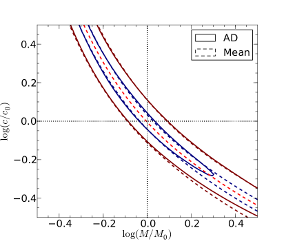
Figure 1: Constraints on the mass, $M$, and concentration, $c$, derived from 1000 particle realizations drawn from a model nfw halo. The outer (blue) and inner (brown) contours mark the 1 and 3$\sigma$ confidence regions respectively, for the mean phase (dashed) and AD (solid) estimators. The central red dashed line marks $\bar{\Theta}=0$. The parameters are expressed in units of the true parameter values, $M_{0}$ and $c_{0}$.

Even though the usefulness of these two statistics as estimators is severely limited by the strong degeneracies, they can still be used as theoretical probes to identify regions of discrepancy in heterogeneous data. In particular, the signed mean phase deviation as a standard normal variable is easy to calculate as well as being easy to interpret, making it a good residual measure of the phase distribution under the proposed potential. We demonstrate such an application in Section 6.2. Similar applications can be found extensively in paper II when analysing tracers from cosmological simulations.

4.2 Breaking the degeneracy: the radial likelihood estimator

In addition to the minimum distance estimators in $\theta$-space, we also try to construct maximum likelihood estimators. Since $\theta$ is not a direct observable but is model dependent, its PDF cannot be directly used to construct a likelihood. Instead, we work with the directly observable $r$-coordinate to calculate the likelihood of the observations, making use of the oPDF, $P(r|E,L)$. Since $E$ is unknown before the potential is known, trying to use the conditional probability ${\cal L}=\prod_{i}\mathrm{d}P(r_{i}|E_{i},L_{i})$ as a likelihood to infer the potential will fail. Since $P(E,L)$ is solely a characteristic property of the tracer (tracers with any arbitrary $P(E,L)$ can be constructed or selected) and is independent of the potential, one could seek to eliminate the $(E,L)$ dependence by marginalizing over their prior distributions.

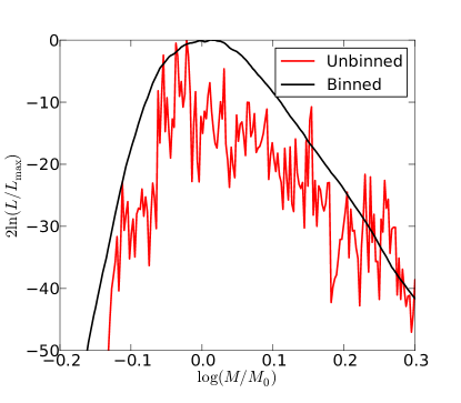
Figure 2: The radial likelihood function. We apply the unbinned (Eq. (30), red spiky curve) and binned (Eq. (31), black smooth curve) likelihood estimator to the same sample of 1000 ideal tracer particles in an NFW halo. The concentration parameter is fixed to be the true value and the likelihood is calculated as a function of the mass parameter, $M$, normalized by the true mass, $M_{0}$. The likelihood ratio, $2\ln({\cal L}/{\cal L}_{\rm max})$, is plotted where ${\cal L}_{\rm max}$ is the maximum likelihood value as the mass is varied. We adopt 30 bins logarithmically space between $1$ and $1000\,{\rm kpc}$ in radius in the binned case.

A proper marginalization can be done if one knows the $P(E,L)$ distribution. If one introduces additional assumptions on $P(E,L)$ (e.g., Bovy et al., 2010), then the method essentially reduces to a $f(E,L)$ method, whose generality is limited by the assumptions made. We would like to avoid any such assumptions in order to avoid any potential bias in the inferred potential introduced through them. Without prior knowledge of $P(E,L)$, we can approximate it with the observed distribution

$$\frac{\mathrm{d}^{2}P(E,L)}{\mathrm{d}E\mathrm{d}L}=\frac{1}{N}\sum_{i}\delta(E+K_{i}+\psi(r_{i}))\delta(L-L_{i}).$$ (24)

Now the marginalized distribution becomes:

$$\mathrm{d}P(r) =\int\mathrm{d}P(r|E,L)\,\frac{\mathrm{d}^{2}P(E,L)}{\mathrm{d}E\mathrm{d}L}\,dE\,dL$$ (25)

$$=\frac{1}{N}\sum_{i=1}^{N}\mathrm{d}P(r|E_{i},L_{i}).$$ (26)

This is the mixed (empirically marginalized) radial distribution, an analogy to the marginalized theoretical radial distribution. We can define a reciprocal probability of finding a particle at $r_{i}$ with the orbital parameters corresponding to ($E_{j},L_{j}$) as

$$P_{ij} =\frac{\mathrm{d}P(r_{i}|E_{j},L_{j})}{\mathrm{d}r_{i}}$$ (27)

$$=\frac{1}{v_{r}(r_{i},E_{j},L_{j})T_{j}}.$$ (28)

Then, the marginalized radial distribution becomes

$$\frac{\mathrm{d}P(r_{i})}{\mathrm{d}r_{i}}=\frac{1}{N}\sum_{j=1}^{N}P_{ij}.$$ (29)

This $P(r_{i})$ is actually the posterior probability of finding a particle at position $r_{i}$ given the orbital parameters of all the tracer particles, $P(r_{i}|E_{1},E_{2},...E_{N},L_{1},L_{2},...L_{N})$. Now the likelihood can be written as

$${\cal L}=\prod_{i=1}^{N}\sum_{j=1}^{N}P_{ij}.$$ (30)

However, the above likelihood function is very noisy. In Fig. 2, we show an example of this likelihood as a function of the halo mass parameter for the ideal tracer. Overall, the global shape of the likelihood function peaks around the true parameter value. On the other hand, the likelihood function is not at all smooth. Moreover, one does not get rid of this bumpiness by zooming into a finer grid in $M$. The noisy behaviour originates from the singularities in the PDF at peri and apo-centres, and from the discreteness in the $(E,L)$ distribution, which we described as a sum of $\delta$-functions. The noise in the likelihood can thus be regarded as Poisson noise. This Poisson noise prevents accurate inference of parameter values. Some form of smoothing can suppress the Poisson noise. For example, one could try to do kernel interpolation in the $(E,L)$ distribution, to make it a continuous rather than a discrete distribution (see e.g., Bovy et al., 2010; Magorrian, 2014). The simplest smoothing strategy would be to bin the data. If we bin the data radially into $m$ bins, then the binned version of the mixed radial likelihood can be written as

$${\cal L} =\prod_{i=1}^{m}\hat{n}_{i}^{n_{i}}\exp(-\hat{n}_{i})$$

$$=\exp\left(-\sum_{i}\hat{n}_{i}\right)\prod_{i=1}^{m}\hat{n}_{i}^{n_{i}}$$

$$=\exp(-N)\prod_{i=1}^{m}\hat{n}_{i}^{n_{i}},$$ (31)

where $n_{i}$ is the number of particles in the $i$-th bin. We have omitted the data-dependent constants in the above equation, and $\sum_{i}\hat{n}_{i}=N$ due to the normalization of the PDF. The predicted number of particles in the $i$-th bin is given by

$$\hat{n}_{i}=N\int_{r_{{\rm l},i}}^{r_{{\rm u},i}}\frac{\mathrm{d}P(r_{i})}{\mathrm{d}r_{i}}\,dr_{i},$$ (32)

where $r_{{\rm l},i}$ and $r_{{\rm u},i}$ are the lower and upper bin edges, and $P(r_{i})$ is given by equation (29). The binned likelihood curve is also shown in Fig. 2 for the same sample. Clearly, the Poisson noise has been suppressed and the likelihood function is now smooth and usable for parameter inference.

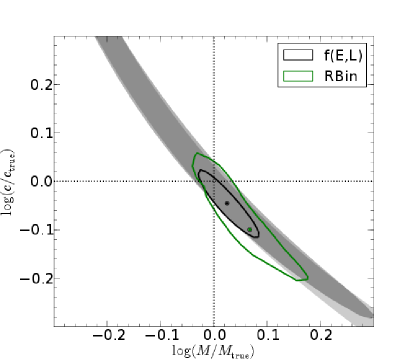
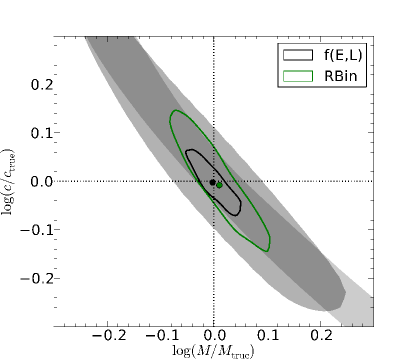
Figure 3: The $1\sigma$ confidence region for the different estimators. In both panels, the dark and light shaded regions are the confidence regions from the AD and mean-phase estimators respectively, while the green line marks the confidence region from the radial likelihood estimator (RBin), and the black line marks that from the $f(E,L)$ estimator. In the left panel, the confidence regions are inferred from a single sample of 1000 particles. The blue and black points correspond to the best-fit parameters of the radial likelihood and $f(E,L)$ estimators. In the right panel, the confidence regions represent the 68.3% most probable region of the best-fitting parameters, according to the distribution of best-fitting parameters from 750 independent samples. The blue and black points correspond to the average parameters from the radial likelihood and $f(E,L)$ estimators respectively. Note that since the AD and mean phase fits are sensitive to the initial guess of the parameter values due to their strong degeneracy, we have randomly picked the initial values when fitting each sample. The $f(E,L)$ and RBin fits are independent of the initial parameters. The samples used here are generated according to the $f(E,L)$ DF with true parameters $(M_{0},c_{0})$; hence the $f(E,L)$ fit is, by construction, the best constraint one can obtain.

In Fig. 3 we apply the binned radial likelihood estimator to the ideal tracers. In the left panel, the three estimators are applied to the single realization of 1000 particles used in Fig. 1. The degeneracy we have seen in the phase angle estimators is broken in the radial likelihood estimator. The estimators are applied to many (750) independent realizations of the same $f(E,L)$ distribution, and the distribution of the best-fit parameters are plotted in the right panel of Fig. 3. This test shows the estimator to be unbiased when averaged over many realizations. For comparison, we also show the result of a likelihood analysis using the full $f(E,L)$ distribution as in Wang et al. (2015). Note that since the data are generated with this exact DF, the $f(E,L)$ likelihood applied to these ideal tracers represent the best constraint one can get from any likelihood inference.

The radial likelihood estimator gives wider but still comparable confidence intervals as the full $f(E,L)$ estimator. Note that we have not assumed anything about the $(E,L)$ distribution of the tracers and that the mock catalogue is used blindly. The above test is a general demonstration that our method will work for any steady-state tracers in a static spherical potential. Compared to the perfect $f(E,L)$ method, where the adopted $f(E,L)$ exactly matches the form of the unknown underlying distribution function, the confidence interval is wider but, in practice, the $f(E,L)$ method will be biased if the tracer follows a $(E,L)$ distribution other than the specific $f(E,L)$ model adopted. With a small increase in noise, our radial likelihood method gains generality. Compared with the minimum distance estimators, the radial likelihood estimator breaks the degeneracy in the mass concentration parameters. Since the likelihood can be interpreted as the conditional probability of the data given the model, in principle it can also be adopted in an Bayesian analysis.

We now make a few comments on the practical application of the binned likelihood estimator. Since the purpose of the binning is purely to suppress shot noise, a larger number of bins is generally better, as long as it is not too noisy. On the other hand, when the likelihood contours appear too irregular, one should try reducing the number of radial bins to ensure the irregularities are not caused by shot noise. In our analysis, we have adopted 30 logarithmic bins for an ideal sample of 1000 particles, and 50 bins for $10^{6}$ particles in a realistic halo (paper II), although as few as 5 bins could still work. Due to the singularity of the $1/v$ integrand at orbital boundaries, it is expensive to achieve high accuracy for the phase calculations. As a result, it is difficult to use algorithms involving numerical derivatives for the optimization of the likelihood values. Instead, we adopt the Nelder-Mead simplex minimizer to search for the maximum of the likelihood.

5 Reconstructing the potential profile: the phase-mark non-parametric method

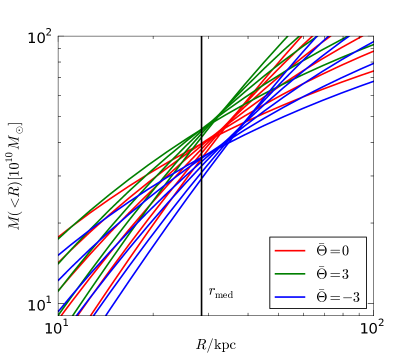
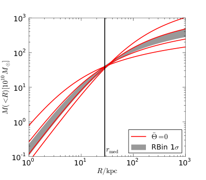
Figure 4: Constraints on the mass profile from different methods. In the left panel, we plot the predicted mass profiles adopting parameters lying on the $\bar{\Theta}=0$ and $\pm 3$ lines in the parameter space in Fig. 1 ($\bar{\Theta}=3,0,-3$ from top to bottom near the median radius). The vertical line marks the median radius (i.e., the half mass radius) of the tracer. In the right panel, the $\bar{\Theta}=0$ profiles are compared, over a wider radial range, with those adopting parameters on the $1\sigma$ contour of the binned radial likelihood estimator. The span of the latter, that is, the $1\sigma$ prediction bounds of the likelihood estimator, are marked by the shaded region. Note that since the constant $\bar{\Theta}$ lines are not closed in the parameter space (e.g., Fig. 1), there could be many mass profiles with shapes far more different from those plotted in this figure that still share the same $\bar{\Theta}$. In other words, the shape variation at the same $\bar{\Theta}$ could be much larger than plotted.

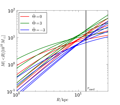
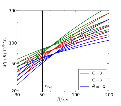
Figure 5: Mass profiles adopting parameters on constant $\bar{\Theta}$ lines, demonstrating the characteristic radius of the tracers. These are the same as the left panel of Fig. 4 but using two tracer samples with different radial cuts. The left panel uses a sample from $1-30~{}{\rm kpc}$, while the right panel uses a sample from $30-1000~{}{\rm kpc}$. The vertical black lines mark the half mass (i.e., median) radius of each sample. The sample sizes are both 1000 particles and are selected by applying only radial cuts to the parent samples constructed in Section 3.

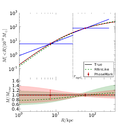
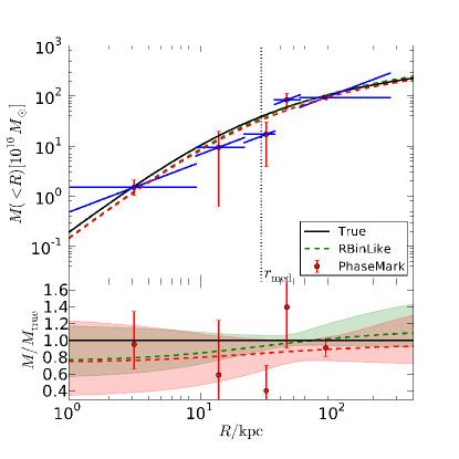
Figure 6: The mass profile constrained with the phase-mark method. The left and right panels are the same except that they have different number of radial bins. The bins are defined to have equal numbers of tracer particles, by subdividing a parent sample of 1000 particles. In each upper panel, the vertical dotted line marks the median radius of the full sample of tracers; the black solid line shows the true mass profile of the halo; the green dashed line is the best-fit profile using the radial likelihood method; the blue solid lines are the best-fit point-mass and isothermal profiles in each radial range. The point where the two blue lines cross (marked by points with error-bars) gives the characteristic mass in each bin. The errorbars are the uncertainty in the fitted point-mass parameter. The red dashed line is the best-fit NFW profile to the characteristic mass points. The bottom panels are the corresponding mass profiles divided by the true profile. The shaded region shows the $1$-$\sigma$ uncertainty on the fitted profiles from the radial likelihood (green) and from fitting NFW profiles to the characteristic masses (red).

5.1 Towards understanding the parameter degeneracy

The strong parameter degeneracy with the minimum distance estimators is easy to understand when we examine the constraints on the mass profile of the halo, as shown in Fig. 4. Parameters yielding the same mean phase deviation, $\bar{\Theta}$, all predict the same mass $M(<R_{\rm c})=M_{\rm c}$ inside a characteristic radius, $R_{\rm c}$, of the tracer, which is close to the half-mass radius of the tracer. Different $\bar{\Theta}$ values correspond to different $M(<R_{\rm c})$, with a positive correlation between the two. In other words, the mean phase of the tracer is an estimator of the gravitational force $GM(<R_{\rm c})/R_{\rm c}^{2}$ or circular velocity around the characteristic radius of the tracer population. On the other hand, this estimator barely constrains the gravity elsewhere, leaving the shape of the mass profile unconstrained. Parameters leading to the same $M(<R_{\rm c})$ but different shapes in the mass profile are thus indistinguishable by the mean phase estimator, resulting in the parameter degeneracy in Fig. 1. The radial likelihood estimator breaks this degeneracy by its ability to also constrain the shape of the profile, as illustrated in the right panel of Fig. 4.

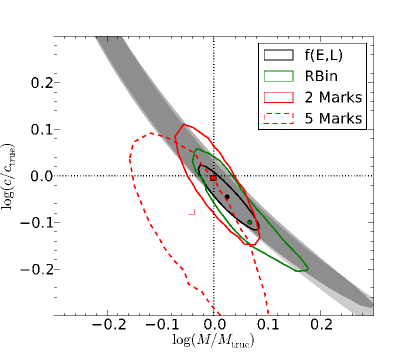
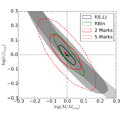
Figure 7: Same as Fig. 3, but also showing the constraints from fitting NFW profiles to the phase-marks. In the left panel, the red solid and red dashed contours show the $1$-$\sigma$ confidence regions obtained by dividing a single sample of 1000 particles into two and five radial bins respectively. The red filled and open squares in the centre of each contour show the corresponding best-fit parameters. In the right panel, the contours show the 68.3% most probable region of the best-fitting parameters, according to their distribution obtained from many (750) independent samples of 1000 particles each. The points in the centre show the median best-fitting parameters. Again the result for the phase-mark with two and five bins are shown in red solid and dashed contours respectively, while the filled and open squares show the corresponding median parameters.

The positive correlation between the mean phase $\bar{\Theta}$ and the characteristic mass, $M(<R_{\rm c})$, can be understood qualitatively. For profiles with the same shape (on a logscale), a higher $M(<R_{\rm c})$ leads to deeper potential everywhere. For a particle with a given position and velocity, a deeper potential of the same shape will shift both its peri and apocentres closer to the centre of the halo. As a result, the current location of the particle relative to its peri and apocentres is shifted outward, increasing its phase angle $\theta$. The mean phase of all particles thus increases with the characteristic mass.

The location of the characteristic radius determines the shape of the mean phase line in parameter space. To demonstrate this, instead of working in the $(M,c)$ parameter space, it is more convenient to work in the $(M_{\rm s},r_{\rm s})$ space, where $M_{\rm s}=4\pi\rho_{\rm s}r_{\rm s}^{3}$. Suppose the constant $\bar{\Theta}$ lines are described by $M_{\rm s}=f_{\bar{\Theta}}(r_{\rm s})$, then we have $M(<r)=f_{\bar{\Theta}}(r_{\rm s})[\ln(1+r/r_{\rm s})-(r/r_{\rm s})/(1+r/r_{\rm s})]$. Now the characteristic radius $r$ at which the mass does not vary with the halo parameter $r_{\rm s}$ is given by

$$\frac{\partial M(<r,r_{\rm s})}{\partial r_{\rm s}}=0,$$ (33)

whose solution $r=R_{\rm c}$ depends on the contour line function $f_{\bar{\Theta}}(r_{\rm s})$. So the functional form of the contour line determines $R_{\rm c}$, and vice versa.

It is worth clarifying that the characteristic radius, hence also the shape of the degeneracy curve, is determined by the distribution of the tracer and is not an intrinsic property of the halo. We demonstrate this in Fig. 5, where the characteristic radii of two ideal tracers with different radial ranges are shown. The two tracers are constructed by sampling from $1-30$ and $30-1000$ kpc respectively from a parent population whose half mass radius is roughly $30$ kpc. Clearly, the two samples have different characteristic radii, which are both close to their own half-mass radii, while the haloes hosting the two samples are identical. Correspondingly, we have checked that the mean phase contours have different slopes in $\log(M)-\log(c)$ space from that shown in Fig. 1.

The existence of a best-constrained mass despite the parameter degeneracy is broadly in line with empirical results on the robustness of the mass constraint inside the half-light radius from Jeans equation modelling of dwarf galaxies (Walker et al., 2009; Wolf et al., 2010). The existence of such a characteristic point in the Jeans analysis is further proved by Wolf et al. (2010). However, their results are concerned with the insensitivity of the mass estimate to the velocity anisotropy parameter of the tracers, which has to be fitted or assumed because only line-of-sight velocities are available in these studies. On the other hand, our parameter degeneracy arises from solving the mean-phase equation using the full 6D data. Anisotropy is not a parameter in our model at all.

Another closely related result to ours is presented by Amorisco & Evans (2011, AE11 hereafter), who studied the underlying potential of dwarf spheroidals assuming a lowered isothermal DF. They found that the structural parameters $(\rho_{s},r_{s})$ (or $(\rho_{0},r_{0})$ in the original notation of AE11) of NFW-like haloes are constrained by the observed $(R_{\rm h},\sigma_{0})$ of each dwarf spheroidal to follow a certain relation, $\rho_{s}(r_{s})$, where $R_{\rm h}$ is the projected half-light radius and $\sigma_{0}$ is the line-of-sight velocity dispersion at the centre of the dwarf spheroidal. This resulted in a best-constrained mass near a common characteristic radius $R_{\rm c}=1.7R_{\rm h}$ for almost all the dwarf spheroidals. As we explained above (see Equation 33), the existence of this characteristic point can be understood because the two parameter halo profile is reduced to a one parameter family due to the constraint of the problem. In AE11, the constraint comes from matching the observed $(R_{\rm h},\sigma_{0})$ of each system. By contrast, in our case a constrained relation, $\rho_{s}(r_{s})$, or equivalently, $M(c)$, is determined by solving $\bar{\Theta}=0$ (see Fig. 1). Note that it is not expected that an arbitrary constraint (for example, $r_{s}(\rho_{s})=\rm{Const}$) would always result in a best-constrained mass in the mass profile, so the similarity between the results by AE11 and ours is intriguing. Despite the apparent similarity, our result is purely theoretical, while that of AE11 is empirically driven by the observed quantities, $(R_{h},\sigma_{0})$. Our finding is expected to apply to steady state tracers in general, not only to those described by the lowered isothermal DF or to the observed dwarf spheroidals studied in AE11. In our general case, the characteristic radius is not a constant value in units of the median radius, as is evident in Fig. 5. We checked that the same is true (i.e., the scale is not universal) in units of the projected half-mass radius. By contrast, the common characteristic radius in AE11 is likely to arise from some common properties shared by the dwarf spheroidals studied there, namely the tight correlation between $(R_{h},\sigma_{0})$.

5.2 The phase-mark method

The experiment in Fig. 5 also suggests a way of breaking the degeneracy in the mean-phase estimator, by applying it to two or more subsamples split in radius. In this way the shape of the mass profile can be constrained as well, since different subsamples constrain the characteristic mass, $M_{\rm c}$, at different radius, $R_{\rm c}$. For parametric fits, the degeneracy lines in Fig. 1 would have different slopes for subsamples with different $R_{\rm c}$, so they could jointly determine a unique best-fit parameter set. Even better than that, it is possible to reconstruct the mass profile non-parametrically, thanks to the insensitivity of the mean-phase constraint on the shape of the mass profile. The fact that the mean phase only depends on the characteristic mass point means one can start from a profile of an arbitrary shape and still obtain the correct characteristic mass, by requiring the profile to produce the correct mean phase. As a result, it is not necessary to know the functional form of the true profile in order to constrain $(R_{\rm c},M_{\rm c})$. By applying the mean-phase constraint $\bar{\Theta}=0$ twice to two different single-parameter profiles and looking for the point where they intersect, one can simultaneously obtain both the characteristic radius and the characteristic mass. Note that only having $M_{\rm c}$ is not enough, since $R_{\rm c}$ is unknown even though it is close to the tracer half-mass radius.

We demonstrate this in Fig. 6. In the left panel, we divide the tracer sample of 1000 particles studied in Fig. 9 into two sub-populations according to radius. Inside each bin, we fit two mass profiles with the mean-phase estimator: 1) point mass profile, $M(<R)=M_{\rm c}$ with parameter $M_{\rm c}$; 2) isothermal profile, $M(<R)=kR$, with parameter $k$. The mean phase constraint $\bar{\Theta}=0$ uniquely determines a best fit for each profile. As expected, they cross the true profile at the same point, which marks the characteristic point of that bin as ($R_{\rm c}=M_{\rm c}/k$, $M(<R_{\rm c})=M_{\rm c})$. We name this method the “phase-mark”. Splitting the tracer into more bins, we can obtain finer constraints on the profile, as shown in the right hand panel. By doing this, we have reconstructed the true mass profile non-parametrically, without any assumption on the true profile. Such reconstructed mass profile becomes noisier when a larger number of bins is adopted (right panel), since each subsample becomes smaller.

If desired, one can still fit a parametric function through the reconstructed profile, as shown by the red dashed line in each panel, with confidence regions on the fitted profile marked by the red shaded regions in the lower panels. After combining all the radial bins, the tightest constraint is still found near the half-mass radius of the full tracer sample. It is interesting to see that although a larger number of bins helps to obtain finer reconstruction of the profile, it does not lead to a better constrained profile after fitting. It appears that the constraining power using only two bins is close to that of the radial likelihood method. This is confirmed by the more direct comparisons made in Fig. 7. The confidence region of the phase-mark with two bins has a comparable size to that of the likelihood method. This means they are similarly efficient at making use of the dynamical information. Adopting finer bins in the phase-mark results in a looser constraint. This can be understood because each mark only exploits the local phase uniformity inside each radial bin, while the large scale variation from bin to bin is not taken into account, resulting in a leakage of information. A potential improvement would be to combine bins at different scales. However, it should be kept in mind that doing this will introduce correlations among the marks, making the error analysis difficult. In the right panel, the phase-mark with two bins is applied to many independent Monte-Carlo realizations of the same system as before, to show that the fit is statistically unbiased.

6 Discussion

6.1 What is a tracer population?

Dynamical modelling require the tracer sample to be defined first, or subsamples to be selected from a parent sample. Here we revisit the question of “what is a tracer population?”. Modelling the tracer population with a time-independent DF requires the tracers to be in a steady state. For a spherically symmetric potential, this requirement translates into a conditional radial distribution $dN/dr\propto{1}/{|v_{r}(E,L,r)|}$ (necessary and sufficient) given $E$ and $L$, or equivalently, all the particles have completely uncorrelated radial phases. Once this condition is satisfied, one can use the distribution of the sample to infer the potential of the system. As a result, we can simply define a tracer as any set of steady-state particles moving in the background potential.

To obtain a steady state subsample, the selection from the sample must not distort this conditional radial distribution and must avoid introducing artificial structure in the radial or angle distribution. As long as this is guaranteed, any selection in $E$ and $L$ is allowed. For example, one can select subregions of the $E-L$ space, while keeping full or random sampling in $r$. For a parent population not in equilibrium inside a static potential, a steady-state subsample can still be selected by sampling according to Eq (9).

From this definition we also learn how to mix tracers with weights. If tracer $i$ has a steady-state phase-space distribution $f_{i}$, then the uniformly weighted population $w_{i}f_{i}$ is still a tracer. Consequently, $N$ mixed tracers $\sum_{i=1}^{N}w_{i}f_{i}$ is still a tracer, since equation (9) is satisfied for every subtracer. As a result, when dealing with multi-component tracers using the oPDF, we can either model them as a single population, or as several populations separately.

Obviously, subhalo particles are not steady-state tracers since they are localized structures. Streams in general are also not steady state tracers since they are usually characterized by correlated phases.

6.2 The optimal marginalization

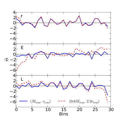
Figure 8: Mean phase profile evaluated with the two degenerating parameter sets. From top to bottom we bin the same sample of 1000 tracer particles according to their $r,E,L$ coordinates respectively, with equal number of particles in each bin. The mean phase deviation, $\bar{\Theta}$, is evaluated inside each bin. Different coloured lines represent different haloes. The blue solid and red dashed lines are the profiles adopting two different potentials: one with the real parameter values ($M,c$) and the other with a parameter set ($0.6M,2.2c$) whose mean phase is degenerate with that of the true parameters.

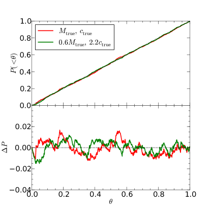
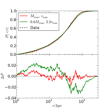
Figure 9: Cumulative distributions in $\theta$ and $r$ spaces. Left: Cumulative distribution of $\theta$, at two sets of parameter values. The red solid line corresponds to the true parameters, while the green solid line corresponds to ($0.6M,2.2c$) which give the same mean phase. The bottom panel is the difference between the model distribution and the cumulative distribution of a uniform distribution. Right: cumulative distribution of $r$. The black dashed line is the distribution of the data, while the red and green lines are for the true and alternatives parameters as in the left panel.

It is tempting to ask why the radial likelihood estimator works better than the phase estimators. Recall that the oPDF actually specifies both the randomness of the phase angle and the independence of such a distribution on the orbital parameters. That is, the phase distribution is not only uniform in general, but also uniform inside any $(E,L)$ bin. The oPDF also applies to any radial range, so the uniformity is expected for any region in the $(r,E,L)$ space. In Fig. 8 we examine the mean phase in subregions of the phase space. We divide the data into 30 equal-count bins in each dimension, and measure the mean phase inside each bin for a given potential. This mean phase value indicates the discrepancy of the data inside this subregion with uniform phase distribution. We do this for two mean phase degenerate points. For the true potential, $\bar{\Theta}$ is consistent with 0 everywhere. For the degenerate parameter set, we start to see a dependence on $(E,L)$, and $\bar{\Theta}$ is biased positively or negatively at different places in the $(E,L)$ space, even though the combined $\bar{\Theta}$ or the $\bar{\Theta}$ in $r$ space would still be close to 0. This test shows that there is still useful information beyond the uniform $\theta$ distribution, namely its $(E,L)$ dependence.

Since the minimum distance estimators do not examine the $(E,L)$ dependence, they have effectively marginalized over the $(E,L)$ distribution of tracers. One can rewrite the definition of the phase angle as

$$\theta(r,E,L)=P(<r|E,L).$$ (34)

From this point of view, the marginalization is done by working in the cumulative probability space of the tracers. Although the radial likelihood method also marginalizes over the $(E,L)$ distribution, the marginalization combines the oPDF from different $(E,L)$ orbits in a different (possibly optimal) way. This could result in a marginalized DF that is more sensitive to the discrepancies in the conditional distribution. In Fig. 9 we see that the radial distribution is indeed more sensitive, by examining the difference between empirical and expected cumulative distributions in $\theta$ and $r$ space.

6.3 Connection to other methods

Since $\mathrm{d}P(r,E,L)=\mathrm{d}P(r|E,L)\mathrm{d}P(E,L)$, the full phase-space distribution of tracers breaks into two parts. The orbital PDF is determined by dynamics, and reflects the underlying potential. The $P(E,L)$ part is simply a characteristic of the tracer not necessarily related to dynamics, and a sample with any form of $P(E,L)$ can be constructed which is still a valid tracer population. Any DF method has to make use of the $P(r|E,L)$ information in some way, but how one deals with $P(E,L)$ is not crucial to the determination of the potential.

6.3.1 Comparison with the $f(E,L)$ DF method

As we have already discussed in Section 2.4, any $f(E,L)$ DF function has to be consistent with the oPDF, while imposing extra assumptions on the distribution of orbits. Because our method only uses the conditional radial distribution, it is fully compatible with the density profile inverted $f(E,L)$ method. At the same time, our method has no extra assumptions and is applicable to more general tracers. Also note that the density profile inversion involving a particular parametrization of the potential can sometimes be quite challenging  (see, e.g., Wang et al., 2015), and may not always be solvable analytically. In contrast, the application of any potential function in our oPDF method is always straightforward.

Since the oPDF is given in differential form, it does not care about the radial limits of the system. One can apply the orbital PDF to data within any radial range, e.g., from $r_{\rm min}$ to $r_{\rm max}$, since the phase-space continuity equation holds within any radial range. When radial cuts are imposed, we only need to replace the orbital limits $r_{\rm a}$ with $\max(r_{\rm a},r_{\rm min})$ and $r_{\rm p}$ with $\min(r_{\rm p},r_{\rm max})$. In this case, the data only care about the variation of the potential within the same radial range. For the same reason, the zero point of the potential, the extension of the halo or tracer density profile outside the data window, or the boundary of the halo is irrelevant in our method. By contrast, in the $f(E,L)$ method, the DF, $f(E,L)$, has to satisfy the radial constraint $\rho(r)=\int f(E,L)d^{3}v$ at all $r$ by definition. Any change in $\rho(r)$ at any radius will require an adjustment in the proposed DF. As a result, one has to include the full radial range of each orbit in its density profile inversion. This requires a full description of both the potential and the tracer density over the full radial range, introducing a dependence on quantities outside the data window. Such dependence, in turn, requires one to parametrize the tracer and the potential profiles for extrapolation. In particular, for a finite size system the boundary condition, $\rho(r_{\rm max})=0$, requires that no orbit should extend beyond $r_{\rm max}$, which translates into an energy bound, $E<-\phi(r_{\rm max})$. In other words, the energy of particles has to be bound for a finite size system described by $f(E,L)$. This constraint is the main cause of the poor match between model and data for simulated DM particles in  (Wang et al., 2015). This constraint does not apply to our method, however, because we do not need to study the full radial range of every orbit. For example, our method can be applied to an open system with constant inflows and outflows! In this sense, the oPDF is more general than Jeans theorem.

Fitting with a full DF also has its advantage over the general oPDF method. The prior assumptions on the distribution of orbits serve to input extra information to the model. If these assumptions are correct, the fitting can be more efficient, as demonstrated by the performance of the true $f(E,L)$ DF fitted to the ideal tracers. On the other hand, incorrect assumptions are likely to lead to biased results in the fits. From this point of view, adding extra assumptions in the construction of a DF is a trade-off between efficiency and correctness. Our oPDF method is specifically designed to minimize extra assumptions hence maximizing correctness.

6.3.2 Connection to Schwarzschild’s method

Our radial likelihood method can be regarded as a lightweight Schwarzschild’s method. Starting from the oPDF, $P(r|E,L)$, one can populate different orbits with tracer particles given a potential, and look for weighted combinations of orbits that reproduce the observed spatial distribution of the tracer. The best match then gives an estimate of both the potential and a phase-space distribution in the form of combinations of orbits. This is the exactly the Schwarzschild method (Schwarzschild, 1979), which essentially converts the $\rho=\int fd^{3}v$ into linear equations in phase-space grids $\rho(I)=\sum_{J}C(J)P(I|J)$, where $I$ denotes configuration grids and $J$ denotes orbit populations. However, to infer the potential, it is not necessary to solve for a general combination of orbits, $C(J)$. Instead, one can obtain the distribution of orbits directly from the observed phase-space positions of particles, with each particle determining one orbit, i.e, $C(J)=1$ with $J$ ranging from 1 to the number of particles. This is exactly what we do in our likelihood method. In this sense, our likelihood method is a special type of Schwarzschild’s method, with the population of orbits constrained to be the distribution of orbits in the data, rather than constructed from an external library. We do not lose generality with our choice of orbits, while hugely reducing the dimension of the problem by not solving for $C(J)$ at all.

The disadvantage of not fitting for the distribution of orbits in our method is that we have to rely on the full phase-space data to initialize each orbit. When only certain moments of the DF such as the velocity dispersion profile are available, Schwarzschild’s method can still be applied by fitting the predicted moments of the proposed DF to the observed ones, while the radial likelihood method constructed here cannot. Another advantage of the general Schwarzschild modelling is that it can be adopted to construct a self-gravitating equilibrium system, which can be used as initial conditions for N-body experiments.

6.4 Generalization of the likelihood method

Observational data usually involve selection functions describing the non-uniform sample completeness, noise in the measurements of the phase-space coordinates, and even missing dimensions in the coordinates. We briefly discuss how these complexities can be handled in the oPDF framework, as well as generalizations to non-spherical potentials. Given that the focus of this paper is to explore whether a general dynamical method is applicable to simulated haloes for the inference of the halo potential, we do not push the following discussions further to implementation. Instead, we leave further tests and improvements of the proposed solutions to future work. In the following, we will focus on the likelihood estimator as an example.

6.4.1 Selection function, noise, missing dimensions

As we have discussed before, our methods apply to tracers with any $(E,L)$ distribution, and hence is immune to any selection in $(E,L)$. Radial selection can be easily handled by modifying the reciprocal probability as

$$P_{ij}^{\prime}=\frac{P_{ij}S_{i}/S_{j}}{\int P_{ij}S_{i}/S_{j}\,dr_{i}},$$ (35)

where $S_{i}=S(r_{i})$ is the probability of selecting a particle into the sample at $r_{i}$ . If the selection is simply a radial cut, then equation (35) simplifies to an adjustment of the normalization factor $T$. When angular selections are involved, one needs to explicitly consider $\vec{L}$ instead of $L$ as the orbital parameters, to model the distribution in $r,\theta,\phi$ rather than just $r$.

The noise in the data can be incorporated as priors. Formally, the new likelihood after marginalizing over the error distribution can be written as

$$\mathcal{L}^{\prime}_{\psi}(D_{o})=\int\mathcal{L}_{\psi}(D)P(D|D_{o})dD,$$ (36)

where $\mathcal{L}_{\psi}(D)$ is the likelihood of an error-free dataset, $D$, in a potential $\psi$, $P(D|D_{o})$ is the probability that the true dataset is $D$ given the observed dataset $D_{o}$. Alternatively, one can generate Monte-Carlo realizations of the data according to the prior distributions, $P(D|D_{o})$, and apply the method to each realization assuming no noise in the measurements. Once this is done, a statistical estimate of the effect of the measurement noise on the fits can be obtained from the distribution of the best-fitting parameters across the different realizations.

Observational data might also miss some dimensions. For example, it is difficult to measure the tangential velocity for distant stars in the Galaxy. If only $v_{r}$ is available, then it is necessary to introduce additional assumptions on $v_{t}$ in order to apply the method, e.g., through an anisotropy parameter or anisotropy profile, $\beta(r)$.

6.4.2 Generalization to arbitrary potentials

For a non-spherical potential, it might be difficult to write down the integrals of motion as orbital parameters. However, the orbit is still fully determined for each particle once a potential is assumed, and one can calculate the orbit numerically without knowing the integrals of motion. With calculable orbits, we can still predict the spatial distribution of particles by superimposing the oPDF of each particle, and compare with the observed distributions for a likelihood analysis of the potential.

7 Conclusions

We have shown that tracers in a steady state in a static potential can be characterized by an orbit-dependent distribution function, $\mathrm{d}P(\lambda|{\rm orbit})\propto\mathrm{d}t(\lambda)$, with $\lambda$ being an affine parameter of the position along the orbit. This is a general result that follows from the time-independent collisionless Boltzmann equation. We clarify that the phase-space distribution of tracers connects to their host potential only through this oPDF, while the distribution of orbits, e.g., $P(E,L)$, is a characteristic of each tracer that is independent of the host potential. The oPDF can also be shown to be equivalent to Jeans theorem, which is the starting point for constructing DFs for steady-state tracers in most previous studies.

Starting solely from this oPDF, we have developed a likelihood estimator to infer the potential of a spherically symmetric halo. The method improves over previous $f(E,L)$ DF methods in making no assumption about the tracer characteristic functions, $P(E,L)$. We achieve this by approximating the prior distribution of orbits, $P(E,L)$, by their empirical distribution once a halo potential is assumed, and marginalize over this distribution. The approximation of $P(E,L)$ by its empirical version introduces strong shot noise, which is suppressed by binning the data radially.

To test the performance of the likelihood estimator we have created Monte-Carlo samples of steady-state tracers from a realistic phase-space DF for Milky Way halo stars. The DF of these samples is constructed to be in a steady state but also makes additional assumptions about the orbit population. Applying our estimator to these samples, we find it to be unbiased. Comparing our estimates with those from a likelihood estimator that uses the correct form of the underlying full DF, our estimated errorbars are only increased slightly ($\sim 20\%$), while avoiding having to assume any functional form for the DF. Such a likelihood estimator can be easily embedded into a Bayesian framework.

Expressed in action-angle coordinates, the oPDF reduces to the random phase principle proposed in BL04, which has been used to construct minimum distance estimators of the potential. When applied to the inference of an NFW potential, the minimum distance estimators suffer from a strong degeneracy in halo parameters, reflecting the fact that they only constrain the halo mass inside a tracer-specific radius. While this degeneracy is an obvious disadvantage of these methods, it also opens a door to non-parametric reconstruction of the potential profile (or rotation curve) due to its independence on the shape of the proposed profile. Taking advantage of this shape-independence, we have developed a non-parametric “phase-mark” method to reconstruct the potential profile, by fitting elementary profiles to radially split subsamples of the tracer to mark the characteristic mass in each radial bin. Applied to the Monte-Carlo samples, we have shown that the phase-mark correctly reconstructs the true potential without making any assumptions about its shape. Such reconstructed profiles can be further fitted to provide parametric constraints on the potential. We find that the constraining power of such fits can be as good as that of the likelihood method and the tightest constraint is obtained with only two radial subsamples. The phase-mark method is more intuitive for recovering the potential profile due to its non-parametric nature. It is also computationally much faster.

Both the likelihood estimator and the phase-mark are able to break the degeneracy between mass and concentration and constrain the shape of the halo mass profile over a large radial range. The generality of the oPDF also means that our methods can be applied to tracers with multiple components, but without the necessity of modelling each component separately. In the current form, the new methods developed in this paper can serve as a powerful tool to study the dynamical status of simulated haloes. They also offer a promising way to constrain the mass of the Milky Way halo with real data, once further extended and tested to work with observational errors and incompleteness.

Appendix A AD distribution

The theoretical distribution of the AD distance (Eq. 22) under the null hypothesis can be calculated with Monte-Carlo simulations. Specifically, we generate a number of independent random samples, and calculate the AD distance, $D$, for each of them. Each sample consists of $N$ independent observations of a uniformly distributed variable $\theta\in[0,1]$. In Fig. 10, we show that the distribution of $\ln(D)$ (Eq. 22) can be well fit by the sum of two normal distributions of the form

$$P\left(\ln{D}\right)=w\mathcal{N}\left(\ln{D},\mu_{1},\sigma_{1}\right)+(1-w)\mathcal{N}\left(\ln{D},\mu_{2},\sigma_{2}\right),$$ (37)

where $\mathcal{N}\left(x,\mu,\sigma\right)$ is the standard normal probability function of $x$ with mean $\mu$ and standard deviation $\sigma$. The best fit parameters are $w=0.569$, $\mu_{1}=-0.570$, $\sigma_{1}=0.511$, $\mu_{2}=0.227$, $\sigma_{2}=0.569$. Compared with the fitting function in BL04 designed to fit the tail of the distribution, the bi-normal PDF fits well the whole range of the distribution, which is important for likelihood analysis.

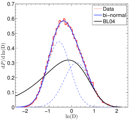
Figure 10: Binormal fit to the distribution of the AD statistic. The data are generated from an ensemble of $50\,000$ random samples, of size $N=5000$ each. For each of these samples, the AD statistic, $D$, is calculated. The empirical distribution of $\ln(D)$ is plotted as a histogram. The solid line passing through the histogram is a bi-normal fit according to Equation (37), which is the sum of two Gaussian components (dashed lines). For comparison, we also plot the BL04 fit which is only designed to describe the tail of the distribution.

The distribution has barely any dependence on the sample size $N$. For systems as small as $N=5$, we find our fitting still describes the empirical AD distribution very well. We also verified that the mean phase distribution can be well approximated by the normal distribution, for systems with $N\geq 5$.

References

- Amorisco & Evans (2011) Amorisco N. C., Evans N. W., 2011, MNRAS, 411, 2118, arXiv:1009.1813
- An & Evans (2009) An J. H., Evans N. W., 2009, ApJ, 701, 1500, arXiv:0906.3673
- Anderson & Darling (1954) Anderson T. W., Darling D. A., 1954, Journal of the American Statistical Association, 49, 765
- Bartelmann (2010) Bartelmann M., 2010, Classical and Quantum Gravity, 27, 233001, arXiv:1010.3829
- Beloborodov & Levin (2004) Beloborodov A. M., Levin Y., 2004, ApJ, 613, 224, astro-ph/0405533
- Binney & Mamon (1982) Binney J., Mamon G. A., 1982, MNRAS, 200, 361
- Binney & Tremaine (2008) Binney J., Tremaine S., 2008, Galactic Dynamics: Second Edition. Princeton University Press
- Bovy et al. (2010) Bovy J., Murray I., Hogg D. W., 2010, ApJ, 711, 1157, arXiv:0903.5308
- Camm (1952) Camm G. L., 1952, MNRAS, 112, 155
- Cooper et al. (2010) Cooper A. P. et al., 2010, MNRAS, 406, 744, arXiv:0910.3211
- Courteau et al. (2014) Courteau S. et al., 2014, Reviews of Modern Physics, 86, 47, arXiv:1309.3276
- Cuddeford (1991) Cuddeford P., 1991, MNRAS, 253, 414
- Eddington (1916) Eddington A. S., 1916, MNRAS, 76, 572
- Evans & An (2006) Evans N. W., An J. H., 2006, Phys. Rev. D, 73, 023524, astro-ph/0511687
- Han et al. (2014) Han J. et al., 2014, ArXiv e-prints, arXiv:1404.6828
- Han et al. (2015) Han J., Wang W., Cole S., Frenk C. S., 2015, ArXiv e-prints, arXiv:1507.00771
- Magorrian (2014) Magorrian J., 2014, MNRAS, 437, 2230, arXiv:1303.6099
- Merritt (1985) Merritt D., 1985, AJ, 90, 1027
- Navarro et al. (1996) Navarro J. F., Frenk C. S., White S. D. M., 1996, ApJ, 462, 563, arXiv:astro-ph/9508025
- Navarro et al. (1997) Navarro J. F., Frenk C. S., White S. D. M., 1997, ApJ, 490, 493, arXiv:astro-ph/9611107
- Osipkov (1979) Osipkov L. P., 1979, Soviet Astronomy Letters, 5, 42
- Posti et al. (2015) Posti L., Binney J., Nipoti C., Ciotti L., 2015, MNRAS, 447, 3060, arXiv:1411.7897
- Schwarzschild (1979) Schwarzschild M., 1979, ApJ, 232, 236
- Springel et al. (2008) Springel V. et al., 2008, MNRAS, 391, 1685, arXiv:0809.0898
- Walker et al. (2009) Walker M. G., Mateo M., Olszewski E. W., Peñarrubia J., Wyn Evans N., Gilmore G., 2009, ApJ, 704, 1274, arXiv:0906.0341
- Wang et al. (2015) Wang W., Han J., Cooper A., Cole S., Frenk C., Cai Y., Lowing B., 2015, ArXiv e-prints, arXiv:1502.03477
- Wilkinson & Evans (1999) Wilkinson M. I., Evans N. W., 1999, MNRAS, 310, 645, astro-ph/9906197
- Williams & Evans (2015a) Williams A. A., Evans N. W., 2015a, ArXiv e-prints, arXiv:1508.02584
- Williams & Evans (2015b) Williams A. A., Evans N. W., 2015b, MNRAS, 448, 1360, arXiv:1412.4640
- Wojtak et al. (2008) Wojtak R., Łokas E. L., Mamon G. A., Gottlöber S., Klypin A., Hoffman Y., 2008, MNRAS, 388, 815, arXiv:0802.0429
- Wolf et al. (2010) Wolf J., Martinez G. D., Bullock J. S., Kaplinghat M., Geha M., Muñoz R. R., Simon J. D., Avedo F. F., 2010, MNRAS, 406, 1220, arXiv:0908.2995