Geometric Phases for Mixed States
of the Kitaev Chain

Abstract

The Berry phase has found applications in building topological order parameters for certain condensed matter systems. The question whether some geometric phase for mixed states can serve the same purpose has been raised, and proposals are on the table. We analyze the intricate behaviour of Uhlmann’s geometric phase in the Kitaev chain at finite temperature, and then argue that it captures quite different physics from that intended. We also analyze the behaviour of a geometric phase introduced in the context of interferometry. For the Kitaev chain, this phase closely mirrors that of the Berry phase, and we argue that it merits further investigation.

1 Introduction

Quantum theory offers a rich supply of mathematical concepts, and, in principle, each of these raises the question of its physical interpretation. The geometric phase is an interesting example of such a concept as new applications of various geometric phases continue to appear. We have discussed this circle of ideas before, in rather general terms [1, 2]. Here our intention is to see how they play out in a context with specific demands on the interpretation.

The Berry phase for pure states has found application in the study of topologically ordered matter, and recently there has been some discussion [3, 4, 5, 6, 7] about the use of geometric phases for mixed states, and the role they can play, when topologically ordered matter is kept at finite temperature. In this paper we analyze the behaviour of two geometric phases for mixed states—Uhlmann’s phase [8, 9, 10] and the inequivalent [11] interferometric phase [12, 13]—in the Kitaev chain, which is a simple model that can undergo a topological phase transition. For the Uhlmann phase, we find a behaviour that is surprisingly intricate. However, we will eventually argue that the behaviour is not really tied to the physics we want to capture. In contrast to the Uhlmann phase, the interferometric geometric phase adopts a topological character and makes a discrete jump when the multiplicity of the spectrum of the state changes. In our calculation, this translates into a jump when the band gap closes in the Kitaev chain. Thus it is potentially a useful topological invariant, and we will argue that it deserves further study in the context.

The paper is organized as follows. In Section 2, we introduce the Kitaev chain and its associated Gibbs states, and in Sections 3 and 4 we define and analyze Uhlmann’s geometric phase for these. Section 5 contains a contrasting analysis of the interferometric phase, and Section 6 contains a discussion and our conclusions.

2 The Kitaev chain

A brief introduction to topological phases of matter may begin by reminding the reader that phases of matter have been very successfully understood by means of the concept of a local order parameter, as in Landau’s theory. The new twist is that in certain materials the order parameter may take on a global, topological character. Indeed, the issue here is whether some particular geometric phase can serve as an order parameter for a topological phase.

Let us consider a simple model known as the Kitaev chain [14] in which such behaviour can be seen. It is a $1$-dimensional model built from spinless fermions ($a_{n}a_{m}^{\dagger}+a_{m}^{\dagger}a_{n}=\delta_{nm}$) at $N$ sites with the Hamiltonian

$$H=\sum_{n=1}^{N}\left[-w(a_{n}^{\dagger}a_{n+1}+a_{n+1}^{\dagger}a_{n})-\mu a_{n}^{\dagger}a_{n}+M(a_{n}a_{n+1}+a_{n+1}^{\dagger}a_{n}^{\dagger})\right].$$ (1)

Here $w$ is the hopping amplitude, $\mu$ is the chemical potential and $M$ is known as the induced superconducting gap. We assume that the number of sites is large and that periodic boundary conditions are used.

We can use a Fourier transformation to reexpress the Hamiltonian as

$$H=\int_{0}^{2\pi}\frac{\operatorname{d}\!k}{2\pi}\Psi_{k}^{\dagger}H_{k}\Psi_{k},$$ (2)

where the Nambu spinor is $\Psi_{k}=(a_{k},a_{-k}^{\dagger})^{\rm T}$ and

$$H_{k}=-M\sin{k}\sigma_{y}-\left(\frac{\mu}{2}+w\cos{k}\right)\sigma_{z}.$$ (3)

The eigenvalues of this Hamiltonian are

$$\lambda_{\pm}=\pm\sqrt{\left(\frac{\mu}{2}+w\cos{k}\right)^{2}+\left(M\sin{k}\right)^{2}}.$$ (4)

Here, to simplify matters, we will set $w=M=1$ and $m=\mu/2$. Moreover, for convenience, we will represent the Hamiltonian so that the Bloch vector lies in the equatorial plane. Thus, we consider Hamiltonians of the form

$$H_{k}=-\frac{\Delta_{k}}{2}\vec{n}_{k}\cdot\vec{\sigma},$$ (5)

where $\vec{\sigma}=(\sigma_{x},\sigma_{y},\sigma_{z})$ are the Pauli matrices and

$$\vec{n}_{k} =\frac{2}{\Delta_{k}}\left(m+\cos{k},\sin{k},0\right),$$ (6)

$$\Delta_{k} =2\sqrt{(m+\cos{k})^{2}+\sin^{2}{k}}.$$ (7)

What is the physics of this? The model has two energy bands (which is why we can treat it as a qubit), with a band gap that closes if $m=1$. See Fig. 1. Kitaev found that in an open chain with a finite number of sites, the model behaves very differently depending on whether $m<1$ or $m>1$. In the former case, there are two extra states within the gap, which turn out to be exponentially localized on the edges of the chain. In the latter case, these states are missing. In this sense, there is a kind of phase transition at $m=1$.

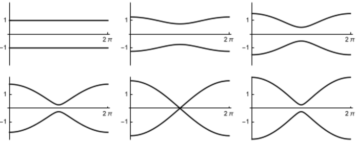
Figure 1: The spectra for $\Delta_{k}$ as in Eq. (7) and $m=0,1/4,2/4$ from left-to-right in the top row and $m=3/4,1,5/4$ from left-to-right in the bottom row. The fact that it matters whether $m$ is larger or smaller than one is not yet apparent.

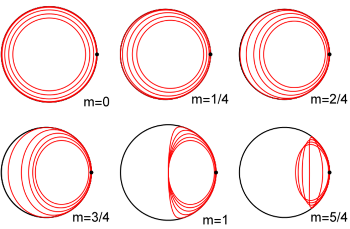
Figure 2: Curves in the Bloch ball for some values of $m$. In each panel, we see the curves swept out by the Gibbs states as we move along the Brillouin zone for $T=1/5,2/5,3/5,4/5,1$. The east pole is marked with a dot.

In our model, we can discern a topological order parameter by looking at the Bloch vector (6). As we move along the Brillouin zone, parameterized by $k$, the eigenstates move around the equator of the Bloch sphere for $m<1$, whereas for $m>1$ they are rocking back and forth around the east pole. In the former case, we pick up a Berry phase factor $e^{i\pi}$; in the latter case, the Berry phase is zero [15, 16, 17]. For $m=1$, the gap closes and the Berry phase is ill-defined. Thus, we can say that there is a topological $\mathbb{Z}_{2}$ invariant taking different values in the two phases, and this invariant serves as the order parameter of the model. A systematic classification of non-interacting models of this kind is available [18, 19, 20, 21].

After this (absurdly brief) introduction to topological phases of matter, we can go on to ask about mixed states. Assume that the chain is in contact with a thermal bath at temperature $T$, and is described by the Gibbs state

$$\rho(k)=\frac{e^{-H_{k}/T}}{\mbox{Tr}e^{-H_{k}/T}}=\frac{1}{2}\left(\mathbbm{1}+\tanh{\frac{\Delta_{k}}{2T}}\vec{n}_{k}\cdot\vec{\sigma}\right).$$ (8)

This state defines a curve within the equatorial plane of the Bloch ball, as shown in Fig. 2 for various values of $m$ and $T$. These curves can be described analytically. Using polar coordinates on the equatorial plane we have for the angular coordinate that

$$\varphi(k)=\frac{k}{2}+\arctan{\left(\frac{1-m}{1+m}\tan{\frac{k}{2}}\right)}.$$ (9)

The case $m=0$, which is called the flat band case, is particularly simple because the Brillouin zone is mapped to circles centred at the maximally mixed state. For $m<1$ the curves enclose, for $m=1$ the curves pass through and for $m>1$ the curves are confined to one side of the maximally mixed state.

The question now is if we can define a phase factor for mixed states, analogous to the Berry phase for pure states, which can serve as a topological invariant describing the phase structure of the Kitaev chain at finite temperature. The work by Viyuela et al. [3, 5] at first sight suggests that the Uhlmann geometric phase [8] can play this role. It would further suggest that there is a sharp transition between different phases of the model also at finite $T$, and that this transition happens at an $m=m_{c}(T)<1$. For curves in the equatorial plane of the Bloch ball the Uhlmann phase factor is indeed a number $\pm 1$ which can be calculated, and by fixing the curves in this manner Viyuela et al. have added an intriguing amount of concreteness to its study. We will add some more, and discuss its interpretation afterwards. We will also broaden the perspective slightly and study the behaviour of another candidate geometric phase for mixed states [12]. A paper with a similar aim has appeared recently [7].

3 The Uhlmann phase factor

The basic idea in Uhlmann’s theory is to let the pure states in the bipartite Hilbert space $\mathcal{H}\otimes\mathcal{H}^{\star}$ form the total space of a fiber bundle over the mixed states on $\mathcal{H}$, see Ref. [10]. The projection onto the mixed states is $\psi\rightarrow\psi\psi^{\dagger}=\rho$, and the structure group is $U(N)$ acting from the right, $\psi\rightarrow\psi U$. A geometric phase can be associated to any curve in the base manifold once we have defined a parallelism condition for curves in the total space—a lift $\psi(k)$ of $\rho(k)$ is said to be parallel if for every infinitesimal $\delta k$ the probability for the transition from $\psi(k)$ to $\psi(k+\delta k)$ equals the fidelity of $\rho(k)$ and $\rho(k+\delta k)$,

$$\left|\operatorname{Tr}(\psi(k)^{\dagger}\psi(k+\delta k))\right|^{2}=\operatorname{Tr}\sqrt{\rho(k)^{1/2}\rho(k+\delta k)\rho(k)^{1/2}}.$$ (10)

The parallelism condition can also be described in terms of a connection [22], which we here denote by $\mathcal{A}$. In general, no explicit formula for $\mathcal{A}$ is known. However, Hübner [23] has derived a formula giving its values along the velocity fields of ’square root lifts’ $\psi=\sqrt{\rho}$. The formula of Hübner reads

$$\mathcal{A}(\dot{\psi})=\sum_{i,j}|u_{i}\rangle\frac{\langle u_{i}|[\dot{\psi},\psi]|u_{j}\rangle}{p_{i}+p_{j}}\langle u_{j}|,$$ (11)

where the $p_{i}$ and the $|{u_{i}}\rangle$ are the eigenvalues and eigenstates of $\rho$, and the overdot means differentiation with respect to $k$. It should be pointed out that the derivation of (11) assumes that $\rho$ has full rank, so it fails when the system is in a pure state. Indeed, the Uhlmann bundle is defined for mixed states of full rank only. Apart from that, it is insensitive to the spectra of the mixed states.

Let us postpone a discussion of the physical import of Uhlmann’s construction and turn directly to an evaluation of the Uhlmann phase for curves in the equatorial plane of the Bloch ball. In general, Hübner’s formula (11) is hard to handle, but for the qubit state space it simplifies to

$$\mathcal{A}(\dot{\psi})=(\sqrt{p_{1}}-\sqrt{p_{2}})^{2}(|u_{1}\rangle\langle u_{1}|\dot{u}_{2}\rangle\langle u_{2}|+|u_{2}\rangle\langle u_{2}|\dot{u}_{1}\rangle\langle u_{1}|).$$ (12)

Since $\rho$ depends on $k$, so do its eigenvectors $|{u_{i}}\rangle$ and its eigenvalues $p_{i}$. We are interested in curves that stay in the equatorial plane of the Bloch ball, and set

$$\rho=\frac{1}{2}\begin{pmatrix}1&(p_{1}-p_{2})e^{-i\varphi}\\ (p_{1}-p_{2})e^{i\varphi}&1\end{pmatrix}$$ (13)

and

$$|{u_{1}}\rangle=\frac{1}{\sqrt{2}}\begin{pmatrix}1\\ e^{i\varphi}\end{pmatrix},\qquad|{u_{2}}\rangle=\frac{1}{\sqrt{2}}\begin{pmatrix}1\\ -e^{i\varphi}\end{pmatrix}.$$ (14)

Then the connection becomes abelian,

$$\mathcal{A}(\dot{\psi})=\frac{i}{2}\dot{\varphi}(\sqrt{p_{1}}-\sqrt{p_{2}})^{2}\begin{pmatrix}-1&0\\ 0&1\end{pmatrix},$$ (15)

and no path ordering is necessary in order to compute the symmetry group element

$$U(k)=\exp\left(-\int_{0}^{k}\!\operatorname{d}\!k\,\mathcal{A}(\dot{\psi})\right)=\begin{pmatrix}e^{iA}&0\\ 0&e^{-iA}\end{pmatrix},$$ (16)

where

$$A=\frac{1}{2}\int_{0}^{k}\!\operatorname{d}\!k\,\dot{\varphi}(\sqrt{p_{1}}-\sqrt{p_{2}})^{2}.$$ (17)

A parallel lift of $\rho(k)$, then, is

$$\psi_{||}(k)=\psi(k)U(k)=\frac{1}{2}\begin{pmatrix}(\sqrt{p_{1}}+\sqrt{p_{2}})e^{iA}&(\sqrt{p_{1}}-\sqrt{p_{2}})e^{i(A-\varphi)}\\ (\sqrt{p_{1}}-\sqrt{p_{2}})e^{i(\varphi-A)}&(\sqrt{p_{1}}+\sqrt{p_{2}})e^{-iA}\end{pmatrix}.$$ (18)

The unitary $U(k)$ depends on the special lift we started out with, $\psi=\sqrt{\rho}$, but $\psi_{||}(k)$ does not. Let us remark—since it will be important to us later on—that $\psi_{||}(k)$ is in general not periodic, even if the original curve $\rho(k)$ is closed with periodicity $2\pi$. The function $A(k)$ need not be periodic even if $\varphi(k)$ is.

Uhlmann’s geometric phase is the argument of the phase factor of the function

$$\begin{split}\operatorname{Tr}\left(\psi_{||}(0)^{\dagger}\psi_{||}(k)\right)&=\frac{1}{2}\Big{(}\sqrt{p_{1}(0)}+\sqrt{p_{2}(0)}\Big{)}\Big{(}\sqrt{p_{1}(k)}+\sqrt{p_{2}(k)}\Big{)}\cos{A}\,+\\ &+\frac{1}{2}\Big{(}\sqrt{p_{1}(0)}-\sqrt{p_{2}(0)}\Big{)}\Big{(}\sqrt{p_{1}(k)}-\sqrt{p_{2}(k)}\Big{)}\cos{(\varphi+A)}.\end{split}$$ (19)

Because we consider curves in the equatorial plane of the Bloch ball, this is a real-valued quantity. For small values of $k$ therefore the phase factor equals $+1$, and it stays that way until we reach a node on the curve, that is, a point where the trace vanishes. At a non-degenerate node the phase factor jumps to $-1$. If the curve was deformed slightly away from the equatorial plane we would see the phase building up continuously around the position of the node.

4 Concrete behaviour of the Uhlmann phase factor

We now specialize to the case of Gibbs states of the Kitaev chain, for which

$$p_{1}=\frac{1}{2}\big{(}1+\tanh{\frac{\Delta_{k}}{2T}}\big{)},\qquad p_{2}=\frac{1}{2}\big{(}1-\tanh{\frac{\Delta_{k}}{2T}}\big{)}.$$ (20)

To simplify matters we consider one of two cases, either the flat band case ($m=0$, $\Delta_{k}=2$) or the case of closed curves (using $\Delta_{0}=\Delta_{2\pi}$). In either case $p_{i}(k)=p_{i}(0)=p_{i}$, and Eq. (19) simplifies. We find that

$$(\sqrt{p_{1}}+\sqrt{p_{2}})^{2}=1+\operatorname{sech}\frac{\Delta_{k}}{2T},\qquad(\sqrt{p_{1}}-\sqrt{p_{2}})^{2}=1-\operatorname{sech}\frac{\Delta_{k}}{2T}.$$ (21)

Before inserting this result into Eq. (19), we define

$$x=\operatorname{sech}\frac{\Delta_{k}}{2T}.$$ (22)

Recalling that Uhlmann’s phase factor is multiplied by a factor $-1$ each time the curve encounters a node, we see that the task is to find those values of $k$ for which

$$\operatorname{Tr}\left(\psi(0)^{\dagger}\psi(k)U(k)\right)=\frac{1}{2}\left((1+x)\cos{A}+(1-x)\cos{(\varphi+A)}\right)=0.$$ (23)

In this equation, $x=x(k;T)$ as $x$ depends on $\Delta_{k}$, and moreover

$$A=A(k;T)=\frac{1}{2}\int_{0}^{k}\!\operatorname{d}\!k\,\dot{\varphi}(1-x).$$ (24)

In general this integral is too hard for us to do analytically.

We first consider the simplest case, the flat band case in which $\Delta_{k}=2$, $x=\operatorname{sech}(1/T)$ and

$$A=\frac{\varphi}{2}(1-x).$$ (25)

The curves are then circles, and the temperature alone determines the purity of the states. The limit $T\to 0$ can now be taken. When $T=0$ the hyperbolic secant vanishes, the state is pure, $A=\varphi/2$ and the nodes are determined by the equation

$$\cos{\frac{\varphi}{2}}+\cos{\frac{3\varphi}{2}}=0\quad\Leftrightarrow\quad\cos{\frac{\varphi}{2}}\left(\cos^{2}{\frac{\varphi}{2}}-\frac{1}{2}\right)=0.$$ (26)

Hence there are nodes at $\varphi=\pi/2,\pi,3\pi/2$. This should be compared with the the Berry phase, which has a single node at $\varphi=\pi$. However, for a closed circle the contributions from the two extra nodes will cancel each other, and we obtain the same value for the Uhlmann and Berry phases (as noted by Uhlmann [8]).

To see what happens as we increase $T$, that is to say as we shrink the radii of the circles, refer to Fig. 3a.

(a) At most one turn.

(b) Between one and two turns.

Figure 3: Where the nodes lie if the paths start on the positive $x$-axis and go counterclockwise along circles of constant purity.

The first thing that happens is that the two ’extra’ nodes between $\pi/2$ and $\pi$ disappear. Then there is a value of $T$ (called the ’critical temperature’ by Viyuela et al. [3]) for which the circle coincides with the dashed circle. For higher values of $T$ no nodes are encountered during the first revolution around the Brillouin zone, and consequently Uhlmann’s phase factor remains equal to $+1$. But the evolution of the purified state $\psi_{||}(k)$ is not periodic in $k$, so a node will be encountered during the second revolution (unless the temperature is so high that we are inside the smaller dashed circle), see Fig. 3b, and so on.

Fig. 4

Figure 4: Solutions of Eq. (23) for $\Delta_{k}=2$ and winding numbers up to 5, with $x=$ sech$(1/T)$ as the ordinate. For large $T$, that is for high entanglement, the circles traversed in the Bloch ball are small and several revolutions are needed to see a node.

gives the location of the nodes for as many as 5 revolutions. The curves defining the nodes reflect the rather complicated evolution of $\psi_{||}(k)$. However, by inspection we see that some periodicities appear if we consider closed curves. The condition for a node to occur after exactly $n_{1}$ revolutions is

$$\cos\left(A(2\pi n_{1})\right)=\cos((1-x)n_{1}\pi)=0.$$ (27)

There are $n_{1}$ solutions for $n_{1}$ revolutions, namely

$$x_{n_{1},n_{2}}=\frac{2(n_{1}-n_{2})-1}{2n_{1}},\qquad n_{2}\in\{0,1,\dots,n_{1}-1\}.$$ (28)

The node at $x=1/2$ repeats after two more revolutions since

$$x_{1,0}=x_{3,1}=x_{5,2}=\dots=\frac{1}{2}.$$ (29)

For open curves no special simplifications are visible.

Going beyond the flat band case is a more involved story. We first ask for what value of $T$ we have a node occurring after exactly one turn. This means that we have to solve the equation

$$\cos{(A(T))}=0,\qquad A(T)=\frac{1}{2}\int_{0}^{2\pi}\!\operatorname{d}\!k\,\dot{\varphi}(1-x(k,T)).$$ (30)

This is a straightforward Mathematica calculation, and the result is reported in Fig. 5a.

(a) The location of the ’critical temperature’ $T_{cr}=T_{1,0}$ after one turn, in agreement with [3].

(b) Location of critical temperatures $T_{n_{1},n_{2}}$ for $n_{1}=1$, 2 and 3 turns.

Figure 5: Location of critical temperatures $T_{n_{1},n_{2}}$ for $n_{1}=1$, 2 and 3 turns. Compare with Fig. 4, which shows the flat band case only. The dashed line in panel (a) gives the size of the band gap (with Boltzmann’s constant set to $1$).

The resulting curve is in fact a cross-section of any one out of the three two dimensional figures given by Viyuela et al. [3] (their Figure 2, which is considerably more beautiful than ours). They interpret the resulting values of $T$—less than half of the bandgap at $m=0$—as an $m$-dependent critical temperature at which something dramatic happens to the Kitaev chain. We can, however, easily complicate matters by asking for the value of $T$ for which we have a node occurring after exactly two turns, or three turns and so on. Following this logic, we would then seem to be led to the conclusion that there is something dramatic happening to the Kitaev chain at finite temperature also for values of $m$ which exceed 1. See Fig. 5b. It is therefore necessary to reexamine the physical logic behind the Uhlmann phase, and we do so in Section 6.

5 The interferometric geometric phase

In Ref:s. [12, 13], a different geometric phase for mixed quantum states was introduced in the context of interferometry. Its general definition is fairly involved, but for mixed states having non-degenerate spectra, which is the only case considered here, the definition can be seen as a straightforward generalization of the Berry phase for pure states.

Consider a curve of density operators

$$\rho(k)=\sum_{i}p_{i}(k)|u_{i}(k)\rangle\langle u_{i}(k)|$$ (31)

such that for each $k$, the eigenvalues $p_{i}(k)$ are non-degenerate. If the eigenstates develop in a parallel manner,

$$\langle u_{i}(k)|\dot{u}_{i}(k)\rangle=0,$$ (32)

we define the interferometric geometric phase of $\rho(k)$ as

$$\gamma(k)=\arg\sum_{i}\sqrt{p_{i}(0)p_{i}(k)}\langle u_{i}(0)|u_{i}(k)\rangle.$$ (33)

As for Uhlmann’s phase, the interferometric phase does not depend on the operator that determines the dynamics of the system. Rather, it is a quantity associated with $\rho(k)$ which only depends on how $\rho(k)$ is embedded in the space of density operators. However, this is true only if the eigenstates satisfy the parallelism condition (32). If this condition is not met, we need to phase-shift the eigenstates as follows:

$$|{u_{i}(k)}\rangle\to|{u_{i}(k)}\rangle e^{-\int_{0}^{k}\operatorname{d}\!l\langle u_{i}(l)|\dot{u}_{i}(l)\rangle}.$$ (34)

Clearly, the interferometric geometric phase reduces to the Berry phase if $\rho(k)$ is a curve of pure states.

The Berry phase for a cyclically evolving pure state equals half of the solid angle enclosed by the curve traced out by the state’s Bloch vector on the Bloch sphere. Using this observation, it is fairly easy to calculate the interferometric phase for cyclically evolving qubits, provided they do not pass the maximally mixed state. In fact, we believe that the parallelism condition in Eq. (32) cannot be extended to include all curves that pass through the maximally mixed state. However, this is still under investigation.

Consider a closed curve of mixed qubits

$$\rho(k)=p_{1}(k)|u_{1}(k)\rangle\langle u_{1}(k)|+p_{2}(k)|u_{2}(k)\rangle\langle u_{2}(k)|,\qquad(0\leq k\leq\kappa),$$ (35)

and assume that the eigenvectors $|{u_{i}(k)}\rangle$ satisfy the parallelism condition (32). Let $\vec{R}(k)$ be the Bloch vector of $\rho(k)$, and let $\vec{r}(k)=\vec{R}(k)/R(k)$, where $R(k)$ is the Euclidean length of $\vec{R}(k)$. Then $\vec{r}(k)$ is a closed curve on the Bloch sphere and $\langle u_{1}(0)|u_{1}(\kappa)\rangle=e^{i\theta_{1}}$, where $\theta_{1}$ equals half of the solid angle enclosed by $\vec{r}(k)$. Furthermore, $\langle u_{2}(0)|u_{2}(\kappa)\rangle=e^{i\theta_{2}}$, where $\theta_{2}$ is half of the solid angle enclosed by the curve $-\vec{r}(k)$. Accordingly, $e^{i\theta_{2}}=e^{-i\theta_{1}}$, and the interferometric geometric phase of $\rho(k)$ can be written as

$$\gamma(\kappa)=\arg(p_{1}(0)e^{i\theta_{1}}+p_{2}(0)e^{-i\theta_{1}})=\arg(\cos\theta_{1}+iR(0)\sin\theta_{1}).$$ (36)

We observe, in particular, that for the planar curves defined by (13) and indexed by $m$, the interferometric phase is $0$ if the curve has an even winding number with respect to the maximally mixed state, and equals $\pi$ if the winding number is odd, see Fig. 2. When $m=1$, however, the interferometric phase is undefined. Thus, it signals a closing of the band gap for the Kitaev chain in the same way as the Berry phase, but at a finite temperature.

An analysis like the one conducted for Uhlmann’s phase shows that the interferometric geometric phase has nodes along the radial segment in the Bloch ball opposite to the initial state. For the curves given by (13) this means that each point on the negative $x$-axis is a node, as shown in Fig. 6.

Figure 6: The nodes of the interferometric phase are situated on the radial segment opposite to the initial state. No build-up of the phase occurs before and after the passage of a node. If the curve passes the line of nodes, the phase makes a sudden $\pi$-jump.

There is no phase build-up before, or after, the curve reaches a node. But at the node, the interferometric phase factor gets multiplied by $-1$. In this sense the behaviour of the interferometric phase closely mirrors that of the Berry phase.

6 Discussion and conclusion

We have been concerned with the physical interpretation, in a definite context, of two different geometric phases for mixed states—the Uhlmann and the interferometric phases. Following the earlier studies [3, 5, 6, 7], we have analyzed their behaviour to see if they are indicators of topological phases of matter at finite temperature. As our test case we have used the Kitaev chain, a one-dimensional system of non-interacting electrons which gives rise to a curve of Gibbs states in an equatorial plane of the Bloch ball as we move along the Brillouin zone.

When $T=0$, and the Kitaev chain is in a pure state, the Berry phase is a topological invariant which takes different values around $m=1$ where the system undergoes a topological phase transition. For $m<1$ the state is in a topologically non-trivial phase admitting localized zero-energy edge states, and the Berry phase factor is $-1$. For $m>1$ there are no localized edge states and the Berry phase factor is $+1$. At finite temperature, on the other hand, the Kitaev chain is in a mixed state. Now, both of the mixed state geometric phase factors considered take the values $\pm 1$, but for the Uhlmann phase factor the behaviour is quite complex. We are not aware of a physical interpretation of the Uhlmann phase itself, but indeed the Uhlmann phase behaves in a way that may be of interest, regardless of the proposed interpretation of the states. Here it should be recalled that Uhlmann’s theory was designed with very different ends in view. It can be argued that Uhlmann’s $U(N)$ bundle is as natural a construction for mixed states as is the unit sphere in Hilbert space considered as a $U(1)$ bundle over the set of pure states. They both have major implications for the probabilistic structure of quantum mechanics [10]. For example, Uhlmann’s construction gives rise to a metric which is monotone under stochastic maps [24, 25], and plays an important role in statistical inference [26]. It must also be mentioned that the Uhlmann phase is measurable in experiments where the purified state appears as a bipartite entangled state including a system and a controlled ancilla [27, 28, 29]—but this is a very different situation from that of a system in contact with a thermal bath having a huge number of uncontrollable degrees of freedom.

What we found, when considering the concrete curves under study, was first of all an interesting, but in the context devastating, ’memory effect’. The phase changes along these curves occur only at certain nodes, and the locations of these nodes depend on how many turns around the curve have been made already. Another observation concerns the limiting behaviour of the Uhlmann phase as the curve approaches the pure state boundary, which corresponds to letting the temperature approach zero. The Berry phase is recovered for closed curves [8], but for open curves this is not the case. The argument is delicate because Uhlmann’s bundle does not extend over the states of less than maximal rank (which play a special role in statistical inference).

We now turn to the relevance of the Uhlmann phase for the condensed matter application we have in mind. Our first observation is that the Uhlmann phase is insensitive to the closure of the band gap. More precisely, if $T>0$ and we let $m$ approach $1$ from below, we see that the Uhlmann phase changes its value before we reach $m=1$, see Fig. 5a. When $m=1$, the band gap is closed, and the curve traversed by $\rho(k)$ passes through the maximally mixed state. However, this does not affect Uhlmann’s geometric phase. In standard discussions of the topological origin of the edge states such behaviour of an invariant is explicitly forbidden (see, for instance, Ref. [30]). Furthermore, Fig. 5b shows that the Uhlmann phase behaves in a very non-trivial fashion for a range of temperatures also when $m>1$, in which case the chemical potential is in the non-topological range. We therefore agree with Viyuela et al. [3] when they state that the Uhlmann phase “does not determine the fate of the edge modes at finite temperature”. The Uhlmann phase was simply designed for a different purpose.

In the spirit of Budich and Diehl [7], we have also looked at a different geometric phase for mixed states, one that is sensitive to changes of the multiplicities in the spectra of the states. For the interferometric geometric phase, the phase factor is $-1$ for odd number of revolutions in the Brillouin zone and $+1$ for even numbers, no matter what the temperature is. This means that the interferometric phase does not detect any phase transition in temperature, but it detects the same phase transition as the Berry phase for pure states, i.e. at $m=1$. In fact, it extends the Berry phase to finite temperature in a way that captures the periodicity of the state of the Kitaev chain. For $\rho(k)$ given by Eq. (13), modeling pure states if $T=0$ and mixed states if $T>0$, induces a homomorphism between the fundamental groups of the Brillouin zone with end points identified and the equatorial plane punctured at the maximally mixed state. Both of these groups equal the group of integers, $\mathbb{Z}$, and the homomorphism is $n\to dn$ where $d$ is the degree of the Bloch vector. (Thus, $d=1$ if $m<1$ and $d=0$ if $m>1$.) We can extend this with a second homomorphism $\mathbb{Z}\to\mathbb{Z}_{2}$ sending $n$ to $e^{in\pi}$. Here $\mathbb{Z}_{2}$ denotes the multiplicative group of the two elements $\pm 1$. The composite homomorphism $n\to e^{idn\pi}$ is the topological invariant given by the Berry phase for $T=0$ and the interferometric phase for $T>0$. Observe that the non-periodicity, due to the memory effect mentioned above, excludes the possibility of extracting a similar invariant from Uhlmann’s geometric phase.

To summarize, the Uhlmann geometric phase is part of a general construction of great importance and import in quantum mechanics, but we see no reason for why it should be useful as an indicator of topological order in models resembling the Kitaev chain. The interferometric geometric phase on the other hand seems to be more appropriate as a topological order parameter at finite temperature, and we think it merits further investigation in the context of condensed matter.

References

References

- [1] E. Sjöqvist. Pancharatnam revisited. Quantum Theory: Reconsideration of Foundations, ed. A. Y. Khrennikov; series “Math. Modelling in Physics, Engineering and Cognitive Sciences”, Växjö Univ. Press, 2002.
- [2] I. Bengtsson. Geometrical statistics—classical and quantum. Quantum Theory: Reconsideration of Foundations, eds. G. Adenier, A. Khrennikov; T. M. Nieuwenhuizen, AIP Conf. Proc., 810:59-66, 2006.
- [3] O. Viyuela, A. Rivas and M. A. Martin-Delgado. Uhlmann phase as a topological measure for one-dimensional fermion systems. Phys. Rev. Lett., 112:130401, 2014.
- [4] O. Viyuela, A. Rivas and M. A. Martin-Delgado. Two-dimensional density-matrix topological fermionic phases: Topological Uhlmann numbers. Phys. Rev. Lett., 113:076408, 2014.
- [5] O. Viyuela, A. Rivas and M. A. Martin-Delgado. Symmetry-protected topological phases at finite temperature. 2D Mater., 2:034006, 2015.
- [6] Z. Huang and D. P. Arovas. Topological indices for open and thermal systems via Uhlmann’s phase. Phys. Rev. Lett., 113:076407, 2014.
- [7] J. C. Budich and S. Diehl. Topology of density matrices. Phys. Rev. B, 91:165140, 2015.
- [8] A. Uhlmann. Parallel transport and ’quantum holonomy’ along density operator. Rep. Math. Phys., 24(2):229–240, 1986.
- [9] A. Uhlmann. On Berry phases along mixtures of states. Ann. Phys., 501(1):63–69, 1989.
- [10] A. Uhlmann and B. Crell. Geometry of state spaces, Lecture Notes in Physics volume 768. Springer, Berlin, 2009.
- [11] P. B. Slater. Geometric phases of the Uhlmann and Sjöqvist et al. types for -orbits of -level Gibbsian density matrices. arXiv:math-ph/0112054, 2001.
- [12] E. Sjöqvist, A. K. Pati, A. Ekert, J. S. Anandan, M. Ericsson, D. K. L. Oi and V. Vedral. Geometric phases for mixed states in interferometry. Phys. Rev. Lett., 85:2845–2849, 2000.
- [13] D. M. Tong, E. Sjöqvist, L. C. Kwek and C. H. Oh. Kinematic approach to the mixed state geometric phase in nonunitary evolution. Phys. Rev. Lett., 93:080405, 2004.
- [14] A. Y. Kitaev. Unpaired Majorana fermions in quantum wires. Phys. Usp., 44(10S):131, 2001.
- [15] M. V. Berry. Quantal phase factors accompanying adiabatic changes. Proc. R. Soc. Lond. A, 392(1802):45–57, 1984.
- [16] Y. Aharonov and J. Anandan. Phase change during a cyclic quantum evolution. Phys. Rev. Lett., 58:1593–1596, 1987.
- [17] J. Zak. Berry’s phase for energy bands in solids. Phys. Rev. Lett., 62:2747–2750, 1989.
- [18] A. P. Schnyder, S. Ryu, A. Furusaki and A. W. W. Ludwig. Classification of topological insulators and superconductors in three spatial dimensions. Phys. Rev. B, 78:195125, 2008.
- [19] X.-L. Qi, T. L. Hughes and S.-C. Zhang. Topological field theory of time-reversal invariant insulators. Phys. Rev. B, 78:195424, 2008.
- [20] A. Y. Kitaev. Periodic table for topological insulators and superconductors. AIP Conf. Proc., 1134(1):22–30, 2009.
- [21] S. Ryu, A. P. Schnyder, A. Furusaki and A. W. W. Ludwig. Topological insulators and superconductors: tenfold way and dimensional hierarchy. New J. Phys., 12(6):065010, 2010.
- [22] A. Uhlmann. A gauge field governing parallel transport along mixed states. Lett. Math. Phys., 21(3):229–236, 1991.
- [23] M. Hübner. Computation of Uhlmann’s parallel transport for density matrices and the Bures metric on three-dimensional Hilbert space. Phys. Lett. A, 179(4-5):226–230, 1993.
- [24] A. Uhlmann. The metric of Bures and the geometric phase. In Quantum groups and related topics (Wrocław, 1991), Volume 13 of Math. Phys. Stud., pages 267–274. Kluwer Acad. Publ., Dordrecht, 1992.
- [25] D. Petz. Monotone metrics on matrix spaces. Linear Algebra Appl., 244:81–96, 1996.
- [26] S. L. Braunstein and C. M. Caves. Statistical distance and the geometry of quantum states. Phys. Rev. Lett., 72:3439–3443, 1994.
- [27] M. Ericsson, A. K. Pati, E. Sjöqvist, J. Brännlund and D. K. L. Oi. Mixed State Geometric Phases, Entangled Systems, and Local Unitary Transformations. Phys. Rev. Lett., 91:90405, 2003.
- [28] J. Åberg, D. Kult, E. Sjöqvist and D. K. L. Oi. Operational approach to the Uhlmann holonomy. Phys. Rev. A, 75:032106, 2007.
- [29] J. Zhu, M. Shi, V. Vedral, X. Peng, D. Suter and J. Du. Experimental demonstration of a unified framework for mixed-state geometric phases. Europhys. Lett., 94(2):20007, 2011.
- [30] S. Ryu and Y. Hatsugai. Topological origin of zero-energy edge states in particle-hole symmetric systems. Phys. Rev. Lett., 89:077002, 2002.