A SPECTROSCOPIC ANALYSIS OF THE GALACTIC GLOBULAR CLUSTER NGC 6273 (M19)

Abstract

A combined effort utilizing spectroscopy and photometry has revealed the existence of a new globular cluster class. These “anomalous” clusters, which we refer to as “iron–complex” clusters, are differentiated from normal clusters by exhibiting large ($\gtrsim$0.10 dex) intrinsic metallicity dispersions, complex sub–giant branches, and correlated [Fe/H] and s–process enhancements. In order to further investigate this phenomenon, we have measured radial velocities and chemical abundances for red giant branch stars in the massive, but scarcely studied, globular cluster NGC 6273. The velocities and abundances were determined using high resolution (R$\sim$27,000) spectra obtained with the Michigan/Magellan Fiber System (M2FS) and MSpec spectrograph on the Magellan–Clay 6.5m telescope at Las Campanas Observatory. We find that NGC 6273 has an average heliocentric radial velocity of $+$144.49 km s^-1 ($\sigma$=9.64 km s^-1) and an extended metallicity distribution ([Fe/H]=–1.80 to –1.30) composed of at least two distinct stellar populations. Although the two dominant populations have similar [Na/Fe], [Al/Fe], and [$\alpha$/Fe] abundance patterns, the more metal–rich stars exhibit significant [La/Fe] enhancements. The [La/Eu] data indicate that the increase in [La/Fe] is due to almost pure s–process enrichment. A third more metal–rich population with low [X/Fe] ratios may also be present. Therefore, NGC 6273 joins clusters such as $\omega$ Centauri, M 2, M 22, and NGC 5286 as a new class of iron–complex clusters exhibiting complicated star formation histories.

1. INTRODUCTION

Galactic globular clusters are proving to be a rich and diverse population. These objects are generally older than about 10 Gyr ($\sigma$$\sim$3 Gyr; e.g., Rosenberg et al. 1999; Salaris & Weiss 2002; De Angeli et al. 2005; Marín–Franch et al. 2009; VandenBergh et al. 2013), but also span about a factor of 300 in metallicity (e.g., Zinn & West 1984; Harris 1996; Carretta & Gratton 1997; Kraft & Ivans 2003; Carretta et al. 2009a). Early high resolution spectroscopic work revealed that clusters typically contain stars with similar heavy element abundances, most notably [Fe/H], but with $>$0.5–1.0 dex star–to–star abundance variations for elements lighter than about Si (e.g., Cohen 1978; Peterson 1980; Sneden et al. 1991; Kraft et al. 1992; Pilachowski et al. 1996; Gratton et al. 2001). Furthermore, it was discovered that the light element abundance variations are (anti–)correlated with one another, and that the correlation patterns, such as the O–Na anti–correlation and Na–Al correlation, are evidence that the gas from which the present–day low mass globular cluster stars formed was subjected to high–temperature proton–capture nucleosynthesis (e.g., Denisenkov & Denisenkova 1990; Langer et al. 1993; Prantzos et al. 2007). Except for a few notable cases (Koch et al. 2009; Caloi & D’Antona 2011; Villanova et al. 2013), recent large sample spectroscopic surveys (e.g., Carretta et al. 2009b,c) have built upon this early work and cemented the idea that the correlated light element abundance variations are a characteristic common to perhaps all Galactic globular clusters (see also reviews by Kraft 1994; Gratton et al. 2004; 2012). These spectroscopic observations provided the first evidence that globular clusters may not be simple stellar populations.

Concurrent with spectroscopic work has been the revelation that, when observed using appropriate filter combinations, the color–magnitude diagrams of many globular clusters exhibit multiple, often discreet, photometric sequences that can extend from the main–sequence to the asymptotic giant branch (AGB; e.g., Piotto et al. 2007, 2012, 2015; Lardo et al. 2011; Milone et al. 2012a,b, 2015; Monelli et al. 2013; Cummings et al. 2014; Lim et al. 2015). Since many of the filters used are sensitive to a star’s light element composition (e.g., Bond & Neff 1969), the combined spectroscopic evidence of large star–to–star light element abundance variations and photometric evidence of multiple color–magnitude diagram sequences reveals that nearly all clusters host more than one stellar population. For clusters exhibiting a negligible spread in [Fe/H], the various populations are often categorized by their light element chemistry as “primordial”, “intermediate”, or “extreme” stars (e.g., Carretta et al. 2009c). The primordial stars are thought to be the first generation and have a composition similar to halo field stars (high [O/Fe] and low [Na/Fe]), and the intermediate stars are thought to be second generation stars that exhibit lower [O/Fe] and higher [Na/Fe]. Only a small number of clusters host extreme stars, which are distinguished as having [Na/Fe]$\gtrsim$$+$0.4 and [O/Fe]$\lesssim$–0.2. The intermediate population dominates by number in most clusters (Carretta et al. 2009c), and the intermediate and extreme stars may also have enhanced He relative to the primordial population (e.g., Bragaglia et al. 2010; Dupree et al. 2011; Pasquini et al. 2011; Mucciarelli et al. 2014).

While spectroscopic and photometric analyses provide clear evidence that more than one stellar population, differentiated by light element chemistry, exists within most globular clusters, no consensus has yet been reached regarding the cause of the light element variations nor its interpretation. The sole stable argument in the debate about globular cluster composition is that, outside of normal dredge–up processes, the light element abundance variations were largely already imprinted on the gas from which the stars formed. This result is most clearly evidenced by observations of unevolved main–sequence and sub–giant branch (SGB) stars exhibiting the same light element correlations as the red giant branch (RGB) stars (e.g., Briley et al. 1996; Gratton et al. 2001; Cohen & Meléndez 2005; Bragaglia et al. 2010; D’Orazi et al. 2010; Dobrovolskas et al. 2014). However, the available data make differentiating various pollution scenarios difficult. To date, none of the proposed nucleosynthesis sources, which include intermediate mass ($\sim$5–8 M_⊙) AGB stars (e.g., Fenner et al. 2004; Karakas et al. 2006; Ventura & D’Antona 2009; D’Ercole et al. 2010; Ventura et al. 2013; Doherty et al. 2014), massive rapidly rotating main–sequence stars (e.g., Decressin et al. 2007; 2010), interacting massive binary stars (de Mink et al. 2009; Izzard et al. 2013), and very massive ($\sim$10⁴ M_⊙) stars (Denissenkov & Hartwick 2014), are able to fully explain all observed abundance patterns. Additionally, no combination of the previously proposed sources seems able to reproduce all abundance patterns either (Bastian et al. 2015). A formal merging of the spectroscopic and photometric observations with theoretical models remains a work in progress.

Although the measured [Fe/H] dispersion is $\lesssim$12$\%$ ($\lesssim$0.05 dex) for many globular clusters (Carretta et al. 2009a), a population of about 8 known clusters exists for which the derived [Fe/H] spread exceeds the measurement errors (e.g., see Marino et al. 2015; their Table 10). These “anomalous” clusters, which we refer to as “iron–complex” clusters, are often identified by the following features: (1) a dispersion in [Fe/H] exceeding $\sim$0.10 dex when measured using moderately high dispersion and signal–to–noise ratio (S/N) spectra, (2) multiple photometric sequences, especially on the SGB, and (3) a significant abundance spread for light elements and also heavy elements that, in the Solar System, are produced by the slow neutron–capture process (s–process). Many iron–complex clusters are also relatively massive and tend to host very blue horizontal branches (HB). The massive globular cluster omega Centauri ($\omega$ Cen) is the best known and most extreme object from this group, and has been demonstrated by multiple authors to possess: a very blue HB, a range in [Fe/H] that spans about a factor of 100, at least five distinct main stellar populations (each with its own set of primordial, intermediate, and extreme stars), and a strong correlation between metallicity and elements such as Ba and La that are likely produced by the s–process (e.g., Norris & Da Costa 1995; Suntzeff & Kraft 1996; Lee et al. 1999; Smith et al. 2000; Bellini et al. 2010; Johnson & Pilachowski 2010; D’Orazi et al. 2011; Marino et al. 2011a; Pancino et al. 2011; Villanova et al. 2014). Less extreme examples also include M 22, M 2, M 54, NGC 1851, NGC 5286, NGC 5824, and Terzan 5 (M 22: e.g,. Hesser et al. 1977; Pilachowski et al. 1982; Lehnert et al. 1991; Marino et al. 2009, 2011b, 2013; Da Costa et al. 2009; Roederer et al. 2011; Alves–Brito et al. 2012; M 2: Piotto et al. 2012; Lardo et al. 2013; Yong et al. 2014; Milone et al. 2015; M 54: e.g., Sarajedini & Layden 1995; Brown et al. 1999; Siegel et al. 2007; Bellazzini et al. 2008; Carretta et al. 2010a; NGC 1851: e.g., Yong & Grundahl 2008; Milone et al. 2009; Yong et al. 2009, 2015; Zoccali et al. 2009; Carretta et al. 2010b, 2011; NGC 5286: Marino et al. 2015; NGC 5824: Saviane et al. 2012; Da Costa et al. 2014; Terzan 5: Ferraro et al. 2009; Origlia et al. 2011, 2013; Massari et al. 2014). Among these clusters, $\omega$ Cen, M 22, M 2, and NGC 5286 stand out because each has been confirmed to host at least two stellar populations distinguished by their [Fe/H] and s–process abundances.

In this context, we examine here the chemical composition of RGB stars in the globular cluster NGC 6273 (M19), which is a scarcely studied cluster near the Galactic bulge. NGC 6273 is one of the most massive and luminous clusters in the Galaxy (M_V=–9.13; M$\sim$1.2–1.6$\times$10⁶ M_⊙; Harris 1996; Gnedin & Ostriker 1997; Brown et al. 2010), and despite suffering from significant differential reddening has shown some evidence supporting the existence of a metallicity spread and complex color–magnitude diagram (Harris et al. 1976; Rutledge et al. 1997; Piotto et al. 1999, 2002; Brown et al. 2010; Alonso–García et al. 2012). A possible spread in color on the RGB and an extended multimodal blue HB are two particularly noteworthy features. NGC 6273 is metal–poor ([Fe/H]$\sim$–1.75), may be the most elliptical cluster in the Galaxy ($\epsilon$=0.28), and is only moderately concentrated (Harris et al. 1976; Djorgovski 1993). Interestingly, many of these physical characteristics are also observed in $\omega$ Cen. Therefore, using the spectroscopic data presented here we aim to investigate the presence of a metallicity dispersion in NGC 6273, and to compare the cluster’s light and heavy element abundance patterns with other clusters for which a spread in both [Fe/H] and s–process elements is confirmed.

2. OBSERVATIONS, TARGET SELECTION, AND DATA REDUCTION

2.1. Observations and Target Selection

NGC 6273 resides at a Galactocentric distance (R_GC) of 0.7 kpc and a height above the plane of 1.4 kpc (e.g., Casetti–Dinescu et al. 2010). Therefore, the cluster is a member of the inner Galaxy globular cluster population, and possibly the kinematically hot inner halo or bulge. Although NGC 6273 is only at a distance of $\sim$9 kpc from the Sun (e.g., Piotto et al. 1999), the large and highly variable reddening complicate both cluster RGB target selection and the interpretation of its color–magnitude diagram. Various estimates provide a color–excess of E(B–V)=0.31–0.47 and $\Delta$E(B–V)$\sim$0.2–0.3 (Racine 1973; Harris et al. 1976; Piotto et al. 1999; Davidge 2000; Valenti et al. 2007; Brown et al. 2010; Alonso–García et al. 2012).

The differential reddening and contamination from outer bulge field stars can each broaden the RGB, and we are not aware of any dedicated membership studies that are available for NGC 6273. However, a selection of high probability cluster members can be made by examining the color–magnitude diagram at various radii. As can be seen in the 2MASS (Skrutskie et al. 2006) color–magnitude diagram shown in Figure 1, stars inside 2$\arcmin$ produce a broadened but well–defined RGB compared to those between 2–5$\arcmin$. Therefore, we selected stars approximately 1–2 magnitudes below the RGB–tip that reside inside 5$\arcmin$ from the cluster center and that lie along the sequence defined by stars inside 2$\arcmin$.

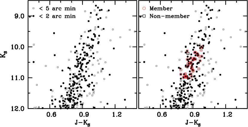
Figure 1.— left: A K_S versus J–K_S color–magnitude diagram, based on 2MASS data (Skrutskie et al. 2006), is shown for the stars inside 2$\arcmin$ (filled black circles) and 5$\arcmin$ (open grey boxes) of the cluster center. right: A plot similar to the left panel but with stars identified as high probability radial velocity members (39 stars) by open red circles and non–members (2 stars) indicated by open black boxes. Note that one target identified as a non–member (2MASS 17023847–2618509) exhibits a double–lined spectrum with one star at a radial velocity consistent with cluster membership and the second star at much lower velocity.

Using the 2MASS astrometry and the Michigan/Magellan Fiber System (M2FS; Mateo et al. 2012) mounted on the Magellan–Clay 6.5m telescope at Las Campanas Observatory, we were able to deploy 47 fibers on one plug plate (41 stars/6 sky). The M2FS fiber system and MSpec spectrograph were configured using the high resolution “Bulge$\_$GC1” setup described in Johnson et al. (2015), which produces cross–dispersed spectra spanning approximately 6120–6720 Å. The 1.2$\arcsec$ fibers and 125$\mu$m slit provided a resolving power of R$\equiv$$\lambda$/$\Delta$$\lambda$$\approx$27,000. The spectra were obtained from a single set of 3$\times$1800 sec exposures on 2014 June 2 under good seeing conditions (FWHM$\approx$0.5$\arcsec$), and this data set yielded 39/41 (95$\%$) stars with radial velocities consistent with cluster membership (see Section 4 for more details). The radial velocity member and non–member stars are identified on the color–magnitude diagram presented in Figure 1.

2.2. Data Reduction

The data reduction process followed the same procedure outlined in Johnson et al. (2015; see their Section 2.3). To briefly summarize, the individual amplifier images (four per CCD) of each exposure were bias subtracted and trimmed separately using the IRAF task ccdproc. Each set of four images was then rotated and translated into the proper orientation and then combined using the IRAF tasks imtranspose and imjoin. The multi–fiber reduction tasks such as aperture identification and tracing, scattered light removal, flat–field correction, ThAr wavelength calibration, cosmic–ray removal, and spectrum extraction, were carried out using repeated calls of the IRAF task dohydra. The final reduction tasks including sky subtraction, continuum fitting, spectrum combination, and telluric removal were accomplished using the IRAF tasks skysub, continuum, scombine, and telluric. The final combined spectra yielded S/N of about 30–50 per resolution element.

3. DATA ANALYSIS

3.1. Model Atmospheres

Due to the presence of significant differential reddening across the cluster (e.g., see Alonso–García et al. 2012; their Figure 13), we determined the model atmosphere parameters effective temperature (T_eff), surface gravity (log(g)), metallicity ([Fe/H]), and microturbulence ($\xi$_mic.) using purely spectroscopic methods. We performed an iterative process that solved for all four model atmosphere parameters simultaneously. Specifically, the effective temperatures were derived by removing trends in log $\epsilon$(Fe I) as a function of excitation potential, the surface gravities were determined by forcing ionization equilibrium between log $\epsilon$(Fe I) and log $\epsilon$(Fe II), and the microturbulences were determined by removing trends between log $\epsilon$(Fe I) and reduced equivalent width (EW). The model atmosphere metallicity was set equal to the average [Fe/H] value determined from each iteration. Since most stars in our sample have [$\alpha$/Fe]$\approx$$+$0.3, as measured from the average of our derived [Mg/Fe], [Si/Fe], and [Ca/Fe] abundances (see Section 5), we interpolated within the available grid of $\alpha$–rich ATLAS9 model atmospheres provided by Castelli & Kurucz (2004). However, the most metal–rich star in our sample (2MASS 17024453$-$2616377) has [$\alpha$/Fe]$\approx$0 so we used the scaled–solar grid for this case. The final adopted model atmosphere parameters are provided in Table 1.

We note that the model atmosphere parameters adopted for this project do not include corrections due to possible departures from local thermodynamic equilibrium (LTE). However, the expected effects on T_eff, log(g), and $\xi$_mic. derived using a spectroscopic analysis and 1D LTE compared to 1D non–LTE are predicted to be $\lesssim$50 K, $\lesssim$0.10 (cgs), and $\lesssim$0.10 km s^-1, respectively, for the parameter space spanned here (Lind et al. 2012). These differences are comparable to the internal precision of our measurements. A similar but possibly relevant issue related to differences in [Fe/H] derived from 1D LTE analyses of RGB, as opposed to AGB, stars has been noted by Ivans et al. (2001; NGC 5904), Lapenna et al. (2014; NGC 104), and Mucciarelli et al. (2015; NGC 3201). These authors found that the derived [Fe I/H] abundances were $\sim$0.10–0.15 dex lower than the [Fe II/H] abundances for AGB, but not RGB, stars when the model atmosphere parameters were determined via spectroscopic methods. Thus, mixing RGB and AGB stars in the same sample could produce an artificial metallicity spread. Unfortunately, the large differential reddening and poor color separation of RGB and AGB stars in Figure 1 makes the assignment of our target stars to either evolutionary state difficult. However, the short evolutionary time scale of AGB stars at the luminosity level reached by our observations suggests a large fraction of the targets are likely first ascent red giants. Additional evidence supporting the detection of a true metallicity spread is provided in Section 5.

3.2. Abundance Analysis

3.2.1 Equivalent Width Measurements

The abundances for all elements were derived using the abfind and synth drivers of the LTE line analysis code MOOG (Sneden 1973; 2014 version). The [Fe/H], [Si/Fe], [Ca/Fe], [Cr/Fe], and [Ni/Fe] abundance ratios were determined using EW measurements made with the semi–automated Gaussian profile fitting code developed for Johnson et al. (2014). In general, we avoided measuring lines that were heavily blended, located near strong telluric features, or that had log(EW/$\lambda$)$\gtrsim$–4.5.

The line selection, atomic transition parameters, and adopted solar abundances are included in Table 2. The log(gf) values were determined through an inverse solar analysis by measuring the EWs of the lines from Table 2 in a daylight solar spectrum taken with the same M2FS configuration as the NGC 6273 data. However, in order to test for possible analysis differences between dwarf and giant stars, we also measured the same lines in the Arcturus atlas (Hinkle et al. 2000). We adopted the model atmosphere parameters given in Ramírez & Allende Prieto (2011) and recovered similar abundances, including the systematic offset of [Fe II/H]–[Fe I/H]$\approx$0.10 dex. Therefore, we increased the solar–based Fe II log(gf) values by 0.10 dex to satisfy ionization equilibrium, and these changes are reflected in Table 2. The final abundances of [Fe/H], [Si/Fe], [Ca/Fe], [Cr/Fe], and [Ni/Fe] are provided in Tables 3a–3b.

3.2.2 Spectrum Synthesis Measurements

The abundances of [Na/Fe], [Mg/Fe], [Al/Fe], [La/Fe], and [Eu/Fe] were measured via spectrum synthesis rather than EW analyses because these elements provide only a small number of often blended lines in the 6120–6720 Å window used here. Additionally, the Mg line profiles near 6318 Å can be affected by a broad Ca autoionization feature, and those of La and Eu are often broadened due to isotopic splitting and/or hyperfine structure. Although the Na, Mg, and Al log(gf) values were determined using a similar procedure described in Section 3.2.1, we adopted the line lists and solar abundances of Lawler et al. (2001a,b) for La and Eu. We also adopted the Solar System isotopic ratio of 47.8$\%$ for ¹⁵¹Eu and 52.2$\%$ for ¹⁵³Eu. Contamination by CN was accounted for in our syntheses by including in our line list the recently updated ¹²C¹⁴N and ¹³C¹⁴N line lists from Sneden et al. (2014). For all stars we set [C/Fe]=–0.3, ¹²C/¹³C=4, and estimated [O/Fe] based on the [Na/Fe] abundances. In particular, the [O/Fe] abundances were estimated from a fit to the [O/Fe]–[Na/Fe] relation provided by Carretta et al. (2009c; their Figure 6) for several Galactic globular clusters. The [N/Fe] abundance was adjusted as a free parameter to provide the best fit to nearby CN features. The final abundances of [Na/Fe], [Mg/Fe], [Al/Fe], [La/Fe], and [Eu/Fe] are provided in Tables 3a–3b.

3.2.3 Internal Abundance Uncertainties

The primary source of error for internal measurement precision comes from uncertainties in the model atmosphere parameter determinations, with additional contributions from line blending, continuum placement, atomic parameters, and visual profile fitting uncertainty. The latter contributions are typically minor for reasonably high resolution and high S/N data, and we have estimated this (largely random) contribution by using the error of the mean for all species analyzed here. On average, the abundance uncertainty on [X/H] ratios from measurement errors alone ranges from $\sim$0.02–0.05 dex.

For the former error source, we estimate that the internal uncertainty for T_eff, log(g), [M/H], and $\xi$_mic. when constrained by spectroscopic methods is approximately 50 K, 0.10 cgs, 0.07 dex, and 0.10 km s^-1, respectively. The T_eff and $\xi$_mic. estimates are derived from the scatter observed when fitting a linear function through plots of log $\epsilon$(Fe I) versus excitation potential (for T_eff) and reduced equivalent width (for $\xi$_mic.). The uncertainty for surface gravity is estimated from the scatter in derived log(g) shown in Table 1 for stars within $\sim$100 K and with similar [Fe/H]. The model atmosphere metallicity uncertainty is estimated from the measurement uncertainty of [Fe I/H] and [Fe II/H]. The total internal uncertainty for each element was calculated by adding in quadrature the measurement error and the change in abundance when each model atmosphere parameter was varied individually. Note that for element ratios normalized by [Fe/H], the change in [Fe I/H] or [Fe II/H] was calculated simultaneously. This procedure ensures that the $\Delta$[X/Fe] uncertainties provided in Tables 3a–3b account for situations in which Fe and the element in question exhibit the same sign of variability when a given model atmosphere parameter is changed.

4. RADIAL VELOCITY MEASUREMENTS AND CLUSTER MEMBERSHIP

Radial velocities were determined using the fxcor task in IRAF to cross correlate against the spectrum of Arcturus (Hinkle et al. 2000). Heliocentric corrections were determined using the IRAF task rvcor. The spectral range from 6120–6275 Å was used for cross correlation, avoiding strong telluric absorption features at wavelengths longer than 6275 Å. The Arcturus spectrum was convolved with a Gaussian profile and rebinned to match the resolution and sampling of the observed spectra. For the M2FS data, this spectral range is split across two orders, giving two independent measures of the radial velocity for each star and for each exposure. The three exposures were measured individually, giving a total of six measurements for each star. The radial velocity dispersions provided in Tables 1 and 4 are the standard deviation of the six measurements.

Although we were only able to derive abundances for 18/41 target stars, we measured radial velocities for all 41 RGB stars. A histogram of our results is shown in Figure 2, and indicates that 39/41 (95$\%$) targets exhibit radial velocities consistent with cluster membership. Table 4 lists the coordinates, 2MASS photometry, and radial velocities for all observed stars not listed in Table 1. We note that one star (2MASS 17023847–2618509) exhibits a double–lined spectrum with one component yielding a velocity consistent with cluster membership and the other component having a velocity inconsistent with cluster membership. The remaining non–member star (2MASS 17024093–2620182) was determined to have [Fe/H]=–0.14, and is thus ruled out as a cluster member based on both kinematics and chemical composition.

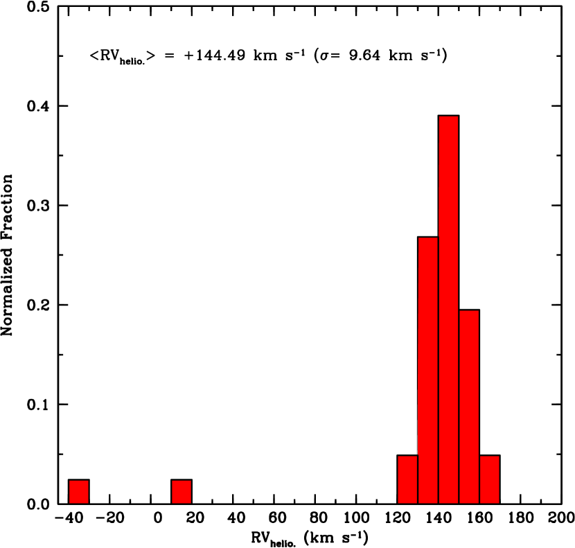
Figure 2.— A histogram showing the distribution of heliocentric radial velocity (RV_helio.) values measured for the stars shown in Figure 1. The data are sampled with 10 km s^-1 bins.

For the stars that do exhibit velocities consistent with cluster membership, we find an average heliocentric radial velocity of $+$144.49 km s^-1 and a dispersion of 9.64 km s^-1. Our derived cluster velocity is larger than the $+$135 km s^-1 value given in Harris (1996; 2010 version), and is also $\sim$20 km s^-1 larger than the $+$121 km s^-1 ($\sigma$=10.6 km s^-1) value provided by Webbink (1981). Additional literature systemic velocities range from $+$120 km s^-1 to $+$147 km s^-1, but there is general agreement that the internal dispersion is $\sim$10 km s^-1 (Zinn & West 1984; Hesser et al. 1986; Rutledge et al. 1997). It is possible that the large range in derived cluster velocities stems from Galactic bulge field star contamination, which can be significant if observations extend beyond a few arc minutes from the cluster core.

Although NGC 6273 lies near the crowded Galactic bulge (l=–3.1,b=$+$9.4), we do not believe a significant fraction of the stars residing near the cluster’s average radial velocity are contaminating bulge field stars. First, the average Galactocentric radial velocity of bulge field stars near l=–3.1 should be approximately –50 km s^-1 with a dispersion of about 80–100 km s^-1 (e.g., Kunder et al. 2012; Ness et al. 2013a; Zoccali et al. 2014). The expected bulge field velocities are in stark contrast to the average Galactocentric velocity of our claimed cluster members at $+$142.02 km s^-1 ($\sigma$=9.64 km s^-1). Second, the Galactic bulge metallicity distribution function cuts off considerably at [Fe/H]$\lesssim$–1 (e.g., Zoccali et al. 2008; Bensby et al. 2013; Johnson et al. 2013; Ness et al. 2013b), and as will be discussed in Section 5.1 the [Fe/H] range of our claimed cluster members spans –1.80 to –1.30. Therefore, finding bulge field stars with [Fe/H]$\sim$–1.5, a high positive velocity, and projected near NGC 6273 should be an extremely rare event.

5. ABUNDANCE RESULTS

5.1. Evidence Supporting a Metallicity Spread

Previous analyses of NGC 6273 have hinted that the cluster may possess an intrinsic metallicity dispersion, as evidenced by a potentially broadened RGB (e.g., Harris et al. 1976; Piotto et al. 1999) and spread in the near–infrared Ca II triplet equivalent width measurements by Rutledge et al. (1997). As mentioned in Section 1, NGC 6273 even shares several observational characteristics (e.g., blue HB; elliptical morphology) with the chemically diverse $\omega$ Cen. However, further interpretation linking these results to an intrinsic metallicity spread have been hindered by the cluster’s significant differential reddening and location near the crowded, and largely metal–rich, Galactic bulge.

The data presented here provide the first detailed high resolution spectroscopic analysis of cluster RGB members, and we find several lines of evidence supporting the presence of an intrinsic metallicity dispersion within NGC 6273. In Figure 3 we show binned metallicity distribution functions for NGC 6273, three monometallic clusters analyzed with M2FS data from the same observing run (NGC 104, NGC 6266, and NGC 6333), and four iron–complex clusters from the literature with confirmed metallicity spreads ($\omega$ Cen, M 2, M 22, and NGC 5286). The three monometallic clusters have [Fe/H] dispersions and interquartile ranges (IQR) of approximately 0.07 and 0.10 dex, respectively. However, using the same instrument and setup, we find NGC 6273 to have $\sigma$_[Fe/H]=0.16 dex and IQR_[Fe/H]=0.25 dex. The larger [Fe/H] dispersion and IQR for NGC 6273 is more in–line with observations of the iron–complex clusters, which have $\sigma$_[Fe/H]$\geq$0.10 dex and IQR_[Fe/H]$\geq$0.15 dex, respectively, when [Fe/H] is derived from high resolution, high S/N spectra.

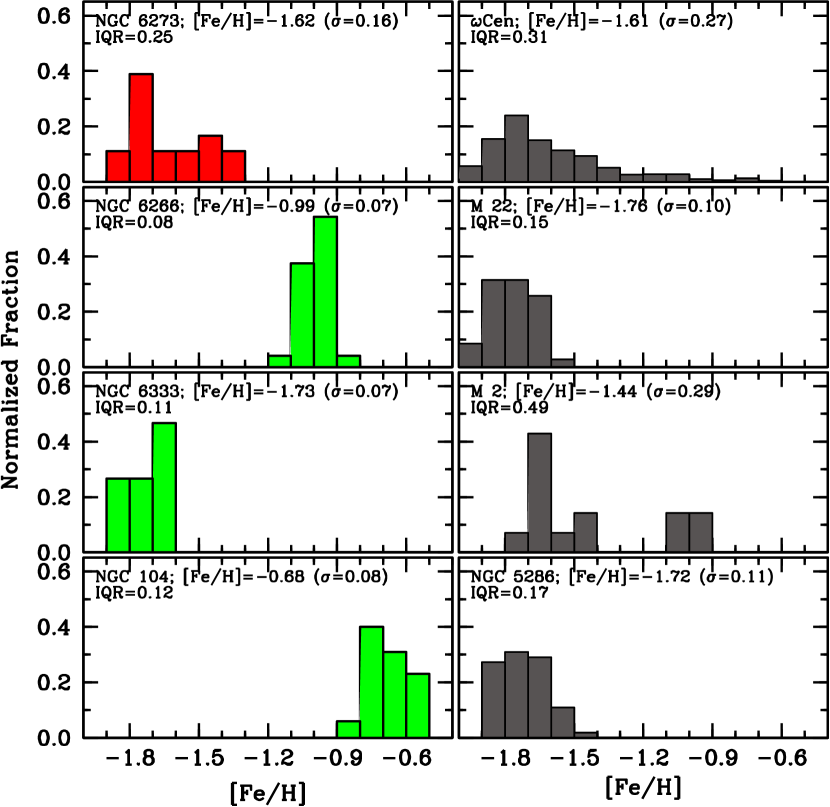
Figure 3.— left: Metallicity distribution functions are shown for NGC 6273 and three other globular clusters observed with M2FS. The results for NGC 6266 and 6333 will be presented in a future publication, but were observed during the same observing run as NGC 6273. The NGC 104 data are available in Johnson et al. (2015). right: Metallicity distribution functions are shown for four additional globular clusters with confirmed metallicity spreads. The data for $\omega$ Cen, M 22, M 2, and NGC 5286 are from: Johnson & Pilachowski (2010), Marino et al. (2011b), Yong et al. (2014), and Marino et al. (2015), respectively. The average [Fe/H] value, dispersion, and interquartile range are provided in all panels, and all data are sampled in 0.1 dex bins.

The overall cluster average of [Fe/H]=–1.62 derived here for NGC 6273 is consistent with previous estimates from photometry (Davidge 2000; Valenti et al. 2007) and calibrated spectroscopic indices (Zinn & West 1984; Kraft & Ivans 2003; Carretta et al. 2009a), which range from [Fe/H]=–1.9 to –1.4. The [Fe/H] distribution shown in Figure 3 exhibits evidence of at least two distinct stellar populations with different metallicities, including a possible third more metal–rich population that has [$\alpha$/Fe]$\approx$0. Therefore, we have separated the stars into three groups, based on each star’s [Fe/H] abundance, which have $\langle$[Fe/H]$\rangle$=–1.75 ($\sigma$=0.04; “metal–poor”), $\langle$[Fe/H]$\rangle$=–1.51 ($\sigma$=0.08; “metal–rich”), and $\langle$[Fe/H]$\rangle$=–1.30 (1 star; “anomalous”). We find that the metal–poor population dominates by number (50$\%$) compared to the metal–rich (44$\%$) and anomalous (6$\%$) groups. However, since we did not target the reddest stars in Figure 1, the fraction of cluster stars with [Fe/H]$\gtrsim$–1.30 may be higher than the 6$\%$ measured here. Although the total sample size is only 18 stars, the average heliocentric radial velocities and dispersions are similar between the metal–poor, metal–rich, and anomalous groups (see Table 5). The similar velocities strongly suggest that all three sub–populations are members of NGC 6273.

Further evidence in support of a metallicity spread can be seen by a visual examination of the spectra. In Figure 4 we compare the M2FS spectra of two stars with similar T_eff and log(g) but that differ in [Fe/H] by more than a factor of two. Note that the line strengths are greater for nearly all transitions in the metal–rich star. The significant increase in EW for La II and Ba II is especially noteworthy. In the context of similar chemical patterns being present in other iron–complex clusters (see Section 6), the observed correlation between [Fe/H] and [La/Fe] in NGC 6273 offers compelling evidence that the [Fe/H] dispersion is real.

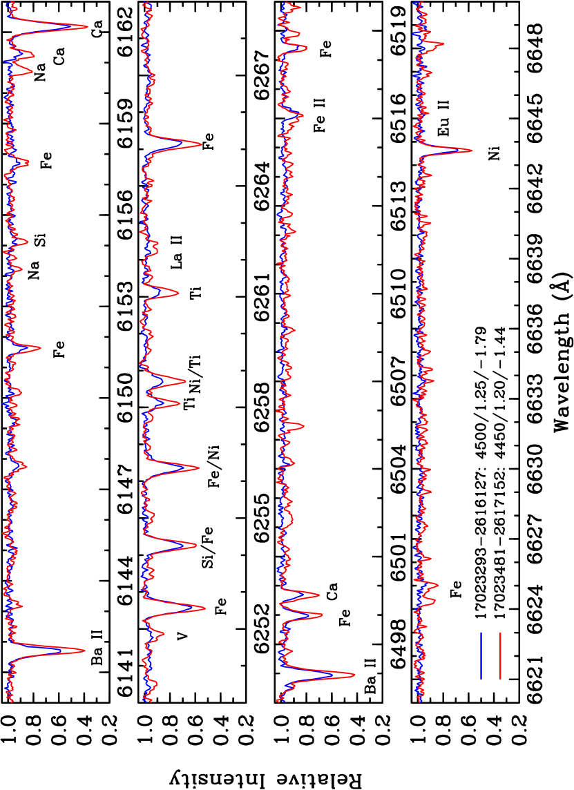
Figure 4.— Sample spectra are shown comparing the line strengths of two stars with similar T_eff and log(g) but different metallicity. The blue spectrum (2MASS 17023293–2616127) is a sample from the metal–poor population and the red spectrum (2MASS 17023480–2617152) is a sample from the metal–rich population.

A similar argument is made by examining the location of stars on the color–magnitude diagram when separated by [Fe/H]. Figure 5 shows that, even in a near–infrared color–magnitude diagram that is not corrected for differential reddening, for a given luminosity level the more metal–poor stars tend to be bluer than the more metal–rich stars. Furthermore, the RGB color dispersion may be largely explained by the presence of differential reddening and a $\sim$0.5 dex spread in [Fe/H]. A similar conclusion is reached when examining the dereddened optical color–magnitude diagram from Piotto et al. (1999; 2002) shown in Figure 6. We were able to match one star from each spectroscopically defined sub–population to the original Hubble Space Telescope images from Piotto et al. (1999; 2002), and again we find that the stars are distributed as one would expect if the RGB color dispersion was at least partially driven by a metallicity spread. Interestingly, both Figures 5 and 6 show evidence of stars residing at even redder colors than were observed here. While these may belong to the Galactic bulge field population, they are found projected near the dense cluster core. If some fraction of these presumably more metal–rich stars are cluster members, then the metallicity spread would exceed 0.5 dex. Such a large [Fe/H] spread would make NGC 6273 more similar to $\omega$ Cen and M 2 than the less extreme iron–complex clusters.

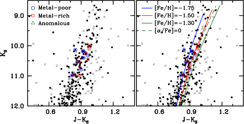
Figure 5.— Color–magnitude diagrams similar to Figure 1 are shown but with the observed high probability cluster members designated by metallicity. The metal–poor ([Fe/H]$\approx$–1.75), metal–rich ([Fe/H]$\approx$–1.50), and “anomalous” ([Fe/H]$\approx$–1.30) populations are designated with the open blue circles, open red boxes, and open green triangles, respectively. Dartmouth stellar isochrones (Dotter et al. 2008) with ages of 12 Gyr, [Fe/H]=–1.75, –1.50, and –1.30, and [$\alpha$/Fe]=$+$0.20 are overlaid as blue, red, and green solid lines, respectively. We assumed a distance of 9 kpc (Piotto et al. 1999) and E(B-V)=0.30, which provided the best agreement between photometric and spectroscopic temperatures (see Section 5.1). A similar isochrone with [Fe/H]=–1.30 and [$\alpha$/Fe]=0, which matches more closely to the abundance pattern of the anomalous star, is plotted as a dashed green line.

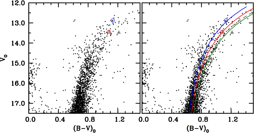
Figure 6.— Hubble Space Telescope (HST) optical color–magnitude diagrams are shown for the RGB regions of NGC 6273. The data are from Piotto et al. (1999; 2002) and have been dereddened following the prescriptions outlined in the original papers. The right panel shows the same color–magnitude diagrams but with the isochrones from Figure 5 over plotted. The open symbols are the same as in Figure 5, and represent three stars (2MASS 17023868–2616516, 17024016–2616096, and 17024453–2616377) we were able to match from our sample onto the Piotto et al. (1999) HST images.

5.2. Light Odd–Z and $\alpha$ Element Abundances

In Figure 7 we present a box plot of the [X/Fe] ratios for all elements analyzed here. For the elements with Z$\leq$20, [Mg/Fe] ($\sigma$=0.12 dex), [Si/Fe] ($\sigma$=0.11 dex), and [Ca/Fe] ($\sigma$=0.09 dex) have the smallest abundance dispersions. From these data and the abundance uncertainties listed in Tables 3a–3b, we conclude that a dispersion of $\sim$0.10 dex is the limit separating elements with and without significant abundance spreads. Therefore, among the light elements both [Na/Fe] ($\sigma$=0.18 dex) and [Al/Fe] ($\sigma$=0.31 dex) exhibit substantial star–to–star scatter. However, the abundances of [Na/Fe] and [Al/Fe] are correlated (see Figure 8), and [Al/Fe] even shows some evidence of a bimodal distribution. In particular, we do not find any stars with $+$0.45$\lesssim$[Al/Fe]$\lesssim$$+$0.75, and the gap appears to be present in both the metal–poor and metal–rich groups. We note that a similar feature has been observed in other clusters, such as $\omega$ Cen (Norris & Da Costa 1995; Johnson et al. 2008; Johnson & Pilachowski 2010) and NGC 2808 (Carretta 2014), as well. Figure 8 shows some (weak) evidence in support of a Mg–Al anti–correlation, which is expected if Al production is driven by the MgAl proton–capture cycle. However, more data are needed to confirm this result.

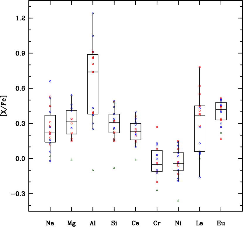
Figure 7.— A box plot illustrating the [X/Fe] ratios of all elements measured here. The target stars are designated using the same colors and symbols as in Figure 5. For each element column the three horizontal lines indicate the first quartile, median, and third quartile values for all stars. The vertical lines indicate the full range of [X/Fe] values, excluding outliers ($>$1.5$\times$ the interquartile range).

Although both the metal–poor and metal–rich populations independently show a Na–Al correlation, Figures 7–8 and Table 5 indicate that the dispersion is not equivalent between the two main sub–populations. The metal–poor and metal–rich groups have similar average [Na/Fe] and [Al/Fe] abundances, but the star–to–star dispersion is larger for the metal–poor group. However, the dispersion for [Mg/Fe], [Si/Fe], and [Ca/Fe] is essentially identical between the metal–poor and metal–rich groups. The metal–poor stars have slightly higher [Mg/Fe], [Si/Fe], and [Ca/Fe] abundances than the metal–rich stars, but both populations are $\alpha$–enhanced ([$\alpha$/Fe]$\approx$$+$0.30). In fact, the average difference in overall [$\alpha$/Fe] between the two populations is only 0.06 dex.

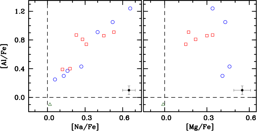
Figure 8.— left: A plot of [Al/Fe] versus [Na/Fe] is shown for NGC 6273 stars. Similar to Figure 5, the metal–poor, metal–rich, and “anomalous” RGB stars are designated as open blue circles, open red boxes, and open green triangles. Note that both main populations exhibit the well–known Na–Al correlation characteristic of high–temperature proton–capture nucleosynthesis, and also exhibit a noticeable gap between $+$0.45$\lesssim$[Al/Fe]$\lesssim$$+$0.75. The dashed lines in both panels represent the solar abundance ratios. right: A plot of [Al/Fe] versus [Mg/Fe] for the same stars as in the left panel. The sample size of stars within each sub–population is too small to conclude whether or not a Mg–Al anti–correlation is present. Typical error bars are shown (black symbol) in the bottom right corner of each panel.

The single anomalous star in our sample is the most metal–rich ([Fe/H]=–1.30) and also has a peculiar composition. Unlike the metal–poor and metal–rich groups, the anomalous star has [X/Fe]$\sim$0 for all elements with Z$\leq$20 measured here. As can be seen in Figure 7, the anomalous star’s abundance pattern is an outlier for all light elements except [Na/Fe]. Although it is not unusual for a globular cluster to host stars with [Na/Fe]$\sim$0 and/or [Al/Fe]$\sim$0, very few clusters have [$\alpha$/Fe]$\sim$0 (e.g., see Gratton et al. 2004; their Figure 4). Interestingly, the few clusters confirmed to have low mean [$\alpha$/Fe] abundances, such as Rup 106 and Pal 12 (Brown et al. 1997; Cohen 2004), may not be native to the Milky Way and are proposed to be relics of captured systems (e.g., Lin & Richer 1992; Law & Majewski 2010). The anomalous star’s radial velocity and location on the color–magnitude diagram support the notion that it is a cluster member. However, one study cannot definitively constrain whether the anomalous star was formed in situ with the metal–poor and/or metal–rich groups, or was captured from another system or stream.

5.3. Fe–Peak Element Abundances

As is evident from Figure 7, both Cr ($\langle$[Cr/Fe]$\rangle$=–0.01 dex; $\sigma$=0.13 dex) and Ni ($\langle$[Ni/Fe]$\rangle$=–0.02 dex; $\sigma$=0.10 dex) closely track Fe and have approximately the same average abundance. Similarly, both the metal–poor and metal–rich sub–populations have equivalent [Cr/Fe] and [Ni/Fe] abundances and dispersions (see Table 5). The relatively small star–to–star scatter and [X/Fe]$\approx$0 pattern for the Fe–peak elements is typical of most Galactic globular clusters (e.g., see review by Gratton et al. 2004).

In addition to having [$\alpha$/Fe]$\sim$0, the anomalous star exhibits a very peculiar Fe–peak abundance pattern with [Cr/Fe]=–0.27 and [Ni/Fe]=–0.36. The factor of two depletion for Cr and Ni relative to Fe is particularly puzzling because both elements typically follow similar production patterns with Fe. We are only aware of a few cases in which the even–Z Fe–peak elements have a significant depletion relative to Fe, including the aforementioned Rup 106 and Pal 12 (Brown et al. 1997; Cohen 2004), Terzan 7 (Tautvaišienė et al. 2004; Sbordone et al. 2005), and the open cluster M 11 (Gonzalez & Wallerstein 2000). There is also a small but growing number of individual stars with similar even–Z element deficiencies such as CS 22169–035 ([Fe/H]=–3.04; Cayrel et al. 2004), Car–612 ([Fe/H]=–1.30; Venn et al. 2012), HE 1207–3108 ([Fe/H]=–2.70; Yong et al. 2013), and the modestly metal–poor field stars HD 193901 and HD 194598 ([Fe/H]$\approx$–1.15; Jehin et al. 1999; Gratton et al. 2003; Jonsell et al. 2005). Several of the systems observed to have low [Cr,Ni/Fe] are associated with the captured Sagittarius dwarf spheroidal system, and nearly all of the low [Ni/Fe] objects also have low [$\alpha$/Fe]. The similar abundance pattern of these objects with the anomalous star in NGC 6273 suggests that, assuming the anomalous star is a cluster member, the final stage of star formation in NGC 6273 may have proceeded under conditions not experienced by most globular clusters (e.g., unusual initial mass function; long time delay) or that NGC 6273 may have accreted stars or gas from another system.

5.4. Neutron–Capture Element Abundances

We find that the dispersion for [La/Fe] ($\sigma$=0.25 dex) is significantly larger than for [Eu/Fe] ($\sigma$=0.11 dex), and Figure 7 indicates that the [La/Fe] dispersion is only exceeded by that of [Al/Fe]. However, Figure 9 shows that [La/Fe] is not well correlated with either [Na/Fe] or [Al/Fe], which suggests that the two element groups are produced by different sources. Interestingly, [La/Fe] is strongly correlated with [Fe/H] and increases steadily from [La/Fe]$\sim$–0.10 in the most metal–poor stars to [La/Fe]$\sim$$+$0.50 in the most metal–rich stars (except for the anomalous star). In contrast, the Eu abundance remains relatively constant at [Eu/Fe]$\approx$$+$0.40 (see Figure 10). The strong rise in [La/Fe] as a function of increasing [Fe/H], coupled with the enhanced and nearly constant [Eu/Fe] abundance, is a trait that is common to many iron–complex globular clusters (see Section 6).

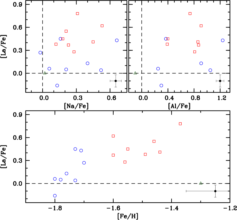
Figure 9.— The top two panels are similar to Figure 8 except [La/Fe] is plotted as a function of [Na/Fe] (left) and [Al/Fe] (right). The bottom panel shows [La/Fe] plotted as a function of [Fe/H]. Note the strong rise in [La/Fe] as a function of increasing [Fe/H]. A typical error bar is shown in the bottom right corner of each panel.

A comparison of the [La/Fe], [Eu/Fe], and [La/Eu] ratios as a function of sub–population, [Fe/H], and [La/H] is shown in Figures 9–10 and Table 5. The [La/Fe] dispersion is marginally larger for the metal–poor population, and in fact [La/Fe] rises as a function of [Fe/H] approximately twice as fast in the metal–poor group as the metal–rich group. However, the anomalous star deviates from the overall cluster trend and has [La/Fe]=0, despite being the most metal–rich star. Since [Eu/Fe] is nearly constant across all three sub–populations, the change in [La/Eu], which is a measure of the relative contributions from the s–process and r–process and is largely insensitive to model atmosphere uncertainties, with metallicity follows the [La/Fe] trend. As can be seen in Figure 10, [La/Eu] increases from [La/Eu]$\sim$–0.60 to [La/Eu]$\sim$0.00 in the metal–poor population. The [La/Eu] ratio either remains constant at [La/Eu]$\sim$0.00 or slowly increases for the metal–rich population. The anomalous star has [La/Eu]$\sim$–0.20, which is more in–line with some of the more metal–poor stars.

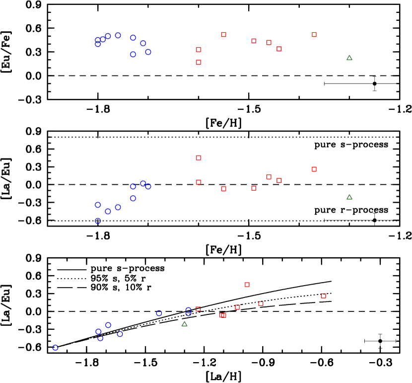
Figure 10.— The top and middle panels plot [Eu/Fe] and [La/Eu] as a function of [Fe/H]. The [La/Eu] ratio is a measure of the relative contributions from the s–process and r–process. The increasing [La/Eu] ratio with increasing metallicity is a characteristic of s–process enrichment. Following McWilliam et al. (2013), the bottom panel shows [La/Eu] as a function of [La/H]. The solid black line illustrates the expected enrichment profile when pure s–process material is added to a pure r–process composition. The dotted and long dashed lines indicate the expected profiles for 95$\%$(s)/5$\%$(r) and 90$\%$(s)/10$\%$(r) mixtures added to a pure r–process composition. The remaining colors and symbols are the same as those in Figure 5, and the pure r–process and s–process values are from Kappeler et al. (1989) and Bisterzo et al. (2010), respectively.

The peculiar shape of the [La/Eu] versus [Fe/H] distribution warrants further investigation. The low [La/Eu] ratio for the most metal–poor stars in NGC 6273 is a characteristic shared with most globular clusters, and is consistent with a pure r–process distribution. Therefore, the rise in [La/Fe], but not [Eu/Fe], with increasing [Fe/H] suggests the [La/Eu] increase is driven primarily by s–process production. Following McWilliam et al. (2013) and adopting [La/Eu]=–0.60 (Kappeler et al. 1989) and $+$0.80 (Bisterzo et al. 2010) as the pure r–process and s–process ratios, in Figure 10 we plot [La/Eu] as a function of [La/H]. We also include three simple dilution models that mix pure s–process, 95$\%$ s–process, and 90$\%$ s–process material with an initial pure r–process composition. As noted by McWilliam et al. (2013), this plot removes the production degeneracy of [Fe/H] since Fe can be produced in both Type II and Type Ia supernovae. The data and models in Figure 10 suggest that the metal–poor population may be well–fit by assuming the dispersion in [La/Eu] is driven by mixing pure s–process material with the initial (primordial?) pure r–process composition. Interestingly, the more metal–rich stars are better fit by a model that assumes a 5–10$\%$ contribution from the r–process, which is perhaps an indication that the stars producing Fe for the metal–rich generation also synthesized some Eu. The anomalous star is again peculiar in composition and may be consistent with a model that assumes a $>$10$\%$ contribution from the r–process.

6. COMPARISON WITH OTHER “IRON–COMPLEX” GLOBULAR CLUSTERS

As mentioned in Section 1, the peculiar metallicity spread and heavy element abundance patterns exhibited by NGC 6273 separate the cluster from the bulk of the Galaxy’s globular cluster population. Instead, NGC 6273 may belong to a growing class of iron–complex clusters that still exhibit the large star–to–star light element abundance dispersions that define a system as a globular cluster, but that also have $\sigma$_[Fe/H]$\gtrsim$0.10, IQR_[Fe/H]$\gtrsim$0.15, and large s–process abundance spreads that are correlated with [Fe/H]. A comparison between NGC 6273 and the iron–complex clusters $\omega$ Cen, M 22, M 2, M54$+$Sagittarius dwarf spheroidal galaxy, NGC 1851, and NGC 5286 are summarized in Figures 11–15. Even though all of these systems exhibit significant [Fe/H] and heavy element spreads and are included for context, we will primarily focus on comparing NGC 6273 with $\omega$ Cen, M 22, M 2, and NGC 5286. These four clusters appear to share the closest chemical composition and formation history with NGC 6273.

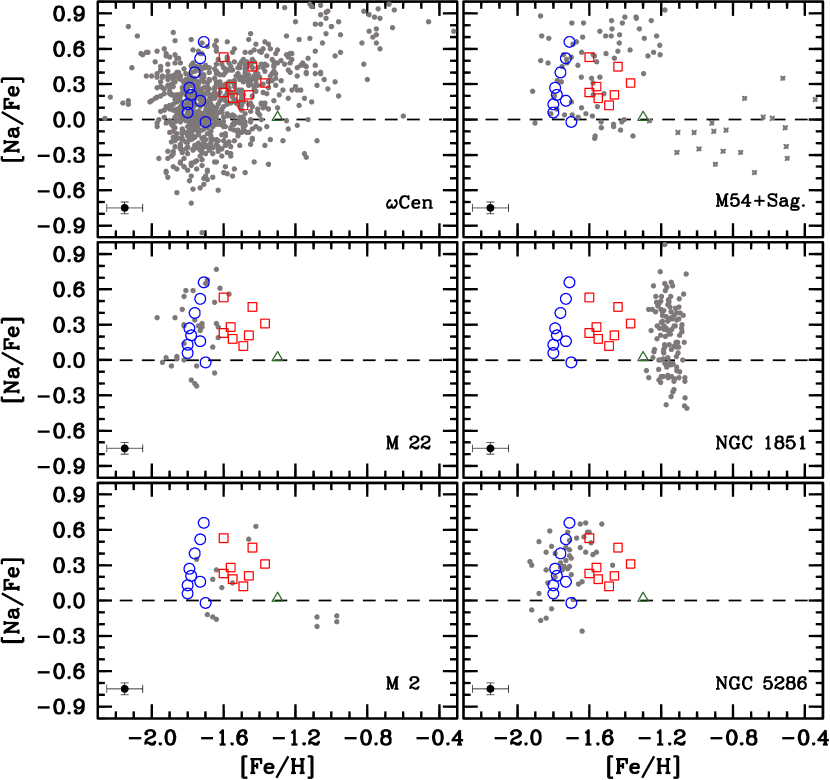
Figure 11.— [Na/Fe] abundances are plotted as a function of [Fe/H] for NGC 6273 (open blue circles, red boxes, and green triangles as in Figure 5) and six additional iron–complex globular clusters. The data for $\omega$ Cen, M 22, M 2, M54 $+$ Sagittarius, NGC 1851, and NGC 5286 are from: Carretta et al. (2010a,b), Johnson & Pilachowski (2010), Carretta et al. (2011), Marino et al. (2011b), Yong et al. (2014), and Marino et al. (2015). The dashed lines indicate the solar abundance ratios.

A comparison of the NGC 6273 [Na/Fe] abundances with the other iron–complex clusters is shown in Figures 11. In general, we find that NGC 6273 shares a similar average [Na/Fe] abundance and star–to–star dispersion with the other clusters. Additionally, Figure 11 indicates that there may be a pattern of decreasing [Na/Fe] dispersion for the more metal–rich populations of NGC 6273, $\omega$ Cen, and possibly NGC 5286. We note that a decrease in [Na/Fe] dispersion with increasing [Fe/H] would fit a global trend observed in monometallic globular clusters as well (e.g., Carretta et al. 2009b, their Figure 3; Johnson & Pilachowski 2010, their Figure 15). A decrease in both the maximum [Al/Fe] abundance and dispersion for the more metal–rich populations is clearly seen in both NGC 6273 and $\omega$ Cen (Figure 12), and also matches trends observed in monometallic clusters (e.g., Carretta et al. 2009b; O’Connell et al. 2011; Cordero et al. 2014, 2015). The prominent bimodal [Al/Fe] distribution of NGC 6273 is also clearly seen in $\omega$ Cen, M54$+$Sagittarius, and possibly M 2. Plotting [Al/Fe] as a function of [Na/Fe] in Figure 13 further reveals that most of the iron–complex clusters likely host discreet light element populations and share a common Na–Al correlation slope. Since most of the clusters in Figure 13 have approximately the same metallicity (see also Figure 3), the common Na–Al correlation slope may be an indication that a similar mass range of sources polluted each cluster.

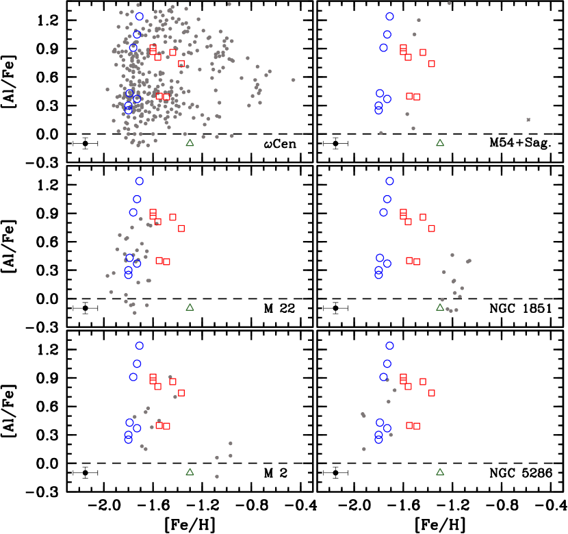
Figure 12.— A similar plot to Figure 11 showing [Al/Fe] as a function of [Fe/H].

The discreet nature of the Na–Al correlation is not surprising given that both normal and iron–complex clusters exhibit well–separated photometric sequences when observed with filters sensitive to light element abundances (e.g., Piotto et al. 2015). However, since the light element (anti–)correlations are present in both normal clusters and in the various populations hosted by most iron–complex clusters, it is clear that the process which produces a metallicity and neutron–capture abundance spread is independent of light element production.

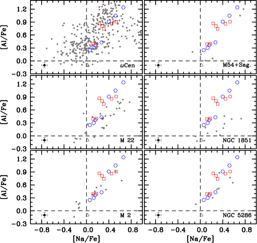
Figure 13.— A similar plot to Figure 11 showing [Al/Fe] as a function of [Na/Fe].

Although nearly all globular clusters exhibit similar light element abundance patterns, the correlated increase in [La/Fe] with [Fe/H] is perhaps the most unusual and defining characteristic of iron–complex clusters. As can be seen in Figures 14–15, the shape and slope of the [La/Fe] and [La/Eu] distributions are nearly identical for all of the iron–complex clusters (see also Marino et al. 2015). Combining the information from Figures 10 and 15 indicates that in all of the iron–complex clusters included here the increase in [La/Eu] is due to almost pure s–process enrichment. Previous work on iron–complex clusters such as M 2 (Lardo et al. 2013; Yong et al. 2014), M 22 (Marino et al. 2009, 2011b), and NGC 5286 (Marino et al. 2015) suggested that each may be decomposed into at least two populations: a low [La/Eu] metal–poor group and a high [La/Eu] metal–rich group. The data presented in Figures 14–15 support these findings, and Figure 15 in particular suggests that clusters with similar [Fe/H] also differentiate in [La/Eu] at about the same [La/H] abundance. For clusters with [Fe/H]$\sim$–1.7, the increase in [La/Eu] occurs near [La/H]$\sim$–1.6 to –1.4.

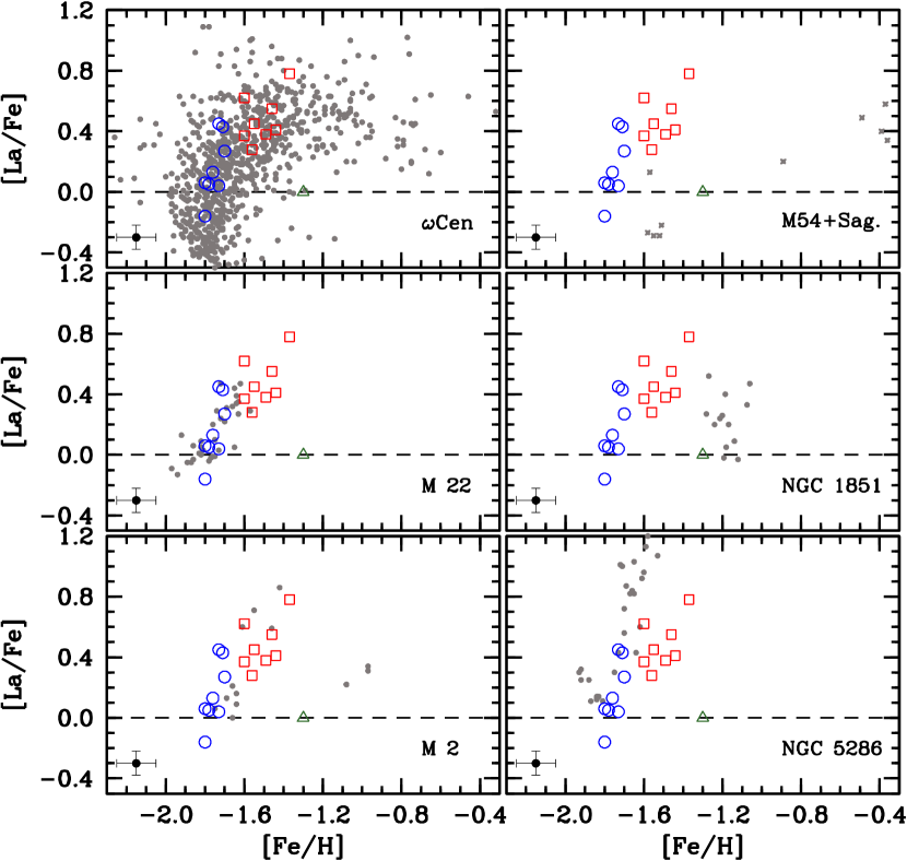
Figure 14.— A similar plot to Figure 11 showing [La/Fe] as a function of [Fe/H]. Additional references for M54 $+$ Sagittarius include Brown et al. (1999), Sbordone et al. (2007), and McWilliam et al. (2013).

The similar heavy element abundance patterns observed for many iron–complex clusters makes it tempting to speculate that all of them formed through the same basic process. However, just as both normal and iron–complex clusters exhibit similar light element abundance variations but can have very different heavy element distributions, the similar s–process abundances of the iron–complex clusters could be a red herring. In other words, different formation mechanisms, timescales, and/or evolution paths may produce clusters with similar composition characteristics. For example, M 22, M 2, and $\omega$ Cen exhibit a similar increase in [La/Eu] over the same [La/H] range, but the s–process production site may not be the same. Roederer et al. (2011) and Yong et al. (2014) find in M 22 and M 2, respectively, that the s–process production may be best fit by pollution from $\gtrsim$3 M_⊙ AGB stars (see also Shingles et al. 2014; Straniero et al. 2014). In contrast, Smith et al. (2000) find in $\omega$ Cen that the s–process production may be best fit by pollution from $\sim$1.5–3 M_⊙ AGB stars. A similar conclusion is reached by Marino et al. (2015) through a comparison of the change in $\frac{\Delta[Ba/Fe]}{\Delta[Fe/H]}$ between M 22, M 2, and NGC 5286. These authors suggest that the larger [Ba/Fe] range found in M 2 and NGC 5286 stars compared to M 22 stars may be due to different classes of polluters enriching the cluster interstellar mediums. Although all iron–complex clusters exhibit similar r–process dominated metal–poor populations, the variable extent of s–process production between clusters may be a sign of different enrichment histories.

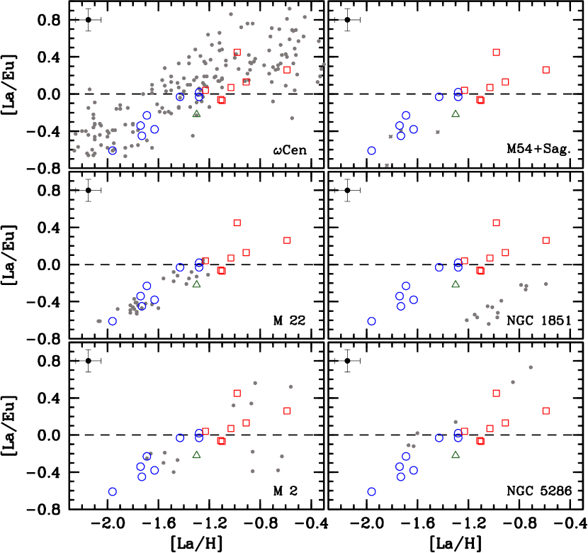
Figure 15.— A similar plot to Figures 10–11 showing [La/Eu] as a function of [La/H].

A key remaining question is whether the s–process–rich populations in iron–complex clusters are predominantly influenced by pollution from low–intermediate mass AGB stars of the r–process dominated group or accretion/mergers from a separate population. Since most present–day monometallic globular clusters do not have significant s–process enhancements, we can speculate that either intracluster pollution or gas accretion from a surrounding system (e.g., dwarf galaxy) are the more likely processes. An interesting coincidence noted by Marino et al. (2015) is that a large fraction of the known iron–complex clusters have approximately the same metallicity ([Fe/H]$\sim$–1.7), and in fact NGC 6273 fits into this pattern. The spatial and kinematic distribution of the iron–complex clusters does not strongly suggest that they originated from a common system. However, understanding the significance, if any, of this observation may be an important component that leads to a better understanding of globular cluster formation.

6.1. The Metal–rich Anomalous Populations

As previously noted, the most metal–rich star in NGC 6273 exhibits a peculiar composition compared to both the metal–poor and metal–rich sub–populations. Interestingly, the iron–complex clusters $\omega$ Cen, M 2, and NGC 5286 also host similar peculiar populations. In all four clusters these “anomalous” stars share the characteristics of being minority populations ($\lesssim$5$\%$) that have higher [Fe/H] than the metal–poor populations yet have lower [La/Eu] ratios than the metal–rich populations. However, the anomalous stars in each cluster are not a universally homogeneous population. For example, the anomalous stars in NGC 6273 and M 2 have low [Na/Fe], [Al/Fe], and [$\alpha$/Fe] ratios, those in $\omega$ Cen have an unusual O–Na correlation, and those in NGC 5286 have low s–process abundances but relatively normal light and $\alpha$–element abundances. The anomalous star in NGC 6273 also has low [Cr/Fe] and [Ni/Fe] abundances, which are characteristics not shared by any other anomalous population.

The origin of these anomalous metal–rich populations may hold additional clues for understanding the formation of complex clusters. Figures 11–15 suggest that the anomalous populations of NGC 6273 and M 2 may share a similar composition with the Sagittarius field star population. Therefore, it is tempting to speculate that the minority population of anomalous stars present in some clusters is the by product of accreting field stars from a progenitor system. Dynamical simulations may be particularly useful for estimating the fraction of field stars that might remain bound to the cluster from accretion during such a scenario (e.g., see Bekki & Yong 2012). From an observational stand point, obtaining composition information for a larger sample of anomalous stars is needed in order to determine if a metallicity spread is present in the anomalous population as well, or if those stars represent a monometallic population. The distinct color–magnitude diagram sequences for the anomalous stars in $\omega$ Cen and M 2 (e.g., Lee et al. 1999; Milone et al. 2015) suggest that they may be a single, coeval population. However, Marino et al. (2015) note that the anomalous stars in NGC 5286 may instead represent a metallicity spread of the metal–poor population.

Since NGC 6273 orbits predominantly near the Galactic bulge and between $\sim$0.5 and 2.5 kpc from the Galactic center (Carollo et al. 2013; Moreno et al. 2014), in Figure 16 we compare the anomalous star’s composition to the metal–poor bulge field stars. We find that the anomalous star has [Na/Fe], [Al/Fe], [La/Fe], and [Eu/Fe] abundances that are consistent with the bulge field star population. However, the anomalous star’s low [$\alpha$/Fe], [Cr/Fe], and [Ni/Fe] abundances do not match the bulge field star pattern. Therefore, we conclude that the anomalous star in NGC 6273 was likely not accreted from the present–day bulge field population.

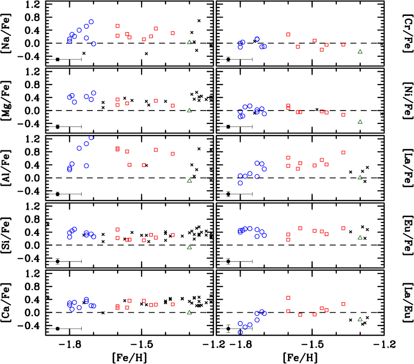
Figure 16.— Plots of all elements measured for NGC 6273 are shown as a function of [Fe/H], and the cluster abundances are compared with those of metal–poor Galactic bulge field stars (black crosses). The cluster symbols are the same as those in Figure 5. The bulge field star data are from: Lecureur et al. (2007), Alves–Brito et al. (2010), McWilliam et al. (2010), Bensby et al. (2011; 2013), Gonzalez et al. (2011), Johnson et al. (2011; 2012; 2013; 2014), and García Pérez et al. (2013). Note that the scale of the ordinate axis is the same for all panels, and that the dashed lines indicate the solar abundance ratios.

7. SUMMARY

Using high resolution spectra obtained with the M2FS instrument on the Magellan–Clay telescope, we have measured radial velocities (41 stars) and chemical compositions (18 stars) for RGB stars in the Galactic globular cluster NGC 6273. Our results indicate that NGC 6273 belongs to a growing class of “iron–complex” clusters that exhibit both a large [Fe/H] dispersion and a correlated increase in [La/Fe] with [Fe/H]. Specifically, we find that NGC 6273 hosts at least 2–3 distinct stellar populations: (1) a metal–poor group with $\langle$[Fe/H]$\rangle$=–1.75 ($\sigma$=0.04) and a spread in [La/Fe], (2) a metal–rich group with $\langle$[Fe/H]$\rangle$=–1.51 ($\sigma$=0.08) and enhanced [La/Eu] ratios, and (3) a possible anomalous group with $\langle$[Fe/H]$\rangle$=–1.30 (1 star) and noticeably lower [X/Fe] ratios for nearly all elements. Despite a moderate sample size, we find that the two main populations are nearly equivalent in number, and that the metal–poor, metal–rich, and anomalous groups constitute 50$\%$, 44$\%$, and 6$\%$ of our sample, respectively. Additionally, the cluster’s broad giant branch may be explained by a combination of significant differential reddening and a spread in [Fe/H] of at least 0.5 dex.

Interestingly, the metal–poor and metal–rich sub–populations independently exhibit the well–known Na–Al correlation, but the dispersion in both [Na/Fe] and [Al/Fe] is larger for the more metal–poor stars. Furthermore, the [Al/Fe] distribution appears to be largely bimodal, and we do not find any stars with $+$0.45$\lesssim$[Al/Fe]$\lesssim$$+$0.75 in either sub–population. However, [Na/Fe] and [Al/Fe] are not correlated with either [Fe/H] or [La/Fe], which suggests that the nucleosynthesis process that creates the Na–Al correlation operates independently from the process that produces the Fe–peak and s–process elements. The metal–poor and metal–rich groups also exhibit similarly enhanced [$\alpha$/Fe] and [Eu/Fe] abundances.

The most unusual composition characteristic of NGC 6273 is the cluster’s correlated increase in [La/Fe] with [Fe/H]. We find that [La/Fe] increases steadily from [La/Fe]$\sim$–0.10 to [La/Fe]$\gtrsim$$+$0.50 between the metal–poor and metal–rich groups. A plot of [La/Eu] versus [La/H] reveals that the increase in La abundance is due to almost pure s–process production, with perhaps a 5–10$\%$ r–process contribution in the metal–rich group. Interestingly, the anomalous star has [La/H] and [La/Eu] abundances that are similar to stars in the metal–poor group.

A comparison of the abundance patterns seen in NGC 6273 with other iron–complex clusters (e.g., $\omega$ Cen, M 2, M 22, and NGC 5286) reveals that many of them share similar light and heavy element composition characteristics. Furthermore, nearly all iron–complex clusters also have [Fe/H]$\sim$–1.7. In addition to NGC 6273, a few clusters such as $\omega$ Cen, M 2, and NGC 5286 also host anomalous metal–rich populations with peculiar abundances. However, the detailed composition for each anomalous population may be unique to each cluster, and may indicate that these stars were originally part of a different system or accreted from a larger progenitor host.

Despite growing evidence that NGC 6273 and other iron–complex clusters are fundamentally different from monometallic clusters, several key questions remain. One of the most fundamental questions is which physical processes are required to produce a cluster with and without a metallicity spread? Furthermore, why do some iron–complex clusters have a unimodal but broadened [Fe/H] distribution and others have discreet populations? Additionally, why do most (or all) metal–poor clusters with [Fe/H] dispersions have strong s–process enrichment? The large [La/Eu] abundances found in iron–complex clusters are not representative of a typical metal–poor field star nor a monometallic globular cluster composition. The nature of the peculiar, metal–rich populations seen only in some iron–complex clusters may hold additional insight regarding cluster formation. Specifically, did these populations form in situ with the other metallicity groups, do they reflect primordial variations, or are they the result of accretion and/or merger events from a separate population? Finally, can more than one formation and/or evolution process produce clusters with similar composition characteristics?

Table 1Stellar Parameters

Star Name	RA (J2000)	DEC (J2000)	J	H	KS	Teff	log(g)	[Fe/H]	$\xi$mic.	RVhelio.	RV Error
(2MASS)	(Degrees)	(Degrees)	(mag.)	(mag.)	(mag.)	(K)	(cgs)	(dex)	(km s-1)	(km s-1)	(km s-1)
Metal–Poor Population
17023158$-$2617259	255.631607	$-$26.290541	11.412	10.726	10.550	4400	0.80	$-$1.80	1.85	158.72	0.24
17023856$-$2617209	255.660695	$-$26.289145	10.980	10.287	10.134	4275	0.60	$-$1.80	1.55	143.95	0.16
17023293$-$2616127	255.637211	$-$26.270214	11.801	11.201	10.988	4500	1.25	$-$1.79	1.90	131.93	0.36
17022785$-$2615555	255.616065	$-$26.265430	11.692	10.941	10.792	4425	0.90	$-$1.78	1.80	144.57	0.19
17024618$-$2615261	255.692427	$-$26.257250	11.284	10.518	10.322	4275	0.65	$-$1.76	1.70	162.46	0.08
17023289$-$2615535	255.637042	$-$26.264864	11.103	10.396	10.181	4300	0.45	$-$1.73	1.60	158.80	0.23
17023509$-$2616406	255.646228	$-$26.277952	11.098	10.385	10.182	4225	0.65	$-$1.73	1.70	145.77	0.19
17023868$-$2616516	255.661183	$-$26.281012	11.323	10.572	10.400	4500	1.15	$-$1.71	1.75	138.02	0.24
17023384$-$2616416	255.641002	$-$26.278240	11.785	11.066	10.952	4525	1.15	$-$1.70	1.60	143.52	0.14
Metal–Rich Population
17024016$-$2616096	255.667344	$-$26.269346	11.416	10.699	10.451	4575	1.55	$-$1.60	1.65	126.39	0.12
17023078$-$2615183	255.628290	$-$26.255096	11.631	10.904	10.737	4600	1.35	$-$1.60	1.90	157.43	0.06
17025121$-$2617230	255.713406	$-$26.289745	11.079	10.280	10.104	4450	1.15	$-$1.56	1.75	134.13	0.37
17024326$-$2617504	255.680281	$-$26.297361	11.864	11.166	10.982	4450	1.20	$-$1.55	1.60	123.37	0.22
17025221$-$2614307	255.717545	$-$26.241865	11.807	11.118	10.972	4400	1.20	$-$1.49	1.45	148.81	0.30
17023424$-$2615437	255.642703	$-$26.262144	10.977	10.215	10.000	4325	1.25	$-$1.46	1.75	153.76	0.07
17023481$-$2617152	255.645044	$-$26.287563	11.415	10.681	10.535	4450	1.20	$-$1.44	1.80	148.11	0.20
17023301$-$2615360	255.637556	$-$26.260017	11.211	10.482	10.264	4400	1.65	$-$1.37	1.90	141.00	0.25
Anomalous Population
17024453$-$2616377	255.685573	$-$26.277155	11.288	10.507	10.307	4350	1.10	$-$1.30	1.60	143.06	0.21

Table 2Line list and Adopted Solar Abundances

Wavelength	Species	E.P.	log(gf)	log $\epsilon$(X)⊙
(Å)		(eV)
6154.23	Na I	2.10	$-$1.560	6.31
6160.75	Na I	2.10	$-$1.210	6.31
6318.71	Mg I	5.10	$-$2.010	7.58
6319.24	Mg I	5.10	$-$2.250	7.58
6319.49	Mg I	5.10	$-$2.730	7.58
6696.02	Al I	3.14	$-$1.520	6.45
6698.67	Al I	3.14	$-$1.910	6.45
6142.48	Si I	5.62	$-$1.565	7.55
6155.13	Si I	5.62	$-$0.764	7.55
6237.32	Si I	5.61	$-$0.965	7.55
6407.29	Si I	5.87	$-$1.353	7.55
6414.98	Si I	5.87	$-$1.055	7.55
6166.44	Ca I	2.52	$-$1.182	6.36
6169.04	Ca I	2.52	$-$0.717	6.36
6169.56	Ca I	2.53	$-$0.538	6.36
6455.6	Ca I	2.52	$-$1.374	6.36
6471.66	Ca I	2.53	$-$0.726	6.36
6499.65	Ca I	2.52	$-$0.858	6.36
6330.09	Cr I	0.94	$-$3.000	5.67
6501.19	Cr I	0.98	$-$3.965	5.67
6630.01	Cr I	1.03	$-$3.570	5.67
6151.62	Fe I	2.18	$-$3.379	7.52
6159.37	Fe I	4.61	$-$1.950	7.52
6165.36	Fe I	4.14	$-$1.584	7.52
6173.33	Fe I	2.22	$-$2.930	7.52
6180.20	Fe I	2.73	$-$2.629	7.52
6187.99	Fe I	3.94	$-$1.690	7.52
6191.56	Fe I	2.43	$-$1.727	7.52
6199.51	Fe I	2.56	$-$4.360	7.52
6200.31	Fe I	2.61	$-$2.437	7.52
6213.43	Fe I	2.22	$-$2.692	7.52
6219.28	Fe I	2.20	$-$2.563	7.52
6220.78	Fe I	3.88	$-$2.420	7.52
6229.23	Fe I	2.85	$-$2.885	7.52
6230.72	Fe I	2.56	$-$1.291	7.52
6232.64	Fe I	3.65	$-$1.263	7.52
6240.65	Fe I	2.22	$-$3.353	7.52
6246.32	Fe I	3.60	$-$0.773	7.52
6252.56	Fe I	2.40	$-$1.847	7.52
6253.83	Fe I	4.73	$-$1.500	7.52
6270.22	Fe I	2.86	$-$2.649	7.52
6271.28	Fe I	3.33	$-$2.783	7.52
6315.81	Fe I	4.08	$-$1.720	7.52
6322.69	Fe I	2.59	$-$2.446	7.52
6330.85	Fe I	4.73	$-$1.230	7.52
6335.33	Fe I	2.20	$-$2.387	7.52
6336.82	Fe I	3.69	$-$0.866	7.52
6380.74	Fe I	4.19	$-$1.376	7.52
6385.72	Fe I	4.73	$-$1.840	7.52
6392.54	Fe I	2.28	$-$4.010	7.52
6393.60	Fe I	2.43	$-$1.676	7.52
6411.65	Fe I	3.65	$-$0.625	7.52
6419.95	Fe I	4.73	$-$0.340	7.52
6421.35	Fe I	2.28	$-$2.017	7.52
6430.85	Fe I	2.18	$-$2.066	7.52
6436.41	Fe I	4.19	$-$2.340	7.52
6469.19	Fe I	4.83	$-$0.690	7.52
6481.87	Fe I	2.28	$-$2.814	7.52
6496.47	Fe I	4.79	$-$0.680	7.52
6498.94	Fe I	0.96	$-$4.629	7.52
6518.37	Fe I	2.83	$-$2.550	7.52
6591.31	Fe I	4.59	$-$2.130	7.52
6592.91	Fe I	2.73	$-$1.723	7.52
6593.87	Fe I	2.43	$-$2.462	7.52
6597.56	Fe I	4.79	$-$1.000	7.52
6609.11	Fe I	2.56	$-$2.632	7.52
6627.54	Fe I	4.55	$-$1.530	7.52
6633.41	Fe I	4.83	$-$1.240	7.52
6633.75	Fe I	4.56	$-$0.849	7.52
6646.93	Fe I	2.61	$-$4.000	7.52
6703.57	Fe I	2.76	$-$3.080	7.52
6705.10	Fe I	4.61	$-$1.102	7.52
6149.26	Fe II	3.89	$-$2.681	7.52
6247.56	Fe II	3.89	$-$2.245	7.52
6416.92	Fe II	3.89	$-$2.627	7.52
6432.68	Fe II	2.89	$-$3.547	7.52
6456.38	Fe II	3.90	$-$2.115	7.52
6516.08	Fe II	2.89	$-$3.142	7.52
6175.36	Ni I	4.09	$-$0.469	6.25
6176.81	Ni I	4.09	$-$0.240	6.25
6177.24	Ni I	1.83	$-$3.460	6.25
6191.17	Ni I	1.68	$-$2.303	6.25
6223.98	Ni I	4.11	$-$0.820	6.25
6378.25	Ni I	4.15	$-$0.760	6.25
6598.59	Ni I	4.24	$-$0.970	6.25
6262.29	La II	0.40	hfs	1.13
6390.48	La II	0.32	hfs	1.13
6437.64	Eu II	1.32	hfs	0.52
6645.06	Eu II	1.38	hfs	0.52

Table 3aStellar Abundances and Uncertainties

Star Name	[Fe/H]	$\Delta$[Fe/H]	[Na/Fe]	$\Delta$[Na/Fe]	[Mg/Fe]	$\Delta$[Mg/Fe]	[Al/Fe]	$\Delta$[Al/Fe]	[Si/Fe]	$\Delta$[Si/Fe]
Metal–Poor Population
17023158$-$2617259	$-$1.80	0.10	$+$0.13	0.05	$+$0.41	0.06	$+$0.30	0.05	$+$0.38	0.07
17023856$-$2617209	$-$1.80	0.11	$+$0.06	0.05	$\cdots$	$\cdots$	$+$0.25	0.05	$+$0.25	0.09
17023293$-$2616127	$-$1.79	0.09	$+$0.27	0.05	$+$0.46	0.06	$+$0.43	0.05	$+$0.45	0.08
17022785$-$2615555	$-$1.78	0.10	$+$0.21	0.05	$+$0.26	0.06	$\cdots$	$\cdots$	$+$0.49	0.08
17024618$-$2615261	$-$1.76	0.11	$+$0.40	0.07	$\cdots$	$\cdots$	$+$0.91	0.05	$\cdots$	$\cdots$
17023289$-$2615535	$-$1.73	0.11	$+$0.52	0.04	$+$0.43	0.06	$+$1.05	0.06	$+$0.31	0.08
17023509$-$2616406	$-$1.73	0.11	$+$0.16	0.05	$\cdots$	$\cdots$	$+$0.37	0.05	$+$0.38	0.08
17023868$-$2616516	$-$1.71	0.10	$+$0.66	0.03	$+$0.35	0.06	$+$1.24	0.03	$+$0.34	0.08
17023384$-$2616416	$-$1.70	0.10	$-$0.02	0.05	$+$0.54	0.06	$\cdots$	$\cdots$	$+$0.26	0.06
Metal–Rich Population
17024016$-$2616096	$-$1.60	0.10	$+$0.23	0.05	$+$0.34	0.05	$+$0.88	0.03	$+$0.22	0.11
17023078$-$2615183	$-$1.60	0.09	$+$0.53	0.05	$+$0.17	0.05	$+$0.91	0.07	$+$0.48	0.06
17025121$-$2617230	$-$1.56	0.10	$+$0.28	0.07	$+$0.22	0.06	$+$0.81	0.05	$+$0.16	0.08
17024326$-$2617504	$-$1.55	0.10	$+$0.18	0.06	$\cdots$	$\cdots$	$+$0.40	0.05	$+$0.17	0.11
17025221$-$2614307	$-$1.49	0.11	$+$0.12	0.05	$\cdots$	$\cdots$	$+$0.39	0.04	$+$0.15	0.10
17023424$-$2615437	$-$1.46	0.10	$+$0.21	0.05	$\cdots$	$\cdots$	$\cdots$	$\cdots$	$+$0.32	0.08
17023481$-$2617152	$-$1.44	0.11	$+$0.46	0.04	$+$0.30	0.06	$+$0.87	0.09	$+$0.23	0.08
17023301$-$2615360	$-$1.37	0.12	$+$0.31	0.05	$+$0.15	0.05	$+$0.74	0.05	$+$0.31	0.08
Anomalous Population
17024453$-$2616377	$-$1.30	0.11	$+$0.02	0.09	$-$0.01	0.06	$-$0.10	0.11	$-$0.08	0.09

Table 3bStellar Abundances and Uncertainties

Star Name	[Ca/Fe]	$\Delta$[Ca/Fe]	[Cr/Fe]	$\Delta$[Cr/Fe]	[Ni/Fe]	$\Delta$[Ni/Fe]	[La/Fe]	$\Delta$[La/Fe]	[Eu/Fe]	$\Delta$[Eu/Fe]
Metal–Poor Population
17023158$-$2617259	$+$0.23	0.02	$+$0.00	0.13	$-$0.19	0.06	$-$0.16	0.08	$+$0.45	0.10
17023856$-$2617209	$+$0.29	0.03	$-$0.12	0.06	$-$0.03	0.05	$+$0.06	0.08	$+$0.40	0.10
17023293$-$2616127	$+$0.10	0.05	$+$0.03	0.05	$-$0.17	0.06	$\cdots$	$\cdots$	$+$0.47	0.09
17022785$-$2615555	$+$0.31	0.02	$\cdots$	$\cdots$	$+$0.11	0.06	$+$0.05	0.08	$+$0.50	0.09
17024618$-$2615261	$+$0.15	0.06	$\cdots$	$\cdots$	$+$0.14	0.03	$+$0.13	0.08	$+$0.51	0.09
17023289$-$2615535	$+$0.34	0.05	$+$0.13	0.06	$-$0.04	0.05	$+$0.04	0.09	$+$0.28	0.10
17023509$-$2616406	$+$0.40	0.05	$+$0.12	0.12	$+$0.02	0.04	$+$0.45	0.08	$+$0.48	0.09
17023868$-$2616516	$+$0.21	0.06	$-$0.11	0.05	$+$0.05	0.03	$+$0.43	0.07	$+$0.41	0.09
17023384$-$2616416	$+$0.20	0.03	$-$0.10	0.05	$-$0.10	0.02	$+$0.27	0.08	$+$0.30	0.09
Metal–Rich Population
17024016$-$2616096	$+$0.19	0.04	$\cdots$	$\cdots$	$+$0.08	0.05	$+$0.37	0.07	$+$0.33	0.09
17023078$-$2615183	$+$0.14	0.05	$+$0.27	0.05	$+$0.15	0.07	$+$0.62	0.08	$+$0.17	0.09
17025121$-$2617230	$+$0.15	0.04	$-$0.11	0.06	$-$0.05	0.06	$+$0.28	0.08	$\cdots$	$\cdots$
17024326$-$2617504	$+$0.36	0.03	$\cdots$	$\cdots$	$-$0.05	0.04	$+$0.45	0.07	$+$0.52	0.08
17025221$-$2614307	$+$0.36	0.04	$+$0.08	0.06	$\cdots$	$\cdots$	$+$0.39	0.07	$+$0.44	0.09
17023424$-$2615437	$+$0.23	0.03	$-$0.20	0.08	$-$0.03	0.05	$+$0.55	0.07	$+$0.42	0.07
17023481$-$2617152	$+$0.24	0.03	$-$0.05	0.06	$-$0.06	0.07	$+$0.41	0.08	$+$0.34	0.09
17023301$-$2615360	$+$0.25	0.08	$-$0.04	0.07	$-$0.13	0.08	$+$0.78	0.07	$+$0.52	0.08
Anomalous Population
17024453$-$2616377	$-$0.01	0.04	$-$0.27	0.07	$-$0.36	0.05	$+$0.00	0.08	$+$0.22	0.09

Table 4Heliocentric Radial Velocities for Additional Stars

Star Name	RA (J2000)	DEC (J2000)	J	H	KS	RVhelio.	RV Error
(2MASS)	(Degrees)	(Degrees)	(mag.)	(mag.)	(mag.)	(km s-1)	(km s-1)
Radial Velocity Members
17022040$-$2616289	255.585022	$-$26.274719	11.532	10.892	10.744	148.20	0.20
17022395$-$2614538	255.599796	$-$26.248289	11.721	11.061	10.898	148.37	0.19
17022878$-$2614320	255.619947	$-$26.242231	11.304	10.556	10.393	145.56	0.22
17023286$-$2616475	255.636949	$-$26.279886	11.258	10.594	10.410	142.74	0.23
17023592$-$2615595	255.649707	$-$26.266548	11.279	10.549	10.370	162.37	0.26
17023649$-$2615229	255.652083	$-$26.256386	11.327	10.582	10.429	156.82	0.33
17023685$-$2616217	255.653580	$-$26.272709	11.765	11.110	10.883	130.58	0.67
17023811$-$2617392	255.658832	$-$26.294239	11.678	11.011	10.890	138.03	0.22
17023874$-$2612434	255.661456	$-$26.212059	11.396	10.737	10.542	145.84	0.20
17023946$-$2615017	255.664417	$-$26.250486	11.848	11.237	10.998	136.15	1.16
17023984$-$2617360	255.666020	$-$26.293348	11.535	10.851	10.647	157.02	0.08
17024104$-$2616507	255.671004	$-$26.280752	11.803	11.169	10.990	142.40	0.31
17024132$-$2613517	255.672190	$-$26.231030	11.706	11.010	10.876	137.69	0.11
17024165$-$2617033	255.673565	$-$26.284258	11.239	10.563	10.359	150.92	0.43
17024168$-$2615100	255.673699	$-$26.252796	11.662	10.985	10.761	132.44	1.41
17024289$-$2615274	255.678722	$-$26.257622	11.501	10.830	10.652	138.28	0.28
17024371$-$2620183	255.682141	$-$26.338444	11.811	11.111	10.980	148.52	0.04
17024416$-$2615177	255.684021	$-$26.254919	11.384	10.685	10.502	136.60	0.35
17024566$-$2615124	255.690259	$-$26.253452	11.160	10.457	10.221	137.47	0.15
17024717$-$2615107	255.696559	$-$26.252991	11.566	10.887	10.676	151.45	0.05
17025033$-$2615582	255.709727	$-$26.266191	11.667	10.860	10.714	143.98	0.37
Radial Velocity Non–Members
17023847$-$2618509	255.660330	$-$26.314159	11.067	10.354	10.213	$-$31.98	0.20
17024093$-$2620182	255.670556	$-$26.338413	11.462	10.786	10.622	15.25	0.21

Table 5Intracluster Comparison

Statistic	[Fe/H]	[Na/Fe]	[Mg/Fe]	[Al/Fe]	[Si/Fe]	[Ca/Fe]	[Cr/Fe]	[Ni/Fe]	[La/Fe]	[Eu/Fe]	RVhelio.
Metal–Poor Population
Average	$-$1.75	$+$0.26	$+$0.41	$+$0.65	$+$0.35	$+$0.25	$-$0.01	$-$0.02	$+$0.16	$+$0.42	$+$147.53
$\sigma$	0.04	0.22	0.10	0.40	0.09	0.10	0.10	0.12	0.21	0.08	10.30
Metal–Rich Population
Average	$-$1.51	$+$0.29	$+$0.24	$+$0.71	$+$0.25	$+$0.24	$-$0.01	$-$0.01	$+$0.48	$+$0.39	$+$141.63
$\sigma$	0.08	0.14	0.08	0.22	0.11	0.08	0.16	0.09	0.16	0.12	12.61
Anomalous Population
Average	$-$1.30	$+$0.02	$-$0.01	$-$0.10	$-$0.08	$-$0.01	$-$0.27	$-$0.36	$+$0.00	$+$0.22	$+$143.06
$\sigma$	$\cdots$	$\cdots$	$\cdots$	$\cdots$	$\cdots$	$\cdots$	$\cdots$	$\cdots$	$\cdots$	$\cdots$	$\cdots$

References

- Alonso-García et al. (2012) Alonso-García, J., Mateo, M., Sen, B., et al. 2012, AJ, 143, 70
- Alves-Brito et al. (2010) Alves-Brito, A., Meléndez, J., Asplund, M., Ramírez, I., & Yong, D. 2010, A&A, 513, AA35
- Alves-Brito et al. (2012) Alves-Brito, A., Yong, D., Meléndez, J., Vásquez, S., & Karakas, A. I. 2012, A&A, 540, AA3
- Bastian et al. (2015) Bastian, N., Cabrera-Ziri, I., & Salaris, M. 2015, MNRAS, 449, 3333
- Bekki & Yong (2012) Bekki, K., & Yong, D. 2012, MNRAS, 419, 2063
- Bellazzini et al. (2008) Bellazzini, M., Ibata, R. A., Chapman, S. C., et al. 2008, AJ, 136, 1147
- Bellini et al. (2010) Bellini, A., Bedin, L. R., Piotto, G., et al. 2010, AJ, 140, 631
- Bensby et al. (2011) Bensby, T., Adén, D., Meléndez, J., et al. 2011, A&A, 533, AA134
- Bensby et al. (2013) Bensby, T., Yee, J. C., Feltzing, S., et al. 2013, A&A, 549, AA147
- Bisterzo et al. (2010) Bisterzo, S., Gallino, R., Straniero, O., Cristallo, S., Kappeler, F. 2010, MNRAS, 404, 1529
- Bond & Neff (1969) Bond, H. E., & Neff, J. S. 1969, ApJ, 158, 1235
- Bragaglia et al. (2010) Bragaglia, A., Carretta, E., Gratton, R. G., et al. 2010, ApJ, 720, L41
- Briley et al. (1996) Briley, M. M., Smith, V. V., Suntzeff, N. B., et al. 1996, Nature, 383, 604
- Brown et al. (1997) Brown, J. A., Wallerstein, G., & Zucker, D. 1997, AJ, 114, 180
- Brown et al. (1999) Brown, J. A., Wallerstein, G., & Gonzalez, G. 1999, AJ, 118, 1245
- Brown et al. (2010) Brown, T. M., Sweigart, A. V., Lanz, T., et al. 2010, ApJ, 718, 1332
- Caloi & D’Antona (2011) Caloi, V., & D’Antona, F. 2011, MNRAS, 417, 228
- Carollo et al. (2013) Carollo, D., Martell, S. L., Beers, T. C., & Freeman, K. C. 2013, ApJ, 769, 87
- Carretta & Gratton (1997) Carretta, E., & Gratton, R. G. 1997, A&AS, 121, 95
- Carretta et al. (2009a) Carretta, E., Bragaglia, A., Gratton, R., D’Orazi, V., & Lucatello, S. 2009a, A&A, 508, 695
- Carretta et al. (2009b) Carretta, E., Bragaglia, A., Gratton, R., & Lucatello, S. 2009b, A&A, 505, 139
- Carretta et al. (2009c) Carretta, E., Bragaglia, A., Gratton, R. G., et al. 2009c, A&A, 505, 117
- Carretta et al. (2010a) Carretta, E., Bragaglia, A., Gratton, R. G., et al. 2010a, A&A, 520, AA95
- Carretta et al. (2010b) Carretta, E., Gratton, R. G., Lucatello, S., et al. 2010b, ApJ, 722, L1
- Carretta et al. (2011) Carretta, E., Lucatello, S., Gratton, R. G., Bragaglia, A., & D’Orazi, V. 2011, A&A, 533, AA69
- Carretta (2014) Carretta, E. 2014, ApJ, 795, L28
- Casetti-Dinescu et al. (2010) Casetti-Dinescu, D. I., Girard, T. M., Korchagin, V. I., van Altena, W. F., & López, C. E. 2010, AJ, 140, 1282
- Castelli & Kurucz (2004) Castelli, F., & Kurucz, R. L. 2004, arXiv:astro-ph/0405087
- Cayrel et al. (2004) Cayrel, R., Depagne, E., Spite, M., et al. 2004, A&A, 416, 1117
- Cohen (1978) Cohen, J. G. 1978, ApJ, 223, 487
- Cohen (2004) Cohen, J. G. 2004, AJ, 127, 1545
- Cohen & Meléndez (2005) Cohen, J. G., & Meléndez, J. 2005, AJ, 129, 303
- Cordero et al. (2014) Cordero, M. J., Pilachowski, C. A., Johnson, C. I., et al. 2014, ApJ, 780, 94
- Cordero et al. (2015) Cordero, M. J., Pilachowski, C. A., Johnson, C. I., & Vesperini, E. 2015, ApJ, 800, 3
- Cummings et al. (2014) Cummings, J. D., Geisler, D., Villanova, S., & Carraro, G. 2014, AJ, 148, 27
- Da Costa et al. (2009) Da Costa, G. S., Held, E. V., Saviane, I., & Gullieuszik, M. 2009, ApJ, 705, 1481
- Da Costa et al. (2014) Da Costa, G. S., Held, E. V., & Saviane, I. 2014, MNRAS, 438, 3507
- Davidge (2000) Davidge, T. J. 2000, AJ, 120, 1853
- De Angeli et al. (2005) De Angeli, F., Piotto, G., Cassisi, S., et al. 2005, AJ, 130, 116
- de Mink et al. (2009) de Mink, S. E., Pols, O. R., Langer, N., & Izzard, R. G. 2009, A&A, 507, L1
- Decressin et al. (2007) Decressin, T., Meynet, G., Charbonnel, C., Prantzos, N., & Ekström, S. 2007, A&A, 464, 1029
- Decressin et al. (2010) Decressin, T., Baumgardt, H., Charbonnel, C., & Kroupa, P. 2010, A&A, 516, AA73
- D’Ercole et al. (2010) D’Ercole, A., D’Antona, F., Ventura, P., Vesperini, E., & McMillan, S. L. W. 2010, MNRAS, 407, 854
- Denisenkov & Denisenkova (1990) Denisenkov, P. A., & Denisenkova, S. N. 1990, Soviet Astronomy Letters, 16, 275
- Denissenkov & Hartwick (2014) Denissenkov, P. A., & Hartwick, F. D. A. 2014, MNRAS, 437, L21
- Djorgovski (1993) Djorgovski, S. 1993, Structure and Dynamics of Globular Clusters, 50, 373
- Dobrovolskas et al. (2014) Dobrovolskas, V., Kučinskas, A., Bonifacio, P., et al. 2014, A&A, 565, AA121
- Doherty et al. (2014) Doherty, C. L., Gil-Pons, P., Lau, H. H. B., et al. 2014, MNRAS, 441, 582
- D’Orazi et al. (2010) D’Orazi, V., Lucatello, S., Gratton, R., et al. 2010, ApJ, 713, L1
- Dotter et al. (2008) Dotter, A., Chaboyer, B., Jevremović, D., et al. 2008, ApJS, 178, 89
- Dupree et al. (2011) Dupree, A. K., Strader, J., & Smith, G. H. 2011, ApJ, 728, 155
- Fenner et al. (2004) Fenner, Y., Campbell, S., Karakas, A. I., Lattanzio, J. C., & Gibson, B. K. 2004, MNRAS, 353, 789
- Ferraro et al. (2009) Ferraro, F. R., Dalessandro, E., Mucciarelli, A., et al. 2009, Nature, 462, 483
- Fiorucci & Munari (2003) Fiorucci, M., & Munari, U. 2003, A&A, 401, 781
- García Pérez et al. (2013) García Pérez, A. E., Cunha, K., Shetrone, M., et al. 2013, ApJ, 767, LL9
- Gnedin & Ostriker (1997) Gnedin, O. Y., & Ostriker, J. P. 1997, ApJ, 474, 223
- Gonzalez & Wallerstein (2000) Gonzalez, G., & Wallerstein, G. 2000, PASP, 112, 1081
- González Hernández & Bonifacio (2009) González Hernández, J. I., & Bonifacio, P. 2009, A&A, 497, 497
- Gonzalez et al. (2011) Gonzalez, O. A., Rejkuba, M., Zoccali, M., et al. 2011, A&A, 530, AA54
- Gratton et al. (2001) Gratton, R. G., Bonifacio, P., Bragaglia, A., et al. 2001, A&A, 369, 87
- Gratton et al. (2003) Gratton, R. G., Carretta, E., Claudi, R., Lucatello, S., & Barbieri, M. 2003, A&A, 404, 187
- Gratton et al. (2004) Gratton, R., Sneden, C., & Carretta, E. 2004, ARA&A, 42, 385
- Gratton et al. (2012) Gratton, R. G., Carretta, E., & Bragaglia, A. 2012, A&A Rev., 20, 50
- Harris et al. (1976) Harris, W. E., Racine, R., & de Roux, J. 1976, ApJS, 31, 13
- Harris (1996) Harris, W. E. 1996, AJ, 112, 1487
- Hesser et al. (1977) Hesser, J. E., Hartwick, F. D. A., & McClure, R. D. 1977, ApJS, 33, 471
- Hesser et al. (1986) Hesser, J. E., Shawl, S. J., & Meyer, J. E. 1986, PASP, 98, 403
- Hinkle et al. (2000) Hinkle, K., Wallace, L., Valenti, J., & Harmer, D. 2000, Visible and Near Infrared Atlas of the Arcturus Spectrum 3727-9300 A ed. Kenneth Hinkle, Lloyd Wallace, Jeff Valenti, and Dianne Harmer. (San Francisco: ASP) ISBN: 1-58381-037-4, 2000
- Ivans et al. (2001) Ivans, I. I., Kraft, R. P., Sneden, C., et al. 2001, AJ, 122, 1438
- Izzard et al. (2013) Izzard, R. G., de Mink, S. E., Pols, O. R., et al. 2013, Mem. Soc. Astron. Italiana, 84, 171
- Jehin et al. (1999) Jehin, E., Magain, P., Neuforge, C., et al. 1999, A&A, 341, 241
- Johnson et al. (2008) Johnson, C. I., Pilachowski, C. A., Simmerer, J., & Schwenk, D. 2008, ApJ, 681, 1505
- Johnson & Pilachowski (2010) Johnson, C. I., & Pilachowski, C. A. 2010, ApJ, 722, 1373
- Johnson et al. (2011) Johnson, C. I., Rich, R. M., Fulbright, J. P., Valenti, E., & McWilliam, A. 2011, ApJ, 732, 108
- Johnson et al. (2012) Johnson, C. I., Rich, R. M., Kobayashi, C., & Fulbright, J. P. 2012, ApJ, 749, 175
- Johnson et al. (2013) Johnson, C. I., Rich, R. M., Kobayashi, C., et al. 2013, ApJ, 765, 157
- Johnson et al. (2014) Johnson, C. I., Rich, R. M., Kobayashi, C., Kunder, A., & Koch, A. 2014, AJ, 148, 67
- Johnson et al. (2015) Johnson, C. I., McDonald, I., Pilachowski, C. A., et al. 2015, AJ, 149, 71
- Jonsell et al. (2005) Jonsell, K., Edvardsson, B., Gustafsson, B., et al. 2005, A&A, 440, 321
- Kappeler et al. (1989) Kappeler, F., Beer, H., & Wisshak, K. 1989, Reports on Progress in Physics, 52, 945
- Karakas et al. (2006) Karakas, A. I., Fenner, Y., Sills, A., Campbell, S. W., & Lattanzio, J. C. 2006, ApJ, 652, 1240
- Koch et al. (2009) Koch, A., Côté, P., & McWilliam, A. 2009, A&A, 506, 729
- Kraft et al. (1992) Kraft, R. P., Sneden, C., Langer, G. E., & Prosser, C. F. 1992, AJ, 104, 645
- Kraft (1994) Kraft, R. P. 1994, PASP, 106, 553
- Kraft & Ivans (2003) Kraft, R. P., & Ivans, I. I. 2003, PASP, 115, 143
- Kunder et al. (2012) Kunder, A., Koch, A., Rich, R. M., et al. 2012, AJ, 143, 57
- Langer et al. (1993) Langer, G. E., Hoffman, R., & Sneden, C. 1993, PASP, 105, 301
- Lapenna et al. (2014) Lapenna, E., Mucciarelli, A., Lanzoni, B., et al. 2014, ApJ, 797, 124
- Lardo et al. (2011) Lardo, C., Bellazzini, M., Pancino, E., et al. 2011, A&A, 525, AA114
- Lardo et al. (2013) Lardo, C., Pancino, E., Mucciarelli, A., et al. 2013, MNRAS, 433, 1941
- Law & Majewski (2010) Law, D. R., & Majewski, S. R. 2010, ApJ, 718, 1128
- Lawler et al. (2001a) Lawler, J. E., Bonvallet, G., & Sneden, C. 2001a, ApJ, 556, 452
- Lawler et al. (2001b) Lawler, J. E., Wickliffe, M. E., den Hartog, E. A., & Sneden, C. 2001b, ApJ, 563, 1075
- Lecureur et al. (2007) Lecureur, A., Hill, V., Zoccali, M., et al. 2007, A&A, 465, 799
- Lee et al. (1999) Lee, Y.-W., Joo, J.-M., Sohn, Y.-J., et al. 1999, Nature, 402, 55
- Lehnert et al. (1991) Lehnert, M. D., Bell, R. A., & Cohen, J. G. 1991, ApJ, 367, 514
- Lim et al. (2015) Lim, D., Han, S.-I., Lee, Y.-W., et al. 2015, ApJS, 216, 19
- Lin & Richer (1992) Lin, D. N. C., & Richer, H. B. 1992, ApJ, 388, L57
- Lind et al. (2012) Lind, K., Bergemann, M., & Asplund, M. 2012, MNRAS, 427, 50
- Marín-Franch et al. (2009) Marín-Franch, A., Aparicio, A., Piotto, G., et al. 2009, ApJ, 694, 1498
- Marino et al. (2009) Marino, A. F., Milone, A. P., Piotto, G., et al. 2009, A&A, 505, 1099
- Marino et al. (2011a) Marino, A. F., Milone, A. P., Piotto, G., et al. 2011a, ApJ, 731, 64
- Marino et al. (2011b) Marino, A. F., Sneden, C., Kraft, R. P., et al. 2011b, A&A, 532, AA8
- Marino et al. (2013) Marino, A. F., Milone, A. P., & Lind, K. 2013, ApJ, 768, 27
- Marino et al. (2015) Marino, A. F., Milone, A. P., Karakas, A. I., et al. 2015, MNRAS, 450, 815
- Massari et al. (2014) Massari, D., Mucciarelli, A., Ferraro, F. R., et al. 2014, ApJ, 795, 22
- Mateo et al. (2012) Mateo, M., Bailey, J. I., Crane, J., et al. 2012, Proc. SPIE, 8446, 84464Y
- Milone et al. (2009) Milone, A. P., Stetson, P. B., Piotto, G., et al. 2009, A&A, 503, 755
- Milone et al. (2012a) Milone, A. P., Piotto, G., Bedin, L. R., et al. 2012a, ApJ, 744, 58
- Milone et al. (2012b) Milone, A. P., Marino, A. F., Piotto, G., et al. 2012b, ApJ, 745, 27
- Milone et al. (2015) Milone, A. P., Marino, A. F., Piotto, G., et al. 2015, MNRAS, 447, 927
- McWilliam et al. (2010) McWilliam, A., Fulbright, J., & Rich, R. M. 2010, IAU Symposium, 265, 279
- McWilliam et al. (2013) McWilliam, A., Wallerstein, G., & Mottini, M. 2013, ApJ, 778, 149
- Monelli et al. (2013) Monelli, M., Milone, A. P., Stetson, P. B., et al. 2013, MNRAS, 431, 2126
- Moreno et al. (2014) Moreno, E., Pichardo, B., & Velázquez, H. 2014, ApJ, 793, 110
- Mucciarelli et al. (2014) Mucciarelli, A., Lovisi, L., Lanzoni, B., & Ferraro, F. R. 2014, ApJ, 786, 14
- Mucciarelli et al. (2015) Mucciarelli, A., Lapenna, E., Massari, D., Ferraro, F. R., & Lanzoni, B. 2015, ApJ, 801, 69
- Muñoz et al. (2013) Muñoz, C., Geisler, D., & Villanova, S. 2013, MNRAS, 433, 2006
- Ness et al. (2013a) Ness, M., Freeman, K., Athanassoula, E., et al. 2013a, MNRAS, 432, 2092
- Ness et al. (2013b) Ness, M., Freeman, K., Athanassoula, E., et al. 2013b, MNRAS, 430, 836
- Norris & Da Costa (1995) Norris, J. E., & Da Costa, G. S. 1995, ApJ, 447, 680
- O’connell et al. (2011) O”connell, J. E., Johnson, C. I., Pilachowski, C. A., & Burks, G. 2011, PASP, 123, 1139
- Origlia et al. (2011) Origlia, L., Rich, R. M., Ferraro, F. R., et al. 2011, ApJ, 726, LL20
- Origlia et al. (2013) Origlia, L., Massari, D., Rich, R. M., et al. 2013, ApJ, 779, LL5
- Pancino et al. (2000) Pancino, E., Ferraro, F. R., Bellazzini, M., Piotto, G., & Zoccali, M. 2000, ApJ, 534, L83
- Pancino et al. (2011) Pancino, E., Mucciarelli, A., Sbordone, L., et al. 2011, A&A, 527, A18
- Pasquini et al. (2011) Pasquini, L., Mauas, P., Käufl, H. U., & Cacciari, C. 2011, A&A, 531, AA35
- Peterson (1980) Peterson, R. C. 1980, ApJ, 237, L87
- Pilachowski et al. (1982) Pilachowski, C., Leep, E. M., Wallerstein, G., & Peterson, R. C. 1982, ApJ, 263, 187
- Pilachowski et al. (1996) Pilachowski, C. A., Sneden, C., Kraft, R. P., & Langer, G. E. 1996, AJ, 112, 545
- Piotto et al. (1999) Piotto, G., Zoccali, M., King, I. R., et al. 1999, AJ, 118, 1727
- Piotto et al. (2002) Piotto, G., King, I. R., Djorgovski, S. G., et al. 2002, A&A, 391, 945
- Piotto et al. (2007) Piotto, G., Bedin, L. R., Anderson, J., et al. 2007, ApJ, 661, L53
- Piotto et al. (2012) Piotto, G., Milone, A. P., Anderson, J., et al. 2012, ApJ, 760, 39
- Piotto et al. (2015) Piotto, G., Milone, A. P., Bedin, L. R., et al. 2015, AJ, 149, 91
- Prantzos et al. (2007) Prantzos, N., Charbonnel, C., & Iliadis, C. 2007, A&A, 470, 179
- Racine (1973) Racine, R. 1973, AJ, 78, 180
- Ramírez & Allende Prieto (2011) Ramírez, I., & Allende Prieto, C. 2011, ApJ, 743, 135
- Roederer et al. (2011) Roederer, I. U., Marino, A. F., & Sneden, C. 2011, ApJ, 742, 37
- Rosenberg et al. (1999) Rosenberg, A., Saviane, I., Piotto, G., & Aparicio, A. 1999, AJ, 118, 2306
- Rutledge et al. (1997) Rutledge, G. A., Hesser, J. E., Stetson, P. B., et al. 1997, PASP, 109, 883
- Salaris & Weiss (2002) Salaris, M., & Weiss, A. 2002, A&A, 388, 492
- Sarajedini & Layden (1995) Sarajedini, A., & Layden, A. C. 1995, AJ, 109, 1086
- Saviane et al. (2012) Saviane, I., da Costa, G. S., Held, E. V., et al. 2012, A&A, 540, AA27
- Sbordone et al. (2005) Sbordone, L., Bonifacio, P., Marconi, G., Buonanno, R., & Zaggia, S. 2005, A&A, 437, 905
- Sbordone et al. (2007) Sbordone, L., Bonifacio, P., Buonanno, R., et al. 2007, A&A, 465, 815
- Shingles et al. (2014) Shingles, L. J., Karakas, A. I., Hirschi, R., et al. 2014, ApJ, 795, 34
- Siegel et al. (2007) Siegel, M. H., Dotter, A., Majewski, S. R., et al. 2007, ApJ, 667, L57
- Simmerer et al. (2013) Simmerer, J., Ivans, I. I., Filler, D., et al. 2013, ApJ, 764, LL7
- Skrutskie et al. (2006) Skrutskie, M. F., Cutri, R. M., Stiening, R., et al. 2006, AJ, 131, 1163
- Smith et al. (2000) Smith, V. V., Suntzeff, N. B., Cunha, K., et al. 2000, AJ, 119, 1239
- Sneden (1973) Sneden, C. 1973, ApJ, 184, 839
- Sneden et al. (1991) Sneden, C., Kraft, R. P., Prosser, C. F., & Langer, G. E. 1991, AJ, 102, 2001
- Sneden et al. (2014) Sneden, C., Lucatello, S., Ram, R. S., Brooke, J. S. A., & Bernath, P. 2014, ApJS, 214, 26
- Straniero et al. (2014) Straniero, O., Cristallo, S., & Piersanti, L. 2014, ApJ, 785, 77
- Suntzeff & Kraft (1996) Suntzeff, N. B., & Kraft, R. P. 1996, AJ, 111, 1913
- Tautvaišienė et al. (2004) Tautvaišienė, G., Wallerstein, G., Geisler, D., Gonzalez, G., & Charbonnel, C. 2004, AJ, 127, 373
- Valenti et al. (2007) Valenti, E., Ferraro, F. R., & Origlia, L. 2007, AJ, 133, 1287
- VandenBerg et al. (2013) VandenBerg, D. A., Brogaard, K., Leaman, R., & Casagrande, L. 2013, ApJ, 775, 134
- Venn et al. (2012) Venn, K. A., Shetrone, M. D., Irwin, M. J., et al. 2012, ApJ, 751, 102
- Ventura & D’Antona (2009) Ventura, P., & D’Antona, F. 2009, A&A, 499, 835
- Ventura et al. (2013) Ventura, P., Di Criscienzo, M., Carini, R., & D’Antona, F. 2013, MNRAS, 431, 3642
- Villanova et al. (2013) Villanova, S., Geisler, D., Carraro, G., Moni Bidin, C., & Muñoz, C. 2013, ApJ, 778, 186
- Villanova et al. (2014) Villanova, S., Geisler, D., Gratton, R. G., & Cassisi, S. 2014, ApJ, 791, 107
- Webbink (1981) Webbink, R. F. 1981, ApJS, 45, 259
- Yong & Grundahl (2008) Yong, D., & Grundahl, F. 2008, ApJ, 672, L29
- Yong et al. (2009) Yong, D., Grundahl, F., D’Antona, F., et al. 2009, ApJ, 695, L62
- Yong et al. (2013) Yong, D., Norris, J. E., Bessell, M. S., et al. 2013, ApJ, 762, 26
- Yong et al. (2014) Yong, D., Roederer, I. U., Grundahl, F., et al. 2014, MNRAS, 441, 3396
- Yong et al. (2015) Yong, D., Grundahl, F., & Norris, J. E. 2015, MNRAS, 446, 3319
- Zinn & West (1984) Zinn, R., & West, M. J. 1984, ApJS, 55, 45
- Zoccali et al. (2008) Zoccali, M., Hill, V., Lecureur, A., et al. 2008, A&A, 486, 177
- Zoccali et al. (2009) Zoccali, M., Pancino, E., Catelan, M., et al. 2009, ApJ, 697, L22
- Zoccali et al. (2014) Zoccali, M., Gonzalez, O. A., Vasquez, S., et al. 2014, A&A, 562, A66