Machine Learning based photometric redshifts for the KiDS ESO DR2 galaxies

Abstract

We estimated photometric redshifts ($z_{\text{phot}}$) for more than $1.1$ million galaxies of the ESO Public Kilo-Degree Survey (KiDS) Data Release 2. KiDS is an optical wide-field imaging survey carried out with the VLT Survey Telescope (VST) and the OmegaCAM camera, which aims at tackling open questions in cosmology and galaxy evolution, such as the origin of dark energy and the channel of galaxy mass growth. We present a catalogue of photometric redshifts obtained using the Multi Layer Perceptron with Quasi Newton Algorithm (MLPQNA) model, provided within the framework of the DAta Mining and Exploration Web Application REsource (DAMEWARE). These photometric redshifts are based on a spectroscopic knowledge base which was obtained by merging spectroscopic datasets from GAMA (Galaxy And Mass Assembly) data release 2 and SDSS-III data release 9. The overall $1\sigma$ uncertainty on $\Delta z=(z_{spec}-z_{phot})/(1+z_{spec})$ is $\sim 0.03$, with a very small average bias of $\sim 0.001$, a NMAD of $\sim 0.02$ and a fraction of catastrophic outliers ($\left|\Delta z\right|>0.15$) of $\sim 0.4\%$.

1 Introduction

Photometric redshifts ($z_{\text{phot}}$) derived from multi-band digital surveys are crucial to a variety of cosmological applications (Scranton et al., 2005; Myers et al., 2006; Hennawi et al., 2006; Giannantonio et al., 2008). In the last years a plethora of methods has been developed to estimate $z_{\text{phot}}$  (cf. Hildebrandt et al. 2010), but the advent of a new generation of photometric surveys (to quote just a few, Pan-STARRS: Kaiser 2004; Euclid: Laureijs et al. 2011; KiDS: de Jong et al. 2013) demands for higher accuracy (Brescia et al., 2014b).

The evaluation of photometric redshifts requires the mapping of the photometric space into the spectroscopic redshift space. All methods, one way or the other, require the use of a Knowledge Base (KB) consisting in a set of templates, and differ mainly in the following aspects: (i) the way in which the KB is constructed (spectroscopic redshifts or, rather, empirically or theoretically derived spectral energy distributions or SEDs), and (ii) the adopted interpolation/fitting algorithm. Methods based on the interpolation of a spectroscopic KB are usually labeled as empirical.

Many different implementations of empirical methods exist and we shall recall just a few: i) polynomial fitting (Connolly et al., 1995); ii) nearest neighbors (Csabai et al., 2003); iii) neural networks (D’Abrusco et al. 2007; Yéche et al. 2010 and references therein); iv) support vector machines (Wadadekar, 2005); v) regression trees (Carliles et al., 2010); vi) gaussian processes (Way & Srivastava, 2006; Bonfield et al., 2010), and vii) diffusion maps (Freeman et al., 2009).

In this paper we discuss the derivation of photometric redshifts for the galaxies in the Kilo-Degree Survey (KiDS) data release 2 (de Jong et al., 2015). KiDS is an ESO public survey, based on the VLT Survey Telescope (Capaccioli & Schipani, 2011) with the OmegaCAM camera (Kuijken, 2011), that will image $1500$ square degrees in four filters (u, g, r, i), in single epochs per filter. The high spatial resolution of VST ($0.2\arcsec/pixel$), the photometric depth and area covered make it a front-edge tool for weak gravitational lensing and galaxy evolution studies. The measurement of unbiased and high-quality $z_{\text{phot}}$  is a crucial step to pursue many of the scientific goals which motivated the KiDS survey (de Jong et al., 2015).

We present the $z_{\text{phot}}$  for a sample of $\sim 1.1$ million galaxies. These redshifts were derived with the Multi Layer Perceptron with Quasi Newton Algorithm (MLPQNA) method, described in detail elsewhere (Brescia et al., 2012, 2013), hence we refer to those articles for all the mathematical and technical details. Recently, this method has been also used to derive a catalogue of $z_{\text{phot}}$  for the entire SDSS-DR9 (Brescia et al., 2014b). In the PHAT1 contest (Hildebrandt et al., 2010), which blindly compared most existing methods to estimate $z_{\text{phot}}$  on a very limited KB ($\sim 500$ objects only), the MLPQNA method proved to be one of the best empirical methods to date (Cavuoti et al., 2012). It is however worth noticing that in the PHAT1 contest, MLPQNA did not perform as well as many SED fitting methods, due to the very limited base of knowledge available. This situation reverses when significantly larger KB’s properly sampling the photometric parameter space become available (Brescia et al., 2013, 2014b).

The MLPQNA model is publicly available in the DAta Mining & Exploration Web Application REsource infrastructure (DAMEWARE; Brescia et al. 2014a) and has also been implemented in the PhotoRaptor service package (Cavuoti et al., 2015).

The paper is organized as follows. In Sect. 2 we present the dataset, while in Sect. 3 the experiments and related outcome are described and discussed. In Sect. 4 we give a description of the resulting photometric redshift catalogue. Finally, in Sect. 5 we draw our conclusions and future prospects.

2 The data

The sample of galaxies for which we provide $z_{\text{phot}}$  was extracted from the second data release of the ESO Public Kilo-Degree Survey (KiDS-ESO-DR2). A detailed description of all the steps followed to extract the catalogues is given in de Jong et al. (2015). KiDS is a wide-area optical imaging survey in the four filters ($u$, $g$, $r$, $i$), carried out with the VLT Survey Telescope (VST) and the OmegaCAM camera. The KiDS observation strategy consists of a standard diagonal dithering pattern ($5$ dithers in $g$, $r$, $i$ and $4$ in $u$-band) in order to minimize the effect of the inter-CCD gaps in the OmegaCAM science array. Therefore the final footprint of each single tile is slightly larger than the nominal $1$ square degree (de Jong et al., 2015).

The data processing procedure used is based on the Astro-WISE (AW) optical pipeline (McFarland et al. 2013). After the first basic data reduction steps (such as cross-talk, de-biasing and overscan correction, flat-fielding, illumination correction, de-fringing, pixel masking, satellite-track removal and background subtraction), the pipeline performs photometric and astrometric calibrations.

Source extraction is based on a task provided in the AW environment, KiDS-CAT (de Jong et al., 2015), based on algorithms developed for the software 2DPHOT (La Barbera et al., 2008). KiDS-CAT automatically performs a seeing assessment of the image, using best-quality stars in the image, and subsequently optimizes the configuration files of SExtractor (Bertin & Arnouts, 1996) to perform the source extraction in the individual bands. In this process, besides the photometric flag provided by SExtractor, detected sources are also flagged according to their proximity to star spikes and haloes (IMAFLAGS_ISO flag), which are identified in the KiDS images through a dedicated masking procedure (de Jong et al. 2015, see also Huang et al. in preparation).

In order to derive our photometric redshifts, we used the multi-band source catalogues, which rely on the double-image mode of SExtractor. These catalogues are based on source detection in the r-band images. While magnitudes are measured in all filters, the Star-Galaxy separation, as well as the source positional and shape parameters, are based on the r-band data only. The choice of the r-band as a reference is motivated by the fact that it is observed under the best seeing conditions ($\sim 0.7\arcsec$ seeing FWHM, on average), and therefore it typically has the best image quality, thus providing the most reliable source positions and shapes. Aperture photometry in the four bands within several aperture radii, together with MAG_AUTO, shape parameters and flags, are available from SExtractor and KiDS-CAT. In the final catalogue, in order to maximize the sample with $z_{\text{phot}}$  estimates available, we have retained $\sim 10^{7}$ sources with r-band SExtractor flag $FLAGS\_r<4$ and rejected $\sim 2\times 10^{5}$ objects having close and bright companion sources, affected by bad pixels or originally blended with other objects (see Bertin & Arnouts 1996 for a detailed description of extraction flags). The limiting magnitudes of KiDS catalogues at the $1\sigma$ level are:

• MAGAP_4_u $=25.17$

• MAGAP_6_u $=24.74$

• MAGAP_4_g $=26.03$

• MAGAP_6_g $=25.61$

• MAGAP_4_r $=25.89$

• MAGAP_6_r $=25.44$

• MAGAP_4_i $=24.53$

• MAGAP_6_i $=24.06$

KiDS DR2 contains $148$ tiles observed in all filters during the first two years of operations. From the original catalogue of $\sim 18$ millions of sources, the Star/Galaxy separation leaves $\sim 10$ million galaxies, of which $\sim 6$ million have null IMAFLAGS_ISO in all the filters, i.e. they are observed in unmasked regions. Out of these, we succeeded in estimating $z_{\text{phot}}$  for $1,142,992$ sources (see Sec. 4 for details).

In order to build the needed spectroscopic knowledge base, the KiDS galaxy sample was matched with two independent spectroscopic surveys: GAMA (Galaxy And Mass Assembly) and SDSS (Sloan Digital Sky Survey). The final spectroscopic sample was obtained by merging data from GAMA data release 2 ($112k$ new redshifts in the first three years, Driver et al. 2011, Liske et al. in prep.) and SDSS-III data release 9 (Ahn et al., 2012, 2014; Bolton et al., 2012; Chen et al., 2012). The redshift distribution of the mixed catalogue is shown in Fig. 1.

GAMA observes galaxies out to $z=0.5$ and $r<19.8$ (r-band petrosian magnitude), by reaching a spectroscopic completeness of $98\%$ for the main survey targets. It provides also information about the quality of the redshift determination by using the probabilistically defined normalised redshift quality scale nQ. The redshifts with $nQ>2$ are the most reliable (Driver et al., 2011; Hopkins et al., 2013).

For the SDSS-III we used the low $z$ (LOWZ) and constant mass (CMASS) samples of the Baryon Oscillation Sky Survey (BOSS). The BOSS project aims to obtain spectra (redshifts) for $1.5$ million luminous galaxies up to $z\sim 0.7$. The LOWZ sample consists of galaxies with $0.15<z<0.4$ with colors similar to those of luminous red galaxies (LRGs) at $z\gtrsim 0.4$. Objects were selected by applying suitable cuts on magnitudes and colors with the aim of extending the SDSS LRG sample towards fainter magnitudes/higher redshifts (see e.g. Ahn et al. 2012; Bolton et al. 2012).

The CMASS sample contains three times more galaxies than the LOWZ sample, and it was designed to select galaxies in the range $0.4<z<0.8$. The rest-frame color distribution of the CMASS sample is significantly broader than that of the LRG one, thus CMASS contains a nearly complete sample of massive galaxies down to $\log M_{\star}/M_{\odot}\sim 11.2$. The faintest galaxies are at $r=19.5$ in the LOWZ sample and $i=19.9$ in the CMASS one.

Our spectroscopic sample is therefore dominated by galaxies from GAMA ($46,603$ vs. $1,618$ from SDSS) at low-z ($z\lesssim 0.4$), while SDSS galaxies dominate the higher redshift regime (out to $z\sim 0.7$), with $r<22$.

3 Experiments and discussion

Dealing with machine learning supervised methods, it is common practice to select and use the available KB to build a minimum of three disjoint data subsets: (i) a data set to train the method looking for the correlation hidden in the photometric information among the input features necessary to perform the regression (known as training set); (ii) a validation set to be used to check and verify the training performance against a loss of generalization capabilities (a phenomenon also known as overfitting); (iii) finally, a test set needed to blindly evaluate the overall performances of the model with data samples never submitted to the model before.

In this work, the validation process was embedded into the training phase, by applying the standard leave-one-out k-fold cross validation mechanism (Geisser, 1975). We would like to stress that none of the objects included in the training (and validation) sample were included in the test sample and only the test data were used to generate the statistics and scatter plots.

We created training and test samples with relative sizes of $60\%$ ($36,222$ objects) and $40\%$ ($24,150$ objects) by randomly drawing without replacement from the KB. The histogram in Fig. 1 shows the distribution of the KB as a function of the $z_{spec}$ in both the training and test sets, while in Fig. 2 the distribution of $z_{spec}$ and $z_{phot}$ in the blind test set is shown. As it can be seen, the three distributions are in almost perfect agreement.

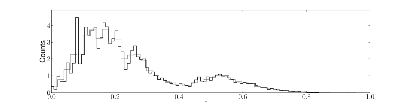
Figure 1: Spectroscopic redshift distribution of objects included in the training set (black line) and test set (gray line) normalized to the splitting rate.

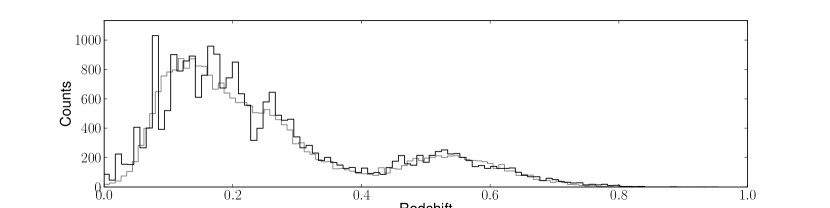
Figure 2: Redshift distribution of objects included in the blind test set, spectroscopic (black line) and photometric (gray line).

The results were evaluated using a standard set of statistical indicators applied to the quantity $\Delta z=\frac{z_{spec}-z_{phot}}{1+z_{spec}}$:

• the bias, defined as the mean value of the residuals $\Delta z$;

• the standard deviation ($\sigma$) of the residuals;

• the normalized median absolute deviation or $NMAD$ of the residuals, defined as $NMAD(\Delta z)=1.48\times Median\left(\left|\Delta z\right|\right)$.

As input photometric parameters (or features) we used the MAGAP_4 and MAGAP_6 aperture magnitudes ($u$, $g$, $r$, $i$), a choice which was based on our past experience, since almost always this combination lead to the best performances (Brescia et al., 2013, 2014b). However, it needs to be emphasized that an improvement in the performances of a machine learning method can be expected from an exhaustive exploration of the parameter space through feature selection (cf. Polsterer et al. 2014). This approach, however, is usually too much demanding in terms of computing time.

MLPQNA $z_{\text{phot}}$  are in excellent agreement with $z_{spec}$, as we show in Figs. 3 and 4, where the results of the experiment are summarized. The upper panel of Fig. 3 shows the predicted photometric redshift estimates versus the spectroscopic redshift values for all objects in the blind test set. In the lower panel of Fig. 3 the $z_{spec}$ is plotted vs. the residuals $\Delta z$. The underpopulated redshift bins, visible in Fig. 3, reflect the distribution of the spectroscopic sample which is less populated at redshift $\sim 0.22$ and $\sim 0.42$ (see Fig. 1 and Fig. 2).

In Fig. 4 we show the distribution of residuals which has a kurtosis of $1.8$ and a skewness of $7.07\times 10^{-16}$, i.e. a leptokurtic and symmetric distribution, as already found in the SDSS-DR9 case by applying the same method (Brescia et al., 2014b). In other words, the distribution reveals an over-density of objects in its central region (i.e. objects with a small error), which also reflects on the very low percentage of outliers and a low NMAD value (see below).

Overall, we find a bias of $9.9\times 10^{-4}$, a standard deviation of $0.0305$ and a NMAD of $0.021$. The $\sigma_{68}$ (i.e. the range in which falls the $68\%$ of the residuals) is $0.022$, smaller than the standard deviation, as it has to be expected from a leptokurtic distribution. Moreover, our method leads to a very small fraction of outliers, i.e. less than $0.39\%$ and $3.30\%$ using the $\left|\Delta z\right|>0.15$ and $\left|\Delta z\right|>2\sigma$ criteria, respectively. If we refer to the sample of objects with $IMAFLAGS\_ISO=0$, the bias, standard deviation and NMAD become $0.00072$, $0.0288$ and $0.0207$, respectively. While the fraction of outliers is of $0.32\%$ and $3.26\%$. Thus, although the present approach is quite immune to systematic effects in photometry, we find a small improvement in the statistics when the sources in the masked regions are removed from the analysis.

4 The photometric catalogue

To produce the final $z_{\text{phot}}$  catalogue, we initially considered the multi-source KiDS catalogue, i.e. sources detected in $r$-band and measured in all KiDS bands. However, it is important to underline that all empirical $z_{\text{phot}}$  prediction methods suffer from a poor capability to extrapolate outside the range of distributions imposed by the training sample. In literature, several approaches have been proposed to extend the applicability test of empirical methods outside the boundaries of the parameter space properly sampled by the spectroscopic KB (c.f. Vanzella et al. 2004; Hoyle et al. 2015). While useful in some cases, this artificial augmentation of the KB introduces a further level of complexity and leads to statistical biases which are difficult to evaluate and control.

In the available spectroscopic KB we found that $\sim 99\%$ of the KB objects falls within the following region of the parameter space:

• MAGAP_4_u $\leq 25.1$

• MAGAP_6_u $\leq 24.7$

• MAGAP_4_g $\leq 24.5$

• MAGAP_6_g $\leq 24.0$

• MAGAP_4_r $\leq 22.2$

• MAGAP_6_r $\leq 22.0$

• MAGAP_4_i $\leq 21.5$

• MAGAP_6_i $\leq 21.0$

Hence, to produce the final $z_{\text{phot}}$  catalogue, we have removed all the objects that do not match the above criteria in more than one band. The choice to retain objects with only one band not matching the above criteria was dictated by the need to maximize the number of objects with a redshift estimate and supported by the well tested robustness of the MLPQNA method against non detections or missing data (Cavuoti et al., 2012). In Table 1 we report the statistical indicators evaluated for two groups of objects: those having all data points falling within the above region (clean objects) and those (contaminated objects) with only one band falling outside of it. It appears evident that for a one-band failure there is only a small decrease of performance.

Subset	$|bias|$	$\sigma$	NMAD	Outliers $\%$	Outliers $\%$
				$|\Delta z|>0.15$	$|\Delta z|>2\sigma$
clean	0.0011	0.0303	0.0212	0.38	3.13
contaminated	0.0003	0.0339	0.0223	0.47	5.80

Table 1: Statistical indicators computed for two different subsets of the blind test set. The clean set includes only data for which the photometry falls within the limits listed in Sec. 4. The contaminated subset includes the objects which fall outside those limits in only one band.

However, in order to keep track of this effect, we include a $z_{\text{phot}}$  quality flag in the catalogue, set to $1$ for best quality (i.e. clean) and $0$ for worse quality (i.e. contaminated) objects.

The final $z_{\text{phot}}$  catalogue consists of $1,142,992$ objects ($699,155$ objects have all $IMAFLAGS\_ISO=0$ and $710,127$ with best quality).

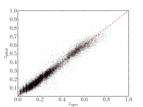
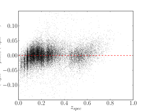
Figure 3: Upper panel: spectroscopic versus photometric redshifts for objects of the blind test set. Lower panel: spectroscopic redshift versus ($z_{\text{spec}}$-$z_{\text{phot}}$)/(1+$z_{\text{spec}}$) for the same objects.

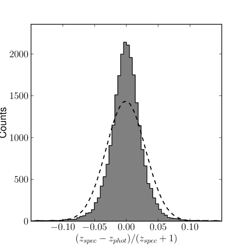
Figure 4: Histogram of ($z_{\text{spec}}$- $z_{\text{phot}}$)/(1+ $z_{\text{spec}}$) for objects of the blind test set. The dashed line represents the gaussian fit to the distribution.

5 Conclusions

In this work we applied the MLPQNA neural network to the ESO KiDS DR2 photometric galaxy data, using a knowledge base derived from the SDSS and GAMA spectroscopic samples, to produce a catalogue of photometric redshifts based on optical photometric data only. We obtained an overall $1\sigma$ uncertainty on $\Delta z=(z_{spec}-z_{phot})/(1+z_{spec})$ of $0.0305$ with a very small average bias of $9.9\times 10^{-4}$, a low $NMAD$ of $0.021$, and a low fraction of outliers ($0.39\%$ above the standard limit of $0.15$).

The trained network was then used to process all galaxies in the data set that populate a parameter space similar to that defined by the SDSS+GAMA spectroscopic sample, producing $z_{\text{phot}}$  estimates for about $1.1$ million KiDS galaxies. The catalogue will be made available on CDS VizieR facility.

Deriving photometric redshifts is an essential task when dealing with large samples of galaxies, such as that expected from the KiDS photometric survey. These redshifts are currently being used by the Kids collaboration for a variety of studies regarding the evolution of galaxy stellar masses, integrated colours, colour gradients and the structural parameters with redshift (Napolitano et al. in prep.). The characterization of how completeness and biases of the photo-z catalogue affect the final scientific goals is therefore postponed to later works. This types of studies will allow us to better constrain the processes leading to the (mass) growth of galaxies in the last half of the current age of the universe.

6 acknowledgements

The authors would like to thank the anonymous referee for extremely valuable comments and suggestions. Based on data products from observations made with ESO Telescopes at the La Silla Paranal Observatory under programme IDs 177.A-3016, 177.A-3017 and 177.A-3018, and on data products produced by Target/OmegaCEN, INAF-OACN, INAF-OAPD and the KiDS production team, on behalf of the KiDS consortium. OmegaCEN and the KiDS production team acknowledge support by NOVA and NWO-M grants. Members of INAF-OAPD and INAF-OACN also acknowledge the support from the Department of Physics & Astronomy of the University of Padova, and of the Department of Physics of Univ. Federico II (Naples). The authors would like to thank Amata Mercurio, Joachim Harnois-D raps and Peter Schneider for the very useful comments. CT has received funding from the European Union Seventh Framework Programme (FP7/2007-2013) under grant agreement n. 267251 Astronomy Fellowships in Italy (AstroFIt). This work was partially funded by the MIUR PRIN Cosmology with Euclid. MB acknowledges the support by the PRIN-INAF 2014 Glittering kaleidoscopes in the sky: the multifaceted nature and role of Galaxy Clusters.

References

- Ahn et al. (2012) Ahn, C. P., Alexandroff, R., Allende Prieto, C., et al. 2012, ApJS, 203, 21.
- Ahn et al. (2014) Ahn, C. P., Alexandroff, R., Allende Prieto, C., & et al., 2014, APJS, 211, 2, 17
- Bolton et al. (2012) Bolton, A. S., Schlegel, D. J., Aubourg, E., et al. 2012, AJ, 144, 144
- Bonfield et al. (2010) Bonfield, D.G., Sun, Y., Davey, N., Jarvis, M.J., Abdalla, F.B., Banerji, M., & Adams, R.G., 2010. MNRAS, 485, 987.
- Bertin & Arnouts (1996) Bertin, E., & Arnouts, S. 1996, A&A Supplement, 117, 393-404
- Brescia et al. (2012) Brescia, M., Cavuoti, S., Paolillo, M., Longo, G., Puzia, T., 2012. MNRAS, 421, 1155.
- Brescia et al. (2013) Brescia, M., Cavuoti, S., D’Abrusco, R., Longo, G., & Mercurio, A., 2013. ApJ, 772, 140.
- Brescia et al. (2014a) Brescia, M., Cavuoti, S., Longo, G., et al., 2014a. DAMEWARE: A web cyberinfrastructure for astrophysical data mining. PASP, Vol. 126, 942, pp. 783-797.
- Brescia et al. (2014b) Brescia, M., Cavuoti, S., Longo, G., De Stefano, V., 2014b, A catalogue of photometric redshifts for the SDSS-DR9 galaxies, A&A, Vol. 568, A126, 7 pages
- Capaccioli & Schipani (2011) Capccioli, M., & Schpani, P., 2011, The Messenger, 148, 2.
- Carliles et al. (2010) Carliles, S., Budavári, T., Heinis, S., Priebe, C., & Szalay, A. S. 2010. ApJ, 712, 511.
- Cavuoti et al. (2012) Cavuoti, S., Brescia, M., Longo, G., & Mercurio, A., 2012. A&A, 546, 13.
- Cavuoti et al. (2015) Cavuoti S., Brescia M., De Stefano V., Longo G., 2015. Experimental Astronomy, Springer, 39, 1, pp. 45-71
- Chen et al. (2012) Chen, Y.-M., Kauffmann, G., Tremonti, C. A., et al. 2012, MNRAS, 421, 314
- Connolly et al. (1995) Connolly, A.J., Csabai, I., Szalay, A.S., Koo, D.C., Kron, R.G., & Munn, J.A., 1995. AJ, 110, 2655.
- Csabai et al. (2003) Csabai, I., Budavári, T., Connolly, A.J., Szalay, A.S., et al., 2003. AJ, 125, 580.
- D’Abrusco et al. (2007) D’Abrusco, R., Longo, G., & Walton, N., 2007. ApJ, 663, 752.
- de Jong et al. (2013) de Jong et al. 2013. Experimental Astronomy, Springer, 35, 1-2, pp. 25-44.
- de Jong et al. (2015) de Jong et al. 2015, Submitted to A&A
- Driver et al. (2011) Driver, S. P., Hill, D. T., Kelvin, L. S., et al. 2011, MNRAS, 413, 971
- Freeman et al. (2009) Freeman, P.E., Newman, J.A., Lee, A.B., Richards, J.W., Schafer, C.M., 2009. MNRAS, 398, 4, 2012, 2021.
- Giannantonio et al. (2008) Giannantonio, T., Scranton, R., Crittenden, R.G., Nichol, R.C., Boughn, S.P., Myers, D., & Richards, G.T., 2008. Phys. Rev. D, 77, 123520.
- Hennawi et al. (2006) Hennawi, J.F., Strauss, M.A., Oguri, M., Inada, N., Richards, G.T., et al., 2006. AJ, 131, 1.
- Hildebrandt et al. (2010) Hildebrandt, H., Arnouts, S., Capak, P., Wolf, C. et al., 2010. A&A, 523, 31.
- Hopkins et al. (2013) Hopkins, A. M., Driver, S. P., Brough, S., et al., 2013, MNRAS, 430, 2047.
- Hoyle et al. (2015) Hoyle, E., et al., 2015. MNRAS, 450, 1, 305-316.
- Kaiser (2004) Kaiser, N., 2004. Pan-STARRS: a wide-field optical survey telescope array. Proceedings of SPIE, 5489, 11.
- Kuijken (2011) Kuijken, K., 2011. OmegaCAM: ESO’s newest imager. ESO Messenger, 146, 8.
- Geisser (1975) Geisser, S., 1975. Journal of the American Statistical Association, 70 (350), 320-328.
- La Barbera et al. (2008) La Barbera, F., de Carvalho, R. R., Kohl-Moreira, J. L., et al. 2008, PASP, 120, 681
- Laureijs et al. (2011) Laureijs, R., et al., 2011. Euclid Definition Study Report, ESA/SRE(2011)12, Issue 1.1, [arXiv:astro-ph/1110.3193].
- McFarland et al. (2013) McFarland, J. P., Verdoes-Kleijn, G., Sikkema, G., et al. 2013, Experimental Astronomy, 35, 45
- Myers et al. (2006) Myers, A.D., Brunner, R.J., Richards, G.T., Nichol, R.C., Schneider, D.P., Vanden Berk, D.E., Scranton, R., Gray, A.G., & Brinkmann, J., 2006. ApJ, 638, 622.
- Polsterer et al. (2014) Polsterer, K. L., Gieseke, F., Igel, C., Goto, T., 2014. ADASS XXIII, Vol. 485, p. 425.
- Scranton et al. (2005) Scranton, R., Menard, B., Richards, G.T., Nichol, R.C., Myers, A.D., et al., 2005. ApJ, 633, 2, 589.
- Vanzella et al. (2004) Vanzella, E., et al., 2004. A&A, 423, 761-776.
- Yéche et al. (2010) Yéche, C., Petitjean, P., Rich, J., Aubourg, E., Busca, N., et al., 2010. A&A, 523, 14.
- Wadadekar (2005) Wadadekar, Y., 2005. PASP, 117, 79.
- Way & Srivastava (2006) Way, M.J., & Srivastava, A.N., 2006. ApJ, 647, 102.