$Rev:128$ $Date:2015-05-2006:47:48-0400(Wed,20May2015)$

ACME: A Partially Periodic Estimator of
Avian & Chiropteran Mortality at Wind Turbines

1 Introduction

While wind energy has been employed for electricity production since the 1880s, it wasn’t until the oil crisis of the 1970s that commercial wind energy production was pursued actively in the United States. Wind energy use has grown rapidly since it began to be promoted as an alternative to fossil fuels and was accorded sponsorship by the state of California in the 1980s and by the Federal Government beginning in the late 1990s. Concerns about avian and chiropteran deaths caused by wind turbines emerged in the early 1990s [Howell and DiDonato, 1991], with widely varying estimates of the fatality rates, and studies were mounted to assess these rates as early as 1998 [Smallwood and Thelander, 2005]. Aggregate U.S. mortality estimates have been reported ranging from 20,000 to 573,000 birds annually [Erickson et al., 2001, 2005, Loss et al., 2013, Manville, 2009, Smallwood, 2013, Sovacool, 2012]. High profile lawsuits in such places as Altamont, CA (2007), Ventura, CA (2012), Nantucket Sound, MA (2012), Port Clinton, OH (2014) have brought the issue to national prominence.

The naïve approach to estimating turbine-related avian and chiropteran mortality— surveying periodically for bird and bat carcasses in designated areas near turbines at prescribed time intervals, and scaling the counts by time interval and study area— leads to grossly distorted estimates, for a variety of reasons. Some carcasses will be removed by scavengers before the survey, for example; some carcasses may be present but undetected at the time of the survey; some fatally injured birds or bats may survive long enough to alight outside the study area; and carcasses may be discovered whose death arose from other causes or during other time periods.

A number of investigators have developed modeling approaches leading to proposed adjustment formulas intended to overcome the distortions and biases of the naïve approach [Erickson et al., 1998, Johnson et al., 2003, Shoenfeld, 2004, Pollock, 2007, Huso, 2011], each embodying slightly different assumptions about the processes affecting carcass discovery. The wide variability of these estimation formulas leaves practitioners uncertain which of them (if any) to use. Here we explain the assumptions that underlie four commonly used estimation formulas, illustrate when each is appropriate and how they differ, and propose a new model-based Avian and Chiropteran Mortality Estimator called “ACME” that extends all four of them and introduces three new features to improve the reliability of mortality estimates: the diminishment of Field Technician (FT) discovery proficiency as carcasses age; the reduced rate of scavenger removal as carcasses age; and the possibility that some but not all carcasses present but undiscovered by FTs in one search may be discovered in a later search.

2 The Model Underlying the New Estimator

Suppose that carcasses arrive in a Poisson stream with intensity $m(t)$ that varies slowly with time $t$ and that they are removed (principally by scavengers) independently after random times $\tau_{j}$ with complimentary CDF ${\bar{F}}(t)={\mathsf{P}}[\tau_{j}>t]$. Suppose too that field technicians (FTs) mount blinded searches at a sequence of times $T_{i}$ at similar intervals $I_{i}=[T_{i}-T_{i{-}1}]$, and that the probability that a carcass of age $\tau$ will be discovered by an FT in such a search is $S(\tau)$ (which may depend on the carcass age $\tau$, but we are assuming for now that discovery is statistically independent of the scavenging removal process). Let $C_{i}$ denote the (random) number of carcasses actually discovered in the search at time $T_{i}$. Then the expected number of carcasses that arrive during the period and are discovered at time $T_{i}$ is

$$c^{0}_{i}:=\int_{T_{i{-}1}}^{T_{i}}m(t){\bar{F}}(T_{i}-t)S(T_{i}-t)\,dt.$$

Some existing mortality estimators (see Sections (2.1, 2.2)) embody the assumption that all carcasses that arrived prior to the previous search at time $T_{i{-}1}$ will have been removed by scavengers or discovered and removed by an FT in that earlier search, leaving none to “bleed through” from earlier periods to be removed or discovered in the current search at time $T_{i}$. Under that assumption, $c^{0}_{i}$ would be the expected count ${\mathsf{E}}[C_{i}]$. Other mortality estimators are based on a different assumption— that undiscovered and unremoved carcasses from earlier periods remain discoverable, so that $C_{i}$ may include both “new” carcasses from the current period and “old” ones that arrived during earlier periods. For $k\geq 1$ the expected number discovered at time $T_{i}$ that arrived during the $k$th previous period but were undiscovered in $k$ previous searches would be

$$c^{k}_{i}:=\int_{T_{i{-}k{-}1}}^{T_{i{-}k}}m(t){\bar{F}}(T_{i}-t)S(T_{i}-t)\prod_{0<n\leq k}\big{[}1-S(T_{i{-}n}-t)\big{]}\,dt$$

and the total expected carcass count for the $i$th search would be ${\mathsf{E}}[C_{i}]=c_{i}:=\sum_{k\geq 0}c^{k}_{i}$.

Evidence (see Section (5)) suggests that both the assumption that all carcasses bleed through for later discovery, and the assumption that none do, are wrong. We here introduce an intermediate possibility: that some fraction $0\leq{\mathfrak{B}}\leq 1$ do bleed through at each search, leading to expected carcass count

$${\mathsf{E}}[C_{i}]=c_{i}:=\sum_{k=0}^{\infty}{\mathfrak{B}}^{k}\int_{T_{i{-}k{-}1}}^{T_{i{-}k}}m(t){\bar{F}}(T_{i}-t)S(T_{i}-t)\prod_{0<n\leq k}\big{[}1-S(T_{i{-}n}-t)\big{]}\,dt.$$ (1)

For slowly-varying $m(t)\approx m$, this leads to a maximum likelihood estimate for the mean total mortality $m_{i}=\int_{T_{i{-}1}}^{T_{i}}m(t)dt\approx mI_{i}$ in period $(T_{i{-}1},T_{i}]$ of

$$\hat{M}^{\star}_{i} :=C_{i}/R^{\star}_{i},$$ (2a)

the carcass count $$C_{i} 1/R^{\star}_{i}$$ inflated by a factor given by the inverse of the “reduction factor”

$$R^{\star}_{i} :=\frac{1}{I_{i}}\sum_{k=0}^{\infty}{\mathfrak{B}}^{k}\int_{T_{i{-}k{-}1}}^{T_{i{-}k}}{\bar{F}}(T_{i}-t)S(T_{i}-t)\prod_{0<n\leq k}\big{[}1-S(T_{i{-}n}-t)\big{]}\,dt$$ (2b)

(so-called because on average the count $C_{i}\approx M_{i}R^{\star}_{i}$ will be the mortality $M_{i}$ reduced by the factor $R^{\star}_{i}$). For similar search intervals $I_{i}\approx I$, the $k$th term in this sum for $k\geq 1$ represents carcasses that arrived between $kI$ days and $(k+1)I$ days before the end of this search period, were unremoved by scavengers over that entire period, were undiscovered and yet remained discoverable in $k$ consecutive searches, and were finally discovered at time $T_{i}$. This will be a rare event unless $kI$ is quite small, so only a few terms of this sum are typically sufficient to achieve accuracy within a few percent. Simple approximations and truncation error bounds for them are given in Section (3.1).

Shoenfeld [2004] describes as periodic those estimators (including his own) based on the premise that all the undiscovered and unremoved carcasses remain discoverable, and the assumption that consecutive periods are similar. Our proposed estimator, intermediate between the periodic ones that assume 100% bleed-through and the aperiodic ones that assume 0%, might be described as partially-periodic.

2.1 Special Cases & Previous Estimators

Before turning to the general case, consider first the simple situation with constant removal rate (or hazard) $[-{\bar{F}}^{\prime}/{\bar{F}}](\tau)\equiv r$ and constant search proficiency $S(\tau)\equiv s$. Under this assumption that the scavenger removal rate and FT discover probabilities do not depend on carcass age $\tau$, the removal times must follow the exponential distribution $\tau\sim\mathsf{Ex}(r)$ with survival function ${\bar{F}}(t):={\mathsf{P}}[\tau>t]=\exp(-rt)$ for $t>0$ and mean removal time $\hat{t}:={\mathsf{E}}[\tau]=1/r$. In that case, for constant inter-search intervals $I_{i}\equiv I$, the reduction factor (2b) simplifies to a geometric series,

$$R^{\star}_{i} :=\frac{1}{I}\sum_{k=0}^{\infty}{\mathfrak{B}}^{k}\int_{(i-k-1)I}^{(i-k)I}\exp\big{(}-r(iI-t)\big{)}s(1-s)^{k}\,dt$$

$$=\frac{s~{}[e^{rI}-1]}{rI[e^{rI}-{\mathfrak{B}}(1-s)]}=\frac{s~{}\hat{t}~{}[e^{I/\hat{t}}-1]}{I[e^{I/\hat{t}}-{\mathfrak{B}}(1-s)]}.$$ (3)

In the case of zero bleed-through, ${\mathfrak{B}}=0$ and (3) leads to the estimator

$$\hat{M}_{i}^{P} =\frac{I\,C_{i}}{s~{}\hat{t}~{}[1-e^{-I/\hat{t}}]},$$ (4a)

that introduced by Pollock [2007] (under exponentially-distributed persistence).

Huso [2011] introduced a similar estimator $\hat{M}^{H}$ that differs in replacing the term $[1-e^{-I/\hat{t}}]$ by $\min\big{(}0.99,[1-e^{-I/\hat{t}}]\big{)}$. The two are identical whenever (as usual) search intervals $I$ are shorter than the mean removal times $\hat{t}$ times a factor of $\log 100\approx 4.6$, for then $[1-e^{-I/\hat{t}}]<0.99$ (otherwise Huso’s estimator $M_{i}^{H}$ is up to 1% higher than Pollock’s $M_{i}^{P}$).

In the case of full bleed-through, ${\mathfrak{B}}=1$ and (3) gives the “periodic” estimator introduced by Shoenfeld [2004],

$$\hat{M}_{i}^{S} =\frac{I\,C_{i}}{s~{}\hat{t}}\left[\frac{e^{I/\hat{t}}-1+s}{e^{I/\hat{t}}-1}\right].$$ (4b)

Finally, setting ${\mathfrak{B}}=1/(1-s)$ gives

$$\hat{M}_{i}^{E} =\frac{I\,C_{i}}{s~{}\hat{t}},$$ (4c)

the steady-state estimator introduced by Erickson et al. [1998].

2.2 Comparing Current Estimators

All four of the estimators $\hat{M}_{i}^{E}$, $\hat{M}_{i}^{S}$, $\hat{M}_{i}^{P}$, and $\hat{M}_{i}^{H}$ are special cases of (3), for specific values of ${\mathfrak{B}}$. Always

$$\big{[}1-e^{-(4.6\wedge I/\hat{t})}\big{]}\hat{M}_{i}^{H}=\hat{M}_{i}^{E}<\hat{M}_{i}^{S}<\hat{M}_{i}^{P}\leq\hat{M}_{i}^{H},$$ (5)

so all four estimators are within 5% if $I>3\hat{t}$ and within $58\%$ for $I>\hat{t}$. Under the assumptions of constant removal rate $-{\bar{F}}^{\prime}/{\bar{F}}\equiv r$ and constant searcher proficiency $S\equiv s$, the proposed new estimator $\hat{M}^{\star}$ of (2) also lies in the interval $[\hat{M}^{E}_{i},\hat{M}^{H}_{i}]$ for any $0\leq{\mathfrak{B}}\leq 1$.

Differences among the estimators will be substantial for shorter search intervals, however. For example, for search intervals substantially shorter than the mean scavenger removal time, $I\ll\hat{t}$ and so

$$\hat{M}^{H}_{i}\geq\hat{M}^{P}_{i}>(\hat{t}/I)\hat{M}^{E}_{i}\gg\hat{M}^{E}_{i},$$

and it will be important to assess bleed-through rate ${\mathfrak{B}}$ accurately. And, if the assumptions of constant removal rates and search proficiencies are incorrect, then the estimators may agree with each other but all be badly biased.

3 Variable Search Proficiency and Removal Rates

Both the assumptions of constant removal rate and of constant search proficiency, irrespective of carcass age, appear inconsistent with the observations presented in Section (5). In this section we show how to go beyond those assumptions.

3.1 Diminishing Proficiency

For many data sets the search proficiency $S(t)$ appears to diminish with increasing carcass age $t$. In Section (5) it is shown that the data are fit well by an exponentially decreasing success rate

$$S(t)=\exp\big{(}-a-bt\big{)}$$ (6)

for parameters $a,b\geq 0$ (logistic models gave very similar results). With this modeling choice, and for equal search intervals $I_{i}=I$ (say, with searches at times $T_{i}=iI$), the ACME estimator $\hat{M}^{\star}_{i}$ and reduction factor $R^{\star}_{i}$ of (2) take the form

$$\hat{M}^{\star}_{i} :=C_{i}/R^{\star}_{i},$$ (7a)

with

$$R^{\star}_{i} :=\sum_{k=0}^{\infty}{\mathfrak{B}}^{k}\int_{k}^{k+1}{\bar{F}}\big{(}xI\big{)}~{}e^{-a-xbI}\prod_{0<n\leq k}\Big{[}1-e^{-a-(x-n)bI}\Big{]}\,dx=\sum_{k=0}^{\infty}T^{\star}_{k},$$ (7b)

whose $k$th term $T^{\star}_{k}$ represents the fraction of carcasses that arrived in the search period ending at $T_{i{-}k}$ that are discovered at time $T_{i}$. Of particular importance (see Section (4)) is the first of these

$$T^{\star}_{0} =\int_{0}^{1}{\bar{F}}\big{(}xI\big{)}~{}e^{-a-xbI}\,dx,$$ (7c)

the fraction of carcasses discovered at the search ending the interval in which they arrived. Each $T^{\star}_{k}$ is expressible as the sum of $2^{k}$ terms of the form

$$Q^{\star}_{kmn} :={\mathfrak{B}}^{k}(-1)^{m+1}\int_{0}^{1}{\bar{F}}\big{(}(k+x)I\big{)}e^{-m\,(a+bI\,x)-n\,bI}\,dx$$ (8)

for suitable nonnegative integers $m,n$ that can be enumerated recursively: beginning with $(k,m,n)=(0,1,0)$, each entry $(k,m,n)$ generates at the next level $(k+1,m,n+1)$ and $(k+1,m+1,n+k+1)$. The first few terms are

$$T^{\star}_{0} =Q^{\star}_{010}$$ (9)

$$T^{\star}_{1} =Q^{\star}_{111}+Q^{\star}_{121}$$

$$T^{\star}_{2} =Q^{\star}_{212}+Q^{\star}_{223}+Q^{\star}_{222}+Q^{\star}_{233}$$

$$T^{\star}_{3} =Q^{\star}_{313}+Q^{\star}_{325}+Q^{\star}_{324}+Q^{\star}_{336}+Q^{\star}_{323}+Q^{\star}_{335}+Q^{\star}_{334}+Q^{\star}_{346}$$

The truncation error from using only the first $N$ terms $0\leq k<N$ of the infinite sum in (7b) is bounded by

$$0\leq\text{Truncation Error}\leq{\mathfrak{B}}^{N}{\bar{F}}(N\,I)\left[\frac{e^{-a-N\,bI}}{bI\vee(1-{\mathfrak{B}}e^{-bI})}\wedge(1-e^{-a})^{N}\right].$$ (10)

For the examples presented in Section (5), the truncation error bound is about 1% of $R^{\star}_{i}$ with $N=3$ terms, and about $0.1\%$ with $N=5$ terms.

3.2 Persistence Distributions

Bispo et al. [2013a, b] found (and we verify in Section (5.1) below) that log normal, log logistic, and Weibull distributions with decreasing hazard functions all fit empirical persistence data quite well, and that exponential distributions did not. Here we take the Weibull distribution, parametrized in the form

$${\bar{F}}(t):={\mathsf{P}}[\tau>t]=\exp\big{(}-(\rho t)^{\alpha}\big{)},\qquad t>0$$ (11)

for rate $\rho>0$ (in units of $\textsf{\,day}^{-1}$) and unitless shape parameter $\alpha>0$. For this distribution the key quantities $Q^{\star}_{kmn}$ from (8) needed to compute $R^{\star}_{i}$ are

$$Q^{\star}_{kmn} :={\mathfrak{B}}^{k}(-1)^{m+1}\int_{0}^{1}\exp\big{(}-(\rho(k+x)I)^{\alpha}-m\,(a+bI\,x)-n\,bI\big{)}\,dx,$$

easily evaluated numerically using Simpson’s quadrature rule or, for the particular values of $\alpha={\mathchoice{{\textstyle\frac{1}{2}}}{{\textstyle\frac{1}{2}}}{{\scriptscriptstyle\frac{1}{2}}}{{\scriptscriptstyle\frac{1}{2}}}}$ and $\alpha=1$, available explicitly in closed form:

$$Q^{\star}_{kmn} =\frac{2{\mathfrak{B}}^{k}(-1)^{m+1}}{\rho I}\exp\big{(}-ma+(mk-n)bI+\rho/4mb\big{)} \alpha={\mathchoice{{\textstyle\frac{1}{2}}}{{\textstyle\frac{1}{2}}}{{\scriptscriptstyle\frac{1}{2}}}{{\scriptscriptstyle\frac{1}{2}}}}$$ ()

$$\times\Bigg{\{}\frac{\rho}{2mb}\Big{[}e^{-mb(\sqrt{kI\rho}+\rho/2mb)^{2}}-e^{-mb(\sqrt{(k{+}1)I\rho}+\rho/2mb)^{2}}\Big{]}$$

$$\quad+2\sqrt{\frac{\pi\rho}{mb}}\Big{[}\Phi\Big{(}\sqrt{{2mb}/{\rho}}\big{(}\sqrt{\rho kI}+\frac{\rho}{2mb}\big{)}\Big{)}-\Phi\Big{(}\sqrt{{2mb}/{\rho}}\big{(}\sqrt{\rho(k{+}1)I}+\frac{\rho}{2mb}\big{)}\Big{)}\Big{]}\Bigg{\}}$$

$$Q^{\star}_{kmn} =\frac{(-1)^{m+1}e^{-m(a+bI)}}{(\rho+mb)I}\big{[}1-e^{-(\rho+mb)I}\big{]}\big{(}{\mathfrak{B}}e^{-rI}\big{)}^{k} \alpha=1$$ ()

where $\Phi(z)$ denotes the CDF for the standard $\mathsf{No}(0,1)$ normal distribution.

4 Mortality Estimates

Point estimates like $\hat{M}^{\star}$ of (2a) and (7a) are more informative when accompanied by some measure of their uncertainty. For example, Erickson et al. [1998] recommend reporting 50% and 90% interval estimates for mortality.

4.1 Interval Estimates for Mean Mortality $m_{i}$

In this section we will find interval estimates for the mean daily mortality rate $m_{i}$ based on observed carcass counts $C_{i}$. Such an estimate is given by a pair of functions $\mathtt{lo(c)}$ and $\mathtt{hi(c)}$ with the property that

$${\mathsf{P}}\big{[}m_{i}\in\mathtt{[lo(C_{i}),~{}hi(C_{i})]}~{}\big{]}\geq\gamma$$

for specified $\gamma$ (such as $0.5$ or $0.9$, per Erickson et al. [1998]). The common symmetric choice is to arrange that ${\mathsf{P}}\big{[}m_{i}<\mathtt{lo(C_{i})}\big{]}$ and ${\mathsf{P}}\big{[}m_{i}>\mathtt{hi(C_{i})}\big{]}$ are each below $(1{-}\gamma)/2$. Frequently in practice however mortality is low enough (or removal is rapid enough) that observed counts as low as zero or one are common [Huso et al., 2014], motivating interest in one-sided interval estimates with $\mathtt{lo(c)}\equiv 0$ and ${\mathsf{P}}\big{[}0\leq m_{i}\leq\mathtt{hi(C_{i})}\big{]}\geq\gamma$. A third option is to find the shortest interval that captures $m$ with probability at least $\gamma$.

Under the model introduced in Sections (2, 3) the mortality $M_{i}$ in the $i$th search period $(T_{i{-}1},T_{i}]$ has a Poisson distribution whose mean is the product $m_{i}I_{i}$ of the average daily mortality in that period $m_{i}$ and the search period length $I_{i}=(T_{i}-T_{i{-}1})$. If these rates and lengths are nearly constant (say, $m_{i}\approx m$ and $I_{i}\approx I$) over the period during which all the carcasses found at time $T_{i}$ arrived, and if the model parameters determining the reduction factor $R^{\star}_{i}$ of Eqn (7b) are nearly constant, then the conditional (given $m$) distribution of $C_{i}$ is

$$C_{i}\mid m\sim\mathsf{Po}\big{(}R^{\star}_{i}mI).$$

With conjugate Gamma prior distribution $m\sim\mathsf{Ga}(\xi,\lambda)$ (more on this below), the marginal distribution of carcass counts is negative binomial

$$C_{i}\sim\mathsf{NB}(\xi,\lambda/(\lambda+R^{\star}_{i}I))$$ (12)

and the posterior distribution for $m$ given $C_{i}$ is again Gamma but with new parameters:

$$m\mid C_{i} \sim\mathsf{Ga}(\xi+C_{i},\lambda+R^{\star}_{i}I).$$ (13)

The Objective Bayes reference prior distribution [Berger et al., 2009] for $m$, expressing no available prior or extrinsic information about it, is the improper $m\sim m^{-{\mathchoice{{\textstyle\frac{1}{2}}}{{\textstyle\frac{1}{2}}}{{\scriptscriptstyle\frac{1}{2}}}{{\scriptscriptstyle\frac{1}{2}}}}}$, the limiting case of the Gamma distribution with $\xi={\mathchoice{{\textstyle\frac{1}{2}}}{{\textstyle\frac{1}{2}}}{{\scriptscriptstyle\frac{1}{2}}}{{\scriptscriptstyle\frac{1}{2}}}}$ and $\lambda=0$. An alternative to Objective Bayes is to follow an Empirical Bayes approach [Robbins, 1955, Casella, 1985] using the evidence about $m$ reflected by previous observations of $\{C_{i}\}\mathrel{\mathop{\sim}\limits^{\mathrm{iid}}}\mathsf{NB}(\xi,\lambda/(\lambda+R^{\star}_{i}I))$ (typically this leads to shorter intervals, since they reflect more evidence about the average mortality rate $m$). It proceeds by making (often Maximum Likelihood) estimates $\hat{\xi}$ and $\hat{\lambda}$ of the parameters, and basing interval estimates for $m$ on these.

The resulting posterior $\gamma=50\%$ or $\gamma=90\%$ Credible Interval estimates for $m$ are of the form $\big{[}\mathtt{lo(C_{i}),~{}~{}hi(C_{i})}\big{]}$ with the functions $\mathtt{lo(c)}$ and $\mathtt{hi(c)}$ given by one of:

Objective Bayes, One-Sided:	$\mathtt{lo(c)=0}$
	$\mathtt{hi(c)=qgamma(\gamma,~{}c+{\mathchoice{{\textstyle\frac{1}{2}}}{{\textstyle\frac{1}{2}}}{{\scriptscriptstyle\frac{1}{2}}}{{\scriptscriptstyle\frac{1}{2}}}},~{}R^{\star}_{i}I)}$
Objective Bayes, Symmetric:	$\mathtt{lo(c)=qgamma((1-\gamma)/2,~{}c+{\mathchoice{{\textstyle\frac{1}{2}}}{{\textstyle\frac{1}{2}}}{{\scriptscriptstyle\frac{1}{2}}}{{\scriptscriptstyle\frac{1}{2}}}},~{}R^{\star}_{i}I)}$
	$\mathtt{hi(c)=qgamma((1+\gamma)/2,~{}c+{\mathchoice{{\textstyle\frac{1}{2}}}{{\textstyle\frac{1}{2}}}{{\scriptscriptstyle\frac{1}{2}}}{{\scriptscriptstyle\frac{1}{2}}}},~{}R^{\star}_{i}I)}$
Empirical Bayes, One-Sided:	$\mathtt{lo(c)=0}$
	$\mathtt{hi(c)=qgamma(\gamma,\hat{\xi}+c,\hat{\lambda}+R^{\star}_{i}I)}$
Empirical Bayes, Symmetric:	$\mathtt{lo(c)=qgamma((1-\gamma)/2,~{}\hat{\xi}+c,~{}\hat{\lambda}+R^{\star}_{i}I)}$
	$\mathtt{hi(c)=qgamma((1+\gamma)/2,~{}\hat{\xi}+c,~{}\hat{\lambda}+R^{\star}_{i}I)}$

where $\mathtt{qgamma(x,a,b)}$ [R Core Team, 2015] denotes the quantile function (inverse CDF) for the Gamma distribution. If the mortality rate $m(t)$ varies slowly enough that it may be considered constant over a longer period of time including some $n\geq 2$ search intervals of total length $I_{+}:=(T_{i}-T_{i{-}n})$, then the total number of carcasses $C_{+}:=\sum C_{i}$ found in the $n$ searches will again have a Poisson conditional distribution $C_{+}\mid m\sim\mathsf{Po}(R^{\star}_{i}I_{+}m)$ and a Negative Binomial marginal distribution $C_{+}\sim\mathsf{NB}(\xi,\lambda/(\lambda+R^{\star}_{i}I_{+}))$, and the posterior for $m$ will again be Gamma, $m\mid C_{+}\sim\mathsf{Ga}(\xi+C_{+},\lambda+R^{\star}_{i}I_{+})$. Quantiles of this Gamma distribution will determine Credible Intervals for $m$ that will be narrower by approximately a factor of $\sqrt{n}$ than those of (13), and so will specify $m$ to higher precision. The assumption of near-constancy of $m$ and the model parameters determining $R^{\star}_{i}$ would be violated for periods long enough to include changes in season, vegetation, or migratory patterns.

4.2 Interval Estimates for Mortality $M_{i}$

In this section we find interval estimates for the number $M_{i}$ of carcasses that arrived in the interval $(T_{i{-}1},T_{i}]$ based on the observed carcass count $C_{i}$. These will be wider than the intervals for $m_{i}$ of Section (4.1) because the aleatoric uncertainty and variability of mortality events typically exceeds the epistemic uncertainty about parameter values.

In general the $C_{i}$ carcasses discovered in the search at time $T_{i}$ may include both some of the $M_{i}$ carcasses that arrived during the period as well as some of those that arrived in earlier periods. Thus there is no way of making meaningful interval estimates about $M_{i}$ from $C_{i}$ alone, without making some assumptions about either the $\{M_{j}\}$ for $j<i$, i.e., about mortality in the recent past, or about the absence of bleed-through.

4.2.1 Classical Confidence Intervals (${\mathfrak{B}}=0$ only)

If, despite the evidence in Section (5), one assumes that no carcasses from earlier periods are ever discovered, i.e., if ${\mathfrak{B}}=0$, then $C_{i}\sim\mathsf{Bi}(M_{i},R^{\star}_{i})$ and classical Confidence Interval estimates are available for this binomial model without concern for mortality in earlier periods. For example, a 90% one-sided classical confidence interval for $M_{i}$ would be $[\mathtt{C_{i},hi(C_{i})}]$, where

$$\mathtt{hi(c)=}\inf\{M\geq c:~{}\mathtt{pbinom(c,~{}M,~{}R^{\star}_{i})}\leq 0.10\}$$

where $\mathtt{pbinom(x,n,p)}$ [R Core Team, 2015] denotes the CDF for the Binomial distribution.

4.2.2 Objective Bayes Credible Intervals (any ${\mathfrak{B}}$)

No simple classical confidence intervals for $M_{i}$ are available for the more realistic situation of ${\mathfrak{B}}>0$. Again, however, Objective Bayes and Empirical Bayes credible intervals may be constructed for $M_{i}$ based on the model of Sections (2, 3). Both Objective and Empirical Bayes posterior distribution for $M_{i}$, given $C_{i}$, are derived in Appendix A.2 and presented as

$${\mathsf{P}}[M_{i}=M\mid C_{i}=C]=c\times{}_{2}F_{1}(-C,-M;\xi-C-M;-z)$$ (14)

with $\xi={\mathchoice{{\textstyle\frac{1}{2}}}{{\textstyle\frac{1}{2}}}{{\scriptscriptstyle\frac{1}{2}}}{{\scriptscriptstyle\frac{1}{2}}}}$ for Objective Bayes or $\xi=\hat{\xi}$ for Empirical Bayes, for specified quantities $c$ and $z$ given in Eqns (21b, 21a), respectively, as explicit functions of $R^{\star}_{i}$ and $T^{\star}_{0}$ from Eqns (7b, 7c) (here ${}_{2}F_{1}(a,b;c;z)$ denotes Gauss’ hypergeometric function [NIST DLMF, , §15]). Setting $\mathtt{p(m|c)}:={\mathsf{P}}[M=m\mid C=c]$ from (14), credible intervals for $M$ are

$$[\mathtt{lo(C_{i})},\mathtt{hi(C_{i})}]$$ (15)

with

One-sided: $\mathtt{lo(c)=}0$ $\mathtt{hi(c)=}\min\{M:~{}\sum_{m\leq M}\mathtt{p(m|c)}\geq\gamma\}$ Symmetric: $\mathtt{lo(c)=}\max\{M:~{}\sum_{m\leq M}\mathtt{p(m|c)}\leq(1-\gamma)/2\}$ $\mathtt{hi(c)=}\min\{M:~{}\sum_{m\leq M}\mathtt{p(m|c)}\geq(1+\gamma)/2\}$

while Highest Posterior Density or HPD intervals [the shortest possible intervals with coverage probability $\gamma$, see Gelman et al., 2009, §2.3] for $M$ upon observing $C_{i}=c$ are available by sorting the values $\{\mathtt{p(m|c):}\,m\geq 0\}$ in decreasing order and identifying the smallest collection whose sum exceeds $\gamma$. Some of these distributions and intervals are shown in Figure (3). Similar Empirical Bayes results are available from Eqns (14, 21a) with estimated hyperparameters $\hat{\xi},\hat{\lambda}$.

In the absence of bleed-through (i.e., ${\mathfrak{B}}=0$) all found carcasses are “new” so necessarily $M_{i}\geq C_{i}$. It is shown in Section (A.2.2) that the number $(M_{i}-C_{i})$ of undiscovered carcasses then has the Negative Binomial distribution $(M_{i}-C_{i})\mid C_{i}\sim\mathsf{NB}\big{(}\xi+C,(\lambda+R^{\star}_{i}I)/(\lambda+I)\big{)}$, so

$${\mathsf{P}}[M_{i}=M\mid C_{i}=C]=\frac{\Gamma(\xi+M)}{\Gamma(\xi+C)~{}(M-C)!}(R^{\star}_{i}+\lambda/I)^{\xi+C}(1-R^{\star}_{i})^{M-C}(1+\lambda/I)^{-\xi-M}$$ (16)

from which credible intervals for $M_{i}$ are available. For example, the one-sided Objective Bayes interval is $[\mathtt{lo(C_{i})},\mathtt{hi(C_{i})}]$ with

$$\mathtt{lo(c)} =c\qquad\qquad\mathtt{hi(c)}=c+\mathtt{qnbinom(\gamma,c+1/2,R^{\star}_{i})}$$ (17a)

where $$\mathtt{qninom(p,alpha,prob)}$$ [R Core Team, 2015] denotes the quantile function for the negative binomial distribution. HPD regions are available with a search.

A more direct and less model-dependent Bayesian approach to finding the conditional distribution of $M$ given $C$ would be to begin with an improper uniform prior distribution for $M$ on the nonnegative integers $\{0,1,\dots\}$. The posterior distribution of the unobserved carcass count $(M-C)$, after observing $C\sim\mathsf{Bi}(M,R^{\star})$, then has the negative binomial distribution $(M_{i}-C_{i})\mid C_{i}\sim\mathsf{NB}(C_{i}+1,R^{\star}_{i})$, leading to very similar one-sided intervals with

$$\mathtt{lo(c)} =c\qquad\qquad\mathtt{hi(c)}=c+\mathtt{qnbinom(\gamma,c+1,R^{\star}_{i})}.$$ (17b)

5 Results from Altamont

Warren-Hicks et al. [2012] report on data taken from January 7 to April 30 of 2011 in the Altamont Pass Wind Resource Area in a study of the removal and discovery rates of aging bird and bat carcasses. One hundred and ten bird carcasses (predominantly brown-headed cowbirds, Molothrus Ater, with AOU code BHCO [Pyle and DeSante, 2014]) and 78 bat carcasses of disparate species were placed by Project Field Managers (PFMs), who then checked every few days to confirm whether or not each carcass remained in place. Field Technicians (FTs) would search for carcasses at approximately one week intervals, noting the species and location of those they discovered but not disturbing or removing them. Successive searches were conducted by different FTs who were unaware of any earlier carcass discoveries. This “integrated detection trial” or IDT design [Warren-Hicks et al., 2012, Chap. 2] afforded the possibility of exploring how removal rates and discovery probabilities may change over time.

5.1 Removal by scavengers

Figure (1) illustrates the removal of brown-headed cowbird carcasses by scavengers.

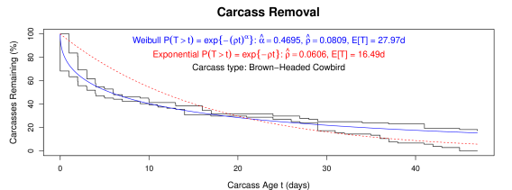
Figure 1: Empirical survival function showing removal of brown-headed cowbirds by scavengers (solid black stair-step lines), along with best Weibull distribution fit (solid blue line) and best Exponential distribution fit (dashed red line). Note Weibull fits well while Exponential does not.

Removals are interval censored: we only observe the times of the last recorded discovery of a carcass’s presence and the first of its absence. Thus the empirical survival function in Figure (1) consists of two black stair-step curves based on the earliest and latest possible times of removal consistent with the observations. The best Weibull distribution fit (see Section (A.1.1) for derivation of likelihood function (18) and MLEs),

$${\mathsf{P}}[\tau>t]=\exp\big{(}-(\rho t)^{\alpha}\big{)},\qquad\hat{\alpha}=0.4695,\quad\hat{\rho}=0.0809\textsf{\,day}^{-1}$$

is illustrated with the solid blue curve. Its mean of ${\mathsf{E}}[\tau]=27.97\textsf{\,day}$ is nearly twice that ($16.49\textsf{\,day}$) of the best exponential distribution fit, shown as a dashed red line. The exponential distribution model underestimates early removal rates and overestimates later ones. The estimated shape parameter $\hat{\alpha}=0.4695$ is $9.8$ standard errors away from the value $\alpha=1$ for the exponential distribution, making the exponential distribution and its assumption of constant removal rates entirely untenable. Best fits with log normal and log logistic were nearly indistinguishable from Weibull, so we present only Weibull results here.

5.2 Search Proficiency and Bleed-through

Figure (2) illustrates the search process by FTs.

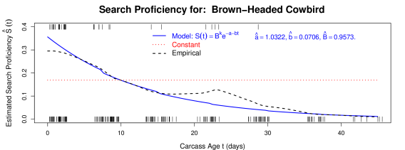
Figure 2: Empirical plot of search proficiency (dashed black line) for brown-headed cowbirds, along with best fit exponentially-decreasing curve (solid blue line) and best fit of a constant proficiency (dashed red line). Search successes (and failures) are shown as whiskers at the top (and bottom) of the plot, respectively. Note diminishing proficiency model fits data well while constant proficiency does not.

Short vertical dashes at the top and bottom of the plot indicate the times of successful and unsuccessful searches, respectively. Dashed black curve indicates a nonparametric estimator of time-dependent search proficiency, a moving-average double-exponential window estimator with width of 5 day. Proficiency exceeds $30\%$ initially, but falls off at about $7\%\textsf{\,day}^{-1}$.

Solid blue line shows best exponentially-decreasing fit, based on MLEs $\hat{\alpha}=0.4695$, $\hat{\rho}=0.0808$, and $\hat{\mathfrak{B}}=0.9573$ found by minimizing the negative log likelihood of Eqn (6) (see Section (A.1.2)). Dotted red line shows best constant-proficiency fit.

The deviance between the proposed model and the constant-proficiency model, a sub-model with $b=0$ and ${\mathfrak{B}}=1$, is $D=22.63$. By Wilks’ theorem [Wilks, 1938] this would have approximately a $\chi^{2}_{2}$ distribution with two degrees of freedom if the constant-rate model were correct, evidently an entirely untenable supposition with $P$-value about $10^{-5}$.

Carcasses were later discovered after an initial miss 9 times in this study, and after some earlier miss 12 times, confirming that some bleed-through occurred. Estimated bleed-through rate is $\hat{\mathfrak{B}}=95.73\%$. Evidence against full bleed-through ${\mathfrak{B}}=1$ is not strong enough to reject that possibility.

5.3 Mortality Estimation at Altamont

With the parameter estimates

$$\hat{\alpha}=0.4695\qquad\hat{\rho}=0.0809\textsf{\,day}^{-1}\qquad\hat{a}=1.0322\qquad\hat{b}=0.0706\textsf{\,day}^{-1}\qquad\hat{\mathfrak{B}}=0.9573$$

for the Weibull removal distribution ($\alpha,\rho$), exponentially falling search proficiency ($a,b$), and bleed-through rate (${\mathfrak{B}}$) (see Section (A.1)), we can use (7c) and a five-term approximation to (7b) to evaluate the Reduction Factor $R^{\star}_{i}$ for future searches at $7\textsf{\,day}$ intervals and the fraction of “new” carcasses $T^{\star}_{0}$ found in each search:

$$R^{\star}_{i} =0.2496\qquad\qquad T^{\star}_{0}=0.1740.$$

This suggests that about a quarter of the carcasses are discovered eventually, $17\%$ in the first search after arrival and the rest following bleed-through. This leads to the ACME adjusted mortality estimate

$$\hat{M}^{\star}_{i} =C_{i}/R^{\star}_{i}=4.01\times C_{i}$$

for a seven-day interval ending in a search at which $C_{i}$ brown-headed cowbird carcasses are discovered. From the same data and parameter estimates we can find reduction factors for other possible search interval lengths. For example, $R^{\star}_{i}=0.14$ and $\hat{M}^{\star}_{i}=6.9\times C_{i}$ for $I=14$-day searches, while $R^{\star}_{i}=0.47$ and $\hat{M}^{\star}_{i}=2.1\times C_{i}$ for $I=2$-day searches and $R^{\star}_{i}=0.57$, $\hat{M}^{\star}_{i}=1.8\times C_{i}$ for daily searches.

Figure (3) shows Objective Bayes posterior distributions (see Eqns (14, 21b)) for the Brown Cowbird mortality $M_{i}$ at Altamont in a 7-day search period in which $C_{i}$ carcasses were discovered for a few small values of $C_{i}$. Also given in the figure legends are point estimates $\hat{M}^{\star}_{i}=C_{i}/R^{\star}$, posterior means $\overline{M}^{\star}_{i}$, and 50% and 90% Objective Bayes posterior HPD interval estimates $I_{50}$ and $I_{90}$, derived in Section (A.2). These are also indicated in the figure by vertical arrows at $\hat{M}^{\star}_{i}$ and $\overline{M}^{\star}_{i}$ and by large red squares and filled blue disks illustrating $I_{50}$ and $I_{90}$, respectively.

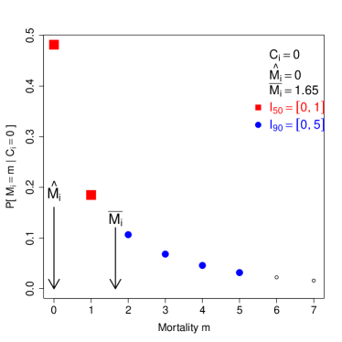
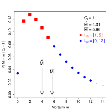
(a)	(b)
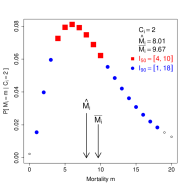
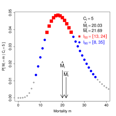
(c)	(d)

Figure 3: Objective Bayes posterior distribution of mortality $M_{i}$ for brown-headed cowbirds using $7$-day search intervals for carcass counts $C_{i}=0,1,2,5$ in panels (a), (b), (c), (d), respectively, based on Eqns (14, 21b). Large red squares show 50% HPD credible intervals, filled blue disks show 90% intervals. Downward arrows indicate ACME estimates $\hat{M}^{\star}_{i}=C_{i}/R^{\star}_{i}$ and Objective Bayes posterior means $\overline{M}^{\star}_{i}$.

6 Discussion

Commonly-used existing estimators give similar results if search intervals $I_{i}$ are much longer than the typical time $\hat{t}_{i}$ carcasses remain unremoved by scavengers, but differ drastically for more frequent searches because some of these estimators assume that undiscovered carcasses may remain from one search period to the next and some do not. Even when they agree they may be biased by disregarding the diminishing removal rate (by scavengers) and discovery proficiency (by Field Technicians) as carcasses age.

This work presents a new estimator called ACME (an acronym for Avian and Chiropteran Mortality Estimator) that includes many existing estimators as special cases, but that extends them in three ways: it reflects diminishing removal rates; it reflects decreasing discovery proficiency; and it allows for an arbitrary rate of “bleed-through” of carcasses that arrived before the current search period began. It also includes interval (as well as point) mortality estimates.

Mathematical formulas and computational methods are derived and presented here for both the initial problem of estimating the model’s five parameters on the basis of field discovery trials, and the continuing problem of constructing point and interval estimates for mortality on the basis of these parameter estimates and subsequent observed carcass counts.

Data Accessibility

A software package acme in the open-source R computer environment [R Core Team, 2015] is available at CRAN for finding maximum likelihood estimates of the model parameters and for evaluating the ACME estimator $\hat{M}^{\star}$, to make use of this estimator more accessible. Data used in preparation for this paper are included in that package. A guide to the design of integrated discovery trials suitable for supporting inference about the diminishing rates of discovery and removal (often unavailable from current discovery trial protocols) is also under development.

Appendix A Appendix: Computational Details

A.1 Parameter Estimates

In this section we construct maximum likelihood estimates from Integrated Detection Trial (IDT) data for the five parameters $(\alpha,\rho,~{}a,b,~{}{\mathfrak{B}})$ needed for the model of Sections (2, 3) to support point estimates $\hat{M}^{\star}_{i}:=C_{i}/R^{\star}_{i}$ of Eqn (7) and interval estimates $[\mathtt{lo(C_{i})},\mathtt{hi(C_{i})}]$ of Section (4.2) for mortality $M_{i}$.

A.1.1 Removal

Persistence times in this model have the Weibull distribution (11) with ${\mathsf{P}}[\tau>t]=\exp\big{(}-(\rho t)^{\alpha}\big{)}$ for $t>0$, depending on the two parameters $\alpha$ and $\rho$. Carcass placement times $t_{0}$ are known, but removal times $t_{r}$ (by scavengers) are generally not observed. The data available from an IDT bearing on $(\alpha,\rho)$ from the $k$th carcass consist of its placement time $t^{k}_{0}$, the last time $t^{k}_{p}\geq t^{k}_{0}$ of its known presence from discovery by either a FT or PFM, and the first time $t^{k}_{a}\geq t^{k}_{p}$ of its confirmed absence by a PFM (or $t^{k}_{a}=\infty$ if it remains present throughout the trial). The negative log likelihood function on the basis of these interval-censored data is

$$\ell_{\mathrm{rem}}(\alpha,\rho) =-\sum_{k}\log\left\{e^{-[\rho(t^{k}_{p}-t^{k}_{0})]^{\alpha}}-e^{-[\rho(t^{k}_{a}-t^{k}_{0})]^{\alpha}}\right\}$$

$$=\rho^{\alpha}\sum_{k}(t^{k}_{p}-t^{k}_{0})^{\alpha}-\sum_{k}\log\left\{1-e^{\rho^{\alpha}[(t^{k}_{p}-t^{k}_{0})^{\alpha}-(t^{k}_{a}-t^{k}_{0})^{\alpha}]}\right\}.$$ (18)

The MLEs presented in Section (5.1) are the minimizing values $(\hat{\alpha},\hat{\rho})$, easily found by a numeric search, along with approximate standard errors from the inverse Hessian.

A.1.2 Discovery

The probability of discovery of a $t$-day-old carcass present at an FT’s search is given in (6) as $S(t)=\exp\big{(}-a-bt\big{)}$, depending on the two parameters $(a,b)$.

Again denote by $t_{0}$ the placement time for a particular carcass (say, the $k$th) and by $t_{p}$ the last time it is known to be present. Let $m_{0}:=\min\{n:T_{n}\geq t_{0}\}$ and $m^{*}:=\max\{n\geq m_{0}:T_{n}\leq t_{p}$ index the first and last FT searches at which the carcass is present, and let $m_{*}:=\max\{n\geq m_{0}:~{}D_{n}=1\}$ index the last successful search (or $m_{*}=m_{0}$ if it is never discovered). Introduce the short-hand notation $p_{n}(a,b):=\exp\big{(}-a-b(T_{n}-t_{0})\big{)}$ for the probability of discovery at the $n$th search, for $m_{0}\leq n\leq m^{*}$. For a carcass that arrived in an earlier search period to be discovered now it must have been undiscovered and also “bled through” at each previous search. Set $D_{n}=1$ for a successful discovery and $D_{n}=0$ for a failure. Then the probability of the observed sequence of successes and failures for the $k$th carcass, as a function of $(a,b,{\mathfrak{B}})$, is the sum over all possible indices $m$ of the last search time $T_{m}$ at which the carcass bleeds through,

$$\begin{split}{\mathcal{L}}^{k}_{\mathrm{disc}}(a,b,{\mathfrak{B}})=(1-{\mathfrak{B}})\sum_{m_{*}\leq m<m^{*}}&{\mathfrak{B}}^{m-m_{0}}\prod_{m_{0}\leq n\leq m}p_{n}(a,b)^{D_{n}}(1-p_{n}(a,b))^{1-D_{n}}\\ +&{\mathfrak{B}}^{m^{*}-m_{0}}\prod_{m_{0}\leq n\leq m^{*}}p_{n}(a,b)^{D_{n}}(1-p_{n}(a,b))^{1-D_{n}}.\end{split}$$ (19a)

The negative log likelihood contribution for all carcass combined is the sum

$$\ell_{\mathrm{disc}}(a,b,{\mathfrak{B}}) =\sum_{k}-\log{\mathcal{L}}^{k}_{\mathrm{disc}}(a,b,{\mathfrak{B}}).$$ (19b)

The MLEs presented in Section (5.2) are the minimizing values $(\hat{a},\hat{b},\hat{\mathfrak{B}})$.

A.2 Posterior Distribution of Mortality

In this section we consider the posterior distribution of the mortality $M_{i}$ in a fixed period $(T_{i{-}1},T_{i}]$ of length $I_{i}=(T_{i}-T_{i{-}1})$ days, conditional upon the observed count $C_{i}$ in the search at time $T_{i}$, in order to find interval estimates for $M_{i}$. To make the notation less cumbersome we omit the subscripts “$i$”.

The total number $C$ of carcasses discovered in the search will in general be a sum $C=C_{\text{\tiny new}}+C_{\text{\tiny old}}$ of “new” carcasses that arrived during the current interval and “old” ones that arrived in earlier periods, but were undiscovered and unremoved in earlier periods. In this model the mortality $M\sim\mathsf{Po}(mI)$ in a particular search interval has a Poisson distribution with uncertain mean $mI$ for a daily average rate $m\geq 0$ which varies sufficiently slowly from one interval to another that we may treat it as constant over the arrival times of all the carcasses discovered in a particular search. We employ a Gamma prior distribution $m\sim\mathsf{Ga}(\xi,\lambda)$ for $m$, usually with the Objective Bayes prior parameters $\xi=1/2$, $\lambda=0$ [Berger et al., 2009].

Each of the $M$ carcasses that arrive during the period has probability $T^{\star}_{0}$ of being discovered in the current search, probability $(R^{\star}-T^{\star}_{0})$ of being discovered in some future search, and probability $(1-R^{\star})$ of never being discovered. Thus the model may be described:

$$m \sim\mathsf{Ga}(\xi,~{}\lambda)$$ Average daily mortality

$$C_{\text{\tiny old}} \sim\mathsf{Po}\big{(}m(R^{\star}-T^{\star}_{0})I\big{)}$$ From all previous periods

$$M \sim\mathsf{Po}(mI)$$ Mortality this period

$$C_{\text{\tiny new}}\mid M \sim\mathsf{Bi}(M,T^{\star}_{0}) M$$ New count, conditional on

$$C_{\text{\tiny new}} \sim\mathsf{Po}(mT^{\star}_{0}I)$$ New count, marginal

$$C =C_{\text{\tiny new}}+C_{\text{\tiny old}}$$ (new + old), indep.

where $R^{\star}\geq T^{\star}_{0}$ are given in Eqns (7b, 7c).

A.2.1 Possible bleed-through (${\mathfrak{B}}>0$)

First consider the case where $R^{\star}>T^{\star}_{0}$, and in particular ${\mathfrak{B}}>0$, so the mortality $M$ may take any nonnegative integer value— even $M<C$, since some or even all of the $C$ discovered carcasses may have arrived in earlier search intervals. Summing over the possible number $x=C_{\text{\tiny new}}$ of new carcasses and integrating over the uncertain mean daily mortality $m$,

$${\mathsf{P}}[C =C,M=M]$$

$$=\sum_{x=0}^{C\wedge M}\int_{0}^{\infty}\left\{\frac{m^{\xi-1}\lambda^{\xi}}{\Gamma(\xi)}e^{-m\lambda}\right\}\left\{\frac{(mI)^{M}}{M!}e^{-mI}\right\}\left\{\binom{M}{x}(T^{\star}_{0})^{x}(1-T^{\star}_{0})^{M-x}\right\}$$

$$\qquad\times\left\{\frac{[(R^{\star}-T^{\star}_{0})mI]^{C-x}}{(C-x)!}e^{-{(R^{\star}-T^{\star}_{0})mI}}\right\}\,dm$$

$$=\sum_{x=0}^{C\wedge M}\frac{\Gamma(\xi+C+M-x)}{\Gamma(\xi)(C-x)!(M-x)!x!}\quad\frac{\lambda^{\xi}(T^{\star}_{0})^{x}(R^{\star}-T^{\star}_{0})^{C-x}(1-T^{\star}_{0})^{M-x}I^{C+M-x}}{[\lambda+(R^{\star}-T^{\star}_{0}+1)I]^{\xi+C+M-x}}$$

$$=c\times\sum_{x=0}^{C\wedge M}\frac{\Gamma(\xi+C+M-x)}{(C-x)!(M-x)!x!}~{}z^{x}$$

$$=c\times\frac{\Gamma(\xi+C+M)}{C!\,M!}~{}{}_{2}F_{1}(-C,-M;1-\xi-C-M;-z)$$ (20a)

where $${}_{2}F_{1}(a,b;c;z)$$ is Gauss’ hypergeometric function [NIST DLMF, , §15] and where

$$c=\frac{\lambda^{\xi}(R^{\star}-T^{\star}_{0})^{C}(1{-}T^{\star}_{0})^{M}I^{C+M}}{\Gamma(\xi)[\lambda+(R^{\star}-T^{\star}_{0}+1)I]^{\xi+C+M}}\qquad z=\frac{T^{\star}_{0}[\lambda+(R^{\star}-T^{\star}_{0}+1)I]}{(1{-}T^{\star}_{0})(R^{\star}-T^{\star}_{0})\,I}.$$

The induced marginal distribution of $C\sim\mathsf{Po}\big{(}mR^{\star}I)$ is negative binomial,

$${\mathsf{P}}[C=C]=\frac{\Gamma(\xi+C)}{\Gamma(\xi)~{}C!}\lambda^{\xi}(R^{\star}I)^{C}(\lambda+R^{\star}I)^{-\xi-C}.$$ (20b)

Dividing (20a) by (20b) gives the conditional distribution for mortality $M$ given a carcass count of $C$:

$${\mathsf{P}}[M =M\mid C=C]=c\times{}_{2}F_{1}(-C,-M;1-\xi-C-M;-z)$$ (14)

with $c$ and $z$ given by

$$\begin{split}c&=\frac{\Gamma(\xi+C+M)(\lambda+R^{\star}I)^{\xi+C}(R^{\star}-T^{\star}_{0})^{C}(1-T^{\star}_{0})^{M}\,I^{M}}{\Gamma(\xi+C)~{}M!~{}(R^{\star})^{C}[\lambda+(R^{\star}-T^{\star}_{0}+1)I]^{\xi+C+M}}\\ z&=\frac{T^{\star}_{0}~{}[\lambda+(R^{\star}-T^{\star}_{0}+1)I]}{(1{-}T^{\star}_{0})(R^{\star}-T^{\star}_{0})~{}I}.\end{split}$$ (21a)

For the Objective Bayes reference values $$\xi={\mathchoice{{\textstyle\frac{1}{2}}}{{\textstyle\frac{1}{2}}}{{\scriptscriptstyle\frac{1}{2}}}{{\scriptscriptstyle\frac{1}{2}}}} \lambda=0 c z I$$ and the distribution is again given by (14), but and are a bit simpler and don’t depend on the search interval length :

$$\begin{split}c&=\frac{\Gamma({\mathchoice{{\textstyle\frac{1}{2}}}{{\textstyle\frac{1}{2}}}{{\scriptscriptstyle\frac{1}{2}}}{{\scriptscriptstyle\frac{1}{2}}}}+C+M)(R^{\star})^{{\mathchoice{{\textstyle\frac{1}{2}}}{{\textstyle\frac{1}{2}}}{{\scriptscriptstyle\frac{1}{2}}}{{\scriptscriptstyle\frac{1}{2}}}}}(R^{\star}-T^{\star}_{0})^{C}(1-T^{\star}_{0})^{M}}{\Gamma({\mathchoice{{\textstyle\frac{1}{2}}}{{\textstyle\frac{1}{2}}}{{\scriptscriptstyle\frac{1}{2}}}{{\scriptscriptstyle\frac{1}{2}}}}+C)~{}M!~{}(R^{\star}-T^{\star}_{0}+1)^{{\mathchoice{{\textstyle\frac{1}{2}}}{{\textstyle\frac{1}{2}}}{{\scriptscriptstyle\frac{1}{2}}}{{\scriptscriptstyle\frac{1}{2}}}}+C+M}}\\ z&=\frac{T^{\star}_{0}(R^{\star}-T^{\star}_{0}+1)}{(1{-}T^{\star}_{0})(R^{\star}-T^{\star}_{0})}.\end{split}$$ (21b)

This is well-defined even though, by (12), the marginal predictive distribution of $C$ is degenerate for $\lambda=0$. Objective Bayes $100\gamma\%$ credible intervals for $M$ are presented in Section (4.2.2) and illustrated in Figure (3), based on the conditional distribution of $M$ (for specified $C$) given in Eqns (14, 21b).

A.2.2 No bleed-through (${\mathfrak{B}}=0$)

For the remaining case of $R^{\star}=T^{\star}_{0}$ where only “new” carcasses can be found, the sum of Eqn (20a) reduces to the single term $x=C\leq M$, so only values $M\geq C$ are possible and for these Eqn (14) becomes:

$${\mathsf{P}}[M=M\mid C=C]=\frac{\Gamma(\xi+M)}{\Gamma(\xi+C)~{}(M-C)!}(R^{\star}+\lambda/I)^{\xi+C}(1-R^{\star})^{M-C}(1+\lambda/I)^{-\xi-M}.$$ (16)

The number $M-C$ of undiscovered carcasses will have a negative binomial conditional distribution $(M-C)\mid C\sim\mathsf{NB}\big{(}\xi+C,(\lambda+R^{\star}I)/(\lambda+I)\big{)}$ or, for the Objective Bayes case of $\xi={\mathchoice{{\textstyle\frac{1}{2}}}{{\textstyle\frac{1}{2}}}{{\scriptscriptstyle\frac{1}{2}}}{{\scriptscriptstyle\frac{1}{2}}}}$, $\lambda=0$, $(M-C)\mid C\sim\mathsf{NB}\big{(}C+{\mathchoice{{\textstyle\frac{1}{2}}}{{\textstyle\frac{1}{2}}}{{\scriptscriptstyle\frac{1}{2}}}{{\scriptscriptstyle\frac{1}{2}}}},R^{\star}\big{)}$, justifying the interval estimate for $M$ given in Eqn (17a).

Last edited: , 19:25 EDT

References

- Berger et al. [2009] J. O. Berger, J. M. Bernardo, and D. Sun. The formal definition of reference priors. Ann. Stat., 37(2):905–938, 2009.
- Bispo et al. [2013a] R. Bispo, J. Bernardino, T. A. Marques, and D. Pestana. Discrimination between parametric survival models for removal times of bird carcasses in scavenger removal trials at wind turbines sites. In J. Lita da Silva, F. Caeiro, I. Natáio, C. A. Braumann, M. L. Esquível, and J. Mexia, editors, Advances in Regression, Survival Analysis, Extreme Values, Markov Processes and Other Statistical Applications, Studies in Theoretical and Applied Statistics, chapter 4, Part II. Springer-Verlag, 2013a. ISBN 978-3-642-34903-4.
- Bispo et al. [2013b] R. Bispo, J. Bernardino, T. A. Marques, and D. Pestana. Modeling carcass removal time for avian mortality assessment in wind farms using survival analysis. Environmental and Ecological Statistics, 20(1):147–165, 2013b. doi: 10.1007/s10651-012-0212-5.
- Casella [1985] G. Casella. An introduction to empirical bayes data analysis. American Statistician, 39(2):83–87, 1985. doi: 10.2307/2682801.
- Erickson et al. [1998] W. P. Erickson, M. D. Strickland, G. D. Johnson, and J. W. Kern. Examples of statistical methods to assess risks of impacts to birds from wind plants. In PNAWPPM-III: Proceedings of the Avian-Wind Power Planning Meeting III, San Diego, CA. National Wind Coordinating Committee Meeting, May 1998, Washington, DC, 1998. Prepared for the Avian Subcommittee of the National Wind Coordinating Committee by LGL, Ltd., King City, Ont.
- Erickson et al. [2001] W. P. Erickson, G. D. Johnson, M. D. Strickland, D. P. Young, Jr., K. J. Sernka, and R. E. Good. Avian collisions with wind turbines: a summary of existing studies and comparisons to other sources of avian collision mortality in the United States, 2001. On-line at http://www.west-inc.com/reports/avian\_collisions.pdf.
- Erickson et al. [2005] W. P. Erickson, G. D. Johnson, and D. P. Young, Jr. A summary and comparison of bird mortality from anthropogenic causes with an emphasis on collisions. Technical Report PSW-GTR-191, U.S. Department of Agriculture, Washington, D.C., 2005.
- Erickson et al. [2008] W. P. Erickson, J. D. Jeffrey, and V. K. Poulton. Puget sound energy wild horse wind facility post-construction avian and bat monitoring: First annual report january–december 2007. Technical report, Puget Sound Energy (Ellensburg, WA 98296) and Wild Horse Wind Facility Technical Advisory Committee (Kittitas County, WA); prepared by Western EcoSystems Technology Inc, Cheyenne, WY, Jan 2008.
- Etterson [2013] M. A. Etterson. Hidden Markov models for estimating animal mortality from anthropogenic hazards. Ecological Applications, 23(8):1915–1925, 2013. doi: 10.1890/12-1166.1.
- Gelman et al. [2009] A. Gelman, J. B. Carlin, H. S. Stern, and D. B. Rubin. Bayesian Data Analysis. Taylor & Francis, Boca Raton, FL, 2nd edition, 2009. ISBN 1-58488-388-X.
- Howell and DiDonato [1991] J. A. Howell and J. E. DiDonato. Assessment of avian use and mortality related to wind turbine operations, Altamont Pass, Alameda and Contra Costa Counties, California, September 1988 through August 1989, 1991. Final Report to U.S. WindPower, Inc., Livermore, Calif.
- Huso [2011] M. M. P. Huso. An estimator of wildlife fatality from observed carcasses. Environmetrics, 22(3):318–329, 2011. doi: 10.1002/env.1052.
- Huso et al. [2014] M. M. P. Huso, D. H. Dalthorp, D. A. Dail, and L. J. Madsen. Estimating wind-turbine caused bird and bat fatality when zero carcasses are observed. Ecological Applications, pages On–line only, 2014. doi: 10.1890/14-0764.1.
- Johnson et al. [2003] G. D. Johnson, W. P. Erickson, M. D. Strickland, M. F. Shepherd, D. A. Shepherd, and S. A. Sarappo. Mortality of bats at a large-scale wind power development at Buffalo Ridge, Minnesota. The American Midland Naturalist, 150(2):332–342, 2003. doi: 10.1674/0003-0031(2003)150[0332:MOBAAL]2.0.CO;2.
- Korner-Nievergelt et al. [2015] F. Korner-Nievergelt, O. Behr, R. Brinkmann, M. A. Etterson, M. M. P. Huso, D. H. Dalthorp, P. Korner-Nievergelt, T. Roth, and I. Niermann. Mortality estimation from carcass searches using the R-package carcass — a tutorial. Wildlife Biology, 21(1):30–43, 2015. doi: 10.2981/wlb.00094.
- Loss et al. [2013] S. R. Loss, T. Will, and P. P. Marra. Estimates of bird collision mortality at wind facilities in the contiguous United States. Biological Conservation, 168:201–209, 2013. doi: 10.1016/j.biocon.2013.10.007.
- Manville [2009] A. Manville, II. Towers, turbines, power lines, and buildings— steps being taken by the U.S. Fish and Wildlife Service to avoid or minimize take of migratory birds at these structures. In Proceedings of the Fourth International Partners in Flight Conference: Tundra to Tropics, pages 262–272, 2009.
- Olver et al. [2010] F. W. J. Olver, D. W. Lozier, R. F. Boisvert, and C. W. Clark, editors. NIST Handbook of Mathematical Functions. Cambridge Univ. Press, New York, NY, 1.0.9 edition, 2010. ISBN 978-0-521-19225-5. URL http://dlmf.nist.gov/. Print companion to [NIST DLMF, ].
- Péron et al. [2013] G. Péron, J. E. Hines, J. D. Nichols, W. L. Kendall, K. A. Peters, and D. S. Mizrahi. Estimation of bird and bat mortality at wind-power farms with superpopulation models. Journal of Applied Ecology, 50:902–911, 2013. doi: 10.1111/1365-2664.12100.
- Pollock [2007] K. H. Pollock. Recommended formulas for adjusting fatality rates. In California Guidelines for Reducing Impacts to Birds and Bats from Wind Energy Development, pages 117–118, Appendix F. California Energy Commission, Renewables Committee, and Energy Facilities Siting Division, and California Department of Fish and Game, Resources Management and Policy Division, 2007. CEC Final Report, Document CEC-700-2007-008-CMF.
- Pyle and DeSante [2014] P. Pyle and D. F. DeSante. List of North American birds and alpha codes according to American Ornithologists’ Union taxonomy through the 54th AOU Supplement [Updated 2014-09-29]. American Ornithologists’ Union, Point Reyes Station, CA, 2014. Available from http://www.birdpop.org/alphacodes.htm.
- R Core Team [2015] R Core Team. R: A Language and Environment for Statistical Computing. R Foundation for Statistical Computing, Vienna, AT, 2015. URL http://www.R-project.org.
- [23] NIST DLMF. NIST Digital Library of Mathematical Functions. Release 1.0.9, 2014. URL http://dlmf.nist.gov/. Online companion to [Olver et al., 2010], at URL http://dlmf.nist.gov/.
- Robbins [1955] H. Robbins. An empirical Bayes approach to statistics. In J. Neyman, editor, Proc. Third Berkeley Symp. Math. Statist. Prob., volume 1, pages 157–164. University of California Press, Berkeley, CA, 1955. URL http://projecteuclid.org/euclid.bsmsp/1200501653.
- Shoenfeld [2004] P. S. Shoenfeld. Suggestions regarding avian mortality extrapolation. On-line at http://www.wvhighlands.org/Birds/SuggestionsRegardingAvianMortalityExtrapolation.pdf, 2004.
- Smallwood [2013] K. S. Smallwood. Comparing bird and bat fatality-rate estimates among North American wind-energy projects. Wildlife Society Bulletin, 37(1):19–33, 2013. doi: 10.1002/wsb.260.
- Smallwood and Thelander [2005] K. S. Smallwood and C. G. Thelander. Bird Mortality at the Altamont Pass Wind Resource Area: March 1998 – September 2001. National Renewable Energy Laboratory (NREL), Golden, Colorado 80401, 2005. URL http://www.osti.gov/bridge. Subcontract Report NREL/SR-500-36973.
- Sovacool [2012] B. K. Sovacool. The avian benefits of wind energy: a 2009 update. Renewable Energy, 49:19–24, 2012. doi: 10.1016/j.renene.2012.01.074.
- Warren-Hicks et al. [2012] W. Warren-Hicks, J. Newman, R. L. Wolpert, B. Karas, and L. Tran. Improving Methods for Estimating Fatality of Birds and Bats at Wind Energy Facilities, 2012. URL http://www.energy.ca.gov/2012publications/CEC-500-2012-086/CEC-500-2012-086.pdf. California Wind Energy Association publication CEC-500-2012-086.
- Wilks [1938] S. S. Wilks. The large-sample distribution of the likelihood ratio for testing composite hypotheses. Ann. Math. Statist., 9(1):60–62, 1938.
Last edited: , \two@digits19:\two@digits25 EDT