11email: jdejong@strw.leidenuniv.nl 22institutetext: Kapteyn Astronomical Institute, University of Groningen, P.O. Box 800, 9700 AV Groningen, the Netherlands 33institutetext: INAF - Osservatorio Astronomico di Capodimonte, Via Moiariello 16 -80131 Napoli, Italy 44institutetext: INAF - Osservatorio Astronomico di Padova, via dell’Osservatorio 5, 35122 Padova, Italy 55institutetext: Scottish Universities Physics Alliance, Institute for Astronomy, University of Edinburgh, Royal Observatory, Blackford Hill, Edinburgh EH9 3HJ, United Kingdom 66institutetext: Argelander-Institut für Astronomie, Auf dem Hügel 71, D-53121 Bonn, Germany 77institutetext: Department of Physics, University Federico II, Via Cinthia 6, 80126 Napoli, Italy 88institutetext: Agenzia Spaziale Italiana - Science Data Center, Via del Politecnico snc, 00133 Roma, Italy 99institutetext: Department of Physics & Astronomy, University College London, Gower Street, London WC1E 6BT, United Kingdom 1010institutetext: Department of Physics and Astronomy, University of British Columbia, BC V6T 1Z1, Canada 1111institutetext: Mullard Space Science Laboratory, University College London, Holmbury St Mary, Dorking, Surrey RH5 6NT, United Kingdom 1212institutetext: School of Physics and Astronomy, Queen Mary University of London, Mile End Road, London E1 4NS, United Kingdom
The first and second data releases of the Kilo-Degree Survey
Abstract
Context. The Kilo-Degree Survey (KiDS) is an optical wide-field imaging survey carried out with the VLT Survey Telescope and the OmegaCAM camera. KiDS will image 1500 square degrees in four filters (), and together with its near-infrared counterpart VIKING will produce deep photometry in nine bands. Designed for weak lensing shape and photometric redshift measurements, its core science driver is mapping the large-scale matter distribution in the Universe back to a redshift of 0.5. Secondary science cases include galaxy evolution, Milky Way structure, and the detection of high-redshift clusters and quasars.
Aims. KiDS is an ESO Public Survey and dedicated to serving the astronomical community with high-quality data products derived from the survey data. Public data releases, the first two of which are presented here, are crucial for enabling independent confirmation of the survey’s scientific value. The achieved data quality and initial scientific utilization are reviewed in order to validate the survey data.
Methods. A dedicated pipeline and data management system based on Astro-WISE, combined with newly developed masking and source classification tools, is used for the production of the data products described here. Science projects based on these data products and preliminary results are outlined.
Results. For 148 survey tiles (160 sq.deg.) stacked images have been released, accompanied by weight maps, masks, source lists, and a multi-band source catalogue. Limiting magnitudes are typically 24.3, 25.1, 24.9, 23.8 (5 in a 2″aperture) in , respectively, and the typical -band PSF size is less than 0.7″. The photometry prior to global homogenization is stable at the 2% (4%) level in () with some outliers due to non-photometric conditions, while the astrometry shows a typical 2-D RMS of 0.03″. Early scientific results include the detection of nine high-z QSOs, fifteen candidate strong gravitational lenses, high-quality photometric redshifts and structural parameters for hundreds of thousands of galaxies.
Key Words.:
methods: observational – astronomical data bases: surveys – galaxies: general – cosmology: large-scale structure of Universe1 Introduction
Sensitive, wide-field astronomical surveys have proven to be extremely useful scientific resources, not only for the specific scientific use cases they are designed for, but also due to their legacy value and as source-finders for the largest telescopes. With the arrival of VISTA in 2010 and the VLT Survey Telescope (VST) in 2011, the European astronomical community now has access to dedicated survey telescopes both in the infrared and the optical. During the first years of operations the majority of observing time on both telescopes is dedicated to a number of public surveys, large observational programs selected by ESO that serve the astronomical community with regular public data releases111http://www.eso.org/sci/observing/PublicSurveys.html. On VST these are the VST Photometric H- Survey of the Southern Galactic Plane (VPHAS+, Drew et al., 2014), VST ATLAS (Shanks et al., 2013), which covers 5000 square degrees in the Southern Galactic Cap to similar depth as the Sloan Digital Sky Survey (SDSS, Ahn et al., 2012), and the Kilo-Degree Survey (KiDS, de Jong et al., 2013). The Kilo-Degree Survey (KiDS) is the largest public survey on the VST in terms of observing time and will image 1500 square degrees of extragalactic sky in four filters, , , , and . Together with the VISTA Kilo-Degree Infrared Galaxy Survey (VIKING, Edge et al., 2013), a sister survey on VISTA that observes the same area in , , , and , this will result in a deep nine-band data set with, in total, 185 minutes of observing time per survey tile over all filters. Part of a long heritage of ever improving wide-field optical sky surveys, the combination of superb image quality with wide wavelength coverage provided by KiDS/VIKING will be unique for surveys of this size and depth for the foreseeable future.
The main science driver for KiDS is mapping of the large-scale mass distribution in the Universe and constraining its expansion history by means of weak gravitational lensing and photometric redshift measurements. These goals put stringent requirements on image quality and stability, photometric depth and calibration accuracy. However, this high data quality will be beneficial for many other science cases, and secondary science drivers for KiDS include a varied set of topics, such as the evolution of clusters and galaxies, galaxy scaling relations, Galactic stellar halo structure, and searches for rare objects such as strong gravitational lenses and high-redshift quasars. How KiDS will benefit the primary and secondary science drivers is discussed in more detail in de Jong et al. (2013).
KiDS data will be released to the astronomical community in yearly Public survey releases of those survey tiles that have been observed in all four filters. In this paper we describe the data products of the first two such KiDS data releases (DR), covering a total of 148 survey tiles. Apart from the released data products (Sect. 2), observational set-up (Sect. 3), the data processing pipeline (Sect. 4) and data quality (Sect. 5), we also review the scientific research that is currently being carried out by the KiDS team using the data presented here in Sect. 6. Finally, the paper is closed with a brief summary and outlook in Sect. 7.
2 Data description
2.1 General properties
KiDS is designed for weak lensing shape and photometric redshift measurements, with weak gravitational lensing tomography as its ultimate science goal. This goal is efficiently reached at the VST with deep, good-seeing -band observations taken under the best atmospheric conditions, supplemented with somewhat shallower and less sharp images. Galaxy shapes for the lensing studies can then be measured on the band data, while the other bands yield colours that can be used to derive photometric redshifts for these same galaxies. The detailed implementation of these requirements is described below in Sect. 3; typical values for the resolution (PSF FWHM) and limiting magnitude (5- AB magnitude in a 2″aperture) are (1.0″, 0.8″, 0.65″, 0.85″) and (24.3, 25.1, 24.9, 23.8) in , , and bands, respectively (see Sect. 5 for a detailed description). The band data are significantly less uniform in quality than the other bands because they are mostly taken when the moon is above the horizon.
2.2 OmegaCAM and VST
Designed to provide superb and uniform image quality over the full field-of-view (FOV), the combination of VST and the OmegaCAM wide-field imager is ideal for a survey such as KiDS. The VST, an alt-az mounted modified Ritchey-Cretien telescope, uses a two-lens field corrector and has active primary and secondary mirrors. OmegaCAM is a 268 Megapixel CCD imaging camera with a one square degree FOV. Located at the Cassegrain focus, it is the only instrument on the VST. The filters and dewar window are part of the total optical design, with the latter acting as a field lens. The science array consists of 32 thinned, low-noise 2k4k E2V devices. With little aberration over the full FOV the 15 pixel size translates to a constant pixel scale of 0.21″ with small gaps of 25″and 85″between the CCDs. Wavefront sensing, using two auxiliary CCDs on either side of the science array, is employed to monitor and optimize the optical set-up in real time. Auto-guiding of tracking and rotation makes use of two more auxiliary CCDs. Combined, the VST and OmegaCAM provide a PSF equal to the atmospheric seeing over the full FOV down to 0.6″. More details on the VST and OmegaCAM can be found in Capaccioli et al. (2012) and Kuijken (2011), respectively.
2.3 Sky distribution
KiDS data releases consist of 1 square degree tiles that have been successfully observed in all four survey filters (,,,). To maximize the synergy with existing spectroscopic surveys and between KiDS and VIKING early on, the latter surveys both prioritize the observations in the Galaxy And Mass Assembly (GAMA, Driver et al., 2011) fields G9, G12, G15 and G23.
The first public data release of KiDS (KiDS-ESO-DR1) was issued in July 2013 and contains imaging data, masks and single-band source lists for all tiles observed in all four filters during the first year of regular operations (15 October 2011 to 31 September 2012), including data taken during Early Science Time (EST, 13 August to 15 October 2011), a total of 50 tiles. The second data release (KiDS-ESO-DR2) was available in February 2015 and contains the same data products for all tiles for which observations were completed during the second year of regular operations (1 October 2012 to 31 September 2013), a total of 98 tiles. Since the processing pipeline used for KiDS-ESO-DR2 is practically identical to that used for KiDS-ESO-DR1, the tiles released in the former complement the data set of the latter, making KiDS-ESO-DR2 an incremental release. Apart from the data products mentioned above, KiDS-ESO-DR2 also provides a multi-band source catalogue based on the combined set of 148 tiles released in the first two data releases.
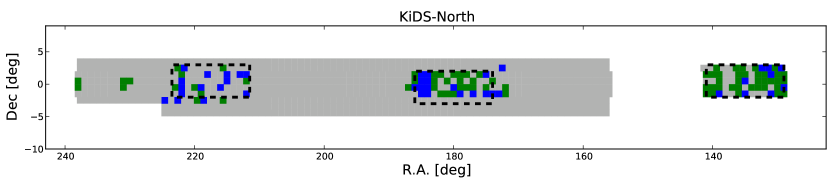
Many other fields have been observed in a subset of the filters and will be included in future releases once their wavelength coverage is complete. Figure 1 shows the sky distribution of the tiles included in KiDS-ESO-DR1/2 within the KiDS fields. A complete list of all tiles with data quality parameters can be found on the KiDS website222http://kids.strw.leidenuniv.nl/DR2.
2.4 Data products
For every tile in the first two data releases of KiDS the following data products are included for each of the bands, , , , and :
-
•
astrometrically and photometrically calibrated, stacked images (“coadds”)
-
•
weight maps
-
•
flag maps (“masks”) that flag saturated pixels, reflection halos, read-out spikes, etc.
-
•
single-band source lists
The multi-band source catalogue encompassing the combined area of the two data releases, although forming one large catalogue, is stored in multiple files, namely one per survey tile.
2.4.1 Coadded image units and gain
The final calibrated, coadded images have a uniform pixel scale of 0.2 arcsec. The pixel units are fluxes relative to the flux corresponding to magnitude = 0. This means that the magnitude corresponding to a pixel value is given by:
| (1) |
The gain varies slightly over the field-of-view because of the photometric homogenization procedure described in Sect. 4.2. An average effective gain is provided online333http://kids.strw.leidenuniv.nl/DR2/data_table.php. An example of a FITS header of a coadded image is also provided online444http://kids.strw.leidenuniv.nl/DR2/example_imageheader.txt.
2.4.2 Single-band source list contents
For each tile single-band source lists are provided for each of the survey filters. To increase the usefulness and versatility of these source lists, an extensive set of magnitude and shape parameters are included, including a large number (27) of aperture magnitudes. The latter allows users to use interpolation methods (e.g. “curve of growth”) to derive their own aperture corrections or total magnitudes. Also provided is a star-galaxy separation parameter and information on the mask regions (see Sect. 4.4) that might affect individual source measurements. Details on the production of these source lists, including source detection and other measurements are discussed in Sect. 4.5.1.
Table LABEL:Tab:singlebandcolumns lists the columns that are present in the single-band source lists provided in KiDS-ESO-DR1/2. Note that of the 27 aperture flux columns only the ones for the smallest aperture (2 pixels, or 0.4″ diameter) and the largest aperture (200 pixels, or 40″ diameter) are listed.
2.4.3 Multi-band catalogue contents
KiDS-ESO-DR2 includes a multi-band source catalogue. This catalogue is based on source detection in the -band images. While magnitudes are measured for all of the filters, the star-galaxy separation, positional, and shape parameters are based on the -band data. The choice of -band is motivated by the fact that it typically has the best image quality and thus provides the most reliable source positions and shapes. Seeing differences between observations in the different filters are mitigated by the inclusion of aperture corrections. Details on the production of this catalogue are discussed Sect. 4.5.2 and Table 8 lists the columns present in the multi-band source lists in KiDS-ESO-DR2.

2.5 Colour terms
The photometric calibration provided in KiDS-ESO-DR1 and KiDS-ESO-DR2 is in AB magnitudes in the instrumental system. Colour-terms have been calculated with respect to the SDSS photometric system.
Aperture-corrected magnitudes taken from the multi-band catalogue were matched to SDSS DR8 (Aihara et al., 2011) PSF magnitudes of point-like sources. For each filter, the median offset to SDSS is first subtracted, rejecting tiles where this offset exceeds 0.1 mag in any of the bands (10 tiles), in order to prevent poor photometric calibration to affect the results. The fit is performed on all points from the remaining tiles. Figure 2 shows the photometric comparison and the following equations give the resulting colour terms:
| (2) | |||
| (3) | |||
| (4) | |||
| (5) |
2.6 Data access
Data from the first two KiDS data releases can be accessed in a number of different ways: through the ESO science archive, from the Astro-WISE archive, or via a web-based synoptic table on the KiDS website555http://kids.strw.leidenuniv.nl/DR2.
2.6.1 ESO archive
As an ESO public survey, the KiDS data releases are distributed via the ESO Science Archive Facility666http://archive.eso.org. Using the Phase 3 query forms users can find and download data products such as the stacked images and source lists.
The naming convention used for all data product files in the ESO archive is the following:
KiDS_DRV.V_R.R_D.D_F_TTT.fits,
where V.V is the data release version, R.R and D.D
are the RA and DEC of the tile center in degrees (J2000.0) with 1
decimal place, F is the filter (, , , , or ),
and TTT is the data product type. Table 1
lists the ESO product category name, file type, value of TTT,
and an example filename for each type of data product.
For example, the KiDS-ESO-DR1 -band stacked image of the tile ”KIDS_48.3_-33.1” is called KiDS_DR1.0_48.3_-33.1_r_sci.fits, and the KiDS-ESO-DR2 multi-band source list data file corresponding to this tile is called KiDS_DR2.0_48.3_-33.1_ugri_src.fits.
| Data product | ESO product category name | File type | TTTa𝑎aa𝑎aTTT is the three character string indicating the data product type. |
|---|---|---|---|
| Calibrated, stacked images | SCIENCE.IMAGE | FITS image | sci |
| Weight maps | ANCILLARY.WEIGHTMAP | FITS image | wei |
| Masks | ANCILLARY.MASK | FITS image | msk |
| Single-band source lists | SCIENCE.SRCTBL | Binary FITS table | src |
| Multi-band catalogue | SCIENCE.SRCTBL | Binary FITS table | src |
2.6.2 Astro-WISE archive
All data products can also be retrieved from the Astro-WISE system (Valentijn et al., 2007; Begeman et al., 2013), the main data processing and management system used for processing KiDS data. The pixel data and source lists are identical to the data stored in the ESO Science Archive Facility, but additionally, the full data lineage is available in Astro-WISE. This makes this access route convenient for those wanting to access the various quality controls or further analyse, process or data-mine the full data set instead of particular tiles of interest.
All data products can be accessed through the links provided on the KiDS website via the DBviewer interface. Downloading of files, viewing inspection plots, and browsing the data lineage is fully supported by the web interface.
2.6.3 Synoptic table
A third gateway to the KiDS data is the synoptic table that is included on the KiDS website. In this table quality information on different data products is combined, often in the form of inspection figures, offering a broad overview of data quality.
3 Observational set-up
The KiDS survey area is split into two fields, KiDS-North and KiDS-South, covering a large range in right ascension so that observations can be made all year round. The fields, each approximately 750 square degrees in size, were chosen to overlap with several large galaxy redshift surveys, principally SDSS, the 2dF Galaxy Redshift Survey (2dFGRS, Colless et al., 2001) and the Galaxy And Mass Assembly (GAMA) survey (Driver et al., 2011). KiDS-North is completely covered by the combination of SDSS and the 2dFGRS, while KiDS-South corresponds to the 2dFGRS south Galactic cap region. Four out of five GAMA fields lie within the KiDS fields. Figure 1 shows the outline of the survey fields.
Each survey tile is observed in the , , , and bands. Exposure times and observing constraints for the four filters are designed to match the atmospheric conditions on Paranal and optimized for the survey’s main scientific goal of weak gravitational lensing. KiDS makes use of queue scheduling, allowing the data requiring the best conditions to be observed whenever these conditions are met. In order to promote building up full wavelength coverage as quickly as possible, pointings for which a subset of filters has been observed receive higher priority. Unfortunately, the queue scheduling system does not allow prioritizing of survey tiles based on the observational progress of neighboring tiles. As a result, the queued tiles are observed in a random order, resulting in the patchy on-sky distribution visible in Fig. 1. The median galaxy redshift of the final survey will reach 0.7 and the best seeing conditions are reserved for the -band, since this functions as the shape measurement band. Each position on the sky is visited only once in each filter, so that the full survey depth is reached immediately. While this precludes variability studies, it will allow the other science projects to benefit from deep data from the start. During the survey the observing constraints have been fine-tuned to optimize between survey speed and scientific return, and Table 2 lists the limits employed for the majority of the period during which the data presented here were obtained.
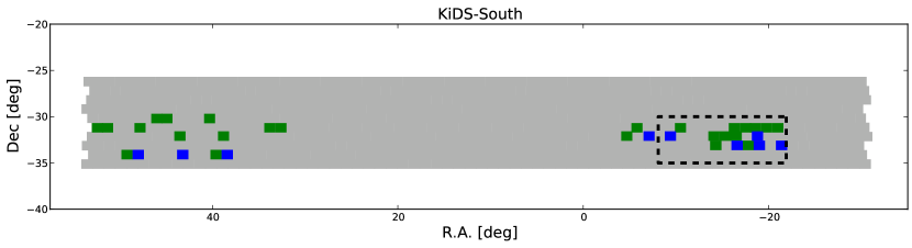
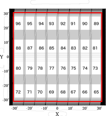
Since the OmegaCAM CCD mosaic consists of 32 individual CCDs, the sky covered by a single exposure is not contiguous but contains gaps. In order to fill in these gaps, KiDS tiles are built up from 5 dithered observations in , and and 4 in . The dithers form a staircase pattern with dither steps of 25″ in X (RA) and 85″ in Y (DEC), bridging the inter-CCD gaps (de Jong et al., 2013), see Fig. 3. Although filled in, the gaps result in areas within the footprint that are covered by fewer than 5 exposures, thus yielding slightly lower sensitivity. Due to this dithering strategy the final footprint of each tile is slightly larger than 1 square degree: arcminutes in ; arcminutes in , and . Neighbouring dithered stacks have an overlap in RA of 5% and in DEC of 10%. The tile centers are based on a tiling strategy that covers the full sky efficiently for VST/OmegaCAM 888http://www.astro.rug.nl/~omegacam/dataReduction/Tilingpaper.html. The combination of the tiling and dithering scheme ensures that every point within the survey area is covered by a minimum of 3 exposures.
| Filter | Max. lunar | Min. moon | Max. seeing | Max. airmass | Sky transp. | Dithers | Total Exp. |
|---|---|---|---|---|---|---|---|
| illumination | distance (deg) | (arcsec) | time (s) | ||||
| 0.4 | 90 | 1.1 | 1.2 | CLEAR | 4 | 1000 | |
| 0.4 | 80 | 0.9 | 1.6 | CLEAR | 5 | 900 | |
| 0.4 | 60 | 0.8 | 1.3 | CLEAR | 5 | 1800 | |
| 1.0 | 60 | 1.1 | 2.0 | CLEAR | 5 | 1200 |
4 Data processing
The data processing pipeline used for KiDS-ESO-DR1/2 is based on the Astro-WISE optical pipeline described in McFarland et al. (2013, henceforth MF13). Below we summarize the processing steps and list KiDS-specific information, covering the KiDS process configuration and departures from the Astro-WISE optical pipeline.
4.1 Image detrending
The first processing steps are the detrending of the raw data, consisting of the following steps.
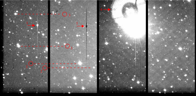
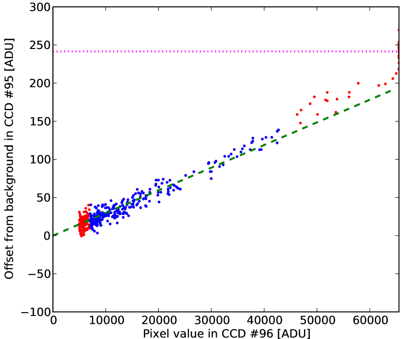
Cross-talk correction. Electronic cross-talk occurs between several CCDs, but most strongly between CCDs #93, #94, #95 and #96, which share the same video board (see Fig. 3 for CCD numbering scheme). Cross-talk can be both positive and negative, resulting in faint imprints of bright sources on neighbouring CCDs (Fig. 4). Although the cross-talk is generally stable, abrupt changes can occur during maintenance or changes to the instrumentation.
A correction is made for cross-talk between CCDs #95 and #96, where it is strongest (up to 0.7%). Crosstalk between a pair (“source” and “target”) of CCDs is determined by measuring for each pixel, with a value greater than 5000 ADU in the source CCD, the offset of the same pixel in the target CCD from the median value of all pixels in the target CCD. A straight line is fit to the trend of this offset as function of the pixel value of the source CCD. See Fig. 5 for an example. The slope of the line () is given in Table 3 per stable period. A separate constant is fit to saturated pixels in the source CCD ( in the table). To correct for the crosstalk between CCDs #95 and #96 the correction factor is applied to each pixel in the target CCD based on the corresponding pixel values in the source CCD:
| (6) |
where and are the pixel values in CCDs and , is the corrected pixel value in CCD due to cross-talk from CCD , and is the saturation pixel value.
| Period | 95 to 96 | 96 to 95 | ||
|---|---|---|---|---|
| () | () | |||
| 2011-08-01 - 2011-09-17 | 210.1 | 2.504 | 59.44 | 0.274 |
| 2011-09-17 - 2011-12-23 | 413.1 | 6.879 | 234.8 | 2.728 |
| 2011-12-23 - 2012-01-05 | 268.0 | 5.153 | 154.3 | 1.225 |
| 2012-01-05 - 2012-07-14 | 499.9 | 7.836 | 248.9 | 3.110 |
| 2012-07-14 - 2012-11-24 | 450.9 | 6.932 | 220.7 | 2.534 |
| 2012-11-24 - 2013-01-09 | 493.1 | 7.231 | 230.3 | 2.722 |
| 2013-01-09 - 2013-01-31 | 554.2 | 7.520 | 211.9 | 2.609 |
| 2013-01-31 - 2013-05-10 | 483.7 | 7.074 | 224.7 | 2.628 |
| 2013-05-10 - 2013-06-24 | 479.1 | 6.979 | 221.1 | 2.638 |
| 2013-06-24 - 2013-07-14 | 570.0 | 7.711 | 228.9 | 2.839 |
| 2013-07-14 - 2014-01-01 | 535.6 | 7.498 | 218.9 | 2.701 |
De-biasing and overscan correction. The detector bias is subtracted from the KiDS data in a two step procedure. First, for each science and calibration exposure the overscan is subtracted per row (no binning of rows). For consistency, all science and calibration data are reduced with this same overscan correction method. Second, a daily overscan-subtracted master bias, constructed from ten bias frames and applying 3 rejection, is subtracted.
Flat-fielding.
A single masterflat (per CCD and filter) was used for all data in the
release. This is by virtue that the intrinsic pixel sensitivities can
be considered constant to or better for , and
(Verdoes Kleijn et al., 2013).
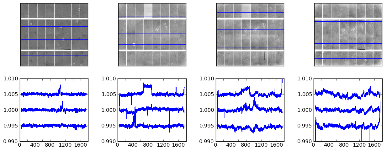
This is illustrated in Fig. 6, where a series of dome flat ratios is shown. The dome flatfields offer the optimal controlled experiment for assessing the pixel sensitivities, as the conditions under which they are observed are closely monitored and calibrated. More specifically,
the calibration unit has a special power supply which allows the ramping of the current when switching on and off and the stabilization of the current during the exposure, delivering an exposure level variation less than 0.6 % over a period of 1 month (Verdoes Kleijn et al., 2013).
The series of ratio plots in Fig. 6 spans the full time period during the KiDS-ESO-DR1/2 observations, demonstrating that the peak-to-valley pixel-to-pixel variations vary less than 0.5% at any time and pixel position.
For , and the master flat is a combination of a master
dome (for high spatial frequencies) and master twilight (=sky)
flat-field (for low spatial frequencies). Both contributing flats are
an average of 5 raw flat-field exposures with 3 rejection. In
band only the twilight flats are used.
Illumination correction. An illumination correction (also known as “photometric superflat”) is required to correct for illumination variations due to stray light in the flat field images, because of which the flat fields are not a correct representation of the pixel sensitivities and vignetting effects. The illumination correction is applied in pixel space, and only on the source fluxes (i.e., after background subtraction). A single illumination correction image is used to correct the single master flats per filter for all data. The correction is determined from observations of several Landolt Selected Area (SA) fields (Landolt, 1992) observed at 33 dither positions, such that the same stars are observed with all CCDs. After computing zero-points per CCD the residuals between the measured stellar magnitudes and their reference values sample the illumination variations. Per CCD the illumination correction is characterized to better than 1%. For further details see Verdoes Kleijn et al. (2013).
De-fringing. De-fringing is only needed for the KiDS -band. Analysis of nightly fringe frames showed that the pattern is constant in time. Therefore, a single fringe image was used for all KiDS-ESO-DR1 images observed after 2012-01-11. For each science exposure this fringe image is scaled and then subtracted to minimize residual fringes. The general procedure, described in MF13, was modified for the KiDS data in order to take large-scale background fluctuations into account. Some -band data contain significant background fluctuations even after flatfielding due to scattered light (see Sect. 5.5), which can cause problems with the scaling of the fringe frame. Therefore, background-subtracted science frames were used to determine the scale factor.
Pixel masking. Cosmic-rays, hot and cold pixels, and saturated pixels are automatically masked as described in MF13 during de-trending. These are included in the weight image. Additional automatic and manual masking is then applied on the coadds as described in Sect. 4.4.
Satellite track removal. Satellite tracks are detected by an automated procedure, working on single CCDs, that applies the Hough transform (Hough, 1962) to a difference image between exposures with the smallest dither offset. Bright stars and bright reflection halos are masked to limit false detections. The pixels affected by satellite tracks are masked and included in the weight image. Due to the single-CCD approach small sections of satellite tracks in CCD corners may be missed by the algorithm. These remnants are included in the manual masks discussed in Sect. 4.4.
Background subtraction. Many observations show darkened regions at the horizontal CCD edges where the bond wire baffling is placed (Iwert et al. 2006). For KiDS-ESO-DR1/2 this CCD-edge vignetting is corrected by performing a line-by-line background subtraction, implemented as a new background subtraction method during regridding (see Sect. 3.5 of MF13).
The line-by-line background subtraction can be inaccurate if there are not enough ‘background’ pixels on a line, for example nearby bright stars. These regions are identified in the masks.
Non-linearity. The linearity of the response of the OmegaCAM detector-amplifier chain is regularly monitored as part of the VST calibration procedures. No significant non-linearities are present (at the level of 1% over the full dynamic range of the system), and the pipeline currently does not include a non-linearity correction step.
4.2 Photometric calibration
The steps taken to calibrate the photometry are as follows. The calibration described here is performed per tile and per filter and applied to the pixel data, which is rescaled to the flux scale in Eq. 1.
-
•
Photometric calibration of the KiDS-ESO-DR1/2 data starts with individual zero-points per CCD based on SA field observations (see MF13 for details of the zero-point derivation). The calibration deploys a fixed aperture of 30 pixels (6.4″ diameter) not corrected for flux losses, and uses SDSS DR8 PSF magnitudes of stars in the SA fields as reference. Zero-points are determined every night, except when no SA field observations are available, in which case default values, that were determined in the same way, are used. The total number of tiles for which these default values were used is 16, 13 and 14 in , and , respectively, or 10% of all tiles. For the nightly zero-point determinations often show large uncertainties and default zero-points are used more frequently, namely in 112 tiles. Magnitudes are expressed in AB in the instrumental photometric system. No colour corrections between the OmegaCAM and SDSS photometric system are applied.
-
•
Next, the photometry in the , and filters is homogenized across CCDs and dithers for each tile independently per filter. For -band this homogenization is not applied because the relatively small source density often provides insufficient information to tie adjacent CCDs together. This global photometric solution is derived and applied in three steps:
-
1.
From the overlapping sources across dithered exposures, photometric differences between the dithers (e.g. due to varying atmospheric extinction) are derived.
-
2.
Although each CCD was calibrated with its own zero-point, the remaining photometric differences between CCDs are calculated using all CCD overlaps between the dithered exposures. The number of sources in these overlaps can range between a few to several hundreds, depending on the filter and the size of the overlap, and a weighting scheme is used based on the number of sources. Both in steps 1 and 2, photometric offsets are obtained by minimizing the difference in source fluxes between exposures and CCDs using the algorithm of Maddox et al. (1990).
-
3.
The offsets are applied to all CCDs with respect to the zero-points valid for the night, derived from the nightly SA field observations.
-
1.
4.3 Astrometric calibration
A global (multi-CCD and multi-dither) astrometric calibration is calculated per filter per tile. SCAMP (Bertin, 2006) is used for this purpose, with a polynomial degree of 2 over the whole mosaic. The (unfiltered) 2MASS-PSC (Skrutskie et al., 2006) is used as astrometric reference catalogue, thus the astrometric reference frame used is International Celestial Reference System (ICRS). Using unwindowed positions the external (i.e. with respect to the 2MASS-PSC) and internal accuracies are typically described by a 2-D RMS of 0.3″and 0.03″, respectively (see also Sect. 5.3). A more detailed description of the astrometric pipeline can be found in MF13.
4.3.1 Regridding and coadding
SWARP (Bertin et al., 2002) is used to resample all exposures in a tile to the same pixel grid, with a pixel size of 0.2″. After an additional background subtraction step (using 33 filtered 128128 pixel blocks) the exposures are scaled to an effective zero-point of 0 (see also Sect. 2.4.1) and coadded using a weighted mean stacking procedure. The applied projection method is Tangential, Conic-Equal-Area. Due to the individual photometric offsets applied to the CCDs the gain varies slightly over the coadd. An average effective gain is calculated for each coadd as:
| (7) |
where and are the median gain and scale factor of the regridded CCD images and is the number of exposures. These average gain values are provided in the online Data table999http://kids.strw.leidenuniv.nl/DR2.
4.4 Masking of bright stars and defects
Nearby saturated stars and other image defects are the main source of contamination in the measurement of objects. In KiDS coadds, these features are masked by a stand-alone program, Pulecenella (v1.0, Huang et al. in prep). Pulecenella is a novel procedure for automated mask creation completely independent of external star catalogues. An example of a mask image is shown in Fig. 7.
Pulecenella detects and classifies the following types of image artifacts resulting from the saturated stars:
-
–
saturated pixels in the core and vicinity of stars,
-
–
spikes caused by diffraction of the mirror supports,
-
–
spikes caused by readout of saturated pixels,
-
–
“ghost” halos produced by the reflections off of optics (up to three wider reflection halos with spatially dependent offsets; these are caused by reflections of different optical elements in the light-path and depend on the brightness of the star).
These features have regular shapes, and scale with the brightness and position of bright stars in a stable way in all images in a given observation band. Hence, Pulecenella is first configured to model the mask shapes (including the radius of saturation cores, the orientation of diffraction spikes, the size and offset of reflection halos) from some sampled saturated stars; the so configured analytical models are then applied to the batch masking of coadds from the same band. The detection, location and magnitude of saturated stars are derived from a first SExtractor (Bertin & Arnouts, 1996) run over the image to be masked, with a band-specific configuration aiming only for the detection and measurement of the nearly saturated stars; the saturation pixel level is derived from the FITS image header. Thus, Pulecenella produces star masks specifically for each image, without any dependence on an external star catalogue. This also avoids the ambiguity in the determination of the magnitude cutoff of saturated stars due to the difference between the observed and external catalogue filters.
The position of reflection halos is offset from the center of the host saturated star; the offset can be towards or outward from the image center, depending on the reflection components in the optics. For the primary reflection halo, the offset is first linearly modeled from several primary halos of the brightest stars in the image, and whether the halo mask is applied depends on the brightness of the saturated stars; this brightness level is determined as the number of pixels for which the count level exceeds 80% of the saturation limit and is therefore independent of the photometric calibration. The same method is applied for secondary and tertiary halos independently. The details of the masking method are presented in Huang et al. (2015, in prep).
Besides the analytical star masks, Pulecenella is also configured to mask pixels in the empty boundary margins, CCD gaps or dead pixels with zero weight. These pixels are flagged as ’bad pixels’. Finally, bad regions which are missed by Pulecenella (e.g. large-scale background artifacts) but are detected by a visual inspection, are manually masked using DS9 and added both to the region file and to the final flag image.
As output, Pulecenella generates both an ASCII mask region file which is compatible with the DS9101010http://ds9.si.edu tool and a FITS flag image that can be used in SExtractor. Different types of masked artifacts/regions are coded with the different binary values listed in Table 4. In the flag image these binary values are summed.
The flag image is used during source extraction for the single-band source list (see below) to flag sources whose isophotes overlap with the critical areas. The resulting flags are stored in the following two SExtractor parameters:
-
–
IMAFLAGSISO: sum of all mask flags encountered in the isophote profile,
-
–
NIMAFLAGISO: number of flagged pixels entering IMAFLAGSISO.
| Type of area | Flag | Type of area | Flag |
|---|---|---|---|
| Readout spike | 1 | Secondary halo | 16 |
| Saturation core | 2 | Tertiary halo | 32 |
| Diffraction spike | 4 | Bad pixel | 64 |
| Primary halo | 8 | Manually masked | 128 |
Table 5 summarizes the percentages of the total area in KiDS-ESO-DR1/2 that are not masked, masked automatically by Pulecenella, and manually masked. Due to the lower sensitivity in the number of saturated stars is much smaller, leading to a significantly smaller percentage of masked pixels. The high fraction of area that is manually masked in -band is due to the higher frequency and severity of scattered light issues (see Sect. 5.5) caused by moonlight and higher sky brightness. Taking into account the nominal area covered by KiDS-ESO-DR1/2 the total unmasked area is approximately 120 square degrees.
| Filter | Not masked | Automatically | Manually |
|---|---|---|---|
| masked | masked | ||
| 97 | 1 | 2 | |
| 86 | 7 | 7 | |
| 78 | 12 | 10 | |
| 77 | 9 | 14 |
4.5 Source extraction and star/galaxy separation
Single-band source lists were included in KiDS-ESO-DR1, while KiDS-ESO-DR2 contains both single-band source lists, as well as a multi-band source catalogue encompassing the combined area. The single-band source lists are provided per survey tile, while the catalogue, although split into files corresponding to single tiles, is constructed as a single catalogue. Both the source lists and the catalogue are intended as “general purpose” catalogues.
4.5.1 Single-band source lists
| Parameter | Value | Description |
|---|---|---|
| DETECT_THRESH | 1.5 | ¡sigmas¿ or ¡threshold¿,¡ZP¿ in mag/arcsec2 |
| DETECT_MINAREA | 3 | minimum number of pixels above threshold |
| ANALYSIS_THRESH | 1.5 | ¡sigmas¿ or ¡threshold¿,¡ZP¿ in mag/arcsec2 |
| DEBLEND_NTHRESH | 32 | Number of deblending sub-thresholds |
| DEBLEND_MINCONT | 0.001 | Minimum contrast parameter for deblending |
| FILTER | Y | Apply filter for detection (Y or N) |
| FILTER_NAME | default.conv | Name of the file containing the filter |
| CLEAN | Y | Clean spurious detections? (Y or N) |
| CLEAN_PARAM | 1.0 | Cleaning efficiency |
| BACK_SIZE | 256 | Background mesh: ¡size¿ or ¡width¿,¡height¿ |
| BACK_FILTERSIZE | 3 | Background filter: ¡size¿ or ¡width¿,¡height¿ |
| BACKPHOTO_TYPE | LOCAL | can be GLOBAL or LOCAL |
| BACKPHOTO_THICK | 24 | thickness of the background LOCAL annulus |
Source list extraction and star/galaxy (hereafter S/G) separation is achieved with an automated stand-alone procedure optimized for KiDS data: KiDS-CAT. This procedure, the backbone of which is formed by SExtractor, performs the following steps separately for each filter.
-
1.
SExtractor is run on the stacked image to measure the FWHM of all sources. High-confidence star candidates are then identified based on a number of criteria including signal-to-noise ratio (SNR) and ellipticity cuts (for details see La Barbera et al., 2008).
-
2.
The average PSF FWHM is calculated by applying the bi-weight location estimator to the FWHM distribution of the high-confidence star candidates.
-
3.
A second pass of SExtractor is run with SEEING_FWHM set to the derived average PSF FWHM. During this second pass the image is background-subtracted, filtered and thresholded “on the fly”. Detected sources are then de-blended, cleaned, photometered, and classified. A number of SExtractor input parameters are set individually for each image (e.g., SEEING_FWHM and GAIN), while others have been optimized to provide the best compromise between completeness and spurious detections (see Data Quality section below). The detection set-up used is summarized in Table 6; a full SExtractor configuration file is available online111111http://kids.strw.leidenuniv.nl/DR1/example_config.sex. Apart from isophotal magnitudes and Kron-like elliptical aperture magnitudes, a large number of aperture fluxes are included in the source lists. This allows users to estimate aperture corrections and total source magnitudes. All parameters provided in the source lists are listed in the Data Format section below.
-
4.
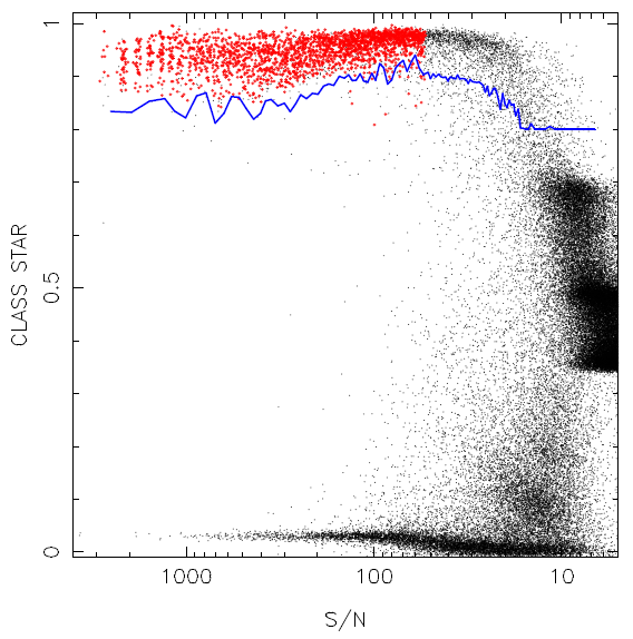
S/G separation is performed based on the CLASS_STAR (star classification) and SNR (signal-to-noise ratio) parameters provided by SExtractor and consists of the following steps:
-
•
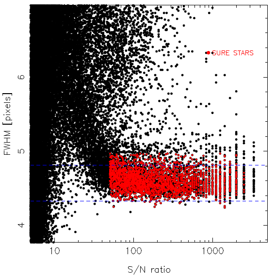
In the SNR range where the high-confidence star candidates are located (the red dots in Fig. 8) the bi-weight estimator is used to define their CLASS_STAR location, , and its width, ; a lower envelope of is defined.
-
•
At SNR below that of the high-confidence star candidates, a running median CLASS_STAR value is computed based on all sources with CLASS_STAR ¿ 0.8. This running median is shifted downwards to match the locus. The resulting curve (blue curve in Fig. 8) defines the separation of stars and galaxies.
-
•
The source magnitudes and fluxes in the final source lists are for zero airmass, but not corrected for Galactic foreground or intergalactic extinction. The result of the S/G classification is available in the source lists via the 2DPHOT flag. Flag values are: 1 (high-confidence star candidates), 2 (objects with FWHM smaller than stars in the stellar locus, e.g., some cosmic-rays and/or other unreliable sources), 4 (stars according to S/G separation), and 0 otherwise (galaxies); flag values are summed, so 2DPHOT = 5 signifies a high-confidence star candidate that is also above the S/G separation line. Table LABEL:Tab:singlebandcolumns lists all columns present in these source lists.
4.5.2 Multi-band catalogue
The multi-band catalogue delivered as part of KiDS-ESO-DR2 is intended as a ”general purpose” catalogue and relies on the double-image mode of SExtractor and also incorporates information obtained using the KiDS-CAT software described above. SExtractor is run four times for each tile, using the , , and KiDS-ESO-DR1/2 coadds as measurement images, to extract source fluxes in each of the filters. The -band coadd is used as detection image in all runs, since it provides the highest image-quality in almost all cases. For the same reason, several shape measurements are based only on the -band data. In the future, it is foreseen that the catalogue S/G separation will make use of colour information and/or PSF modeling. Currently the S/G separation information included in the catalogue is the same as in the -band source list. The detection set-up is identical to that employed for the source detection for the single-band source list (Table 6). Masking information is provided for all filters in the same fashion as in the single-band source lists. Compared to the single-band source lists the number of measured parameters is reduced. Table 8 lists the columns present in these source lists.
To account for seeing differences between filters aperture corrected fluxes are provided in the catalogue. The aperture corrections were calculated for each filter by comparing the aperture fluxes with the flux in a 30 pixel aperture, the aperture used for photometric calibration, and the aperture-corrected fluxes are included in the catalogue as separate columns. Source magnitudes and fluxes are not corrected for Galactic foreground or intergalactic extinction.
In order to prevent sources in tile overlaps to appear as multiple entries in the catalogue, the survey tiles have been cropped and connect seamlessly to one another. This results in slightly shallower data along the edges of the tiles (Fig. 3), similar to the areas partially covered by CCD gaps. Overall, all included areas are covered by at least three exposures. In future releases this will be improved by combining information from multiple tiles in overlap regions.
5 Data quality
5.1 Intrinsic data quality
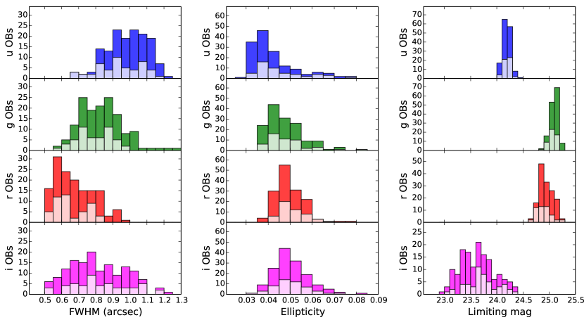
In Fig. 9 the obtained seeing (FWHM), PSF ellipticity, and limiting magnitude distributions per filter are shown, to illustrate the raw data quality. The PSF ellipticity is defined here as , where and are the semi-major and semi-minor axis, respectively. Limiting magnitudes are 5 AB in a 2″ aperture and determined by a fit to the median SNR, estimated by 1/MAGERR_AUTO, as function of magnitude. In case of the filters observed in dark time (, , ) the FWHM distributions reflect the different observing constraints, with -band taking the best conditions. Since -band is the only filter in which the data are obtained in bright time, it is observed under a large range of seeing conditions. Average PSF ellipticities are always small: (the average is over the absolute value of ellipticity, regardless of the direction of ellipticity). The wide range of limiting magnitudes in -band is caused by the large range in moon phase and thus sky brightness.
5.1.1 Point-spread-function
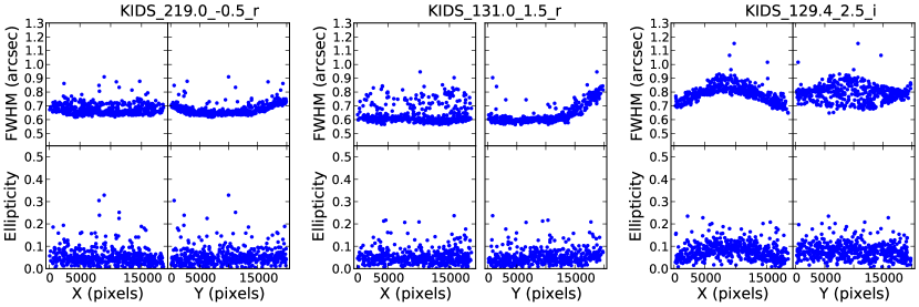
Designed with optimal image quality over the full square degree field-of-view in mind, the VST/OmegaCAM system is capable of delivering images with an extremely uniform PSF. A typical example of the PSF ellipticity and size pattern for an observation taken with a nominal system set-up is shown in the left panel of Fig. 10. Of course, as must be expected from a newly commissioned instrument, the set-up of the optical system is not always perfect and different imperfections can lead to a variety of deviations from a stable and round PSF. Most commonly encountered patterns are related to imperfect focus (increased PSF size either on the outside or on the inside of the FOV) and mis-alignment of the secondary mirror (increased PSF size and ellipticity along one edge of the FOV).
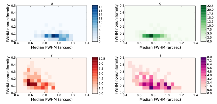
To quantify the stability of the PSF we calculate a PSF size and ellipticity for every observation based on the PSF sizes in 32 regions in the coadded image that correspond roughly to the 32 CCDs. Systematic variations in ellipticity are usually less clear than in PSF size (see Fig. 10), which is why the latter is used for monitoring PSF stability. The average PSF size in the 4 regions with the smallest PSF is subtracted from the average PSF size in the 4 regions with the largest PSF, and the result divided by the average PSF size of the whole image. The distribution per filter of this PSF size nonuniformity is shown versus the median FWHM in Fig. 11. As the median PSF size (i.e. the seeing) increases, the nonuniformity drops, as any differences due to optical imperfections are smoothed out. However, even during very good seeing conditions the PSF size variation rarely exceeds 25% and in most cases is around 10%.
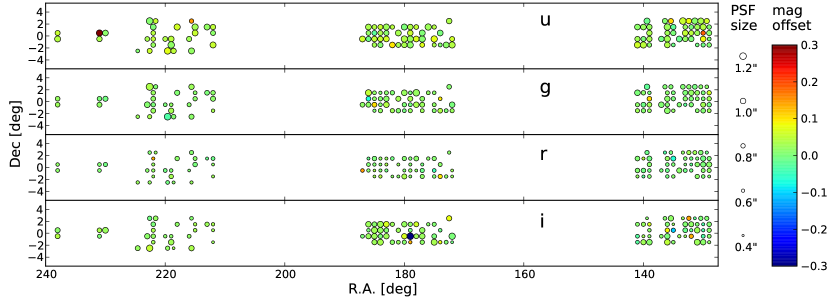
The median PSF sizes for all tiles in the KiDS-North field are indicated in Fig. 12. Both in KiDS-North and KiDS-South there are no systematic gradients in PSF size over the survey area.
5.2 Photometric quality
The matter of photometric quality can be divided in two parts, namely the uniformity of the photometry within each tile, and the quality of the photometric calibration per tile/filter. Since the distribution of tiles included in KiDS-ESO-DR1/2 is not contiguous, with many isolated tiles, a complete photometric homogenization of the entire data set is impossible, and the photometric calibration is currently done per tile and per filter. The quality of the photometry will improve greatly in future releases when, using significant contiguous areas, a global calibration for the entire survey will be performed.
5.2.1 Comparison to SDSS
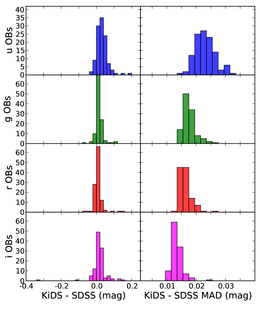
Both the internal photometric homogeneity within a coadd and the quality of the absolute photometric scale is assessed by comparing the KiDS photometry to SDSS DR8 (Aihara et al., 2011), which is photometrically stable to 1% (Padmanabhan et al., 2008). For this purpose, the aperture-corrected magnitudes in the multi-band catalogue were compared to PSF magnitudes of stars in SDSS DR8. Only unmasked stars with photometric uncertainties in both KiDS and SDSS smaller than 0.02 mag in , , and or 0.03 mag in were used. This comparison is only possible for all tiles in the KiDS-North field, but since KiDS-South was calibrated in the same way as KiDS-North, we expect the conclusions to hold for all data.
The consistency of the photometric calibration is illustrated in Fig. 13, where histograms of the distributions of photometric offsets between KiDS and SDSS are shown for the overlapping tiles in KiDS-North. A systematic offset of mag is present in all filters, possibly due to the fact that nightly zero-points are determined using a fixed aperture on stars in the SA field without aperture correction. The scatter and occasional outliers are due to non-photometric conditions (during either KiDS or SA field observations) and, particularly in case of the -band, use of default zero-points. In Fig. 12 the photometric offsets are plotted as function of RA and DEC, demonstrating that there are no large-scale gradients present. All photometric offsets determined from this comparison with SDSS are available in the Source catalogue table on the KiDS website121212http://kids.strw.leidenuniv.nl/DR2.
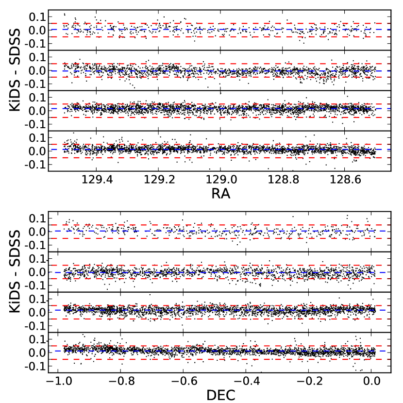
Figure 14 shows the residuals between KiDS and SDSS DR8 magnitudes for one tile (KIDS_129.0_-0.5), which is a representative example. Generally speaking, the photometry in a filter within one tile is uniform to a few percent. The right column of the left panel in Fig. 13 shows the distribution of the Median Absolute Deviation (MAD) of the stellar photometry between KiDS and SDSS for the tiles in KiDS-North, demonstrating the photometric stability within survey tiles. The relatively poor photometry in -band is due to the lack of photometric homogenization within a tile.

5.2.2 Stellar locus
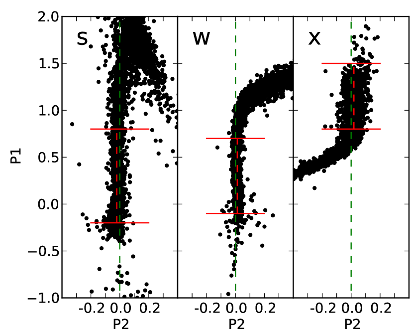
A second quality assessment of the photometry is done by comparing stellar photometry to empirical stellar loci, in the form of the ”principal colours” as defined by Ivezić et al. (2004) based on SDSS photometry. Only unmasked and unflagged stars with ¡21 are used for this analysis. Although small colour terms exist between KiDS and SDSS the stellar loci based on SDSS are a powerful tool to verify the photometric stability over the currently released tiles. Once more complete sky coverage allows an overall photometric calibration of the KiDS data, accurate stellar loci in the KiDS filters will be derived.
Figure 15 shows the stellar locus for the tile KIDS_129.0_-0.5 in the three principal colour planes. These colour planes are different combinations of the filters and denoted by , and . The median colours are calculated for each of , and by choosing all stars within the indicated limits and after clipping all stars more than 200 mmag away from the initial median colour. In Fig. 16 the distributions of the median principal colours are shown, together with the typical width of the stellar locus, measured by the standard deviation. The narrow distributions indicate that the colour of the stellar locus is typically stable to within 20 mmag. Also the stellar locus width is always stable to within 10 mmag. The large width of the stellar locus in is caused by the fact that this part of the locus is made up of relatively faint stars with large photometric uncertainties.
In this analysis three tiles stand out that have a median colour of ¿100 mmag. Comparing these with the SDSS photometry as discussed above shows that one corresponds to the tile with the largest offset (0.32 mag) in and two correspond to tiles with large offsets (¿0.1 mag) in .
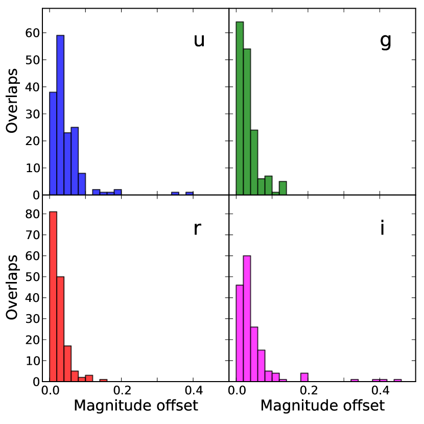
5.2.3 Tile overlaps
Finally, we analyze the tile-to-tile photometric offsets directly from the KiDS data, using the overlapping areas between the tiles where available. This is done per filter, and only stars with a magnitude brighter than 22 in the respective filter are matched. In this results in a total number of sources per overlap region varying between 20 and 300, in and between 50 and 600 and in between 100 and 1,000. In some cases the PSF deteriorates at the edge of a tile, as described Sect. 5.1.1, and the aperture-corrected magnitudes may be affected. For this reason MAG_ISO magnitudes are used for this overlap analysis. The distributions of magnitude offsets in each filter, as determined from the tile overlaps, are shown in Fig. 17. In the filters the offsets are typicaly 0.02 mag, and for this increases to typically 0.04 mag. Taking into account that the photometry in the tile edges is of slightly poorer quality than in the center, due to the fact that these data are less deep, these values are in good agreement with the photometric comparison to SDSS.
5.3 Astrometric quality
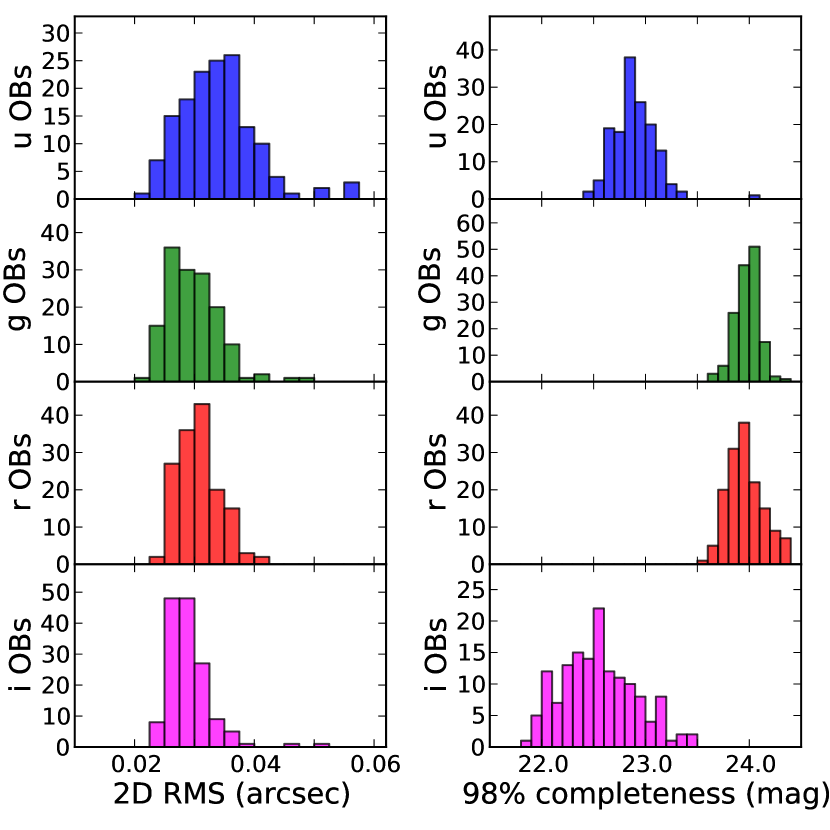
The accuracy of the absolute astrometry (”KiDS vs 2MASS”) is uniform over a coadd, with typical 2-dimensional (2-D) RMS of 0.31″ in , , and , and 0.25″ in , in line with expectations based on the fact that the majority of reference stars used is relatively faint. The lower RMS in -band is most likely due to the fact that in this band on average brighter 2MASS sources are selected as reference sources. The accuracy of the relative astrometry (”KiDS vs KiDS”), measured by the 2-D positional residuals of sources between dithers, is also uniform across a single coadd. In Fig. 18 the accuracy of this relative astrometry of all coadds is shown. The typical 2-D RMS is ″ in all filters, but with a larger scatter in due to the smaller number of available reference sources.
5.4 Completeness and contamination
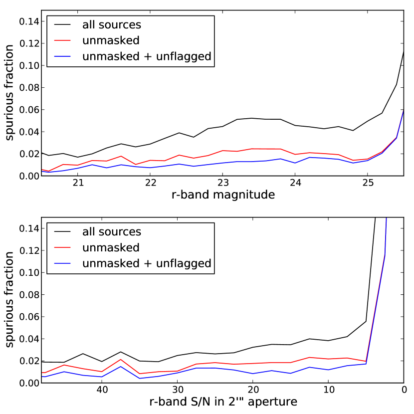
Contamination of the multi-band catalogue by spurious sources was analyzed by means of a comparison of the overlap between KiDS and the CFHT Legacy Survey131313http://www.cfht.hawaii.edu/Science/CFHTLS/, the main deeper survey overlapping with the current data releases (CFHTLS-W2, using their final data release T0007141414http://terapix.iap.fr/cplt/T0007/doc/T0007-doc.html). For the analysis it is assumed that all KiDS sources not detected in CFHTLS-W2 are spurious. Since some fraction of real sources might be absent in the CFHTLS catalogues, the spurious fractions derived should be considered upper limits.
Figure 19 shows the spurious fractions derived from this comparison as function of magnitude (-band MAG_ISO) and signal-to-noise (in a 2″ aperture). When all sources in the catalogue are considered the fraction of spurious sources is estimated to be ¡5% down to a very low SNR of within a 2″ aperture. Filtering sources based on masking information reduces this fraction to , demonstrating that caution is required when using faint sources in masked regions. When sources are filtered both on masking information as well as SExtractor detection flags, the spurious fractions drops even further to , yielding a very clean catalogue down to the detection limit.
An internal estimate of the completeness for the KiDS data is provided per tile, based on the method of Garilli et al. (1999). It determines the magnitude at which objects start to be lost in the source list because they are below the brightness threshold in the detection cell. The implementation is similar to La Barbera et al. (2010). Estimates of the completeness obtained by comparison to deeper CFHTLS-W2 data are consistent with these internally derived values. The distributions of the 98% completeness magnitudes for all tiles are shown in Fig. 18. Comparison with Fig. 9 shows that the 98% completeness limits are typically magnitude brighter than the limiting magnitude for , and and magnitudes brighter in . For the completeness of the multi-band catalogue the values for the -band of each tile apply.
5.5 Data foibles
5.5.1 Scattered light and reflections
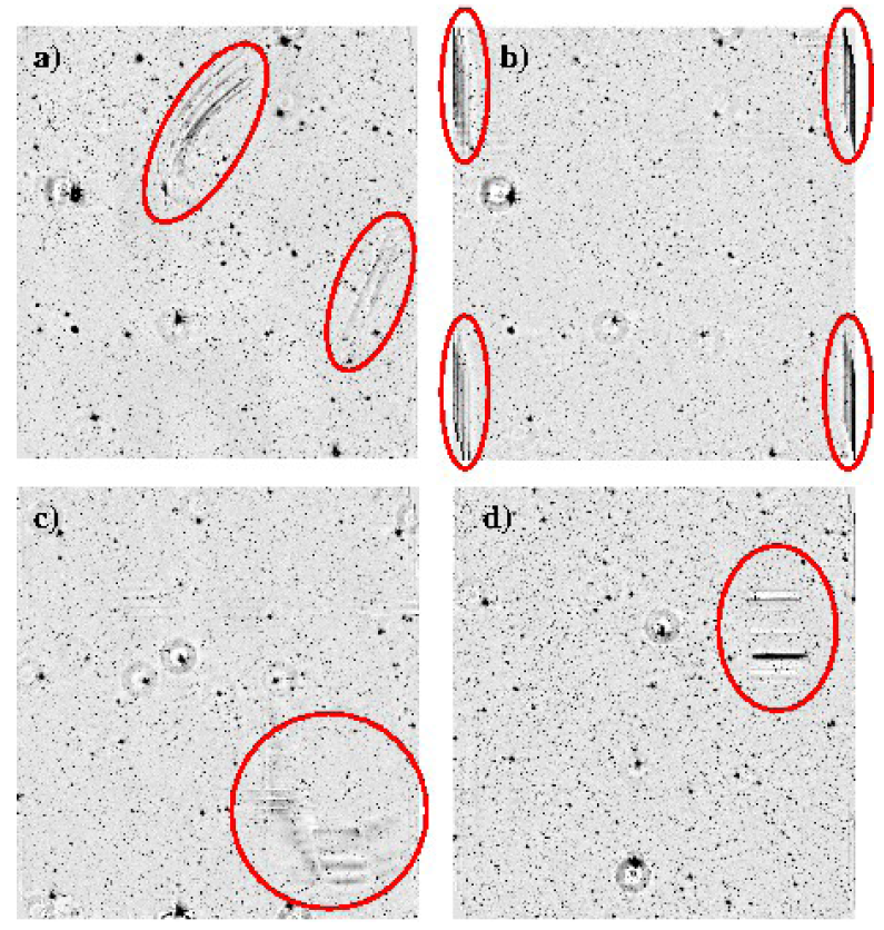
Some of the main challenges in the analysis of early VST/OmegaCAM data are related to scattered light and reflections. Due to the open structure of the telescope, light from sources outside the field-of-view often affects the observations. This expresses itself in a number of ways:
-
•
reflections: in some cases strong reflected light patterns are seen in the focal plane; these are caused by light from bright point sources outside the field-of-view and can occur in all filters. Some examples are shown in Fig. 20a.
-
•
vignetting by CCD masks: vignetting and scattering by the masks present at the corners of the focal plane array, and at the gaps between the rows of CCDs; this effect is particularly strong in i-band due to the bright observing conditions. The effect near the CCD gaps is largely corrected for, but in many cases the areas in the corners of the CCD array is strongly affected. Examples are shown in Fig. 20b.
-
•
extended background artifacts: related to the reflections mentioned before, this is mostly seen in i-band and probably caused by moonlight. An example is shown in Fig. 20c. Most of these effects are not (yet) corrected for in the current data processing, but strongly affected regions are included in the image masks and affected sources are flagged in the source lists and catalogue.
Improvements to the telescope baffles that were installed in early 2014 significantly improve scattered light suppression.
5.5.2 Individual CCD issues
There are two issues related to individual CCDs that noticeably affect this data delivery:
-
•
CCD 82: this CCD suffered from random gain jumps and related artifacts until its video board was replaced on June 2 2012. Artefacts as shown in Fig. 20d are sometimes visible in the image stacks due to this problem. Photometry in this CCD can be used due to the cross-calibration with neighbouring CCDs in the dithered exposures, but part of the CCD is lost. These features are included in the image masks and affected sources are flagged.
-
•
CCD 93: during a few nights in September 2011 (Early Science Time) one CCD was effectively dead due to a video cable problem. One observation included in this data delivery does not include this CCD: the -band observation of KIDS_341.2_-32.1.
6 First scientific applications
The Kilo-Degree Survey was designed for the central science case of mapping the large-scale matter distribution in the Universe through weak gravitational lensing and photometric redshifts. Several other science cases were also identified from the early design stages including studying the structure of galaxy halos, the evolution of galaxies and galaxy clusters, the stellar halo of the Milky Way, and searching for rare objects such as high-redshift QSOs and strong gravitational lenses. While for the main science goal of KiDS the full survey area is required, scientific analyses focusing on the other science cases are currently already on-going. Below we demonstrate the quality and promise of KiDS by means of these on-going research efforts.
6.1 Photometric redshifts and weak gravitational lensing
An analysis of the weak gravitational lensing masses of galaxies and groups in the KiDS images is one of the main early scientific goals of the survey (Viola et al., 2015; van Uitert et al., 2015; Sifón et al., 2015). Such an analysis requires two types of measurements from the KiDS data: galaxy shapes for shear measurements, and galaxy colours for photometric redshifts. The shapes are measured with a dedicated pipeline based on the CFHTLenS analysis (Heymans et al., 2012; Erben et al., 2013; Miller et al., 2013) that combines information from individual exposures and avoids regridding of the pixels to maintain image fidelity as much as possible. The colours and photometric redshifts are derived from the BPZ code (Benítez, 2000; Coe et al., 2006) applied to the output from a PSF-homogenized photometry pipeline — again an evolution from the CFHTLenS analysis pipeline, see Hildebrandt et al. (2012) — which runs on the calibrated stacked images released in KiDS-ESO-DR1/2. Further details of these dedicated analyses are presented in Kuijken et al. (2015).
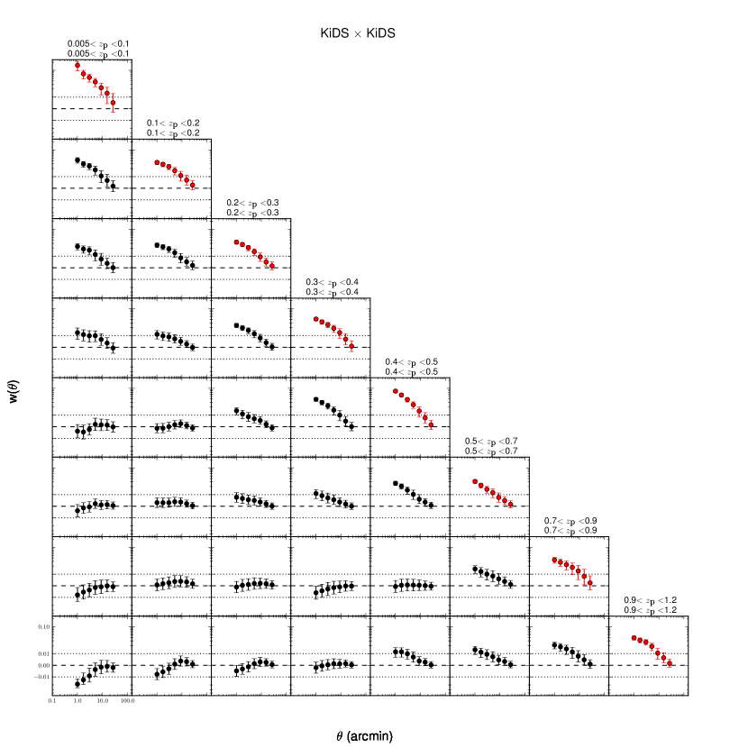
As an illustration of the quality of the photometric redshifts, in Fig. 21 we show the angular cross-correlations of the positions of galaxies in different photometric redshift bins, on scales between 1 and 30 arcminutes (Erben et al., 2009; Benjamin et al., 2010). We use Athena (Kilbinger et al., 2014) to calculate w() using the Landy & Szalay (1993) estimator. Errors are obtained from jackknife resampling, with each pointing being a jackknife sub-sample. The figure shows a clear clustering signal of galaxies within the same redshift bin (panels on the diagonal). Most off-diagonal panels show a smaller cross-correlation amplitude than the corresponding auto-correlations, and mostly this signal is seen only between neighbouring redshift bins, as would be caused by scatter of the photometric redshift estimates into neighbouring bins. The fact that no strong signal is seen further away from the diagonal shows that the level of catastrophic failures in the redshifts is low, and provides confidence in the photometric redshifts as well as the underlying photometry reported here.
This photometric redshift-only cross-correlation check is complementary to the spectroscopic redshift-photometric redshift cross-correlations presented in Kuijken et al. (2015). The latter analysis has the advantage of utilising spectroscopic redshifts, which provide a better representation of the ’absolute truth’; however, the spectroscopic redshifts only reach up to , so there is additional information provided by the photometric redshift-only cross-correlations out to . We refer the interested reader to Kuijken et al. (2015) for details of the cross-correlation analysis between the photometric redshifts and the available spectroscopic redshifts.
6.2 Photometric redshifts from machine learning
Apart from the photometric redshifts described in Sect. 6.1, photometric redshifts are also derived from KiDS-ESO-DR1/2 photometry using the supervised machine learning model MLPQNA: a Multi-Layer Perceptron feed-forward neural network providing a general framework for representing nonlinear functional mappings between input and output variables. QNA stands for Quasi Newton Algorithm, a variable metric method used to solve optimization problems (Davidon, 1991) that, when implemented as the learning rule of a MLP, can be used to find the stationary (i.e. the zero gradient) point of the learning function. The QNA implemented here is the L-BFGS algorithm from Shanno (1970). Supervised methods use an extensive set (the knowledge base or KB) of objects for which the output (in this case the redshift) is known a-priori to learn the mapping function that transforms the input data (in this case the photometric quantities) into the desired output. Usually the KB is split into three different subsets: a training set for training the method, a validation set for validating the training in particular against overfitting, and a test set for evaluating the overall performance of the model (Cavuoti et al., 2012; Brescia et al., 2013). In the method used here the validation is embedded into the training phase, by means of the standard leave-one-out k-fold cross validation mechanism (Geisser, 1975). Performances are always derived blindly, i.e. using a test set formed by objects which have never been fed to the network during either training or validation. The MLPQNA method has been successfully used in many experiments on different data sets, often composed through accurate cross-matching among public surveys (SDSS for galaxies: Brescia et al. 2014; UKIDSS, SDSS, GALEX and WISE for quasars: Brescia et al. 2013; CLASH-VLT data for galaxies: Biviano et al. 2013).
The KB of spectroscopic redshifts was obtained by merging the spectroscopic datasets from GAMA data release 2 (Liske et al., 2014) and SDSS-III data release 9 (Ahn et al., 2012), while for the KiDS photometry two different aperture magnitudes were adopted. The final KB includes the optical magnitudes () within 4″and 6″diameters and SDSS and GAMA heliocentric spectroscopic redshifts. GAMA redshifts come with the normalized quality flag NQ.
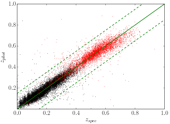
A training set and a test set were created by splitting the KB into two parts of 60% and 40%, respectively. With these data sets two experiments were performed, one using only the GAMA high-quality (HQ, ) spectroscopic redshifts and one using a mix of GAMA and SDSS spectroscopic information. These experiments are illustrated in Fig. 22. To quantify the quality of the results we use the standard normalized photometric redshift error defined as . We find a scatter in of 0.027 and 0.031 and a fraction of catastrophic outliers () of 0.25% and 0.39% for the high-quality GAMA and the GAMA+SDSS spectroscopic data sets, respectively. The mixture of GAMA HQ + SDSS spectroscopic data slightly extends the KB to higher redshifts, but since there is still very limited information at , this does not significantly increase the performance at higher redshift. Finally, the presence of objects at the minimum indicates a residual presence of stars within the sample. Further information about the experiments, results and the produced catalogue of photometric redshifts is reported in Cavuoti et al. (2015). A detailed comparison with redshifts from SED-fitting will be presented in a forthcoming paper (Cavuoti et al. in preparation).
6.3 Galaxy structural parameters and scaling relations
Galaxies are the building blocks of the Universe and within the framework of hierarchical structure formation they form bottom-up, with smaller objects forming first, then merging into massive structures (e.g. De Lucia et al. 2006; Trujillo et al. 2006). However, high-mass galaxies seem to have formed most of their stars in earlier epochs and over a shorter time interval than the lower mass ones (“downsizing” scenario, Fontanot et al. 2009). Characterising the properties of the luminous matter and the way this has been assembled into dark-matter haloes is crucial to reconcile theory and observations. Making use of the high spatial resolution, depth and area coverage of KiDS we aim to measure, across different redshift slices:
-
•
total luminosity and the stellar mass through SED fitting (e.g. Le PHARE, Arnouts et al. 1999);
-
•
stellar population properties (Bruzual & Charlot 2003);
-
•
structural parameters and colour gradients.
This will be one of the first samples of this depth over such a large area and wavelength coverage, allowing us to extend previous analyses (e.g. La Barbera et al. 2010) to higher redshifts.
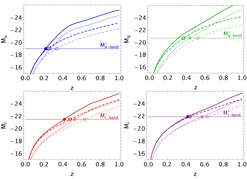
From the KiDS-ESO-DR1/2 catalogues we select galaxies based on the S/G separation discussed in Sect. 4.5 with additional selection criteria on size (to further reduce contamination by stars), and remove any flagged or masked objects. For KiDS-ESO-DR1/2 this results in a sample of million galaxies. For million of these we have measured photometric redshifts as discussed in Sect. 6.2. For the structural parameter derivation we have considered only galaxies with high -band SNR (SNR) to reliably perform the surface brightness analysis (La Barbera et al. 2008, 2010). This sub-sample consists of around 350,000 galaxies. The completeness of the whole sample has been discussed in Sect. 5.4. For the sample with photometric redshifts the 98% completeness magnitudes (all magnitudes used here are MAG_AUTO) are =22.3, =22.1, =20.4 and =19.7, which correspond to 90% completeness magnitudes of =23.1, =23.0, =22.1 and =21.2. The stringent cuts on SNR for the sample with structural parameters results in 98% completeness magnitudes of =21.4, =21.1, =20.1, =19.3 and 90% completeness magnitudes of =22.2, =21.7, =21.0, =20.2. These completeness magnitudes can be converted to absolute magnitudes as , where is the distance modulus based on the photometric redshift and is the K-correction, which is derived for two empirical models (elliptical and Scd galaxy). For these calculations a standard cosmology with , and km s-1 Mpc-1 is used, and the galactic foreground extinction is corrected based on the dust maps from Schlegel et al. (1998). Figure 23 shows how the 90% completeness limits vary with absolute magnitude as a function of redshift. Comparing this to the from the luminosity function of low- SDSS galaxies (Blanton et al. 2005) we find that is reached at 0.22, 0.31, 0.42, and 0.42 in our high-SNR galaxy sample and 0.27, 0.44, 0.53, and 0.57 for the photo-z sample, in , , and , respectively, if the Elliptical model is adopted. Slightly larger redshifts are found for late-type galaxies (see Fig. 23).
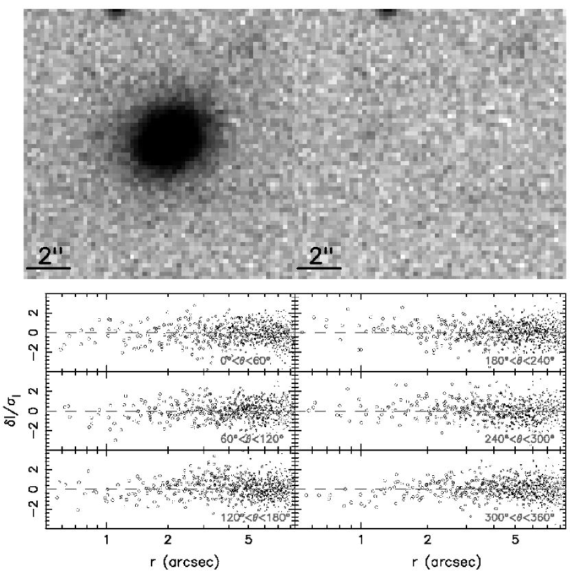
We make use of Galfit (Peng et al. 2010) and 2DPHOT (La Barbera et al. 2008) to fit PSF convolved Sérsic profiles to the surface photometry and infer the structural parameters (Sérsic index, , effective radius , axial ratio, , disky/boxy coefficient , disk/bulge separation). In Fig. 24 we show an example of the results obtained with 2DPHOT. The relationship between or Sérsic index and mass, luminosity and its evolution with redshift has been demonstrated to be a fundamental probe of galaxy evolution and the role of mass accretion in galaxy merging (Trujillo et al. 2007; Hilz et al. 2013; Tortora et al. 2014). This characterization of 2D light profiles also allows one to determine the colour gradients (La Barbera & de Carvalho 2009; Tortora et al. 2010a; Tortora et al. 2011a; La Barbera et al. 2011; Tortora & Napolitano 2012; La Barbera et al. 2012), which can be compared to simulations (e.g.Tortora et al. 2011b; Tortora et al. 2013).
The resulting data set is introduced in Tortora et al. (2015) and applied to a first census of compact galaxies, a special class of objects, relic remnants of high-z red nuggets, which can provide significant constraints on the galaxy merging history. The full analysis of the galaxy sample discussed above will be presented in Napolitano et al. (in prep).
6.4 Galaxy cluster detection
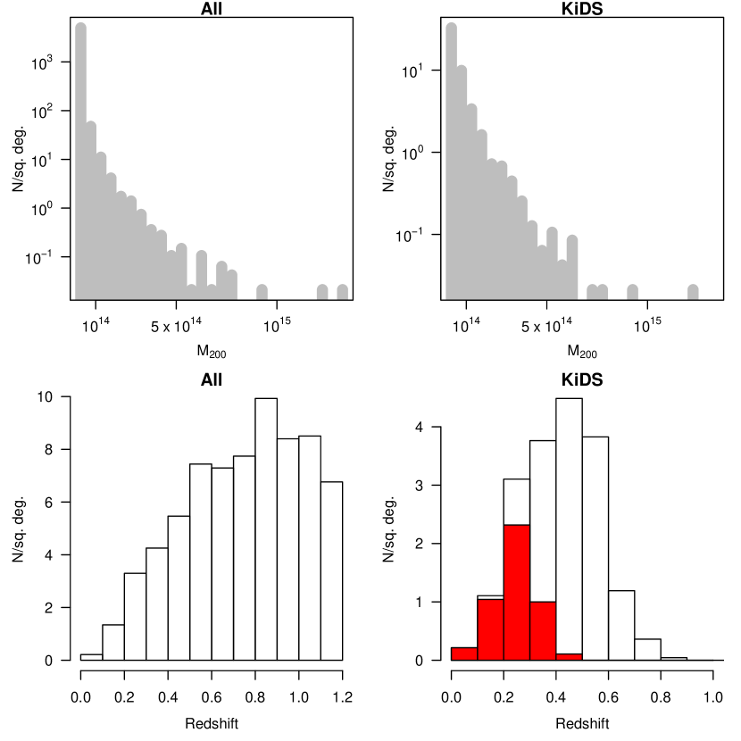
The evolution of the number density of massive galaxy clusters is an important cosmological probe (e.g. Allen et al., 2011), particularly at high redshifts (). It is therefore important to increase the number of known galaxy clusters. The number of clusters as a function of mass and redshift detected in a KiDS–like survey was evaluated using the mock catalogues derived by Henriques et al. (2012, H12 hereafter), which are based on the semi–analytic galaxy models built by Guo et al. (2011) for the Millennium Simulation (MS; Springel et al., 2005). In particular, these mock catalogues provide SDSS photometry for galaxies in 24 light cones, 1.4 1.4 deg2 each, as well as the mass of their parent halos. Galaxy clusters were identified in the mock catalogues following the recipe by Milkeraitis et al. (2010, see their Table 1): cluster members were defined as those with the same friends-of-friends identification number and of their parent halo, and clusters with less than five members were rejected. Next, galaxies with magnitudes brighter than the KiDS limiting magnitudes (see Fig. 9) were selected: we further considered only those clusters with at least 10 galaxies after the latter selection.
Figure 25 shows the mass and redshift distribution of the simulated clusters in H12 before (left) and after (right) the KiDS magnitude cuts were applied: it can be seen that a KiDS–like survey can probe galaxy clusters in the redshift range, extending the cluster detection studies based on SDSS data, which are incomplete beyond (e.g. Rykoff et al., 2014; Rozo et al., 2014). For comparison, in the lower right panel we overplot the redshift distribution obtained adopting the SDSS limiting magnitudes ( mag, mag), showing the improvement expected with KiDS for . At the moment, a cluster detection analysis is on-going (Radovich et al., 2015) using the methods described in Bellagamba et al. (2011), which are based on an optimal filter to find galaxy overdensities from the position, photometry and possibly also photometric redshift of the galaxies in the catalogues. Details and first results will be discussed in a separate paper.
6.5 High-redshift Quasar searches
High redshift quasars are direct probes of the Universe less than 1 Gyr () after the Big Bang. They provide fundamental constraints on the formation and growth of the first supermassive black holes (SMBHs), on early star formation, and on the chemical enrichment of the initially metal-free intergalactic and interstellar medium. The existing ensemble of high-redshift QSOs is dominated by luminous objects with exceptionally high accretion rates (close to Eddington) and very large SMBHs ( M⊙). For several reasons it is needed to probe fainter QSOs, well below the ”tip of the iceberg”. This would allow to test SMBH early growth scenarios, which can predict a more common population of faint QSOs (Costa et al., 2014) with lower accretion rates. Furthermore, it would allow a better study of the symbiosis in growth of SMBHs and their stellar hosts over cosmic time. These are hampered currently by potentially severe selection biases when comparing AGN-selected samples at high redshift to the host selected samples at low redshift (Willot et al., 2005; Lauer et al., 2007).
For these reasons we are building up a homogeneous sample of QSOs at by combining KiDS and VIKING and using the -band drop-out technique. The 9-band through photometry from the combined surveys goes up to 2 mag deeper than SDSS, UKIDSS and the Panoramic Survey Telescope & Rapid Response System 1 (Pan-STARRS1; Bañados et al. 2014). So far we have discovered nine such QSOs, where the first four are published in Venemans et al. (2015). KiDS is also a useful ingredient in the detection of very high redshift () QSOs with VIKING. Adding the -band KiDS data in the photometric selection removes 50% of these -band drop-out candidates (Venemans et al., 2013).
6.6 Strong gravitational lens searches
Strong gravitational lensing provides the most accurate and direct probe of mass in galaxies, groups and clusters of galaxies (Bolton et al., 2006; Tortora et al., 2010b). The deep, subarcsecond seeing KiDS images are particularly suitable for a systematic census of lenses based on the identification of arc-like structures around massive galaxies, galaxy groups and galaxy clusters. The angular size of the Einstein ring can be expressed as function of the velocity dispersion as (Schneider et al., 1992):
| (8) |
where and are the angular diameter distance between the lens and source and to the source, respectively. For a typical FWHM in -band, we can expect to detect lensing arcs of gravitational structures with .
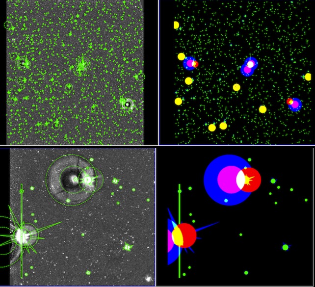
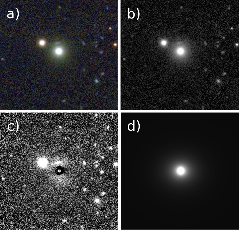
A first search was based on visual inspection. A sample of lens candidates was selected with the following two simple selection criteria, using the photometric redshifts described in Sect. 6.2 and the KiDS-ESO-DR1/2 -band source lists. These criteria are aimed at maximising the lensing probability for the KiDS photometric sensitivities: 1) and 2) . Candidates are visually assessed by inspecting colour images and -band images where the galaxy model obtained with 2DPHOT (see Sect. 6.3) is subtracted. In a control set of 600 candidates in the area overlapping with SDSS, 18 potential lens candidates were identified, half of which have high significance (Napolitano et al., 2015). An example of a good lens candidate is shown in Fig. 26. Another approach consists of automatic selection of lens candidates by filtering the KiDS-ESO-DR1/2 multi-band catalogues for massive early-type galaxies. This is done using colour-colour cuts and automated SED classifiers. In addition, candidates of strongly lensed quasars are identified based on colour and morphology. Candidates from both approaches have been selected further via visual inspection and are being followed up for spectral confirmation.
In the future, as the data volume grows, searches for strong lenses in large-area surveys such as KiDS will have to be performed with (semi-)automated techniques (Alard 2006, More et al. 2012, Gavazzi et al. 2014, Joseph et al. 2014), as the numbers of typical host galaxy candidates can be of the order of thousands per square degree, rendering visual inspection prohibitive. However, current automatic lens-finding tools are not perfect and all automated techniques are still being tested on simulated data (e.g. Metcalf & Petkova 2014, Gavazzi et al. 2014).
7 Summary and outlook
The Kilo-Degree Survey is a 1500 square degree optical imaging survey in four filters () with the VLT Survey Telescope. Together with its near-infrared sister survey VIKING, a nine-band optical-infrared data set will be produced. While KiDS was primarily designed as a tomographic weak gravitational lensing survey, many secondary science cases are pursued.
In this paper the first two data releases (KiDS-ESO-DR1 and KiDS-ESO-DR2) are presented, comprising a total of 148 survey tiles, or 160 square degrees. The data products of these two public data releases were produced using a fine-tuned version of the Astro-WISE optical pipeline (McFarland et al., 2013), complemented with the automated Pulecenella masking software and the KiDS-CAT source extraction software. Data products include calibrated stacked images, weight maps, masks, source lists, and a multi-band source catalogue. Data can be accessed through the ESO Science Archive, the Astro-WISE system, and the KiDS website (see Sect. 2.6 for the relevant links).
The achieved data quality is very close to expectations, with a very small PSF ellipticity over the full FOV and typical limiting magnitudes (5 AB in 2″ aperture) of 24.3, 25.1, 24.9 and 23.8 in , , and , respectively. As the designated lensing band, -band receives the best dark seeing conditions, resulting in an median PSF size of 0.65″, with PSF size variations over the FOV usually 15%. Within survey tiles, the photometry is stable to 2%, but since the photometric calibration is performed using nightly zero-points, photometric offsets between tiles are present due to extinction variations; this will be improved in future data releases. The multi-band source catalogue provided is based on detection in -band and 98% complete to 24.0.
Early weak-lensing applications (Sifón et al., 2015; Viola et al., 2015; van Uitert et al., 2015) of KiDS data rely on the KiDS-ESO-DR1 and -DR2 data products presented here for photometric redshifts, while galaxy shape measurements are based on a dedicated pipeline (see Erben et al., 2013; Miller et al., 2013). Other applications of KiDS-ESO-DR1 and -DR2 data include galaxy structural parameter studies, cluster detection, strong gravitational lens detection, and high-redshift QSO searches. The latter has resulted in the detection of nine QSOs to date (Venemans et al. in prep).
Future data releases, apart from adding more survey tiles to the currently covered area, are foreseen to include additional, value-added data products. During the first years of survey operations the observational data rate has been hampered by several factors, causing slower progress than anticipated. Together with ESO the KiDS team has been working on various improvements, which has led to a significant increase in survey speed since early 2014. At the current rate the survey is expected to be completed by 2019, but continuing efforts to enhance telescope and operational efficiency are expected to lead to further improvements.
Acknowledgements.
Based on data products from observations made with ESO Telescopes at the La Silla Paranal Observatory under programme IDs 177.A-3016, 177.A-3017 and 177.A-3018, and on data products produced by Target/OmegaCEN, INAF-OACN, INAF-OAPD and the KiDS production team, on behalf of the KiDS consortium. The KiDS production team acknowledge support by NWO-M grants. OmegaCEN is financially supported by NOVA and Target. Members of INAF-OAPD and INAF-OACN also acknowledge the support from the Department of Physics & Astronomy of the University of Padova, and of the Department of Physics of Univ. Federico II (Naples). Target is supported by Samenwerkingsverband Noord Nederland, European fund for regional development, Dutch Ministry of economic affairs, Pieken in de Delta, Provinces of Groningen and Drenthe. Target operates under the auspices of Sensor Universe. This work has made use of Astro-WISE, which is an on-going project which started from an EU FP5 RTD programme funded by the EC Action ”Enhancing Access to Research Infrastructures”. JdJ, EMH and NI are supported by NWO grant 614.061.610. MR acknowledges support from the Italian MIUR 2010-2011 through the PRIN ”The dark Universe and the cosmic evolution of baryons: from current surveys to Euclid”. AC and CH acknowledge support from the European Research Council under the EC FP7 grant number 240185. HHi is supported by the DFG Emmy Noether grant Hi 1495/2-1. GL wishes to acknowledge partial support from the Italian MIUR through the PRIN ”Cosmology with Euclid”. MP acknowledges financial support from PRIN-INAF 2014. CT has received funding from the European Union Seventh Framework Programme (FP7/2007-2013) under grant agreement n. 267251 “Astronomy Fellowships in Italy” (AstroFIt). JH is funded by NSERC. BJ acknowledges support by an STFC Ernest Rutherford Fellowship, grant reference ST/J004421/1. HH and MBE acknowledge support from the European Research Council FP7 grant number 279396. LVEK is supported in part through an NWO-VICI career grant (project number 639.043.308). MV is funded by grant 614.001.103 from the Netherlands Organisation for Scientific Research (NWO) and from the European Research Council under FP7 grant number 279396. This work was supported by the Deutsche Forschungsgemeinschaft via the project TR33 ‘The Dark Universe’.References
- Ahn et al. (2012) Ahn, C. P., Alexandroff, R., Allende Prieto, C., et al. 2012, ApJS, 203, 21
- Aihara et al. (2011) Aihara, H., Allende Prieto, C., An, D., et al. 2011, ApJS, 193, 29
- Alard (2006) Alard, C. 2006, ArXiv Astrophysics e-prints, astro-ph/0606757
- Allen et al. (2011) Allen, S. W., Evrard, A. E., Mantz, A. B. 2011, ARA&A, 49, 409
- Arnouts et al. (1999) Arnouts, S., Cristiani, S., Moscardini, L., et al. 1999, MNRAS, 310, 540
- Bañados et al. (2014) Bañados, E., Venemans, B. P., Morganson, E., et al. 2014, AJ, 148, 14
- Begeman et al. (2013) Begeman, K., Belikov, A. N., Boxhoorn, D. R., & Valentijn, E. A. 2013, ExA, 35, 1
- Bellagamba et al. (2011) Bellagamba, F., Maturi, M., Hamana, T. et al. 2011, MNRAS, 413, 1145
- Benítez (2000) Benítez N. 2000, ApJ, 536, 571
- Benjamin et al. (2010) Benjamin, J., van Waerbeke, L., Ménard, B., & Kilbinger, M. 2010, MNRAS, 408, 1168
- Bertin & Arnouts (1996) Bertin, E., & Arnouts, S. 1996, A&AS, 117, 393
- Bertin et al. (2002) Bertin, E., Mellier, Y., Radovich, M., et al. 2002, Astronomical Data Analysis Software and Systems XI, 281, 228
- Bertin (2006) Bertin, E. 2006, ASP Conf. Series 351, 112
- Biviano et al. (2013) Biviano, A., Rosati, P., Balestra, I., et al. 2013, A&A, 558, A1, 22
- Blanton et al. (2005) Blanton, M. R., Lupton, R. H., Schlegel, D. J., et al. 2005, ApJ, 631, 208
- Bolton et al. (2006) Bolton, A. S., Burles, S., Koopmans, L. V. E., Treu, T., & Moustakas, L. A. 2006, ApJ, 638, 703
- Brescia et al. (2013) Brescia, M., Cavuoti, S., D’Abrusco, R., Longo, G., & Mercurio, A. 2013, ApJ, 772, 140
- Brescia et al. (2014) Brescia, M., Cavuoti, S., De Stefano, V., & Longo, G. 2014, submitted to A&A
- Bruzual & Charlot (2003) Bruzual, G., & Charlot, S. 2003, MNRAS, 344, 1000
- Capaccioli et al. (2012) Capaccioli, M., Schipani, P., de Paris, G., et al. 2012, in Science from the Next Generation Imaging and Spectroscopy Surveys, p. 1
- Cavuoti et al. (2012) Cavuoti, S., Brescia, M., Longo, G. & Mercurio, A. 2012, A&A, 546, A13, 1
- Cavuoti et al. (2015) Cavuoti, S., Brescia, M., Tortora, C., et al. 2015, MNRAS, 452, 3100
- Coe et al. (2006) Coe D., Benítez N., Sánchez S. F., et al. 2006, AJ, 132, 926
- Colless et al. (2001) Colless, M. M., Dalton, G., Maddox, S., et al. 2001, MNRAS, 328, 1039
- Costa et al. (2014) Costa, T., Sijacki, D., Trenti, M., & Haehnelt, M. G. 2014, MNRAS, 439, 2146
- Davidon (1991) Davidon, W.C., 1991. SIAM Journal on Optimization, 14, 567
- de Jong et al. (2013) de Jong, J. T. A., Verdoes Kleijn, G. A., Kuijken, K. H., & Valentijn, E. A. 2013, ExA, 35, 25
- De Lucia et al. (2006) De Lucia, G., Springel, V., White, S. D. M., Croton, D., & Kauffmann, G. 2006, MNRAS, 366, 499
- Drew et al. (2014) Drew, J. E., Gonzalez-Solares, E., Greimel, R., et al. 2014, MNRAS, 440, 2036
- Driver et al. (2011) Driver, S. P., Hill, D. T., Kelvin, L. S. et al. 2011, MNRAS, 413, 971
- Edge et al. (2013) Edge, A., Sutherland, W., Kuijken, K., et al. 2013, The Messenger, 154, 32
- Erben et al. (2009) Erben, T., Hildebrandt, H., Lerchster, M., et al. 2009, A&A, 493, 1197
- Erben et al. (2013) Erben T., Hildebrandt, H., Miller, L., et al. 2013, MNRAS, 433, 2545
- Fontanot et al. (2009) Fontanot, F., De Lucia, G., Monaco, P., Somerville, R. S., & Santini, P. 2009, MNRAS, 397, 1776
- Garilli et al. (1999) Garilli, B., Maccagni, D., & Andreon, S. 1999, A&A, 342, 408
- Gavazzi et al. (2014) Gavazzi, R., Marshall, P. J., Treu, T. & Sonnenfeld, A. 2014, ApJ, 785, 144
- Geisser (1975) Geisser, S., 1975, Journal of the American Statistical Association, 70 (350), 320-328
- Guo et al. (2011) Guo, Q., White, S., Boylan-Kolchin, M. et al. 2011, MNRAS, 413, 101
- Henriques et al. (2012) Henriques, B. M. B., White, S. D. M., Lemson, G., et al. 2012, MNRAS, 421, 2904
- Heymans et al. (2012) Heymans, C., van Waerbeke, L., Miller, L., et al. 2012, MNRAS, 427, 146
- Hildebrandt et al. (2012) Hildebrandt H., Erben, T., Kuijken, K., et al. 2012, MNRAS, 421, 2355
- Hilz et al. (2013) Hilz, M., Naab, T., & Ostriker J. P. 2013, MNRAS, 429, 2924
- Hough (1962) Hough, P. V. C. 1962, U.S. Patent 3,069,654
- Ivezić et al. (2004) Ivezić, Ž, Lupton, R. H., Schlegel, D., et al. 2004, AN, 325, 583
- Iwert et al. (2006) Iwert. O., Baade, D., Balestra, A., et al. 2006, Proc. SPIE 6276, 62760A
- Joseph et al. (2014) Joseph, R., Courbin, F., Metcalf, R. B., et al. 2014, A&A, 566, 63
- Kilbinger et al. (2014) Kilbinger, M., Bonnett, C. & Coupon, J. 2014, athena: Tree code for second-order correlation functions, Astrophysics Source Code Library (ascl:1402.026)
- Kuijken (2011) Kuijken, K. H. 2011, The Messenger, 146, 8
- Kuijken et al. (2015) Kuijken, K., Heymans, C., Hildebrandt, H., et al. 2015, MNRAS, submitted, arXiv:1507.00738
- La Barbera et al. (2008) La Barbera, F., de Carvalho, R. R., Kohl-Moreira, J. L., et al. 2008, PASP, 120, L681
- La Barbera & de Carvalho (2009) La Barbera, F. & de Carvalho R. R. 2009, ApJ, 699, L76
- La Barbera et al. (2010) La Barbera, F., de Carvalho, R. R., de La Rosa, I. G., et al. 2010, MNRAS, 408, 1313
- La Barbera et al. (2010) La Barbera, F., de Carvalho, R. R., de La Rosa, I. G., et al. 2010, MNRAS, 408, 1313
- La Barbera et al. (2011) La Barbera, F., Ferreras, I., de Carvalho, R. R., et al. 2011, ApJ, 740, L41
- La Barbera et al. (2012) La Barbera, F., Ferreras, I., de Carvalho, R. R., et al. 2012, MNRAS, 426, 2300
- Landolt (1992) Landolt, A. U. 1992, AJ, 104, 340
- Landy & Szalay (1993) Landy, S. D. & Szalay, A. S. 1993, ApJ, 412, 64
- Lauer et al. (2007) Lauer, T. R., Tremaine, S., Richstone, D., & Faber, S. M. 2007, ApJ, 670, 249
- Liske et al. (2014) Liske, J., Baldry, I. K., Driver, S. P., et al. 2014, submitted
- Maddox et al. (1990) Maddox, S. J., Efstathiou, G., & Sutherland, W. J. 1990, MNRAS, 246, 433
- McFarland et al. (2013) McFarland, J., Verdoes-Kleijn, G., Sikkema, G., et al. 2013, ExA, 35, 79 (MF13)
- Metcalf & Petkova (2014) Metcalf, R. B. & Petkova, M. 2014, MNRAS, 445, 1942
- Milkeraitis et al. (2010) Milkeraitis, M., van Waerbeke, L., Heymans, C. et al. 2014, MNRAS, 406, 673
- Miller et al. (2013) Miller L., Heymans, C., Kitching, T. D., et al. 2013, MNRAS, 429, 2858
- More et al. (2012) More, A., Cabanac, R., More, S., et al. 2012, ApJ, 749, 38
- Napolitano et al. (2015) Napolitano N. R., Covone G., Roy N., et al. 2015, arXiv:1507.00733
- Padmanabhan et al. (2008) Padmanabhan, N., Schlegel, D. J., Finkbeiner, D. P., et al. 2008, ApJ, 674, 2
- Peng et al. (2010) Peng, C. Y., Ho, L. C., Impey, C. D. & Rix, H.-W. 2010, AJ, 139, 2097
- Radovich et al. (2015) Radovich, M., Puddu, E., Bellagamba, F., et al. 2015, Proc. conference ”The Universe of Digital Sky Surveys”, Naples, Italy (Nov. 25-28, 2014), arXiv:1507.00743
- Rozo et al. (2014) Rozo, E., Rykoff, E. S., Bartlett, J. G. & Melin, J. B. 2015, MNRAS, 450, 592
- Rykoff et al. (2014) Rykoff, E. S., Rozo, E., Busha, M. T. et al. 2014, ApJ, 785, 104
- Schlegel et al. (1998) Schlegel, D. J., Finkbeiner, D. P., & Davis, M. 1998, ApJ, 500, 525
- Schneider et al. (1992) Schneider, P., Ehlers, J., & Falco, E. E. 1992, Gravitational Lenses (New York: Springer)
- Shanks et al. (2013) Shanks, T., Belokurov, V., Chehade, B., et al. 2013, The Messenger, 154, 38
- Sifón et al. (2015) Sifón, C., Cacciato, M., Hoekstra, H., et al. 2015, MNRAS, submitted, arXiv:1507.00737
- Shanno (1970) Shanno, D. F., 1970, Math. Comput. 24: 647
- Skrutskie et al. (2006) Skrutskie, M. F., Cutri, R. M. Stiening, R., et al. 2006, AJ, 131, 1163
- Springel et al. (2005) Springel, V., White, S. D. M., Jenkins, A. et al. 2005, Nature, 435, 629
- Tortora et al. (2010a) Tortora, C., Napolitano, N. R., Cardone, V. F., et al. 2010, MNRAS, 407, 144
- Tortora et al. (2010b) Tortora, C., Napolitano, N. R., Romanowsky, A. J., & Jetzer, P. 2010, ApJL, 721, L1
- Tortora et al. (2011a) Tortora, C., Napolitano, N. R., Romanowsky, A. J., et al. 2011a, MNRAS, 418, 1557
- Tortora et al. (2011b) Tortora, C., Romeo, A. D., Napolitano, N. R., et al., 2011b, MNRAS, 411, 627
- Tortora & Napolitano (2012) Tortora, C., & Napolitano, N. R. 2012, MNRAS, 421, 2478
- Tortora et al. (2013) Tortora, C., Pipino, A., D’Ercole, A., Napolitano, N. R., & Matteucci, F. 2013, MNRAS, 435, 786
- Tortora et al. (2014) Tortora, C., Napolitano, N. R., Saglia, R. P., et al. 2014, MNRAS, 445, 162
- Tortora et al. (2015) Tortora, C., La Barbera, F., Napolitano, N. R., et al. 2015, MNRAS, submitted, arXiv:1507.00731
- Trujillo et al. (2006) Trujillo, I., Förster Schreiber, N. M., Rudnick, G., et al. 2006, ApJ, 650, 18
- Trujillo et al. (2007) Trujillo, I., Conselice, C. J., Bundy, K., et al. 2007, MNRAS, 382, 109
- Valentijn et al. (2007) Valentijn, E. A., McFarland, J. P., Snigula, J., et al.: Astro-WISE: chaining to the Universe. 2007, ASPC, 376, 491
- van Uitert et al. (2015) van Uitert, E., et al. (KiDS Collaboration) 2015, ArXiv e-prints
- Venemans et al. (2013) Venemans, B. P., Findlay, J. R., Sutherland, W. J., et al. 2013, ApJ, 779, 24
- Venemans et al. (2015) Venemans, B. P., Verdoes Kleijn, G., Mwebaze, J., et al. 2015, MNRAS, accepted, arXiv:1507.00726
- Verdoes Kleijn et al. (2013) Verdoes Kleijn, G. A., Kuijken, K. H., Valentijn, E. A., et al. 2013, ExA, 35, 103
- Viola et al. (2015) Viola, M., Cacciato, M., Brouwer, M., et al. 2015, MNRAS, accepted, arXiv:1507.00735
- Willot et al. (2005) Willott, C. J., Percival, W. J., McLure, R. J., et al. 2005, ApJ, 626, 657
Appendix A Single-band source list columns
The following table lists the columns that are present in the single-band source lists provided in KiDS-ESO-DR1/2. Note that of the 27 aperture flux columns only the ones for the smallest aperture (2 pixels, or 0.4″ diameter) and the largest aperture (200 pixels, or 40″ diameter) are listed. Note: the label for the aperture of 28.5 pixels is FLUX_APER_28p5.
| Label | Format | Unit | Description |
|---|---|---|---|
| 2DPHOT | J | Source | classification (see section on star/galaxy separation) |
| X_IMAGE | E | pixel | Object position along x |
| Y_IMAGE | E | pixel | Object position along y |
| NUMBER | J | Running object number | |
| CLASS_STAR | E | SExtractor S/G classifier | |
| FLAGS | J | Extraction flags | |
| IMAFLAGS_ISO | J | FLAG-image flags summed over the iso. profile | |
| NIMAFLAG_ISO | J | Number of flagged pixels entering | |
| IMAFLAGS_ISO | J | Number of flagged pixels entering IMAFLAGS_ISO | |
| FLUX_RADIUS | E | pixel | Fraction-of-light radii |
| KRON_RADIUS | E | pixel | Kron apertures in units of A or B |
| FWHM_IMAGE | E | pixel | FWHM assuming a gaussian core |
| ISOAREA_IMAGE | J | pixel2 | Isophotal area above Analysis threshold |
| ELLIPTICITY | E | 1 - B_IMAGE/A_IMAGE | |
| THETA_IMAGE | E | deg | Position angle (CCW/x) |
| MAG_AUTO | E | mag | Kron-like elliptical aperture magnitude |
| MAGERR_AUTO | E | mag | RMS error for AUTO magnitude |
| ALPHA_J2000 | D | deg | Right ascension of barycenter (J2000) |
| DELTA_J2000 | D | deg | Declination of barycenter (J2000) |
| FLUX_APER_2 | E | count | Flux vector within circular aperture of 2 pixels |
| … | … | … | … |
| FLUX_APER_200 | E | count | Flux vector within circular aperture of 200 pixels |
| FLUXERR_APER_2 | E | count | RMS error vector for flux within aperture of 2 pixels |
| … | … | … | … |
| FLUXERR_APER_200 | E | count | RMS error vector for flux within aperture of 200 pixels |
| MAG_ISO | E | mag | Isophotal magnitude |
| MAGERR_ISO | E | mag | RMS error for isophotal magnitude |
| MAG_ISOCOR | E | mag | Corrected isophotal magnitude |
| MAGERR_ISOCOR | E | mag | RMS error for corrected isophotal magnitude |
| MAG_BEST | E | mag | Best of MAG_AUTO and MAG_ISOCOR |
| MAGERR_BEST | E | mag | RMS error for MAG_BEST |
| BACKGROUND | E | count | Background at centroid position |
| THRESHOLD | E | count | Detection threshold above background |
| MU_THRESHOLD | E | arcsec-2 | Detection threshold above background |
| FLUX_MAX | E | count | Peak flux above background |
| MU_MAX | E | arcsec-2 | Peak surface brightness above background |
| ISOAREA_WORLD | E | deg2 | Isophotal area above Analysis threshold |
| XMIN_IMAGE | J | pixel | Minimum x-coordinate among detected pixels |
| YMIN_IMAGE | J | pixel | Minimum y-coordinate among detected pixels |
| XMAX_IMAGE | J | pixel | Maximum x-coordinate among detected pixels |
| YMAX_IMAGE | J | pixel | Maximum y-coordinate among detected pixels |
| X_WORLD | D | deg | Baryleft position along world x axis |
| Y_WORLD | D | deg | Baryleft position along world y axis |
| XWIN_IMAGE | E | pixel | Windowed position estimate along x |
| YWIN_IMAGE | E | pixel | Windowed position estimate along y |
| X2_IMAGE | D | pixel2 | Variance along x |
| Y2_IMAGE | D | pixel2 | Variance along y |
| XY_IMAGE | D | pixel2 | Covariance between x and y |
| X2_WORLD | E | deg2 | Variance along X-WORLD (alpha) |
| Y2_WORLD | E | deg2 | Variance along Y-WORLD (delta) |
| XY_WORLD | E | deg2 | Covariance between X-WORLD and Y-WORLD |
| CXX_IMAGE | E | pixel-2 | Cxx object ellipse parameter |
| CYY_IMAGE | E | pixel-2 | Cyy object ellipse parameter |
| CXY_IMAGE | E | pixel-2 | Cxy object ellipse parameter |
| CXX_WORLD | E | deg-2 | Cxx object ellipse parameter (WORLD units) |
| CYY_WORLD | E | deg-2 | Cyy object ellipse parameter (WORLD units) |
| CXY_WORLD | E | deg-2 | Cxy object ellipse parameter (WORLD units) |
| A_IMAGE | D | pixel | Profile RMS along major axis |
| B_IMAGE | D | pixel | Profile RMS along minor axis |
| A_WORLD | E | deg | Profile RMS along major axis (WORLD units) |
| B_WORLD | E | deg | Profile RMS along minor axis (WORLD units) |
| THETA_WORLD | E | deg | Position angle (CCW/world-x) |
| THETA_J2000 | E | deg | Position angle (east of north) (J2000) |
| ELONGATION | E | deg | A_IMAGE/B_IMAGE |
| ERRX2_IMAGE | E | pixel2 | Variance of position along x |
| ERRY2_IMAGE | E | pixel2 | Variance of position along y |
| ERRXY_IMAGE | E | pixel2 | Covariance of position between x and y |
| ERRX2_WORLD | E | deg2 | Variance of position along X-WORLD (alpha) |
| ERRY2_WORLD | E | deg2 | Variance of position along Y-WORLD (delta) |
| ERRXY_WORLD | E | deg2 | Covariance of position X-WORLD/Y-WORLD |
| ERRCXX_IMAGE | E | pixel-2 | Cxx error ellipse parameter |
| ERRCYY_IMAGE | E | pixel-2 | Cyy error ellipse parameter |
| ERRCXY_IMAGE | E | pixel-2 | Cxy error ellipse parameter |
| ERRCXX_WORLD | E | deg-2 | Cxx error ellipse parameter (WORLD units) |
| ERRCYY_WORLD | E | deg-2 | Cyy error ellipse parameter (WORLD units) |
| ERRCXY_WORLD | E | deg-2 | Cxy error ellipse parameter (WORLD units) |
| ERRA_IMAGE | E | pixel | RMS position error along major axis |
| ERRB_IMAGE | E | pixel | RMS position error along minor axis |
| ERRA_WORLD | E | deg | World RMS position error along major axis |
| ERRB_WORLD | E | deg | World RMS position error along minor axis |
| ERRTHETA_IMAGE | E | deg | Error ellipse position angle (CCW/x) |
| ERRTHETA_WORLD | E | deg | Error ellipse position angle (CCW/world-x) |
| ERRTHETA_J2000 | E | deg | J2000 error ellipse pos. angle (east of north) |
| FWHM_WORLD | E | deg | FWHM assuming a gaussian core |
| ISO0 | J | pixel2 | Isophotal area at level 0 |
| ISO1 | J | pixel2 | Isophotal area at level 1 |
| ISO2 | J | pixel2 | Isophotal area at level 2 |
| ISO3 | J | pixel2 | Isophotal area at level 3 |
| ISO4 | J | pixel2 | Isophotal area at level 4 |
| ISO5 | J | pixel2 | Isophotal area at level 5 |
| ISO6 | J | pixel2 | Isophotal area at level 6 |
| ISO7 | J | pixel2 | Isophotal area at level 7 |
| SLID | K | Source list ID | |
| SID | K | Source ID within the source list | |
| HTM | K | Hierarchical Triangular Mesh (level 25) | |
| FLAG | K | Not used |
Appendix B Multi-band catalogue
The following table lists the columns that are present in the multi-band catalog provided in KiDS-ESO-DR2.
| Label | Format | Unit | Description |
| Measurements based on -band detection image | |||
| ID | 23A | Source identifier | |
| RAJ2000 | D | deg | Right ascension (J2000) |
| DECJ2000 | D | deg | Declination (J2000) |
| SG2DPHOT | K | Source classification | |
| A | D | pixel | Linear semi major axis |
| B | D | pixel | Linear semi minor axis |
| CLASS_STAR | E | SExtractor star/galaxy classifier | |
| KRON_RADIUS | E | pixel | Kron-radius used for MAG_AUTO |
| POSANG | E | deg | Position angle |
| SEQNR | K | -band sequence number | |
| Measurements provided for each filter | |||
| FLUXERR_APER_100_¡filter¿ | E | count | flux error in 100 pixel aperture |
| FLUXERR_APER_10_¡filter¿ | E | count | flux error in 10 pixel aperture |
| FLUXERR_APER_14_¡filter¿ | E | count | flux error in 14 pixel aperture |
| FLUXERR_APER_25_¡filter¿ | E | count | flux error in 25 pixel aperture |
| FLUXERR_APER_40_¡filter¿ | E | count | flux error in 40 pixel aperture |
| FLUXERR_APER_4_¡filter¿ | E | count | flux error in 4 pixel aperture |
| FLUXERR_APER_6_¡filter¿ | E | count | flux error in 6 pixel aperture |
| FLUXERR_APERCOR_100_¡filter¿ | E | count | corrected flux error in 100 pixel aperture |
| FLUXERR_APERCOR_10_¡filter¿ | E | count | corrected flux error in 10 pixel aperture |
| FLUXERR_APERCOR_14_¡filter¿ | E | count | corrected flux error in 14 pixel aperture |
| FLUXERR_APERCOR_25_¡filter¿ | E | count | corrected flux error in 25 pixel aperture |
| FLUXERR_APERCOR_40_¡filter¿ | E | count | corrected flux error in 40 pixel aperture |
| FLUXERR_APERCOR_4_¡filter¿ | E | count | corrected flux error in 4 pixel aperture |
| FLUXERR_APERCOR_6_¡filter¿ | E | count | corrected flux error in 6 pixel aperture |
| FLUX_APER_100_¡filter¿ | E | count | flux in 100 pixel aperture |
| FLUX_APER_10_¡filter¿ | E | count | flux in 10 pixel aperture |
| FLUX_APER_14_¡filter¿ | E | count | flux in 14 pixel aperture |
| FLUX_APER_25_¡filter¿ | E | count | flux in 25 pixel aperture |
| FLUX_APER_40_¡filter¿ | E | count | flux in 40 pixel aperture |
| FLUX_APER_4_¡filter¿ | E | count | flux in 4 pixel aperture |
| FLUX_APER_6_¡filter¿ | E | count | flux in 6 pixel aperture |
| FLUX_APERCOR_100_¡filter¿ | E | count | corrected flux in 100 pixel aperture |
| FLUX_APERCOR_10_¡filter¿ | E | count | corrected flux in 10 pixel aperture |
| FLUX_APERCOR_14_¡filter¿ | E | count | corrected flux in 14 pixel aperture |
| FLUX_APERCOR_25_¡filter¿ | E | count | corrected flux in 25 pixel aperture |
| FLUX_APERCOR_40_¡filter¿ | E | count | corrected flux in 40 pixel aperture |
| FLUX_APERCOR_4_¡filter¿ | E | count | corrected flux in 4 pixel aperture |
| FLUX_APERCOR_6_¡filter¿ | E | count | corrected flux in 6 pixel aperture |
| FLUX_RADIUS_¡filter¿ | E | pixel | SExtractor FLUX_RADIUS |
| FWHM_IMAGE_¡filter¿ | E | pixel | SExtractor FWHM_IMAGE |
| FLAG_¡filter¿ | J | SExtractor extraction flag | |
| IMAFLAGS_ISO_¡filter¿ | J | Mask flag | |
| MAGERR_AUTO_¡filter¿ | E | mag | RMS error for MAG_AUTO |
| MAGERR_ISO_¡filter¿ | E | mag | RMS error for MAG_ISO |
| MAG_AUTO_¡filter¿ | E | mag | Kron-like elliptical aperture magnitude |
| MAG_ISO_¡filter¿ | E | mag | Isophotal magnitude |
| NIMAFLAGS_ISO_¡filter¿ | J | Number of masked pixels entering IMAFLAGS_ISO | |
| ISOAREA_IMAGE_¡filter¿ | J | pixel2 | Isophotal aperture |
| XPOS_¡filter¿ | E | pixel | X pixel position ¡filter¿ coadd |
| YPOS_¡filter¿ | E | pixel | Y pixel position ¡filter¿ coadd |