Frozen and almost frozen structures in the compressible rotating fluid

Abstract.

We study a possibility of existence of localized two-dimensional structures, both smooth and non-smooth, that can move without significant change of their shape in a leading stream of compressible barotropic fluid on a rotating plane.

1. Bidimensional model of compressible fluid

We consider the system of barotropic gas dynamics in 2D on the rotating plane,

$$\varrho(\partial_{t}{\bf U}+({\bf U}\cdot\nabla){\bf U}+{\mathcal{L}}{\bf U})+\nabla P(\rho)=0,\quad P=C\rho^{\gamma},\quad C>0,$$ (1)

$$\partial_{t}\varrho+{\rm div}(\varrho{\bf U})=0,$$ (2)

for density $\varrho,$ vector of velocity ${\bf U}$ and pressure $P$, $t\geq 0$, $x\in{\mathbb{R}}^{2}$. Here $\mathcal{L}=lL$, $\,L=\left(\begin{array}[]{cr}0&-1\\ 1&0\end{array}\right)$, $l$ is the Coriolis parameter assumed to be a positive constant, $\gamma\in(1,2)$ is the adiabatic exponent.

Under suitable boundary conditions system (1), (2) implies conservation of mass, momentum and total energy.

Many models of ocean, atmosphere and plasma are approximately two dimensional. In particular, in [1] a procedure of averaging over the hight in a three-dimensional model of atmosphere consisting of compressible rotating polytropic gas was proposed (see also [2]).

Let us introduce a new variable $\pi=P^{\frac{\gamma-1}{\gamma}}.$ For $\pi(t,x)$ and ${\bf U}(t,x)$ we obtain the following system:

$$\partial_{t}{\bf U}+({\bf U}\cdot\nabla){\bf U}+lL{\bf U}+c_{0}\,\nabla\pi=0,\quad\partial_{t}\pi+(\nabla\pi\cdot{\bf U})+(\gamma-1)\pi\,{\rm div}{\bf U}=0,$$

with $c_{0}=\frac{\gamma}{\gamma-1}C^{\frac{1}{\gamma}}.$ Then we change the coordinate system in such a way that the origin of the new system ${\bf x}=(x_{1},x_{2})$ is located at a point ${\bf X}(t)=(X_{1}(t),X_{2}(t))$ (here and below we use the lowercase letters for $\bf x$ to denote the local coordinate system). Now ${\bf U}={\bf u}+{\bf V},$ where ${\bf V}(t)=(V_{1}(t),V_{2}(t))=(\dot{X}_{1}(t),\dot{X}_{2}(t))$. Thus, we obtain a new system

$$\partial_{t}{\bf u}+({\bf u}\cdot\nabla){\bf u}+\dot{\bf V}+l\,L\,({\bf u}+{\bf V})+c_{0}\,\nabla\pi=0,$$ (3)

$$\quad\partial_{t}\pi+(\nabla\pi\cdot{\bf u})+(\gamma-1)\,\pi\,{\rm div}\,{\bf u}\,=\,0.$$ (4)

Given a vector ${\bf V}$, the trajectory can be found by integration from the system $\dot{X}_{i}(t)=V_{i}(t),\,i=1,2.$

In our previous papers [3], [4] we used this approach to find a position of atmospherical vortex, associated with a tropical cyclone.

2. Local and bearing fields separation

We assume that the pressure field $\pi(t,x_{1},x_{2})$ can be separated into two part as $\pi=\pi_{0}+\pi_{1}$, where $\pi_{1}$ is somewhat stronger, however more uniform than $\pi_{0}$. We call $\pi_{0}$ the local field and $\pi_{1}$ the bearing field.

Then we obtain from (3), (4)

$$\left[\partial_{t}{\bf u}+({\bf u}\cdot\nabla){\bf u}+{\mathcal{L}}{\bf u}+c_{0}\,\nabla\pi_{0}\right]+\left[\dot{\bf V}+{\mathcal{L}}\,{\bf V}+c_{0}\,\nabla\pi_{1}\right]=0,\quad\qquad\phantom{\pi_{1}\,{\rm div}\,{\bf u}\,)=\,0}$$

$$\left[\partial_{t}\pi_{0}+(\nabla\pi_{0}\cdot{\bf u})+(\gamma-1)\,\pi_{0}\,{\rm div}\,{\bf u}\right]\,+\,\left[\partial_{t}\pi_{1}+(\nabla\pi_{1}\cdot{\bf u})+(\gamma-1)\,\pi_{1}\,{\rm div}\,{\bf u}\,\right]=\,0.$$

If we assume that we can find the couple $({\bf u},\pi_{0})$ from the system

$$\partial_{t}{\bf u}+({\bf u}\cdot\nabla){\bf u}+{\mathcal{L}}\,{\bf u}+c_{0}\,\nabla\pi_{0}=Q(t,x),$$ (5)

$$\partial_{t}\pi_{0}+(\nabla\pi_{0}\cdot{\bf u})+(\gamma-1)\,\pi_{0}\,{\rm div}\,{\bf u}=\,0,$$ (6)

with a certain function $Q(t,x)$, then we get a linear equation for $\pi_{1}$,

$$\partial_{t}\pi_{1}+(\nabla\pi_{1}\cdot{\bf u})+\pi_{1}{\rm div}{\bf u}=0,$$ (7)

which can be solved for any initial condition $\pi_{1}(0,{\bf x})$. Further, (5) and (3) imply

$$\dot{\bf V}(t)+{\mathcal{L}}{\bf V}(t)+c_{0}\nabla\pi_{1}(t,{\bf x})=-Q(t,x).$$

Now we set

$$Q=-c_{0}\left[\nabla\pi_{1}(t,{\bf x})-\nabla\pi_{1}(t,{\bf 0})\right].$$ (8)

Thus, we associate the couple $({\bf u},\pi_{0})$ with the local field and the couple $({\bf V},\pi_{1})$ with the bearing field. As we can see, the couple $({\bf u},\pi_{0})$ is independent of the bearing field ”up to the function $Q$.” If the solution $({\bf u},\pi_{0})$ to system (5), (6) is found, we can find $({\bf V},\pi_{1})$ from linear equations.

If $Q=0$, then the bearing field does not influence on the local field and in this sense we will talk on a complete separation of he bearing and local fields. Evidently, this will be only if $\pi_{1}$ is linear with respect to the space variables. If $|Q|<\delta$ for sufficiently small $\delta>0$, we can talk about a ”$\delta$- approximate” separation of fields, $Q$ plays a role of discrepancy. This discrepancy is a measure of separability of the local and bearing fields.

The position of the center of the moving coordinate system can be found from the following equation:

$$\ddot{\bf X}(t)+{\mathcal{L}}\dot{\bf X}(t)+c_{0}\nabla\pi_{1}(t,{\bf x})\Big{|}_{{\bf x}=0}=0.$$ (9)

As follows from the computer modeling made in [4], even for real meteorological data the position of center of tropical cyclone found by means of equation (9) is quite accurate.

3. Steady nonhomogeneous incompressible flow

We look for a solution of the local field with special properties, namely, a steady divergence free solution. If the discrepancy $Q=0$, then this solution can be considered as a ”frozen pattern” into a leading stream. If the discrepancy is small, we can talk only on an ”almost frozen pattern”, since the right-hand side in equation (5), that depends on the properties of the bearing field, influences the solution.

Thus, let us assume that

$${\bf u}\mbox{\quad does not depend of}\quad t,\quad{\bf u}(0)=0\mbox{\quad and \quad}{\rm div\,\bf u}=0.$$

This means that there exists a stream function $\Phi(x_{1},x_{2})$ such that

$${\bf u}=\nabla_{\bot}\Phi=(\Phi_{x_{2}},-\Phi_{x_{1}}).$$

Equations (6) and (5) result

$$(\nabla\pi_{0}\cdot\nabla_{\bot}\Phi)=0,$$ (10)

$$(\nabla_{\bot}\Phi\cdot\nabla)\nabla_{\bot}\Phi+lL\nabla_{\bot}\Phi+c_{0}\nabla\pi_{0}=0.$$ (11)

We take the inner product of (11) and $\nabla_{\bot}\Phi$ and get

$$\Phi_{x_{1}x_{2}}\,((\Phi_{x_{2}})^{2}-(\Phi_{x_{1}})^{2}))=\,\Phi_{x_{1}}\,\Phi_{x_{2}}\,(\Phi_{x_{2}x_{2}}-\Phi_{x_{1}x_{1}}).$$ (12)

The solution of (12) have to satisfy the identity

$$\nabla\times((\nabla_{\bot}\Phi\cdot\nabla)\nabla_{\bot}\Phi)=0.$$ (13)

Equations (12) and (13) are equivalent to

$$J(\Phi,|\nabla\Phi|^{2})=0,$$ (14)

and

$$J(\Phi,\Delta\Phi)=0,$$ (15)

respectively, where $J$ is the Jacobian. The stream function $\Phi$ has to satisfy both (14) and (15), and for smooth $\Phi$ the function $\pi_{0}$ can be restored up to a constant as

$$\pi_{0}\,=\,-\,\frac{1}{c_{0}}\,\left[\int(\Phi_{x_{2}}\Phi_{x_{1}x_{2}}-\Phi_{x_{1}}\Phi_{x_{2}x_{2}}+l\Phi_{x_{1}})\,dx_{1}+\right.$$

$$\left.\int(-\Phi_{x_{2}}\Phi_{x_{1}x_{1}}+\Phi_{x_{1}}\Phi_{x_{1}x_{2}}+l\Phi_{x_{2}})\,dx_{2}\right]=$$

$$-\frac{1}{c_{0}}\,l\Phi+\left[\int(\Phi_{x_{2}}\Phi_{x_{1}x_{2}}-\Phi_{x_{1}}\Phi_{x_{2}x_{2}})\,dx_{1}+\int(-\Phi_{x_{2}}\Phi_{x_{1}x_{1}}+\Phi_{x_{1}}\Phi_{x_{1}x_{2}})\,dx_{2}\right].$$ (16)

There are two evident classes of solution to (14) and (15):

$$\Phi=\bar{\Phi}(x_{1}^{2}+x_{2}^{2})$$

and

$$\Phi=\bar{\Phi}(x_{i}),\,i=1,2,$$

with arbitrary smooth function of one variable $\bar{\Phi}$. In particular, $\bar{\Phi}$ can be compactly supported.

The first case corresponds to a steady vortex. In the meteorological model this pattern can be associated with a tropical cyclone in the mature stage of development.

The second case corresponds to a shear flow and can be associated with an atmospheric front.

Remark 3.1.

If $\pi_{0}=\rm const$, then the condition (10) is eliminated and the problem can be reduced to the solution of the Euler equations. Even in this case possible steady solutions can be very complicate [5], [6], [7].

Remark 3.2.

Equations (14) and (15) imply the Dubreil-Jacotin equation [8]

$$\Delta\Phi+\frac{\pi_{0}^{\prime}(\Phi)}{2(\gamma-1)\pi_{0}(\Phi)}|\nabla\Phi|^{2}=F(\Phi)$$

if we take into account that $\pi_{0}=\pi_{0}(\Phi)$. The last property follows from (10). The arbitrary functions $\pi_{0}(\Phi)$ and $F(\Phi)$ give initial distribution of density and vorticity.

3.1. Algorithm of solution, the smooth case

Theorem 3.1.

Let $\Phi(x_{1},x_{2})$ be a smooth solution to the system

$$|\nabla\Phi|^{2}=G(\Phi),$$ (17)

$$\Delta\Phi=R(\Phi),$$ (18)

with a differentiable function $G$ and integrable function $R$. Then $\Phi$ solves (14),(15), and therefore it is a part of solution to the system (10), (11).

Proof.

Equations (17) and (18) means that $|\nabla\Phi|^{2}$ and $\Phi$, $\Delta\Phi$ and $\Phi$, respectively, are functionally dependent, this results (14) and (15). Thus, $\Phi$ solves the system (10), (11) together with $\pi_{0}$ found by (16). Namely, taking into account (17) and (18) we obtain

$$\pi_{0}\,=-\,\frac{1}{2c_{0}}\,\left[\int(|\nabla\Phi|^{2}\,-\,2R_{1}(\Phi)+2l\Phi)_{x_{1}}\,dx_{1}+\right.$$

$$\left.\int(|\nabla\Phi|^{2}\,-\,2R_{1}(\Phi)+2l\Phi)_{x_{2}}\,dx_{2}\right]=$$

$$\frac{1}{2c_{0}}\,\left(|\nabla\Phi|^{2}-2R_{1}(\Phi)-2l\Phi\right)\,+\,\rm const,$$

where $R_{1}=\int\limits_{\Phi_{0}}^{\Phi}R(\eta)d\eta.$

∎

3.2. Relation with the eikonal equation

Proposition 3.1.

Assume that a function $\xi$ satisfies in a domain $\Omega$ the standard eikonal equation

$$|\nabla\xi|^{2}=1.$$ (19)

Then any differentiable monotone function $\Phi=\mathcal{F}(\xi)$ satisfies equation (17) with $G(\Phi)=(\Phi^{\prime}(\xi))^{2},$ $\xi=\mathcal{F}^{-1}(\Phi)$.

Proof.

Proof is a direct computation. ∎

4. Construction of localized frozen patterns

4.1. The smooth case

Let $\Omega$ be a compact domain in ${\mathbb{R}}^{2}$ with smooth boundary. We assume that there exist a couple of functions $G(\Phi),R(\Phi))$ such that the stream function $\Phi$ satisfies equations (17), (18) for $x\in\Omega$ in the classical sense and

$$\Phi|_{\partial\Omega}\,=\,0,\quad\nabla\Phi|_{\partial\Omega}\,=\,0.$$ (20)

Proposition 4.1.

Let $\Phi\in C^{2}(\overline{\Omega})$ be a solution to (17), (18) for $x\in\Omega$ with boundary conditions (20). Then the solution to (7) in the domain ${\mathbb{R}}^{2}\setminus\Omega$ in the local coordinate system do not depend of the local field.

Proof.

Condition (20) means ${\bf u}|_{\partial\Omega}=0$, therefore the velocity field can be extended smoothly to the whole plane ${\mathbb{R}}^{2}$ as zero. Then the solution to (7) keeps its initial value for $x\notin\Omega$. $\square$ ∎

Thus, the solution to problems (17), (18), (20) gives a ”frozen pattern” inside the domain $\Omega$.

Let us show that the class of solutions satisfying the conditions of Proposition 4.1 is not empty. The simplest situation is where $\Omega$ is a disc of radius $r$. The solution to (21) with boundary value $\phi=r$ is $\xi=\sqrt{x_{1}^{2}+x_{2}^{2}}$, the differentiability fails only at the origin. Nevertheless, the solution to (20) based on (21) can be smooth everywhere in $\Omega$ if we take $F(\xi)=\xi^{2}.$ Further, we can take $F=\lambda(s)$, $s=|\xi^{2}|$, with any smooth monotone on $[0,1]$ function $\lambda$ such that $\lambda(r^{2})=0,$ $\frac{d^{i}\lambda}{ds^{i}}\Big{|}_{s=r^{2}}=\frac{d^{i}\lambda}{ds^{i}}\Big{|}_{s=0}=0,$ $i=1,2$. Further, $\Delta\Phi(\xi)=\Phi^{\prime\prime}(\xi)|\nabla\xi|^{2}+\Phi^{\prime}(\xi)\Delta\xi=\Phi^{\prime\prime}(\xi)+\frac{\Phi^{\prime}(\xi)}{\xi}\equiv R(\xi).$

This example gives a variety of axisymmetric vortex structures.

Remark 4.1.

As follows from [9], Sec.2.3.3, these structures are nonlinearly stable with respect to smooth perturbations keeping zero boundary conditions.

4.2. Non-smooth case

Now we consider non-classical solution to the system (17), (18), allowing to construct the ”frozen patterns” containing discontinuities.

4.2.1. Generalized solution to the eikonal equation (17)

It is well known that the problem of constructing a nonlocal theory of the Cauchy problem for nonlinear Hamilton-Jacobi equation (in particular, for (19) and (17)) inevitably leads to the necessity of introducing a generalized solution. A natural extension of the notion of the solution in the sense of ”almost everywhere”, i.e. a locally Lipschitz continuous function satisfying the equation everywhere in the considered domain except possibly at the points of a set of zero measure. Generally speaking, this solution is not unique. In [10] it was introduced the following notion of generalized solution, which we formulate applying to our case.

Let $B_{r}(y)=\{x\in{\mathbb{R}}^{2}:|x-y|<r\}$. We denote by ${\mathcal{L}ip}_{loc}(D)$ the totality of functions $f(x)$ defined on a set $D\in{\mathbb{R}}^{2}$ and satisfying the Lipschitz condition on the subset $B_{r}(y)\cap D$. It is known [11] that $f(x)$ has at almost every interior point of $D$ a differential and hence a gradient $\nabla u$.

Further, let $\Omega$ is a bounded domain in ${\mathbb{R}}^{2}$ and $f\in{\mathcal{L}ip}_{loc}(\bar{\Omega})$. We say that $f(x)$ belongs to the stability class $E(\Omega)$ if the following inequality is satisfied for every $x,x+\Delta x,x-\Delta x\in B_{\delta}(y)\subset B_{2\delta}\subset\Omega$, $(\Delta x\neq 0)$:

$$\frac{\Delta^{2}f}{|\Delta x|^{2}}\equiv\frac{f(x+\Delta x)-2f(x)+f(x-\Delta x)}{|\Delta x|^{2}}\geq-C(y,\delta)=\rm const.$$

Definition 4.1.

A function $\Phi\in{\mathcal{L}ip}_{loc}(\bar{\Omega})\cap E(\Omega)$ is called a generalized solution of the Cauchy-Dirichlet problem

$$|\nabla\Phi|^{2}=G(\Phi),\quad\xi|_{\partial\Omega}\,=\,\phi,$$ (21)

where $G(\Phi)$ is a smooth and almost everywhere positive function, if it satisfies equation (17) almost everywhere in $\Omega$ and takes the boundary values.

4.2.2. Generalized solution to the nonlinear Poisson equation (18)

We give the definition of the generalized solution following [12].

Definition 4.2.

$\Phi\in H^{1}(\Omega)$ is called the generalized solution to the boundary problem

$$\Delta\Phi=R(\Phi),\quad x\in\Omega,\quad\Phi=\phi,\quad x\in\partial\Omega,$$

with $R\in L_{2}(\Omega)$, $\phi\in H^{1}(\Omega),$ if

$$\Phi-\phi\in{H}_{0}^{1}(\Omega)$$

and

$$\int\limits_{\Omega}(\nabla\Phi,\nabla v)\,dx\,=\,-\int\limits_{\Omega}R(\Phi)v\,dx$$

for all $v\in{H}_{0}^{1}(\Omega).$

4.3. Example of discontinuous frozen pattern

Now we construct a discontinuous solution to the system (17), (18) in the sense of Definitions 4.1 and 4.2, satisfying zero boundary conditions.

We consider the domain $\Omega$ such that $(x_{1},x_{2})\in\Omega$ if $x_{1}^{2}+x_{2}^{2}<1$ and $x_{1}<\frac{1}{2}$.

It can be readily checked that the function

$$\xi(x_{1},x_{2})=\left\{\begin{array}[]{cc}2x_{1},&-\sqrt{3}x_{1}<x_{2}<\sqrt{3}x_{1},\\ \sqrt{x_{1}^{2}+x_{2}^{2}},&otherwise,\end{array}\right.$$

solves the eikonal equation (19) in $\Omega$ with boundary value $\xi=1$. Let us take again as $F=\lambda(s)$, $s=|\xi^{2}|$, any monotone smooth function on $[0,1]$ such that $\lambda(1)=0,$ $\frac{d^{i}\lambda}{ds^{i}}\Big{|}_{s=r^{2}}=\frac{d^{i}\lambda}{ds^{i}}\Big{|}_{s=0}=0,$ $i=1,2$.

Thus, $\Phi\in{\mathcal{L}ip}_{loc}(\bar{\Omega})$ solves (17) and (18) in the sense of Definition 4.2 with $R(\Phi)=\Phi^{\prime\prime}(\xi)+\frac{\Phi^{\prime}(\xi)}{\xi}(1-\chi(\Omega_{1})),$ where $\chi(\Omega_{1})$ is the characteristic function of the set $\Omega_{1}$, where $\Omega_{1}$ is a subset of $\Omega$, consisting of points $(x_{1},x_{2})$ such that $-\sqrt{3}x_{1}<x_{2}<\sqrt{3}x_{1}$. Moreover, $\Phi$ satisfies the boundary conditions (20). Fig.1 presents the velocity field for this case. The function $\lambda$ was chosen such that the pressure $\pi_{0}$ in the center is lower that on the boundary of $\Omega$, therefore the vorticity is cyclonic (anticlockwise). A couple of lines of discontinuities inside the vortical structure can be used for modeling of cold and warm fronts in a cyclone.

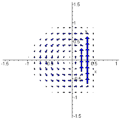
Figure 1.

5. Estimate of the discrepancy

5.1. Smooth case

Proposition 5.1.

Let the stream function $\Phi$, the solution to (17) and (18), be differentiable in ${\mathbb{R}}^{2}$. Then the discrepancy $Q$ (see (8)) is completely defined by initial data for the bearing field $\pi_{1}$.

Proof.

Since $|Q|^{2}\leq 4c_{0}^{2}\sup\limits_{{\bf x}\in{\mathbb{R}}^{2}}|\nabla\pi_{1}(t,{\bf x})|^{2}$, it is enough to prove that

$$\sup\limits_{{{\bf x}\in\mathbb{R}}^{2}}|\nabla\pi_{1}(t,{\bf x})|^{2}\leq\sup\limits_{{{\bf x}\in\mathbb{R}}^{2}}|\nabla\pi_{1}(0,{\bf x})|^{2}.$$ (22)

Due to the divergence-free condition equation (7) has the form

$$\partial_{t}\pi_{1}+(\nabla\pi_{1}\cdot{\bf u})=0.$$

We take the gradient of this equation and then multiply by $\nabla\pi_{1}$ to obtain the transport equation with smooth coefficients $(u_{1},u_{2})$

$$\partial_{t}|\nabla\pi_{1}|^{2}+(\nabla|\nabla\pi_{1}|^{2}\cdot{\bf u})=0.$$ (23)

Thus, the initial value are transported along smooth characteristic curves. This immediately implies (22). ∎

5.2. Non-smooth case

Many papers are devoted to the transport equation with non-smooth coefficients. R.J. DiPerna and P.-L. Lions have proved this uniqueness result under the assumption the coefficients are in the Sobolev class $W^{1,1}$ (locally in space), and later L. Ambrosio extended this result to coefficients of class $BV$ (locally in space). Previous results on two-dimensional transport equation are due to Bouchut and Desvillettes [13], Hauray [14], Colombini and Lerner [15].

To show the maximum principle for (23) in the case on non-smooth velocity ${\bf u}$, we use the following theorem on the well-posedness of the transport equation proved in [16], [17]:

Theorem 5.1.

([16]) Let ${\bf b}:{\mathbb{R}}^{2}\to{\mathbb{R}}^{2}$ be a bounded, divergence-free, autonomous vector field on the plane admitting a Lipschitz compactly supported potential $f:{\mathbb{R}}^{2}\to{\mathbb{R}}$, that is $\bf b=\nabla_{\bot}f$. The Cauchy problem for

$$u_{t}+{\rm div}({\bf b}u)=0$$

admits a unique bounded generalized solution in the sense of distributions for every bounded initial datum if and only if the potential $f$ satisfies the weak Sard property.

Corollary 5.1.

Let the stream-function $\Phi$, taking part of the generalized solution to system (10), (11) be Lipschitz, compactly supported and $|\nabla\Phi|\neq 0$ almost everywhere. Then

$$\|\nabla\pi_{1}(t,{\bf x})\|_{L^{\infty}}\leq\|\nabla\pi_{1}(0,{\bf x})\|_{L^{\infty}},$$

therefore the discrepancy is completely defined by initial data for $\pi_{1}$.

Proof.

Ii is enough to write (23) in the divergent form

$$\partial_{t}|\nabla\pi_{1}|^{2}+{\rm div}(|\nabla\pi_{1}|^{2}\nabla_{\bot}\Phi)=0.$$

and apply Theorem 5.1. As noticed in [16], the weak Sard property is implied by $|\nabla\Phi|\neq 0$ almost everywhere. ∎

References

- [1] Obukhov, A.M. On the geostrophical wind Izv.Acad.Nauk (Izvestiya of Academy of Science of URSS), Ser. Geography and Geophysics, XIII(1949), 281–306.
- [2] Pedlosky, J. Geophysical fluid dynamics, Springer-Verlag, New York, 1979.
- [3] O.S. Rozanova, J-L. Yu, C-K. Hu, Typhoon eye trajectory based on a mathematical model: Comparing with observational data. Nonlinear Analysis: Real World Applications, 11(2010), 1847–1861.
- [4] O.S. Rozanova, J-L. Yu, C-K. Hu. On the position of vortex in a two-dimensional model of atmosphere, Nonlinear Analysis: Real World Applications, 13(2012), 1941–1954.
- [5] H. M. Wu, E. A. Overman, N. J. Zabusky. Steady-state solutions of the Euler equations in two dimensions: Rotating and translating V-states with limiting cases. I. Numerical algorithms and results, J. Comput. Phys., 53 (1984), 42–71.
- [6] J.Yang, T.Kubota. The steady motion of a symmetric, finite core size, counterrotating vortex pair, SIAM J.Appl.Math. 54(1994) 14–25.
- [7] M.Jia, Y.Gao, F.Huang, S.-Y. Lou, J.-L Sun, X.-Y. Tang. Vortices and vortex sources of multiple vortex interaction systems, Nonlinear Analysis: Real World Applications, 13(2012) 2079–2095.
- [8] Dubreil-Jacotin M. L. Sur les théorèmes d’existence relatifs aux ondes permanentes periodiques à deux dimensions dans les liquides hétŕogènes. J. Math. Pures Appl, 13(1937), 217 – 291.
- [9] Padula M. Asymptotic Stability of Steady Compressible Fluids. Lecture Notes In Mathematics. Springer: Berlin, Heidelberg, 2011.
- [10] S.N.Kruzhkov. Generalized solution of the Hamilton-Jacobi equations of eikonal tipe. I. Formulation of the problems; existence, uniqueness and stability theorems; some properties of solutions, Math. URSS Sbornik 23 (1975), 406-446.
- [11] L.C. Evans, R.F. Gariepy. Measure theory and fine properties of functions. Studies in Advanced Mathematics. CRC Press, Boca Raton, FL, 1992.
- [12] L.C. Evans, Partial Differential Equations. Second Edition, Graduate Studies in Mathematics. American Mathematical Society, 2010.
- [13] F. Bouchut, L. Desvillettes. On two-dimensional Hamiltonian transport equations with continuous coefficients. Differential Integral Equations 14 (2001), 1015-1024.
- [14] M. Hauray. On two-dimensional Hamiltonian transport equations with coeficients, Ann. Inst. H. Poincare Anal. Non Lineaire 20 (2003), 625–644.
- [15] F.Colombini, N. Lerner. Uniqueness of L1 solutions for a class of conormal vector fields. Contemp. Math. 368 (2005), 133–156.
- [16] G. Alberti, S. Bianchini, G. Crippa. Two-dimensional transport equation with Hamiltonian vector felds, Hyperbolic problems: theory, numerics and applications, pp. 337–346. Proceedings of Symposia in Applied Mathematics, Volume 67, Part 2. American Mathematical Society, Providence, 2009.
- [17] G. Alberti, S. Bianchini, G. Crippa. A uniqueness result for the continuity equation in two dimensions, Journal of the European Mathematical Society, 16(2014), 201–234.