Improving the numerical stability of
fast matrix multiplication

Abstract

Fast algorithms for matrix multiplication, namely those that perform asymptotically fewer scalar operations than the classical algorithm, have been considered primarily of theoretical interest. Apart from Strassen’s original algorithm, few fast algorithms have been efficiently implemented or used in practical applications. However, there exist many practical alternatives to Strassen’s algorithm with varying performance and numerical properties. Fast algorithms are known to be numerically stable, but because their error bounds are slightly weaker than the classical algorithm, they are not used even in cases where they provide a performance benefit.

We argue in this paper that the numerical sacrifice of fast algorithms, particularly for the typical use cases of practical algorithms, is not prohibitive, and we explore ways to improve the accuracy both theoretically and empirically. The numerical accuracy of fast matrix multiplication depends on properties of the algorithm and of the input matrices, and we consider both contributions independently. We generalize and tighten previous error analyses of fast algorithms and compare their properties. We discuss algorithmic techniques for improving the error guarantees from two perspectives: manipulating the algorithms, and reducing input anomalies by various forms of diagonal scaling. Finally, we benchmark performance and demonstrate our improved numerical accuracy.

simaxxxxxxxxx–x

1 Introduction

After Strassen’s discovery of an algorithm for dense matrix-matrix multiplication in 1969 [25] that reduced the computational complexity from the classical $O(N^{3})$ (for multiplying two $N\times N$ matrices) to $O(N^{\log_{2}{7}})$, there has been extensive effort to understand fast matrix multiplication, based on algorithms with computational complexity exponent less than 3. From a theoretical perspective, there remains a gap between the best known lower bound [21] and best known upper bound [14] on the exponent. From a practical perspective, it is unlikely that the techniques for obtaining the best upper bounds on the exponent can be translated to practical algorithms that will execute faster than the classical one for reasonably sized matrices. In this paper, we are interested in the numerical stability of practical algorithms that have been demonstrated to outperform the classical algorithm (as well as Strassen’s in some instances) on modern hardware [3].

Nearly all fast matrix multiplication algorithms are based on recursion, using a recursive rule that defines a method for multiplying matrices of fixed dimension $M_{0}\times K_{0}$ by $K_{0}\times N_{0}$ $M_{0}K_{0}N_{0}$ scalar multiplications. In this work, we use the notation $\left\langle M_{0},K_{0},N_{0}\right\rangle$ for these algorithms. For practical algorithms, these fixed dimensions need to be very small, typically $M_{0},K_{0},N_{0}<10$, as they define the factors by which the dimensions of subproblems are reduced within the recursion. Many such algorithms have been recently discovered [3, 24]. Most fast algorithms share a common bilinear structure and can be compactly represented by three matrices that we denote by $\left\llbracket{\bm{\mathbf{{U}}}},{\bm{\mathbf{{V}}}},{\bm{\mathbf{{W}}}}\right\rrbracket$, following the notation of Bini and Lotti [4]. Many key properties of the practicality of an algorithm, including its numerical stability, can be derived quickly from its $\left\llbracket{\bm{\mathbf{{U}}}},{\bm{\mathbf{{V}}}},{\bm{\mathbf{{W}}}}\right\rrbracket$ representation. We also note that, because recursive subproblems are again matrix multiplications, different recursive rules can be combined arbitrarily. Following the terminology of Ballard et al. [2] and Demmel et al. [12], we refer to algorithms that vary recursive rules across different recursive levels and within each level as non-uniform, non-stationary algorithms. If an algorithm uses the same rule for every subproblem in each recursive level but varies the rule across levels, we call it a uniform, non-stationary algorithm; those defined by only one rule are called stationary algorithms.

Fast matrix multiplication is known to yield larger numerical errors than the classical algorithm. The forward error guarantee for the classical algorithm is component-wise: the error bound for each entry in the output matrix depends only on the dot product between the corresponding row and column of the input matrices. Fast algorithms perform computations involving other input matrix entries that do not appear in a given dot product (their contributions eventually cancel out), and therefore the error bounds for these algorithms depend on more global properties of the input matrices. Thus, fast algorithms with no modification are known to exhibit so-called norm-wise stability [4] (sometimes referred to as Brent stability [23]) while the classical algorithm exhibits the stronger component-wise stability, which is unattainable for fast algorithms [23].

Our main goals in this paper are to explore means for improving the theoretical error bounds of fast matrix multiplication algorithms as well as to test the improvements with numerical experiments, focusing particularly on those algorithms that yield performance benefits in practice. For computing ${\bm{\mathbf{{C}}}}={\bm{\mathbf{{A}}}}\cdot{\bm{\mathbf{{B}}}}$, where ${\bm{\mathbf{{A}}}}$ is $M\times K$ and ${\bm{\mathbf{{B}}}}$ is $K\times N$, norm-wise stability bounds for full recursion take the following form:

$$\|\hat{{\bm{\mathbf{{C}}}}}-{\bm{\mathbf{{C}}}}\|\leq f_{\text{alg}}(K)\|{\bm{\mathbf{{A}}}}\|\|{\bm{\mathbf{{B}}}}\|\epsilon+O(\epsilon^{2}),$$

where $\|\cdot\|$ is the max-norm, $\epsilon$ is the machine precision, and $f_{\text{alg}}$ is a polynomial function that depends on the algorithm [4, 12, 16]. For example, $f_{\text{alg}}(K)=K^{2}$ for the classical algorithm, with no assumption on the ordering of dot product computations. We note that $f_{\text{alg}}$ is independent of the input matrices, and $\|{\bm{\mathbf{{A}}}}\|\|{\bm{\mathbf{{B}}}}\|$ is independent of the algorithm. In this paper, we explore ways of improving each factor separately. Our main contributions include:

1. generalizing and tightening previous error analysis of stationary fast algorithms to bound $f_{\text{alg}}$ in terms of the number of recursive steps used and two principal quantities derived from $\left\llbracket{\bm{\mathbf{{U}}}},{\bm{\mathbf{{V}}}},{\bm{\mathbf{{W}}}}\right\rrbracket$;

2. presenting and comparing the stability quantities of recently discovered practical algorithms;

3. exploring means of improving algorithmic stability through algorithm selection and non-uniform, non-stationary combination of algorithms;

4. presenting diagonal scaling techniques to improve accuracy for inputs with entries of widely varying magnitudes; and

5. showing empirical results of the effects of the various improvement techniques on both error and performance.

The structure of the remainder of the paper is as follows. We describe related work in Section 2 and introduce our notation for fast matrix multiplication algorithms in Section 3. Section 4 presents the error analysis for bounding $f_{\text{alg}}$ for general fast algorithms, and Section 5 discusses the implications of the bounds on known practical algorithms. We present diagonal scaling techniques in Section 6, showing how to reduce the contribution of the input matrices to the error bound. Finally, we discuss our results in Section 7 and provide directions for improving implementations of fast matrix multiplication algorithms.

2 Related Work

Bini and Lotti [4] provide the first general error bound for fast matrix multiplication algorithms, and their analysis provides the basis for our results. Demmel et al. [12] generalize Bini and Lotti’s results and show that all fast algorithms are stable. A more complete summary of the numerical stability of fast algorithms, with a detailed discussion of Strassen’s algorithm along with Winograd’s variant, appears in Higham’s textbook [16, Chapter 23]. We discuss these previous works in more detail and compare them to our error bounds in Section 4.

Castrapel and Gustafson [8] and D’Alberto [9] discuss means of improving the numerical stability of Strassen’s algorithm (and Winograd’s variant) using the flexibility of non-uniform, non-stationary algorithms. Castrapel and Gustafson propose general approaches to such algorithms, and D’Alberto provides a specific improvement in the case of two or more levels of recursion.

Smirnov [24] describes strategies for discovering practical fast algorithms and presents several new algorithms, including a rank-23 algorithm for $\left\langle 3,3,3\right\rangle$ with the fewest known nonzeros and an algorithm for $\left\langle 6,3,3\right\rangle$ that yields a better exponent than Strassen’s. Similar techniques are used by Benson and Ballard [3], and they demonstrate performance improvements over the classical and Strassen’s algorithm for both single-threaded and shared-memory multi-threaded implementations. Laderman et al. [20] and later Kaporin [18, 19] consider another form of practical algorithms, ones that can achieve fewer floating point operations than the Strassen-Winograd variant for certain matrix dimensions. Kaporin demonstrates better numerical stability than Strassen-Winograd and shows comparable performance. However, because the base case dimensions proposed are relatively large (e.g., 13 or 20), we suspect that the performance will not be competitive on today’s hardware. Further, because the $\left\llbracket{\bm{\mathbf{{U}}}},{\bm{\mathbf{{V}}}},{\bm{\mathbf{{W}}}}\right\rrbracket$ representations are not readily available, we do not consider these types of algorithms in this work.

Dumitrescu [13] proposes a form of diagonal scaling to improve the error bounds for Strassen’s algorithm. We refer to his approach as outside scaling and discuss it in more detail in Section 6. Higham [16] points out that inside scaling can also affect the error bound but does not propose a technique for improving it. Demmel et al. [11] and Ballard et al. [1] state (without proof) improved error bounds using either inside or outside diagonal scaling.

3 Fast Matrix Multiplication Algorithms

Fast algorithms for matrix multiplication are those that perform fewer arithmetic operations than the classical algorithm in an asymptotic sense, achieving a computational complexity exponent less than 3 for the square case. We consider such fast algorithms to be practical if they have been (or likely can be) demonstrated to outperform the most efficient implementations of the classical algorithm on current hardware [3]. From a practical viewpoint, because matrices arising in current applications have limited size, we can consider a fast algorithm’s recursive rule being applied only a few times. In light of this viewpoint, we state our algorithms (and error bounds) in terms of the number of recursive levels rather than the dimension of the base case, where the number of recursive levels need not be considered a fixed quantity. In the rest of this section, we state the notational and terminology of the fast algorithms we consider in this paper.

3.1 Base Case Algorithms

A bilinear non-commutative algorithm that computes a product of an $M_{0}\times K_{0}$ matrix and a $K_{0}\times N_{0}$ matrix (${\bm{\mathbf{{C}}}}={\bm{\mathbf{{A}}}}{\bm{\mathbf{{B}}}}$) using $R$ non-scalar (active) multiplications is determined by a $M_{0}K_{0}\times R$ matrix ${\bm{\mathbf{{U}}}}$, a $K_{0}N_{0}\times R$ matrix ${\bm{\mathbf{{V}}}}$, and a $M_{0}N_{0}\times R$ matrix ${\bm{\mathbf{{W}}}}$ such that

(1) $${{c}}_{k}=\sum_{r=1}^{R}{{w}}_{kr}{{m}}_{r},\quad\text{where}\quad{{m}}_{r}:={{s}}_{r}\cdot{{t}}_{r},\quad{{s}}_{r}:=\sum_{i=1}^{M_{0}K_{0}}{{u}}_{ir}{{a}}_{i},\quad{{t}}_{r}:=\sum_{j=1}^{K_{0}N_{0}}v_{jr}{{b}}_{j},$$

for $k=1,\ldots,M_{0}N_{0}$. Here, the single indices of entries of ${\bm{\mathbf{{A}}}}$ and ${\bm{\mathbf{{B}}}}$ assume column-major order, the single indices of entries of ${\bm{\mathbf{{C}}}}$ assume row-major order, and $(\cdot)$ signifies an active multiplication. We will refer to the dimensions of such an algorithm with the notation $\left\langle M_{0},K_{0},N_{0}\right\rangle$, the rank of the algorithm by $R$, and the set of coefficients that determine the algorithm with the notation $\left\llbracket{\bm{\mathbf{{U}}}},{\bm{\mathbf{{V}}}},{\bm{\mathbf{{W}}}}\right\rrbracket$.

3.2 Stationary Algorithms

Now we consider multiplying an $M\times K$ matrix ${\bm{\mathbf{{A}}}}$ by a $K\times N$ matrix ${\bm{\mathbf{{B}}}}$. We will assume that $M$, $K$, and $N$ are powers of $M_{0}$, $K_{0}$, and $N_{0}$; otherwise, we can always pad the matrices with zeros and the same analysis will hold. The fast algorithm proceeds recursively by first partitioning ${\bm{\mathbf{{A}}}}$ into $M_{0}\times K_{0}$ submatrices of size $(M/M_{0})\times(K/K_{0})$ and ${\bm{\mathbf{{B}}}}$ into $K_{0}\times N_{0}$ submatrices of size $(K/K_{0})\times(N/N_{0})$ and then following Eq. 1 by matrix blocks, i.e.,

(2) $${\bm{\mathbf{{C}}}}_{k}=\sum_{r=1}^{R}{{w}}_{kr}{\bm{\mathbf{{M}}}}_{r},\;\text{where}\;{\bm{\mathbf{{M}}}}_{r}:={\bm{\mathbf{{S}}}}_{r}\cdot{\bm{\mathbf{{T}}}}_{r},\;{\bm{\mathbf{{S}}}}_{r}:=\sum_{i=1}^{M_{0}K_{0}}{{u}}_{ir}{\bm{\mathbf{{A}}}}_{i},\;{\bm{\mathbf{{T}}}}_{r}:=\sum_{j=1}^{K_{0}N_{0}}v_{jr}{\bm{\mathbf{{B}}}}_{j}$$

for $k=1,\ldots,M_{0}N_{0}$, where $(\cdot)$ signifies a recursive call to the algorithm. Here, we are using single subscripts on matrices as an index for the column- or row-major ordering of the matrix blocks. The algorithms in this class of fast matrix multiplication are called stationary algorithms because they use the same algorithm at each recursive step [12]. However, we do not assume that stationary algorithms recurse all the way to a base case of dimension 1; we assume only that the base case computation (of whatever dimension) is performed using the classical algorithm. Thus, a stationary algorithm is defined by the triplet of matrices $\left\llbracket{\bm{\mathbf{{U}}}},{\bm{\mathbf{{V}}}},{\bm{\mathbf{{W}}}}\right\rrbracket$ along with a number of recursive levels $L$ used before switching to the classical algorithm.

3.3 Uniform, Non-Stationary Algorithms

In contrast to the stationary algorithms discussed above, uniform, non-stationary algorithms employ a different fast algorithm, in the sense of Eqs. 1 and 2, at each recursive level [2]. The fast algorithm is the same at a given recursive level. Specifically, we will consider uniform, non-stationary algorithms with $L$ steps of recursion, so the algorithm is specified by matrices ${\bm{\mathbf{{U}}}}^{[l]}$, ${\bm{\mathbf{{V}}}}^{[l]}$, ${\bm{\mathbf{{W}}}}^{[l]}$ of dimensions $M_{0}^{[l]}K_{0}^{[l]}\times R^{[l]}$, $K_{0}^{[l]}N_{0}^{[l]}\times R^{[l]}$, $M_{0}^{[l]}N_{0}^{[l]}\times R^{[l]}$, for $l=1,\ldots,L$.

Uniform, non-stationary algorithms are of particular interest for maximizing performance. The fastest algorithm for a particular triplet of dimensions $M$, $K$, and $N$ may depend on many factors; the same algorithm may not be optimal for the recursive subproblems of smaller dimensions. Assuming performance is fixed for a given triplet of dimensions, the flexibility of non-stationary algorithms allows for performance optimization over a given set of fast algorithms. However, in parallel and more heterogeneous settings, better performance may be obtained by the greater generality of non-uniform, non-stationary algorithms, described in the next section.

3.4 Non-Uniform, Non-Stationary Algorithms

The final class of matrix multiplication algorithms we consider are non-uniform, non-stationary algorithms. In contrast to the previous case, non-uniform, non-stationary algorithms use different algorithms within a single recursive level as well across recursive levels [2], though we restrict the dimension of the partition by the fast algorithms at a given recursive level to be the same. To define such algorithms, we must specify $\left\llbracket{\bm{\mathbf{{U}}}},{\bm{\mathbf{{V}}}},{\bm{\mathbf{{W}}}}\right\rrbracket$ for every node in the recursion tree, a total of $1+R^{[1]}+R^{[1]}R^{[2]}+\cdots+\prod_{l=1}^{L-1}R^{[l]}$ recursive rules. We use superscript notation $[l,r_{1},r_{2},\dots,r_{l-1}]$ to denote a recursive node at level $l$, in the top-level subtree $r_{1}$, second level subtree $r_{2}$, and so on.

We demonstrate in Section 4.5 that the flexibility of these algorithms allows for an improvement in the numerical stability of multi-level recursive algorithms. We suspect that they also provide a performance benefit over stationary algorithms, though this has never been demonstrated empirically.

4 Error Analysis

The work by Bini and Lotti [4] provides the basic framework for the forward error analysis of fast matrix multiplication algorithms. They provide general bounds for any square, stationary bilinear algorithm with power-of-two coefficients (so that there is no error in scalar multiplications), assuming that full recursion is used (a base case of dimension 1). Demmel et al. [12] extend the work of Bini and Lotti by (1) accounting for errors induced by the scalar multiplications in bilinear algorithms, (2) analyzing uniform, non-stationary bilinear fast matrix multiplication algorithms (algorithms that use different fast matrix multiplication routines at different levels of recursion), and (3) analyzing group-theoretic fast matrix multiplication algorithms. The bounds provided by Demmel et al. also assume square algorithms and that full recursion is used. Higham [16] provides bounds for Strassen’s original algorithm as well as Winograd’s variant in terms of the base case dimension $n_{0}$, where the recursion switches to the classical algorithm. Higham’s bounds are also slightly tighter (in the case of Strassen’s and Winograd’s algorithms) than the general bounds previously mentioned. We note that any matrix multiplication algorithm satisfying the component-wise error bound must perform at least $N^{3}$ arithmetic operations; that is, we cannot get the same component-wise error bounds even when using just one step of recursion of a fast algorithm [23].

The goal of the error analysis provided in this section is to generalize the previous work in two main directions and to tighten the analysis particularly in the case that nonzeros of ${\bm{\mathbf{{U}}}}$, ${\bm{\mathbf{{V}}}}$, and ${\bm{\mathbf{{W}}}}$ are not all $\pm 1$. First, we will consider rectangular fast algorithms; that is, instead of considering recursive rules for multiplying two $K\times K$ matrices, we consider the more general set of rules for multiplying an $M\times K$ matrix by a $K\times N$ matrix. Second, we will state our general bounds in terms of the number of levels of recursion used. Motivated by the results of recently discovered practical algorithms [3, 24], we would like to understand the theoretical error guarantees of an algorithm in terms of its $\left\llbracket{\bm{\mathbf{{U}}}},{\bm{\mathbf{{V}}}},{\bm{\mathbf{{W}}}}\right\rrbracket$ representation. The recent performance results show that rectangular algorithms have practical value (even for multiplying square matrices) and that, for performance reasons, typically only a small number of recursive steps are used in practice. Several recently discovered practical algorithms include fractional power-of-two coefficients (e.g., $1/2$, $1/4$, $1/8$), and we expect that other currently undiscovered useful algorithms will include fractional coefficients that are not powers of two. Therefore, we make no assumptions on the entries of ${\bm{\mathbf{{U}}}}$, ${\bm{\mathbf{{V}}}}$, and ${\bm{\mathbf{{W}}}}$, and we derive principal quantities below that can be tighter than the analogous quantities in the previous works by Bini and Lotti [4] and Demmel et al. [12], particularly in the case of fractional coefficients. This sometimes leads to much sharper error bounds (see Example 4.5).

Finally, we point out that our representation of non-uniform, non-stationary algorithms is more convenient than previous work. Careful choices of non-uniform, non-stationary algorithms have been shown to improve the numerical stability over stationary approaches (see Example 5.1) [9]. Bini and Lotti’s bounds [4] can be applied to such algorithms in terms of the global $\left\llbracket{\bm{\mathbf{{U}}}},{\bm{\mathbf{{V}}}},{\bm{\mathbf{{W}}}}\right\rrbracket$ representation, but the size of that representation grows quickly with the number of recursive levels. Our representation (see Section 3.4) and error bound (see Section 4.5), given in terms of the base case rule used at each node in the recursion tree, allows for more efficient search of combinations of rules and has led to automatic discovery of more stable algorithms (see Example 5.2).

After defining the principal quantities of interest and specifying our model of computation, the rest of this section provides forward error bounds for each of the types of fast algorithms defined in Section 3. We warn the reader that there are notational similarities and (sometimes subtle) inconsistencies with previous work, as a result of our tightening of the analysis.

4.1 Principal quantities

Following the approach of Bini and Lotti [4], we identify two principal quantities associated with a fast algorithm that, along with the dimensions of the algorithm and the number of levels of recursion, determine its theoretical error bounds. The two principal quantities can be easily computed from the $\left\llbracket{\bm{\mathbf{{U}}}},{\bm{\mathbf{{V}}}},{\bm{\mathbf{{W}}}}\right\rrbracket$ representation, and we define them in terms of the following vectors:

(3) $${{\alpha}}_{r}:=\sum_{i=1}^{M_{0}K_{0}}\mathbb{I}({{u}}_{ir}\neq 0)\qquad{{\beta}}_{r}:=\sum_{j=1}^{K_{0}N_{0}}\mathbb{I}({{v}}_{jr}\neq 0)\qquad{{\gamma}}_{k}:=\sum_{r=1}^{R}\mathbb{I}({{w}}_{kr}\neq 0)$$

(4) $${{a}}_{r}:=\sum_{i=1}^{M_{0}K_{0}}|{{u}}_{ir}|\qquad{{b}}_{r}:=\sum_{j=1}^{K_{0}N_{0}}|{{v}}_{jr}|$$

for $r=1,\dots,R$ and $k=1,\dots,M_{0}N_{0}$, where $\mathbb{I}$ is the Boolean-valued indicator function with value 1 for true and 0 for false. That is, ${\bm{\mathbf{{\alpha}}}}$ is the vector of numbers of nonzeros in the columns of ${\bm{\mathbf{{U}}}}$, ${\bm{\mathbf{{\beta}}}}$ is the vector of numbers of nonzeros in the columns of ${\bm{\mathbf{{V}}}}$, ${\bm{\mathbf{{\gamma}}}}$ is the vector of numbers of nonzeros in the rows of ${\bm{\mathbf{{W}}}}$, ${\bm{\mathbf{{a}}}}$ is the vector of column 1-norms of ${\bm{\mathbf{{U}}}}$, and ${\bm{\mathbf{{b}}}}$ is the vector of column 1-norms of ${\bm{\mathbf{{V}}}}$. When ${\bm{\mathbf{{U}}}}$ and ${\bm{\mathbf{{V}}}}$ have $\pm 1$ entries, ${\bm{\mathbf{{\alpha}}}}={\bm{\mathbf{{a}}}}$ and ${\bm{\mathbf{{\beta}}}}={\bm{\mathbf{{b}}}}$.

Definition 4.1.

The prefactor vector ${\bm{\mathbf{{q}}}}$ is defined entry-wise by

(5) $${{q}}_{k}=\gamma_{k}+\max_{r}(\alpha_{r}+\beta_{r})\mathbb{I}({{w}}_{kr}\neq 0)$$

for $k=1,\dots,M_{0}N_{0}$, and the prefactor $Q$ is defined as

$$Q=\max_{k}{{q}}_{k}.$$

Definition 4.2.

The stability vector ${\bm{\mathbf{{e}}}}$ is defined entry-wise by

(6) $${{e}}_{k}=\sum_{r=1}^{R}{{a}}_{r}\cdot{{b}}_{r}\cdot|{{w}}_{kr}|$$

for $k=1,\dots,M_{0}N_{0}$, and the stability factor $E$ is defined as

$$E=\max_{k}{{e}}_{k}.$$

The principal quantities for several fast algorithms are listed in Table 1.

Bini and Lotti [4] provide a definition of ${\bm{\mathbf{{q}}}}$ for two different summation algorithms: sequential summation and serialized divide-and-conquer (see Section 4.2). We choose the looser of these two bounds (sequential summation) for generality and simpler notation. However, our results are easily converted to the tighter case. Demmel et al.use the serialized divide-and-conquer algorithm in their analysis. Bini and Lotti’s analysis does not account for scalar (non-active) multiplication by elements of ${\bm{\mathbf{{U}}}}$, ${\bm{\mathbf{{V}}}}$, and ${\bm{\mathbf{{W}}}}$, so their $E$ parameter depends only on the non-zero structure, rather than the magnitude of the elements in these matrices (cf. Eq. 4 and Definition 4.2). Demmel et al.do account for the multiplication by elements of ${\bm{\mathbf{{U}}}}$, ${\bm{\mathbf{{V}}}}$, and ${\bm{\mathbf{{W}}}}$. However, their $E$ parameter is identical to that of Bini and Lotti, and their bound includes an additional factor of $(\|U\|\|V\|\|W\|)^{L}$, where $L$ is the number of recursive levels and $\|\cdot\|$ is the max-norm.

4.2 Model of arithmetic and notation

We follow the notation of Demmel et al. [12]. Let $\Theta=\{\theta\;\mid\;|\theta|<\epsilon\}$ be the set of all errors bounded by $\epsilon$ (machine precision) and let $\Delta=\{1+\theta\;\mid\;\theta\in\Theta\}$. We assume the standard model of rounded arithmetic where the computed value of $op(a,b)$ is $op(a,b)(1+\theta)$ for some $\theta\in\Theta$. We use the set operation notation: $A+B:=\{a+b\mid a\in A,\;b\in B\}$, $A-B:=\{a-b\mid a\in A,\;b\in B\}$, and $A\cdot B:=\{a\cdot b\mid a\in A,\;b\in B\}$.

We define $A^{j}=A\cdot A\cdot\ldots\cdot A$ and note that $\Delta^{j}\subset\Delta^{j+1}$ as $1\in\Delta$. Furthermore, we will not distinguish between singleton sets and an element when using this notation, e.g., $op(a,b)(1+\theta)\in op(a,b)\Delta$. Finally, we will use the standard hat or $fl(\cdot)$ notation to denote a computed value, e.g., $\hat{{\bm{\mathbf{{C}}}}}$ or $fl(op(a,b))\in op(a,b)\Delta$.

Under this arithmetic, the following fact for summation will be useful in our analysis

(7) $$fl\left(\sum_{i=1}^{N}fl(c_{i}\cdot a_{i})\right)\in\left(\sum_{i=1}^{N}c_{i}\cdot a_{i}\right)\Delta^{N},$$

where the algorithm for summation is simply to accumulate the terms $a_{i}$ one at a time, in sequential order. By using a serialized divide-and-conquer summation, we can also achieve

(8) $$fl\left(\sum_{i=1}^{N}fl(c_{i}\cdot a_{i})\right)\in\left(\sum_{i=1}^{N}c_{i}\cdot a_{i}\right)\Delta^{1+\lceil\log_{2}N\rceil}.$$

For generality, we will assume the more pessimistic bound in Eq. 7. Our results can easily be modified for the error bounds in Eq. 8.

We will also use the following property:

(9) $$fl\left(\sum_{i=1}^{N}c_{i}\Delta^{a_{j}}\right)\in\left(\sum_{i=1}^{N}c_{i}\right)\Delta^{N+\max_{j}a_{j}}.$$

4.3 Forward error analysis of stationary algorithms

The following theorem states the forward error bound for a stationary algorithm in terms of the principal quantities $Q$ and $E$ defined in Section 4.1, which can be readily determined from its representation. The sources of error are floating point error accumulation and possible growth in magnitude of intermediate quantities. The floating point error accumulation depends in part on $Q$ and grows at worst linearly in $L$. The growth of intermediate quantities depends on $E$ and grows exponentially in $L$, which typically dominates the bound. Table 1 shows the values of these quantities for a variety of algorithms.

Table 1: Principal quantities for a variety of fast matrix multiplication algorithms. The rank of the algorithm ($R$) drives the asymptotic complexity, and the total number of non-zeroes in the ${\bm{\mathbf{{U}}}}$, ${\bm{\mathbf{{V}}}}$, and ${\bm{\mathbf{{W}}}}$ (nnz) affects the constant in the complexity. Likewise, the $E$ parameter drives the asymptotic behavior of the stability bound and the $Q$ parameter affects the constant (see Theorem 4.3). The stability exponent (stab. exp.) denotes the asymptotic stability of the algorithm assuming square matrix multiplication (see Eq. 12), which allows for comparison of algorithms with different base case sizes.

$\left\langle M_{0},K_{0},N_{0}\right\rangle$	ref.	$M_{0}K_{0}N_{0}$	$R$	nnz	$Q$	$E$	stab. exp.
$\left\langle 2,2,2\right\rangle$	(classical)	8	8	24	4	2	1
$\left\langle 2,2,2\right\rangle$	[25]	8	7	36	8	12	3.58
$\left\langle 3,2,2\right\rangle$	[25]footnote:strassen	12	11	48	8	12	3.03
$\left\langle 2,3,2\right\rangle$	[25]footnote:strassen	12	11	48	9	13	3.03
$\left\langle 4,2,2\right\rangle$	[25]footnote:strassen	16	14	72	8	12	2.94
$\left\langle 2,4,2\right\rangle$	[25]footnote:strassen	16	14	72	12	24	2.94
$\left\langle 3,2,3\right\rangle$	B	18	15	94	10	20	3.21
$\left\langle 3,3,2\right\rangle$	B	18	15	94	11	23	3.21
$\left\langle 3,3,3\right\rangle$	[24]	27	23	139	15	29	3.07
$\left\langle 4,2,3\right\rangle$	[3]	24	20	130	14	34	3.38
$\left\langle 3,4,2\right\rangle$	[3]	24	20	130	14	30	3.38
$\left\langle 2,3,4\right\rangle$	[3]	24	20	130	14	35	3.38
$\left\langle 4,4,2\right\rangle$	C	32	26	257	22	89	3.90
$\left\langle 4,2,4\right\rangle$	C	32	26	257	23	92	3.93
$\left\langle 3,4,3\right\rangle$	[3]	36	29	234	23	100	3.66
$\left\langle 3,3,4\right\rangle$	[3]	36	29	234	18	71	3.66
$\left\langle 3,3,6\right\rangle$	[24]	54	40	960	39	428	4.69
$\left\langle 3,6,3\right\rangle$	[24]	54	40	960	48	728.5	4.69

• These algorithms correspond to straightforward generalizations of Strassen’s $\left\langle 2,2,2\right\rangle$ algorithm, either using two copies of the algorithm or one copy of the algorithm combined with the classical algorithm.

Theorem 4.3.

Suppose that ${\bm{\mathbf{{C}}}}={\bm{\mathbf{{A}}}}\cdot{\bm{\mathbf{{B}}}}$, where ${\bm{\mathbf{{A}}}}\in\mathbb{R}^{M\times K}$ and ${\bm{\mathbf{{B}}}}\in\mathbb{R}^{K\times N}$ is computed by using $L$ recursive steps of the fast matrix multiplication in Eq. 2, with the classical algorithm used to multiply the $(M/M_{0}^{L})\times(K/K_{0}^{L})$ matrices by the $(K/K_{0}^{L})\times(N/N_{0}^{L})$ matrices at the base cases of the recursion. Then the computed matrix $\hat{{\bm{\mathbf{{C}}}}}$ satisfies

$$\|\hat{{\bm{\mathbf{{C}}}}}-{\bm{\mathbf{{C}}}}\|\leq\left(K/K_{0}^{L}+Q\cdot L\right)(K/K_{0}^{L})\cdot E^{L}\|{\bm{\mathbf{{A}}}}\|\|{\bm{\mathbf{{B}}}}\|\epsilon+O(\epsilon^{2}),$$

where $\|\cdot\|$ is the max-norm.

Proof 4.4.

We begin by analyzing how relative errors propagate as we form the ${\bm{\mathbf{{S}}}}$ and ${\bm{\mathbf{{T}}}}$ matrices. Let a superscript index in brackets denote a matrix formed at the specified level of recursion. Following Eq. 7, we have the following error at the first recursive level:

$$\hat{{\bm{\mathbf{{S}}}}}^{[1]}_{r}\in\sum_{i=1}^{M_{0}K_{0}}{{u}}_{ir}{\bm{\mathbf{{A}}}}_{i}\Delta^{\alpha_{r}},\quad\hat{{\bm{\mathbf{{T}}}}}^{[1]}_{r}\in\sum_{j=1}^{K_{0}N_{0}}{{v}}_{jr}{\bm{\mathbf{{B}}}}_{j}\Delta^{\beta_{r}},$$

where ${\bm{\mathbf{{\alpha}}}}$ and ${\bm{\mathbf{{\beta}}}}$ are defined in Eq. 3.

This error propagates as we recurse. At the $l$th level of recursion, the inputs to the fast algorithm are given as sums of matrices ${\bm{\mathbf{{A}}}}_{\phi}$ and ${\bm{\mathbf{{B}}}}_{\psi}$, each with a possible error of $\Delta^{a}$ and $\Delta^{b}$, respectively, for some index sets $\phi$ and $\psi$ and some integers $a$ and $b$. Following Eqs. 2 and 7, the algorithm simply accumulates an additional factor of $\Delta^{\alpha_{r_{l}}}$ and $\Delta^{\beta_{r_{l}}}$ before the matrices are passed to the subsequent level of recursion. Thus, at the $L$th level of recursion, we have

(10) $$\hat{{\bm{\mathbf{{S}}}}}^{[L]}_{r}\in{\bm{\mathbf{{S}}}}^{[L]}_{r}\Delta^{\alpha_{r_{1}}+\cdots+\alpha_{r_{L}}},\quad\hat{{\bm{\mathbf{{T}}}}}^{[L]}_{r}\in{\bm{\mathbf{{T}}}}^{[L]}_{r}\Delta^{\beta_{r_{1}}+\cdots+\beta_{r_{L}}},$$

with $r=r_{1}+(r_{2}-1)R+\cdots+(r_{L}-1)R^{L-1}$. Note that in exact arithmetic,

(11) $${\bm{\mathbf{{S}}}}^{[L]}_{r}=\sum_{i=1}^{M_{0}^{L}K_{0}^{L}}{{u}}_{i_{1}r_{1}}\cdots{{u}}_{i_{L}r_{L}}{\bm{\mathbf{{A}}}}_{i},\quad{\bm{\mathbf{{T}}}}^{[L]}_{r}=\sum_{j=1}^{K_{0}^{L}N_{0}^{L}}{{v}}_{j_{1}r_{1}}\cdots{{v}}_{j_{L}r_{L}}{\bm{\mathbf{{B}}}}_{j},$$

where $i=i_{1}+(i_{2}-1)M_{0}K_{0}+\cdots+(i_{L}-1)(M_{0}K_{0})^{L-1}$ and $j=i_{1}+(j_{2}-1)K_{0}N_{0}+\cdots+(j_{L}-1)(K_{0}N_{0})^{L-1}$ represent recursive orderings of the subblocks of ${\bm{\mathbf{{A}}}}$ and ${\bm{\mathbf{{B}}}}$.

We now use the classical algorithm to multiply the computed ${\bm{\mathbf{{S}}}}^{[L]}$ and ${\bm{\mathbf{{T}}}}^{[L]}$ matrices at the leaves of the recursion. Because the inner dimension of each leaf-level matrix multiplication is $K/K_{0}^{L}$, from Eqs. 7 and 10 we accumulate another factor of $\Delta^{K/K_{0}^{L}}$ to obtain

$$\hat{{\bm{\mathbf{{M}}}}}^{[L]}_{r}\in{\bm{\mathbf{{S}}}}^{[L]}_{r}{\bm{\mathbf{{T}}}}^{[L]}_{r}\Delta^{\chi_{r}+K/K_{0}^{L}},$$

where $\chi_{r}=\alpha_{r_{1}}+\beta_{r_{1}}+\cdots+\alpha_{r_{L}}+\beta_{r_{L}}$ for $1\leq r\leq R^{L}$.

Next, the computed matrices ${\bm{\mathbf{{M}}}}^{[L]}$ are added to form ${\bm{\mathbf{{C}}}}$ followingEq. 2. At the $l$th level of recursion, sums of matrices ${\bm{\mathbf{{M}}}}^{[L]}_{\phi}$, for appropriate index sets $\phi$ and including accumulated error $\Delta^{a}$ for some integers $a$, are added together to form the intermediate computed quantities ${\bm{\mathbf{{M}}}}^{[l]}$. In the final step at the top of the recursion tree, we have

$$\hat{{\bm{\mathbf{{C}}}}}_{k}\in\sum_{r=1}^{R}{{w}}_{kr}\hat{{\bm{\mathbf{{M}}}}}^{[1]}_{r}\Delta^{\gamma_{k}},$$

where ${\bm{\mathbf{{\gamma}}}}$ is as defined in Eq. 3. Following Eq. 9, if $\hat{{\bm{\mathbf{{M}}}}}^{[1]}_{r}\in{\bm{\mathbf{{M}}}}^{[1]}_{r}\Delta^{x_{r}}$ for some integers $x_{r}$, then

$$\hat{{\bm{\mathbf{{C}}}}}_{k}\in\sum_{r=1}^{R}{{w}}_{kr}{\bm{\mathbf{{M}}}}^{[1]}_{r}\Delta^{\gamma_{k}+\max_{r}x_{r}\cdot\mathbb{I}({{w}}_{kr}\neq 0)}.$$

Likewise, a factor of $\Delta^{\gamma_{k_{l}}}$ is accumulated at every recursive step, and the contributed error from the ${\bm{\mathbf{{M}}}}^{[L]}$ matrices comes from the leaf (that is involved in the summation) with maximum error. Leaf matrix ${\bm{\mathbf{{M}}}}^{[L]}_{r}$ is involved in the summation for ${\bm{\mathbf{{C}}}}_{k}$ if ${{w}}_{k_{1}r_{1}}\cdots{{w}}_{k_{L}r_{L}}\neq 0$, where $r=r_{1}+(r_{2}-1)R+\cdots(r_{L}-1)R^{L-1}$ and $k=k_{1}+(k_{2}-1)M_{0}N_{0}+\cdots+(k_{L}-1)(M_{0}N_{0})^{L-1}$. Thus, we have

$$\hat{{\bm{\mathbf{{C}}}}}_{k}\in\sum_{r=1}^{R^{L}}{{w}}_{k_{1}r_{1}}\cdots{{w}}_{k_{1}r_{L}}{\bm{\mathbf{{M}}}}^{[L]}_{r}\Delta^{\mu_{k}+\max_{r}\chi_{r}\cdot\mathbb{I}({{w}}_{k_{1}r_{1}}\cdots{{w}}_{k_{L}r_{L}}\neq 0)+K/K_{0}^{L}},$$

where $\mu_{k}=\gamma_{k_{1}}+\cdots+\gamma_{k_{L}}$.

Let $\delta_{k}=\mu_{k}+\max_{r}\chi_{r}\cdot\mathbb{I}({{w}}_{k_{1}r_{1}}\cdots{{w}}_{k_{L}r_{L}}\neq 0)+K/K_{0}^{L}$. In order to determine the largest accumulated error, we compute the maximum over all output blocks ${\bm{\mathbf{{C}}}}_{k}$:

$$\max_{k}\delta_{k} =K/K_{0}^{L}+\max_{k_{1},\dots,k_{L}}\left\{\mu_{k}+\max_{r_{1},\dots,r_{L}}\chi_{r}\cdot\mathbb{I}({{w}}_{k_{1}r_{1}}\cdots{{w}}_{k_{L}r_{L}}\neq 0)\right\}$$

$$=\begin{multlined}K/K_{0}^{L}+\max_{k_{1}}\left\{\gamma_{k_{1}}+\max_{r_{1}}(\alpha_{r_{1}}+\beta_{r_{1}})\mathbb{I}({{w}}_{k_{1}r_{1}}\neq 0)\right\}+\cdots\\ +\max_{k_{L}}\left\{\gamma_{k_{L}}+\max_{r_{L}}(\alpha_{r_{L}}+\beta_{r_{L}})\mathbb{I}({{w}}_{k_{L}r_{L}}\neq 0)\right\}\end{multlined}K/K_{0}^{L}+\max_{k_{1}}\left\{\gamma_{k_{1}}+\max_{r_{1}}(\alpha_{r_{1}}+\beta_{r_{1}})\mathbb{I}({{w}}_{k_{1}r_{1}}\neq 0)\right\}+\cdots\\ +\max_{k_{L}}\left\{\gamma_{k_{L}}+\max_{r_{L}}(\alpha_{r_{L}}+\beta_{r_{L}})\mathbb{I}({{w}}_{k_{L}r_{L}}\neq 0)\right\}$$

$$=K/K_{0}^{L}+\max_{k_{1}}\left\{\gamma_{k_{1}}+\max_{r_{1}}(\alpha_{r_{1}}+\beta_{r_{1}})\mathbb{I}({{w}}_{k_{1}r_{1}}\neq 0)\right\}\cdot L=K/K_{0}^{L}+Q\cdot L,$$

where $Q$ is given in Definition 4.1.

We now compute the forward error bound for each block of the output matrix. We have ${\bm{\mathbf{{E}}}}_{k}={\bm{\mathbf{{C}}}}_{k}-\hat{{\bm{\mathbf{{C}}}}}_{k}\in\sum_{r}{{w}}_{k_{1}r_{1}}\cdots{{w}}_{k_{1}r_{L}}{\bm{\mathbf{{M}}}}^{[L]}_{r}\Theta^{\delta_{k}}$, which implies (using Eq. 11)

$$\left|{\bm{\mathbf{{E}}}}_{k}\right| \leq\sum_{r=1}^{R^{L}}\left|{{w}}_{k_{1}r_{1}}\cdots{{w}}_{k_{1}r_{L}}{\bm{\mathbf{{S}}}}^{[L]}_{r}{\bm{\mathbf{{T}}}}^{[L]}_{r}\right|\delta_{k}\epsilon+O(\epsilon^{2})$$

$$\leq\begin{multlined}\sum_{r=1}^{R^{L}}|{{w}}_{k_{1}r_{1}}\cdots{{w}}_{k_{1}r_{L}}|\sum_{i=1}^{M_{0}^{L}K_{0}^{L}}|{{u}}_{i_{1}r_{1}}\cdots{{u}}_{i_{L}r_{L}}||{\bm{\mathbf{{A}}}}_{i}|\sum_{j=1}^{K_{0}^{L}N_{0}^{L}}|{{v}}_{j_{1}r_{1}}\cdots{{v}}_{j_{L}r_{L}}||{\bm{\mathbf{{B}}}}_{j}|\delta_{k}\epsilon\\ +O(\epsilon^{2})\end{multlined}\sum_{r=1}^{R^{L}}|{{w}}_{k_{1}r_{1}}\cdots{{w}}_{k_{1}r_{L}}|\sum_{i=1}^{M_{0}^{L}K_{0}^{L}}|{{u}}_{i_{1}r_{1}}\cdots{{u}}_{i_{L}r_{L}}||{\bm{\mathbf{{A}}}}_{i}|\sum_{j=1}^{K_{0}^{L}N_{0}^{L}}|{{v}}_{j_{1}r_{1}}\cdots{{v}}_{j_{L}r_{L}}||{\bm{\mathbf{{B}}}}_{j}|\delta_{k}\epsilon\\ +O(\epsilon^{2})$$

$$\leq\begin{multlined}\sum_{r=1}^{R^{L}}|{{w}}_{k_{1}r_{1}}\cdots{{w}}_{k_{1}r_{L}}|\sum_{i=1}^{M_{0}^{L}K_{0}^{L}}|{{u}}_{i_{1}r_{1}}\cdots{{u}}_{i_{L}r_{L}}|\sum_{j=1}^{K_{0}^{L}N_{0}^{L}}|{{v}}_{j_{1}r_{1}}\cdots{{v}}_{j_{L}r_{L}}|\;\cdot\\ (K/K_{0}^{L})\|{\bm{\mathbf{{A}}}}\|\|{\bm{\mathbf{{B}}}}\|\delta_{k}\epsilon+O(\epsilon^{2}).\end{multlined}\sum_{r=1}^{R^{L}}|{{w}}_{k_{1}r_{1}}\cdots{{w}}_{k_{1}r_{L}}|\sum_{i=1}^{M_{0}^{L}K_{0}^{L}}|{{u}}_{i_{1}r_{1}}\cdots{{u}}_{i_{L}r_{L}}|\sum_{j=1}^{K_{0}^{L}N_{0}^{L}}|{{v}}_{j_{1}r_{1}}\cdots{{v}}_{j_{L}r_{L}}|\;\cdot\\ (K/K_{0}^{L})\|{\bm{\mathbf{{A}}}}\|\|{\bm{\mathbf{{B}}}}\|\delta_{k}\epsilon+O(\epsilon^{2}).$$

Let $\xi_{k}=\sum_{r}|{{w}}_{k_{1}r_{1}}\cdots{{w}}_{k_{1}r_{L}}|\sum_{i}|{{u}}_{i_{1}r_{1}}\cdots{{u}}_{i_{L}r_{L}}|\sum_{j}|{{v}}_{j_{1}r_{1}}\cdots{{v}}_{j_{L}r_{L}}|$. In order to determine the largest intermediate quantity, we compute the maximum over all output blocks ${\bm{\mathbf{{C}}}}_{k}$:

$$\max_{k}\xi_{k} =\max_{k_{1},\dots,k_{L}}\sum_{r_{1},\dots,r_{L}}|{{w}}_{k_{1}r_{1}}\cdots{{w}}_{k_{L}r_{L}}|\sum_{i_{1},\dots,i_{L}}|{{u}}_{i_{1}r_{1}}\cdots{{u}}_{i_{L}r_{L}}|\sum_{j_{1},\dots,j_{L}}|{{v}}_{j_{1}r_{1}}\cdots{{v}}_{j_{L}r_{L}}|$$

$$=\begin{multlined}\left(\max_{k_{1}}\sum_{r_{1}}|{{w}}_{k_{1}r_{1}}|\sum_{i_{1}}|{{u}}_{i_{1}r_{1}}|\sum_{j_{1}}|{{v}}_{j_{1}r_{1}}|\right)\cdots\\ \left(\max_{k_{L}}\sum_{r_{L}}|{{w}}_{k_{L}r_{L}}|\sum_{i_{L}}|{{u}}_{i_{L}r_{L}}|\sum_{j_{L}}|{{v}}_{j_{L}r_{L}}|\right)\end{multlined}\left(\max_{k_{1}}\sum_{r_{1}}|{{w}}_{k_{1}r_{1}}|\sum_{i_{1}}|{{u}}_{i_{1}r_{1}}|\sum_{j_{1}}|{{v}}_{j_{1}r_{1}}|\right)\cdots\\ \left(\max_{k_{L}}\sum_{r_{L}}|{{w}}_{k_{L}r_{L}}|\sum_{i_{L}}|{{u}}_{i_{L}r_{L}}|\sum_{j_{L}}|{{v}}_{j_{L}r_{L}}|\right)$$

$$=\left(\max_{k_{1}}\sum_{r_{1}}|{{w}}_{k_{1}r_{1}}|\sum_{i_{1}}|{{u}}_{i_{1}r_{1}}|\sum_{j_{1}}|{{v}}_{j_{1}r_{1}}|\right)^{L}=E^{L},$$

where $E$ is given in Definition 4.2.

Computing $\max_{k}|{\bm{\mathbf{{E}}}}_{k}|$ by maximizing over $\delta_{k}$ and $\xi_{k}$ separately, we obtain our result. We note that the two quantities may not achieve their maxima for the same $k$, but we ignore the possible looseness as the overall bound will typically be dominated by the value of $E$.

Note that if $L=\log_{K_{0}}K$ (full recursion), the bound in Theorem 4.3 becomes

$$\|\hat{{\bm{\mathbf{{C}}}}}-{\bm{\mathbf{{C}}}}\|\leq\left(1+Q\cdot L\right)\cdot E^{\log_{K_{0}}K}\|{\bm{\mathbf{{A}}}}\|\|{\bm{\mathbf{{B}}}}\|\epsilon+O(\epsilon^{2})$$

which is the bound provided by Demmel et al. [12], assuming $M_{0}=K_{0}=N_{0}$, $M=K=N$, all nonzeros of ${\bm{\mathbf{{U}}}}$ have the same value, all nonzeros of ${\bm{\mathbf{{V}}}}$ have the same value, and all nonzeros of ${\bm{\mathbf{{W}}}}$ have the same value. If $L=0$ (no recursion), we get the familiar bound

$$\|\hat{{\bm{\mathbf{{C}}}}}-{\bm{\mathbf{{C}}}}\|\leq K^{2}\|{\bm{\mathbf{{A}}}}\|\|{\bm{\mathbf{{B}}}}\|\epsilon+O(\epsilon^{2}).$$

Example 4.5.

Because our definition of $E$ (Definition 4.2) accounts for the magnitude of the entries ${\bm{\mathbf{{U}}}}$, ${\bm{\mathbf{{V}}}}$ , and ${\bm{\mathbf{{W}}}}$ in situ, the bound from Theorem 4.3 can be tighter than previous analyses [4, 12] when ${\bm{\mathbf{{U}}}}$, ${\bm{\mathbf{{V}}}}$, or ${\bm{\mathbf{{W}}}}$ has entries outside of $\{-1,0,1\}$. As an example, we consider a $\left\langle 4,4,2\right\rangle$ algorithm, where the ${\bm{\mathbf{{U}}}}$ and ${\bm{\mathbf{{W}}}}$ matrices have entries in $\{-0.5,0.5\}$ [3] (see C). For this algorithm, $E$ according to Definition 4.2 is $89$, while $E$ according to previous work is $125$.

4.4 Forward error analysis of uniform, non-stationary algorithms

Recall that uniform, non-stationary algorithms use a single algorithm at each recursive level. We denote the prefactor vector, stability vector, and partition dimensions of algorithm at level $l$ by ${\bm{\mathbf{{q}}}}^{[l]}$, ${\bm{\mathbf{{e}}}}^{[l]}$, and $M_{0}^{[l]}$, $K_{0}^{[l]}$, and $N_{0}^{[l]}$. Using a similar analysis to Section 4.3, we get the following stability bound for this class of algorithms:

Theorem 4.6.

Suppose that ${\bm{\mathbf{{C}}}}={\bm{\mathbf{{A}}}}\cdot{\bm{\mathbf{{B}}}}$ is computed by a uniform, non-stationary algorithm with $L$ recursive steps of fast matrix multiplication, with the fast algorithm used at level $l$ and the classical algorithm used to multiply the matrices at the base case of the recursion. Then the computed matrix $\hat{{\bm{\mathbf{{C}}}}}$ satisfies

$$\|\hat{{\bm{\mathbf{{C}}}}}-{\bm{\mathbf{{C}}}}\|\leq\left(\frac{K}{\prod_{l=1}^{L}K_{0}^{[l]}}+\sum_{l=1}^{L}Q^{[l]}\right)\left(\frac{K}{\prod_{l=1}^{L}K_{0}^{[l]}}\right)\cdot\left(\prod_{l=1}^{L}E^{[l]}\right)\|{\bm{\mathbf{{A}}}}\|\|{\bm{\mathbf{{B}}}}\|\epsilon+O(\epsilon^{2}).$$

Proof 4.7.

The proof is similar to the proof of Theorem 4.3. The largest accumulation error $\delta$ now satisfies

$$\max_{k}\delta_{k} =\begin{multlined}\frac{K}{\prod_{l=1}^{L}K_{0}^{[l]}}+\max_{k_{1}}\left\{\gamma^{[1]}_{k_{1}}+\max_{r_{1}}(\alpha^{[1]}_{r_{1}}+\beta^{[1]}_{r_{1}})\mathbb{I}(w^{[1]}_{k_{1}r_{1}}\neq 0)\right\}+\cdots\\ +\max_{k_{L}}\left\{\gamma^{[L]}_{k_{L}}+\max_{r_{L}}(\alpha^{[L]}_{r_{L}}+\beta^{[L]}_{r_{L}})\mathbb{I}(w^{[L]}_{k_{L}r_{L}}\neq 0)\right\}=\frac{K}{\prod_{l=1}^{L}K_{0}^{[l]}}+\sum_{l=1}^{L}Q^{[l]},\end{multlined}\frac{K}{\prod_{l=1}^{L}K_{0}^{[l]}}+\max_{k_{1}}\left\{\gamma^{[1]}_{k_{1}}+\max_{r_{1}}(\alpha^{[1]}_{r_{1}}+\beta^{[1]}_{r_{1}})\mathbb{I}(w^{[1]}_{k_{1}r_{1}}\neq 0)\right\}+\cdots\\ +\max_{k_{L}}\left\{\gamma^{[L]}_{k_{L}}+\max_{r_{L}}(\alpha^{[L]}_{r_{L}}+\beta^{[L]}_{r_{L}})\mathbb{I}(w^{[L]}_{k_{L}r_{L}}\neq 0)\right\}=\frac{K}{\prod_{l=1}^{L}K_{0}^{[l]}}+\sum_{l=1}^{L}Q^{[l]},$$

and the largest intermediate growth quantity $\xi$ satisfies

$$\max_{k}\xi_{k} =\begin{multlined}\left(\max_{k_{1}}\sum_{r_{1}=1}^{R^{[1]}}|{{w}}_{k_{1}r_{1}}^{[1]}|\sum_{i_{1}=1}^{M_{0}^{[1]}K_{0}^{[1]}}|{{u}}_{i_{1}r_{1}}^{[1]}|\sum_{j_{1}=1}^{K_{0}^{[1]}N_{0}^{[1]}}|{{v}}_{j_{1}r_{1}}^{[1]}|\right)\cdots\\ \left(\max_{k_{L}}\sum_{r_{L}=1}^{R^{[L]}}|w^{[L]}_{k_{L}r_{L}}|\sum_{i_{L}=1}^{M_{0}^{[L]}K_{0}^{[L]}}|{{u}}_{i_{L}r_{L}}^{[L]}|\sum_{j_{L}=1}^{K_{0}^{[L]}N_{0}^{[L]}}|{{v}}_{j_{L}r_{L}}^{[L]}|\right)=\prod_{l=1}^{L}E^{[l]}.\end{multlined}\left(\max_{k_{1}}\sum_{r_{1}=1}^{R^{[1]}}|{{w}}_{k_{1}r_{1}}^{[1]}|\sum_{i_{1}=1}^{M_{0}^{[1]}K_{0}^{[1]}}|{{u}}_{i_{1}r_{1}}^{[1]}|\sum_{j_{1}=1}^{K_{0}^{[1]}N_{0}^{[1]}}|{{v}}_{j_{1}r_{1}}^{[1]}|\right)\cdots\\ \left(\max_{k_{L}}\sum_{r_{L}=1}^{R^{[L]}}|w^{[L]}_{k_{L}r_{L}}|\sum_{i_{L}=1}^{M_{0}^{[L]}K_{0}^{[L]}}|{{u}}_{i_{L}r_{L}}^{[L]}|\sum_{j_{L}=1}^{K_{0}^{[L]}N_{0}^{[L]}}|{{v}}_{j_{L}r_{L}}^{[L]}|\right)=\prod_{l=1}^{L}E^{[l]}.$$

4.5 Forward error analysis of non-uniform, non-stationary algorithms

We now consider non-stationary algorithms where the algorithm may be non-uniform at every given recursive level of fast matrix multiplication. That is, at any node in the recursion tree, we may choose a different fast algorithm. For simplicity, we assume that at level $l$ in the recursion tree, all algorithms have the same partitioning scheme and rank (so that the representations have the same dimensions across all values $r_{1},\dots,r_{l-1}$) and that after $L$ levels of recursion, all leaf nodes use the classical algorithm.

In the case of stationary algorithms, one defines the entire algorithm; in the case of uniform non-stationary algorithms, $L$ choices of define the entire algorithm; in this case, we have much more flexibility and can choose $1+R^{[1]}+R^{[1]}R^{[2]}+\cdots+\Pi_{l=1}^{L-1}R^{[l]}$ different fast algorithms (the number of internal nodes of the recursion tree). Recall that we use the notation $[l,r_{1},r_{2},\dots,r_{l-1}]$ as a superscript to refer to the algorithm used at level $l$ in the recursion tree, where $r_{1}$ defines subtree membership at level 1, $r_{2}$ defines subtree membership at level 2, and so on, and $r_{l-1}$ defines the subtree node at the $l$th level.

Our analysis of these algorithms is fundamentally the same—we bound the accumulated error ($\delta$) and then bound the number of terms ($\xi$). However, maximizing over all output blocks is not as straightforward and cannot be simplified as cleanly as in the previous cases. In particular, we define the largest accumulation error $\delta$ recursively as $\max_{k}\delta_{k}^{[1]}$, where

$$\delta_{k}^{[1]} =\frac{K}{\prod_{l=1}^{L}K_{0}^{[l]}}+\gamma_{k_{1}}^{[1]}+\max_{r_{1}}\delta^{[2,r_{1}]}_{k}\cdot\mathbb{I}({{w}}_{k_{1}r_{1}}^{[1]}\neq 0),$$

$$\delta^{[2,r_{1}]}_{k} =\gamma_{k_{2}}^{[2,r_{1}]}+\max_{r_{2}}\delta^{[3,r_{1},r_{2}]}_{k}\cdot\mathbb{I}({{w}}_{k_{2}r_{2}}^{[2,r_{1}]}\neq 0),$$

$$\;\;\vdots$$

$$\delta^{[l,r_{1},\dots,r_{l-1}]}_{k} =\gamma_{k_{l}}^{[l,r_{1},\dots,r_{l-1}]}+\max_{r_{l}}\delta^{[l+1,r_{1},\dots,r_{l}]}_{k}\cdot\mathbb{I}({{w}}_{k_{l}r_{l}}^{[l,r_{1},\dots,r_{l-1}]}\neq 0),$$

$$\;\;\vdots$$

$$\delta^{[L,r_{1},\dots,r_{L-1}]}_{k} =\gamma_{k_{L}}^{[L,r_{1},\dots,r_{L-1}]}+\max_{r_{L}}\chi_{r}\cdot\mathbb{I}({{w}}_{k_{L}r_{L}}^{[L,r_{1},\dots,r_{L-1}]}\neq 0),\text{ and}$$

$$\chi_{r} =\alpha_{r_{1}}^{[1]}+\beta_{r_{1}}^{[1]}+\alpha_{r_{2}}^{[2,r_{1}]}+\beta_{r_{2}}^{[2,r_{1}]}+\cdots+\alpha_{r_{L}}^{[L,r_{1},\dots,r_{L-1}]}+\beta_{r_{L}}^{[L,r_{1},\dots,r_{L-1}]}.$$

This expression does not simplify as before. Note that for block $k$ of the output matrix, node $(r_{1},\dots,r_{l-1})$ at level $l$ of the recursion tree accumulates error for the additions/subtractions required by matrix ${\bm{\mathbf{{W}}}}^{[l,r_{1},\dots,r_{l-1}]}$ at that node plus the maximum accumulated error from any of the combined terms. The expression for $\chi_{r}$ reflects the number of additions and subtractions required to produce the factor matrices ${\bm{\mathbf{{S}}}}^{[L]}_{r}$ and ${\bm{\mathbf{{T}}}}^{[L]}_{r}$ at the leaf nodes, and the error accumulated during the classical matrix multiplications is included in the definition of $\delta_{k}^{[1]}$.

Likewise, the largest intermediate growth quantity $\xi$ is $\max_{k}\xi_{k}$, where

$$\begin{multlined}\xi_{k}=\sum_{r_{1},\dots,r_{L}}\left|{{w}}_{k_{1}r_{1}}^{[1]}{{w}}_{k_{2}r_{2}}^{[2,r_{1}]}\cdots{{w}}_{k_{L}r_{L}}^{[L,r_{1},\dots,r_{L-1}]}\right|\\ \cdot\sum_{i_{1},\dots,i_{L}}\left|{{u}}_{i_{1}r_{1}}^{[1]}{{u}}_{i_{2}r_{2}}^{[2,r_{1}]}\cdots{{u}}_{i_{L}r_{L}}^{[L,r_{1},\dots,r_{L-1}]}\right|\cdot\sum_{j_{1},\dots,j_{L}}\left|{{v}}_{j_{1}r_{1}}^{[1]}{{v}}_{j_{2}r_{2}}^{[2,r_{1}]}\cdots{{v}}_{j_{L}r_{L}}^{[L,r_{1},\dots,r_{L-1}]}\right|,\end{multlined}\xi_{k}=\sum_{r_{1},\dots,r_{L}}\left|{{w}}_{k_{1}r_{1}}^{[1]}{{w}}_{k_{2}r_{2}}^{[2,r_{1}]}\cdots{{w}}_{k_{L}r_{L}}^{[L,r_{1},\dots,r_{L-1}]}\right|\\ \cdot\sum_{i_{1},\dots,i_{L}}\left|{{u}}_{i_{1}r_{1}}^{[1]}{{u}}_{i_{2}r_{2}}^{[2,r_{1}]}\cdots{{u}}_{i_{L}r_{L}}^{[L,r_{1},\dots,r_{L-1}]}\right|\cdot\sum_{j_{1},\dots,j_{L}}\left|{{v}}_{j_{1}r_{1}}^{[1]}{{v}}_{j_{2}r_{2}}^{[2,r_{1}]}\cdots{{v}}_{j_{L}r_{L}}^{[L,r_{1},\dots,r_{L-1}]}\right|,$$

which we can simplify to

$$\begin{multlined}\xi_{k}=\sum_{r_{1}}\left|{{w}}_{k_{1}r_{1}}^{[1]}\right|{{a}}_{r_{1}}^{[1]}{{b}}_{r_{1}}^{[1]}\cdot\sum_{r_{2}}\left|{{w}}_{k_{2}r_{2}}^{[2,r_{1}]}\right|{{a}}_{r_{2}}^{[2,r_{1}]}{{b}}_{r_{2}}^{[2,r_{1}]}\cdots\\ \sum_{r_{L}}\left|{{w}}_{k_{L}r_{L}}^{[L,r_{1},\dots,r_{L-1}]}\right|{{a}}_{r_{L}}^{[L,r_{1},\dots,r_{L-1}]}{{b}}_{r_{L}}^{[L,r_{1},\dots,r_{L-1}]},\end{multlined}\xi_{k}=\sum_{r_{1}}\left|{{w}}_{k_{1}r_{1}}^{[1]}\right|{{a}}_{r_{1}}^{[1]}{{b}}_{r_{1}}^{[1]}\cdot\sum_{r_{2}}\left|{{w}}_{k_{2}r_{2}}^{[2,r_{1}]}\right|{{a}}_{r_{2}}^{[2,r_{1}]}{{b}}_{r_{2}}^{[2,r_{1}]}\cdots\\ \sum_{r_{L}}\left|{{w}}_{k_{L}r_{L}}^{[L,r_{1},\dots,r_{L-1}]}\right|{{a}}_{r_{L}}^{[L,r_{1},\dots,r_{L-1}]}{{b}}_{r_{L}}^{[L,r_{1},\dots,r_{L-1}]},$$

where ${\bm{\mathbf{{a}}}}$ and ${\bm{\mathbf{{b}}}}$ vectors are defined as in Eq. 4. Note that we cannot simplify further as in the uniform case.

In Section 5.2, we use non-uniform, non-stationary algorithms to improve the numerical stability of fast matrix multiplication algorithms.

5 Algorithm selection

Theorem 4.3 immediately provides several options for improving the numerical stability of fast matrix multiplication. First, we can look for algorithms with a smaller $Q$ and $E$. Since prior work on finding fast algorithms focuses on performance, this provides a new dimension for algorithm design. And in Section 5.1, we compare several stationary algorithms for the same base case as a first step in this dimension of algorithm design. We then extend this analysis to non-uniform, non-stationary algorithms in Section 5.2. Second, we can reduce the number of recursive levels before using standard matrix multiplication However, fewer recursive levels means an asymptotically slower algorithm. We examine this tradeoff in Section 5.3. Finally, we can also reduce $\|A\|$ and $\|B\|$ by pre- and post-processing the data, and we provide several such strategies in Section 6.

5.1 Searching for better stationary algorithms

Typically, the only quantity of interest for finding fast matrix multiplication algorithms is the rank of the solution, which controls the asymptotic complexity. However, we can also search for algorithms to minimize the $Q$ and $E$ quantities while maintaining the same rank. This will improve the numerical stability of the algorithm without sacrificing (asymptotic) performance. We will also consider the number of non-zeros (nnz) in the solution, i.e., the sum of the number of non-zero entries in ${\bm{\mathbf{{U}}}}$, ${\bm{\mathbf{{V}}}}$, and ${\bm{\mathbf{{W}}}}$, as this affects the constant in the asymptotic complexity and has noticeable impact on empirical performance [3]. Thus, the parameters of interest for these algorithms is a performance-stability 3-tuple (nnz, $Q$, $E$). In general, the number of non-zeros is positively correlated with $Q$ and $E$, since these quantities directly depend on the non-zero patterns of ${\bm{\mathbf{{U}}}}$, ${\bm{\mathbf{{V}}}}$, and ${\bm{\mathbf{{W}}}}$ (see Eqs. 5 and 6).

We first examined the base case $\left\langle 4,2,3\right\rangle$, which has out-performed Strassen’s algorithm in practice [3]. We found 479 algorithms with rank $R=20$ using numerical low-rank tensor decomposition search techniques [3]. Of these, there were 208 performance-stability tuples. The smallest nnz, $Q$, and $E$ quantities over all algorithms were 130, 12, and 32, and the corresponding algorithms had performance-stability tuples (130, 14, 34), (138, 12, 34), and (134, 13, 32). No algorithm we found had parameters that achieved more than one of these minima, so we call these three algorithms semi-optimal. Consequently, there is a theoretical trade-off between performance and stability. We note that although this list of algorithms is not exhaustive, they are the only publicly available $\left\langle 4,2,3\right\rangle$ algorithms.

We tested the stability of these algorithms by computing the product of samples of random matrices ${\bm{\mathbf{{A}}}}\in\mathbb{R}^{4096\times 256}$ and ${\bm{\mathbf{{B}}}}\in\mathbb{R}^{256\times 2187}$. The distributions were ${{a}}_{ij}$, ${{b}}_{ij}~{}\sim~{}\text{Uniform}(0,1)$ and ${{a}}_{ij}$, ${{b}}_{ij}~{}\sim~{}\text{Uniform}(-1,1)$. In addition to the three semi-optimal algorithms described above, we also compared against an algorithm with a much worse performance-stability tuple of (156, 26, 132), which we call a sub-optimal algorithm. For each pair of matrices, we ran the four algorithms with number of recursive levels $L=1,2,\ldots,6$. Our goal here is to compare the errors of different algorithms with the same base case and varying number of recursive levels—we are not claiming that any of these algorithms are the best to use for these problem dimensions.

To estimate $\|\hat{{\bm{\mathbf{{C}}}}}-{\bm{\mathbf{{C}}}}\|$, we computed ${\bm{\mathbf{{C}}}}$ using the classical algorithm in quadruple precision arithmetic. All other computations used double precision arithmetic. Overall, we computed the errors for 100 random pairs ${\bm{\mathbf{{A}}}}$ and ${\bm{\mathbf{{B}}}}$ for each distribution. Fig. 1 reports the maximum error over the 100 trials for each algorithm and each number of recursive levels as well as the upper bound on the error from Theorem 4.3. We see the following results:

1. The error bounds are still pessimistic, even with the improved analysis from Theorem 4.3. Furthermore, the error bounds for the three semi-optimal $\left\langle 4,2,3\right\rangle$ algorithms are quite similar.

2. The true error increases with the number of recursive levels, as predicted by Theorem 4.3 and modeled by the error bound.

3. For both distributions, the sub-optimal algorithm has larger errors than the semi-optimal algorithms, as modeled by the error bound.

4. The difference between the semi-optimal algorithms depends on the matrices. For the $\text{Uniform}(0,1)$ distribution, there is a clear difference in error between the algorithms. Interestingly, the (134, 13, 32) semi-optimal algorithm has larger errors than the (130, 14, 34), even though the former algorithm has strictly better $Q$ and $E$ parameters. For the $\text{Uniform}(-1,1)$ distribution, the errors of the semi-optimal algorithms are practically indistinguishable.

We also considered the $\left\langle 2,3,2\right\rangle$ base case, which has optimal rank $R=11$ [5]. One known algorithm that achieves the optimal rank uses Strassen’s algorithm on a $2\times 2$ sub-block and classical matrix multiplication on the remaining sub-blocks. The base case of the algorithm is small enough so that we could use a SAT solver [10] to find over 10,000 rank 11 $\left\langle 2,3,2\right\rangle$ algorithms (ignoring symmetries). We found that the combination of Strassen’s algorithm with the classical algorithm had a strictly smaller performance-stability triple than all of the other rank 11 solutions. We conclude that this algorithm is likely optimal in both a performance and a stability sense for the class of $\left\langle 2,3,2\right\rangle$ algorithms where the scalar multiplications are $\pm 1$.

Figure 1: Error for four $\left\langle 4,2,3\right\rangle$ fast matrix multiplication algorithms with different stability parameters and the classical algorithm as a function of the number of recursive levels, $L$. Three algorithms are semi-optimal in the sense that they minimize one of the following quantities: number of non-zeros, $Q$, or $E$. The solid curves are the maximum experimental error over 100 pairs of random matrices, and the corresponding markers are the upper bounds from Theorem 4.3. The experimental error increases with $L$, as modeled by Theorem 4.3. The semi-optimal algorithms with minimal nnz, $Q$, and $E$ all have similar performance, but the fast algorithm with a worse performance-stability tuple is noticeably less stable in theory and practice.

5.2 Searching for better non-uniform, non-stationary algorithms

Stationary algorithms benefit from their simplicity, but non-uniform, non-stationary algorithms provide a broader search space for algorithms with better numerical properties. We provide several examples below.

Example 5.1.

D’Alberto [9] describes a non-uniform, non-stationary approach using Strassen’s algorithm that obtains a smaller stability factor than the original stationary algorithm (for $L\geq 2$). Strassen’s algorithm, with as given in A, has stability vector $e=\begin{bmatrix}12&4&4&12\end{bmatrix}$; two levels of recursion with a stationary approach yields a two-level stability vector of $e\otimes e$ with maximum entry $12^{2}=144$. D’Alberto shows that, for $L=2$, a stability factor of 96 can be obtained with a non-uniform approach using one variant of Strassen’s algorithm. One way to achieve this stability factor is to use the alternative algorithm

Algorithm 8

for nodes $[2,1]$, $[2,3]$, and $[2,4]$ of the recursion tree, while using the original algorithm at nodes $[1]$, $[2,2]$, $[2,5]$, $[2,6]$, and $[2,7]$. Similar improvements can be made based on the Strassen-Winograd algorithm, which has a slightly larger stability factor.

A more generic non-uniform approach is described in a patent by Castrapel and Gustafson [8]. They consider eight variants of the Strassen-Winograd algorithm, defined by

Algorithm 10

with $x,y,z\in\{1,2\}$. The correctness of these variants can be derived from the work of Johnson and McLoughlin [17, Equation (6)]. Castrapel and Gustafson suggest using random, round-robin, or matrix-dependent selections of algorithms to more evenly distribute the error, but they do not prove that any particular techniques will reduce the stability factor.

Example 5.2.

We can improve the two-level stability factor for the $\left\langle 3,2,3\right\rangle$ case in a similar manner. The smallest stability factor we have discovered for this case is $E=20$, given by the in B, which has stability vector

$$e=\begin{bmatrix}20&20&2&12&4&20&4&12&20\end{bmatrix}.$$

Compared to a uniform two-level stability factor of $20^{2}=400$, we can achieve a stability factor of 352 using 3 variants of the algorithm. We use the original algorithm at nodes $[1]$, $[2,2]$, $[2,6]$, $[2,8]$, $[2,14]$, and $[2,15]$, the variant

Algorithm 12

at nodes $[2,1]$, $[2,3]$, $[2,10]$, and $[2,11]$, and the variant

Algorithm 13

at nodes $[2,4]$, $[2,5]$, $[2,7]$, $[2,9]$, $[2,12]$, and $[2,13]$. We suspect that better two-level stability factors are achievable.

5.3 Performance and stability trade-offs with a small number of recursive levels

In addition to searching for better algorithms, we may also consider the effect of the number of recursive levels on the numerical stability. We now consider the performance and stability of fast matrix multiplication algorithms across several base cases and several values of $L$. Table 1 summarizes the best known (to us) stability factors ($E$) for several practical base case dimensions. The columns of the table represent the relevant performance and stability parameters for each algorithm, all of which can be computed from the representation.

The rank $R$ and the number of nonzeros (nnz), along with the number of recursive levels used, determine the number of floating point operations performed by the stationary version of the algorithm. The rank can be compared to the product $M_{0}K_{0}N_{0}$, the rank of the classical algorithm for that base case. The quantities $Q$ and $E$ are computed using Definitions 4.1 and 4.2, respectively; for a given base case we report the algorithm with the best known $E$ along with that algorithm’s $Q$. We do not report both $\left\langle M_{0},K_{0},N_{0}\right\rangle$ and $\left\langle N_{0},K_{0},M_{0}\right\rangle$ because the best algorithms for each have identical nnz, $E$, and $Q$ parameters, due to transformations corresponding to transposition of the matrix multiplication.

Although we stress that these algorithms will be used with only a few levels of recursion, we also report the asymptotic stability exponent (stab. exp.) in order to compare algorithms across different base case dimensions. If an algorithm for a square base case $\left\langle N_{0},N_{0},N_{0}\right\rangle$ is used on square matrices of dimension $N$ down to subproblems of constant dimension, the bound of Theorem 4.3 can be simplified to

(12) $$\|\hat{{\bm{\mathbf{{C}}}}}-{\bm{\mathbf{{C}}}}\|\leq c\cdot N^{\log_{N_{0}}E}\log N\|{\bm{\mathbf{{A}}}}\|\|{\bm{\mathbf{{B}}}}\|\epsilon+O(\epsilon^{2}),$$

where $c$ is a constant that depends in part on $Q$. In this case, the stability exponent is $\log_{N_{0}}E$. We note that the first two rows of Table 1 match the results of Bini and Lotti [4, Table 2]. The most stable rank-23 $\left\langle 3,3,3\right\rangle$ algorithm of which we are aware is a cyclic rotation of the one given by Smirnov [24]. In the case of rectangular base cases $\left\langle M_{0},K_{0},N_{0}\right\rangle$, we assume a uniform, non-stationary algorithm based on cyclic use of algorithms for $\left\langle M_{0},K_{0},N_{0}\right\rangle$, $\left\langle N_{0},M_{0},K_{0}\right\rangle$, and $\left\langle K_{0},N_{0},M_{0}\right\rangle$, where the three recursive rules are transformations of each other, either by cyclic rotations or transposition (for more details, see B and C).

Fig. 2 shows the distribution of relative instability and percentage of classical flops for the algorithms in Table 1, for $L=1,2,3,4$. We measure both terms asymptotically. Ignoring the quadratic cost of additions, the percentage of classical flops is given by $(R/(M_{0}K_{0}N_{0}))^{L}$. For large matrix dimension and $L$ small, we can ignore $Q$ by Theorem 4.3, and we define the relative instability to be $(E/K_{0}^{2})^{L}$, which is the factor by which the error bound exceeds that of the classical algorithm. In general, most algorithms follow a narrow log-linear trade-off between these two parameters. However, there is still room to select algorithms for a fixed number of recursion levels. For example, with $L=1$, the $\left\langle 3,3,3\right\rangle$ algorithm has roughly the same stability and does fewer floating point operations than Strassen’s algorithm.

Figure 2: Distribution of relative instability, $(E/K_{0}^{2})^{L}$, and percentage of classical flops, $(R/(M_{0}K_{0}N_{0}))^{L}$, for the algorithms in Table 1 with $L=1,2,3,4$. A larger value on the y-axis means a less stable algorithm, and a smaller value on the x-axis means a faster algorithm for large problem sizes. There is a general log-linear trade-off between stability and number of floating point operations.

6 Scaling

We now turn our attention to strategies for pre- and post-processing matrices in order to improve numerical stability. The error bounds from Section 4 can be summarized by the following element-wise absolute error bound

(13) $$|{{c}}_{ij}-\hat{c}_{ij}|\leq f_{\text{alg}}(K)\|A\|\|B\|\epsilon+O(\epsilon^{2}).$$

Recall that $f_{\text{alg}}$ is the (at worst) polynomial function of the inner dimension that depends on the particular algorithm used. Unfortunately, these bounds can often be quite large when $|c_{ij}|$ is small relative to $\|A\|\|B\|$. The purpose of this section is to address the contribution of $\|A\|$ and $\|B\|$ to the error bound, ignoring the particular fast algorithm that is used. Thus, for the remainder of this section, we will ignore $f_{\text{alg}}$ and consider it a fixed quantity, so that $f_{\text{alg}}(K)\epsilon=O(\epsilon)$, and we will focus on relative error.

The following example shows that the relative error from fast matrix multiplication computations can be large. We note that for the purposes of this example and subsequent examples throughout the paper, we assume that floating point operations incur an $\epsilon$ relative error even if the operands happen to be powers of two or if we are subtracting identical values. This assumption does not limit the generality of our examples; instead, we have chosen the matrix entries to make the examples as simple as possible. One could apply small independent relative perturbations on matrix entries for the examples to work in standard floating point arithmetic.

Example 6.1.

Consider the matrices

(14) $${\bm{\mathbf{{A}}}}=\begin{bmatrix}1&1\\ 1&1\\ \end{bmatrix},\;{\bm{\mathbf{{B}}}}=\begin{bmatrix}z&1\\ z&1\\ \end{bmatrix},\;{\bm{\mathbf{{C}}}}={\bm{\mathbf{{A}}}}\cdot{\bm{\mathbf{{B}}}}=\begin{bmatrix}2z&2\\ 2z&2\\ \end{bmatrix},$$

for small $z>0$. By Eq. 13, we have the following relative error bound

(15) $$\frac{|{{c}}_{11}-\hat{c}_{11}|}{|{{c}}_{11}|}\leq O\left(\frac{\|{\bm{\mathbf{{A}}}}\|\|{\bm{\mathbf{{B}}}}\|\epsilon}{|{{c}}_{11}|}\right)=O\left(\epsilon/z\right),$$

which can be quite large for small $z$. Furthermore, this bound is actually achieved with Strassen’s algorithm (see A for the definition of Strassen’s algorithm). Specifically, Strassen’s algorithm computes

$$m_{1} =({{a}}_{11}+{{a}}_{22})({{b}}_{11}+{{b}}_{22})=(1+1)\cdot(z+1)$$

$$m_{4} ={{a}}_{22}({{b}}_{21}-{{b}}_{11})=1\cdot(z-z)$$

$$m_{5} =({{a}}_{11}+{{a}}_{12}){{b}}_{22}=(1+1)\cdot 1$$

$$m_{7} =({{a}}_{12}-{{a}}_{22})({{b}}_{21}+{{b}}_{22})=(1-1)\cdot(z+1)$$

$${{c}}_{11} =m_{1}+m_{4}-m_{5}+m_{7}.$$

There are terms of size $O(1)$ in computing $m_{1}$, $m_{4}$, $m_{5}$, and $m_{7}$, so the absolute error $|{{c}}_{11}-\hat{c}_{11}|$ is $O(\epsilon)$. Since ${{c}}_{11}=z$, the relative error is $O(\epsilon/z)$.

We now demonstrate several methods for improving numerical stability issues by pre-processing ${\bm{\mathbf{{A}}}}$ and ${\bm{\mathbf{{B}}}}$ and post-processing ${\bm{\mathbf{{C}}}}$. The idea underlying these methods is the following straightforward observation

(16) $${\bm{\mathbf{{C}}}}={\bm{\mathbf{{D}}}}_{A}{\bm{\mathbf{{D}}}}_{A}^{-1}{\bm{\mathbf{{A}}}}{\bm{\mathbf{{D}}}}{\bm{\mathbf{{D}}}}^{-1}{\bm{\mathbf{{B}}}}{\bm{\mathbf{{D}}}}_{B}^{-1}{\bm{\mathbf{{D}}}}_{B},$$

for any nonsingular scaling matrices ${\bm{\mathbf{{D}}}}_{A}$, ${\bm{\mathbf{{D}}}}_{B}$, and ${\bm{\mathbf{{D}}}}$. By taking advantage of the associativity of matrix multiplication (in exact arithmetic) and scaling matrices ${\bm{\mathbf{{D}}}}_{A}$, ${\bm{\mathbf{{D}}}}_{B}$, and ${\bm{\mathbf{{D}}}}$ that are easy to apply, we can improve the norm-wise bound in Theorem 4.3 without significantly affecting the performance of the algorithm.

For the algorithms and analysis in this section, we will consider diagonal scaling matrices with positive diagonal entries. In order to simplify the analysis, we will assume that there is no numerical error in applying or computing the scaling matrices. This could be achieved, for example, by rounding the scaling matrix entries to the nearest power of two. Regardless, the error introduced by the fast matrix multiplication algorithm has the larger impact on the stability, and the scaling matrices can curb numerical inaccuracies.

6.1 Outside scaling

In light of Eq. 16, Dumitrescu proposed the following outside scaling matrices [13]:

$${\bm{\mathbf{{D}}}}_{A}=\operatorname{diag}\left\lparen\max_{j}|{{a}}_{ij}|\right\rparen,\quad{\bm{\mathbf{{D}}}}_{B}=\operatorname{diag}\left\lparen\max_{i}|{{b}}_{ij}|\right\rparen.$$

The resulting procedure is Algorithm 1.

1:matrices ${\bm{\mathbf{{A}}}}$ and ${\bm{\mathbf{{B}}}}$

2:${\bm{\mathbf{{C}}}}={\bm{\mathbf{{A}}}}\cdot{\bm{\mathbf{{B}}}}$

3:${\bm{\mathbf{{D}}}}_{A}\leftarrow\operatorname{diag}\left\lparen\max_{j}|{{a}}_{ij}|\right\rparen$  

4:${\bm{\mathbf{{A}}}}^{\prime}\leftarrow{\bm{\mathbf{{D}}}}_{A}^{-1}{\bm{\mathbf{{A}}}}$  

5:${\bm{\mathbf{{D}}}}_{B}\leftarrow\operatorname{diag}\left\lparen\max_{i}|{{b}}_{ij}|\right\rparen$  

6:${\bm{\mathbf{{B}}}}^{\prime}\leftarrow{\bm{\mathbf{{B}}}}{\bm{\mathbf{{D}}}}_{B}^{-1}$  

7:${\bm{\mathbf{{C}}}}^{\prime}\leftarrow{\bm{\mathbf{{A}}}}\cdot{\bm{\mathbf{{B}}}}$ with fast matrix multiplication.  

8:${\bm{\mathbf{{C}}}}\leftarrow{\bm{\mathbf{{D}}}}_{A}{\bm{\mathbf{{C}}}}^{\prime}{\bm{\mathbf{{D}}}}_{B}$  

Algorithm 1 Outside scaling for fast matrix multiplication

Clearly, the algorithm correctly computes ${\bm{\mathbf{{C}}}}={\bm{\mathbf{{A}}}}\cdot{\bm{\mathbf{{B}}}}$ in exact arithmetic, provided there are no all-zero rows in ${\bm{\mathbf{{A}}}}$ or all-zero columns in ${\bm{\mathbf{{B}}}}$. Importantly, the norm-wise bound in Theorem 4.3 applies to the scaled matrices ${\bm{\mathbf{{A}}}}^{\prime}$ and ${\bm{\mathbf{{B}}}}^{\prime}$. In particular, we get the following improved bound [13].

Proposition 6.2.

Using Algorithm 1,

$$|{{c}}_{ij}-\hat{c}_{ij}|\leq O(\epsilon)\|{{a}}_{i,:}\|\|{{b}}_{:,j}\|.$$

Proof 6.3.

Outside scaling ensures that $\|{\bm{\mathbf{{A}}}}^{\prime}\|=\|{\bm{\mathbf{{B}}}}^{\prime}\|=1$, so by Eq. 13, $\|{\bm{\mathbf{{C}}}}^{\prime}-\hat{{\bm{\mathbf{{C}}}}}^{\prime}\|\leq O(\epsilon)$. Since ${\bm{\mathbf{{C}}}}^{\prime}-\hat{{\bm{\mathbf{{C}}}}}^{\prime}={\bm{\mathbf{{D}}}}_{A}(\hat{{\bm{\mathbf{{C}}}}}-{\bm{\mathbf{{C}}}}){\bm{\mathbf{{D}}}}_{B}$, the result follows from the fact that the $i$th diagonal entry of ${\bm{\mathbf{{D}}}}_{A}$ is $\|{{a}}_{i,:}\|$ and $j$th diagonal entry of ${\bm{\mathbf{{D}}}}_{B}$ is $\|{{b}}_{:,j}\|$.

For the matrices in Example 6.1, the bound from Proposition 6.2 improves upon Eq. 15:

$$\frac{|{{c}}_{11}-\hat{c}_{11}|}{|{{c}}_{11}|}\leq O\left(\frac{\|{{a}}_{1,:}\|\|{{b}}_{:,1}\|\epsilon}{|{{c}}_{11}|}\right)=O\left(\epsilon\right)$$

This indeed improves the numerical stability of Strassen’s algorithm. For the matrices in Eq. 14, the outside scaling is

$${\bm{\mathbf{{A}}}}^{\prime}\leftarrow\begin{bmatrix}1&1\\ 1&1\\ \end{bmatrix},\;{\bm{\mathbf{{B}}}}^{\prime}\leftarrow\begin{bmatrix}1&1\\ 1&1\\ \end{bmatrix},\;{\bm{\mathbf{{C}}}}^{\prime}={\bm{\mathbf{{A}}}}^{\prime}\cdot{\bm{\mathbf{{B}}}}^{\prime}=\begin{bmatrix}2&2\\ 2&2\\ \end{bmatrix}.$$

And when computing ${\bm{\mathbf{{C}}}}^{\prime}$ with Strassen’s algorithm,

$$m_{1} =({{a^{\prime}}}_{11}+{{a^{\prime}}}_{22})({{b^{\prime}}}_{11}+{{b^{\prime}}}_{22})=(1+1)\cdot(1+1)$$

$$m_{4} ={{a^{\prime}}}_{22}({{b^{\prime}}}_{21}-{{b^{\prime}}}_{11})=1\cdot(1-1)$$

$$m_{5} =({{a^{\prime}}}_{11}+{{a^{\prime}}}_{12}){{b^{\prime}}}_{22}=(1+1)\cdot 1$$

$$m_{7} =({{a^{\prime}}}_{12}-{{a^{\prime}}}_{22})({{b^{\prime}}}_{21}+{{b^{\prime}}}_{22})=(1-1)\cdot(1+1)$$

$${{c^{\prime}}}_{11} =m_{1}+m_{4}-m_{5}+m_{7}.$$

Now, all sub-terms are on the order of unity, so the relative error in computing ${{c}}_{11}^{\prime}$ is $O(\epsilon)$.

6.2 Inside scaling

There are pairs of matrices where outside scaling is not sufficient for numerical stability.

Example 6.4.

Consider the matrices

(17) $${\bm{\mathbf{{A}}}}=\begin{bmatrix}1&z\\ 1&z\\ \end{bmatrix},\;{\bm{\mathbf{{B}}}}=\begin{bmatrix}z&z\\ 1&1\\ \end{bmatrix},\;{\bm{\mathbf{{C}}}}={\bm{\mathbf{{A}}}}\cdot{\bm{\mathbf{{B}}}}=\begin{bmatrix}2z&2z\\ 2z&2z\\ \end{bmatrix}.$$

for small $z>0$. Using outside scaling on these matrices does nothing since ${\bm{\mathbf{{D}}}}_{A}={\bm{\mathbf{{D}}}}_{B}={\bm{\mathbf{{I}}}}$. However, using a fast algorithm can still have severe numerical stability issues. Computing ${{c}}_{12}$ with Strassen’s algorithm uses the following computations:

$$m_{3} ={{a}}_{11}({{b}}_{12}-{{b}}_{22})=1\cdot(z-1)$$

$$m_{5} =({{a}}_{11}+{{a}}_{12}){{b}}_{22}=(1+z)\cdot 1$$

$${{c}}_{12} =m_{3}+m_{5}.$$

The computation of $m_{3}$ and $m_{5}$ has terms of unit size, so $|{{c}}_{12}-\hat{c}_{12}|$ is $O(\epsilon)$ and the relative error is $O(\epsilon/z)$. This is reflected in the bound from Eq. 13:

$$\|{\bm{\mathbf{{A}}}}\|\|{\bm{\mathbf{{B}}}}\|/|{{c}}_{12}|=1/(2z).$$

We now propose a technique called inside scaling based on the following matrix:

(18) $${\bm{\mathbf{{D}}}}=\operatorname{diag}\left\lparen\sqrt{\frac{\max_{j}|{{b}}_{kj}|}{\max_{i}|{{a}}_{ik}|}}\right\rparen$$

The resulting procedure is in Algorithm 2. The idea is to scale the columns of ${\bm{\mathbf{{A}}}}$ and the corresponding rows of ${\bm{\mathbf{{B}}}}$ to have the same norm. In general, we get an improved error bound, as detailed in Proposition 6.5. We note that there exist several references to inside scaling [1, 11, 16, 22], though to our knowledge this is the first explicit statement of the diagonal values in Eq. 18. A crude inside scaling method was proposed earlier by Brent [7], where the inside scaling matrix is ${\bm{\mathbf{{D}}}}=\sqrt{\|{\bm{\mathbf{{B}}}}\|/\|{\bm{\mathbf{{A}}}}\|}{\bm{\mathbf{{I}}}}$.

1:matrices ${\bm{\mathbf{{A}}}}$ and ${\bm{\mathbf{{B}}}}$

2:${\bm{\mathbf{{C}}}}={\bm{\mathbf{{A}}}}\cdot{\bm{\mathbf{{B}}}}$

3:${\bm{\mathbf{{D}}}}\leftarrow\operatorname{diag}\left\lparen\sqrt{\frac{\max_{j}|{{b}}_{kj}|}{\max_{i}|{{a}}_{ik}|}}\right\rparen$  

4:${\bm{\mathbf{{A}}}}^{\prime}\leftarrow{\bm{\mathbf{{A}}}}{\bm{\mathbf{{D}}}}$  

5:${\bm{\mathbf{{B}}}}^{\prime}\leftarrow{\bm{\mathbf{{D}}}}^{-1}{\bm{\mathbf{{B}}}}$  

6:${\bm{\mathbf{{C}}}}\leftarrow{\bm{\mathbf{{A}}}}^{\prime}\cdot{\bm{\mathbf{{B}}}}^{\prime}$ with fast matrix multiplication.  

Algorithm 2 Inside scaling for fast matrix multiplication

Proposition 6.5.

Using Algorithm 2,

$$\|\hat{{\bm{\mathbf{{C}}}}}-{\bm{\mathbf{{C}}}}\|\leq O(\epsilon)\max_{i,k,j}|{{a}}_{ik}||{{b}}_{kj}|.$$

Proof 6.6.

By Eq. 13,

$$\|\hat{{\bm{\mathbf{{C}}}}}-{\bm{\mathbf{{C}}}}\|\leq O(\epsilon)\|{\bm{\mathbf{{A}}}}{\bm{\mathbf{{D}}}}\|\|{\bm{\mathbf{{D}}}}^{-1}{\bm{\mathbf{{B}}}}\|=O(\epsilon)\left(\max_{k}\|{{a}}_{:,k}\|{{d}}_{kk}\right)\left(\max_{l}{{d}}_{ll}^{-1}\|{{b}}_{l,:}\|\right).$$

By the definition of ${\bm{\mathbf{{D}}}}$,

$$\|{{a}}_{:,k}\|{{d}}_{kk}={{d}}_{kk}^{-1}\|{{b}}_{k,:}\|=\sqrt{\|{{a}}_{:,k}\|\|{{b}}_{k,:}\|},$$

so the two maxima are attained at the same index. The result then follows from the fact that $\|{{a}}_{:,k}\|\|{{b}}_{k,:}\|=\max_{i,k,j}|{{a}}_{ik}||{{b}}_{kj}|$.

For ${\bm{\mathbf{{A}}}}$ and ${\bm{\mathbf{{B}}}}$ in Example 6.4, $\max_{i,k,j}|{{a}}_{ik}||{{b}}_{kj}|=z$, and we get an $O(\epsilon)$ relative error bound for computing each entry in ${\bm{\mathbf{{C}}}}$. The inside scaling updates to the matrices in Eq. 17 are

$${\bm{\mathbf{{D}}}}=\begin{bmatrix}\sqrt{z}&0\\ 0&1/\sqrt{z}\end{bmatrix},\;{\bm{\mathbf{{A}}}}^{\prime}\leftarrow\begin{bmatrix}\sqrt{z}&\sqrt{z}\\ \sqrt{z}&\sqrt{z}\end{bmatrix},\;{\bm{\mathbf{{B}}}}^{\prime}\leftarrow\begin{bmatrix}\sqrt{z}&\sqrt{z}\\ \sqrt{z}&\sqrt{z}\end{bmatrix}.$$

Strassen’s algorithm now computes

$$m_{3} ={{a}}_{11}^{\prime}({{b}}_{12}^{\prime}-{{b}}_{22}^{\prime})=\sqrt{z}\cdot(\sqrt{z}-\sqrt{z})$$

$$m_{5} =({{a}}_{11}^{\prime}+{{a}}_{12}^{\prime}){{b}}_{22}^{\prime}=(\sqrt{z}+\sqrt{z})\cdot\sqrt{z}$$

$${{c}}_{12}^{\prime} =m_{3}+m_{5}.$$

This time, the computation of $m_{3}$ and $m_{5}$ involves terms on the order of $z$ instead of on the order of unity, and we get $O(\epsilon)$ relative error in the computation.

6.3 Repeated outside-inside scaling

Next, we consider repeatedly applying outside and inside scaling in alternating order, as shown in Algorithm 3. This process can only improve the error bounds, and it eventually converges. Outside and inside scaling can simply be applied several times, or the user can specify a cheaply computed stopping criterion that will guarantee a relative distance from the limit point.

Algorithm 3 Repeated outside-inside scaling for fast matrix multiplication

1:${\bm{\mathbf{{A}}}}^{\prime}\leftarrow{\bm{\mathbf{{A}}}}$, ${\bm{\mathbf{{B}}}}^{\prime}\leftarrow{\bm{\mathbf{{B}}}}$, ${\bm{\mathbf{{D}}}}_{A}\leftarrow{\bm{\mathbf{{I}}}}$, ${\bm{\mathbf{{D}}}}_{B}\leftarrow{\bm{\mathbf{{I}}}}$

2:alternate

3:     O step

4:         ${\bm{\mathbf{{D}}}}_{A}^{\prime}\leftarrow\operatorname{diag}\left\lparen\max_{k}\lvert{{a^{\prime}}}_{ik}\rvert\right\rparen$

5:         ${\bm{\mathbf{{D}}}}_{A}\leftarrow{\bm{\mathbf{{D}}}}_{A}{\bm{\mathbf{{D}}}}_{A}^{\prime}$

6:         ${\bm{\mathbf{{A}}}}^{\prime}\leftarrow({\bm{\mathbf{{D}}}}_{A}^{\prime})^{-1}{\bm{\mathbf{{A}}}}^{\prime}$

7:         ${\bm{\mathbf{{D}}}}_{B}^{\prime}\leftarrow\operatorname{diag}\left\lparen\max_{k}\lvert{{b^{\prime}}}_{kj}\rvert\right\rparen$

8:         ${\bm{\mathbf{{D}}}}_{B}\leftarrow{\bm{\mathbf{{D}}}}_{B}^{\prime}{\bm{\mathbf{{D}}}}_{B}$

9:         ${\bm{\mathbf{{B}}}}^{\prime}\leftarrow{\bm{\mathbf{{B}}}}^{\prime}({\bm{\mathbf{{D}}}}_{B}^{\prime})^{-1}$

10:     end

11:     I step

12:         ${\bm{\mathbf{{D}}}}\leftarrow\operatorname{diag}\left\lparen\!\sqrt{\frac{\max_{j}\lvert{{b^{\prime}}}_{kj}\rvert}{\max_{i}\lvert{{a^{\prime}}}_{ik}\rvert}}\,\right\rparen$

13:         ${\bm{\mathbf{{A}}}}^{\prime}\leftarrow{\bm{\mathbf{{A}}}}^{\prime}{\bm{\mathbf{{D}}}}$

14:         ${\bm{\mathbf{{B}}}}^{\prime}\leftarrow{\bm{\mathbf{{D}}}}^{-1}{\bm{\mathbf{{B}}}}^{\prime}$

15:     end

16:until converged

17:${\bm{\mathbf{{C}}}}^{\prime}\leftarrow{\bm{\mathbf{{A}}}}^{\prime}\cdot{\bm{\mathbf{{B}}}}^{\prime}$ with fast matrix multiplication

18:${\bm{\mathbf{{C}}}}\leftarrow{\bm{\mathbf{{D}}}}_{A}{\bm{\mathbf{{C}}}}^{\prime}{\bm{\mathbf{{D}}}}_{B}$

We start with our accuracy analysis. In our analysis, we use ${\bm{\mathbf{{A\!}}}}^{(t)}$ and ${\bm{\mathbf{{B}}}}^{(t)}$ to denote the values of ${\bm{\mathbf{{A}}}}^{\prime}$ and ${\bm{\mathbf{{B}}}}^{\prime}$, respectively, after $t$ steps of Algorithm 3. We also use ${{r}}^{(t)}_{i}$ and ${{s}}^{(t)}_{j}$ to denote the diagonal elements of ${\bm{\mathbf{{D}}}}_{A}$ and ${\bm{\mathbf{{D}}}}_{B}$, respectively, after $t$ steps. The initial values of these variables correspond to $t=0$ in our notation.

Proposition 6.7.

Let $t$ be the number of steps of Algorithm 3 that we complete. The computed product satisfies

$$\lvert{{c}}_{ij}-\hat{c}_{ij}\rvert\leq O(\epsilon)\;{{r}}^{(t)}_{i}{{s}}^{(t)}_{j}\;\lVert{\bm{\mathbf{{A\!}}}}^{(t)}\rVert\lVert{\bm{\mathbf{{B}}}}^{(t)}\rVert\,.$$

Proof 6.8.

If the last step is an O step, then following the proof of Proposition 6.2, $\|{\bm{\mathbf{{A}}}}^{(t)}\|=\|{\bm{\mathbf{{B}}}}^{(t)}\|=1$ and $\lvert c^{\prime}_{ij}-\hat{c}^{\prime}_{ij}\rvert\leq O(\epsilon)$. If the last step is an I step, then by Proposition 6.5,

$$\lvert c^{\prime}_{ij}-\hat{c}^{\prime}_{ij}\rvert\leq O(\epsilon)\max_{i,k,j}\lvert a^{(t)}_{ik}\rvert\lvert b^{(t)}_{kj}\rvert\leq O(\epsilon)\|{\bm{\mathbf{{A}}}}^{(t)}\|\|{\bm{\mathbf{{B}}}}^{(t)}\|.$$

The result then follows from the fact that ${\bm{\mathbf{{C}}}}-\hat{{\bm{\mathbf{{C}}}}}={\bm{\mathbf{{D}}}}_{A}({\bm{\mathbf{{C}}}}^{\prime}-\hat{{\bm{\mathbf{{C}}}}}^{\prime}){\bm{\mathbf{{D}}}}_{B}$.

We now state the main result of this section.

Theorem 6.9.

The sequence

$${{r}}^{(t)}_{i}{{s}}^{(t)}_{j}\lVert{\bm{\mathbf{{A\!}}}}^{(t)}\rVert\lVert{\bm{\mathbf{{B}}}}^{(t)}\rVert\qquad\text{for $t=0,1,\dotsc$}$$

is monotonically nonincreasing and converges linearly.

Proof 6.10.

See D.

This result implies that we can safely iteratively apply inside and outside scaling to improve the error bounds, but this process provides diminishing returns.

Next, we introduce our stopping criterion, which requires the following additional notation. Whenever step $t$ is an O step, we use $r^{\prime(t)}_{i}$ and $s^{\prime(t)}_{j}$ to denote the diagonal elements of the matrices ${\bm{\mathbf{{D}}}}_{A}^{\prime}$ and ${\bm{\mathbf{{D}}}}_{B}^{\prime}$, respectively, that we compute in step $t$. Similarly, if step $t$ is an I step, $p^{\prime(t)}_{k}$ denotes the diagonal elements of ${\bm{\mathbf{{D}}}}$.

The stopping criterion works as follows. We test the intermediate scaling factors $p^{\prime(t)}_{k}$, $r^{\prime(t)}_{i}$ and $s^{\prime(t)}_{j}$ in each iteration starting with the one that immediately follows the first O step. In the I steps, we test whether all of the $p^{\prime(t)}_{k}$ fall within the interval $\bigl{[}(1+\tau)^{-\frac{1}{4}},(1+\tau)^{\frac{1}{4}}\bigr{]}$, and in the O steps, we test whether all of the $r^{\prime(t)}_{i}$ and $s^{\prime(t)}_{j}$ are greater than the threshold $(1+\tau)^{-1/2}$. Whenever one of these conditions is true, Theorem 6.11 below states that we are within a relative distance $\tau$ from the limit, and so we stop iterating. In practice, we may just specify $t$ steps of scaling a priori, so as to have a better handle on the overhead of the pre-processing. We explore the performance overhead of the pre-processing in Section 6.5.

We now state the theorem that justifies the stopping criterion. As we show in D, the sequences ${{r}}^{(t)}_{i}$, ${{s}}^{(t)}_{j}$, $\lVert{\bm{\mathbf{{A\!}}}}^{(t)}\rVert$ and $\lVert{\bm{\mathbf{{B}}}}^{(t)}\rVert$ converge. We use a superscript $\star$ to denote their limits, so that

$${{r}}^{(t)}_{i}\to{{r}}^{(\star)}_{i}\,,\qquad{{s}}^{(t)}_{j}\to{{s}}^{(\star)}_{j}\,,\qquad\lVert{\bm{\mathbf{{A\!}}}}^{(t)}\rVert\to\lVert{\bm{\mathbf{{A\!}}}}^{(\star)}\rVert\,,\qquad\lVert{\bm{\mathbf{{B}}}}^{(t)}\rVert\to\lVert{\bm{\mathbf{{B}}}}^{(\star)}\rVert\,,$$

and we let

$${{\mu}}^{(t)}_{ij}=\frac{\big{\lvert}{{r}}^{(t)}_{i}{{s}}^{(t)}_{j}\lVert{\bm{\mathbf{{A\!}}}}^{(t)}\rVert\lVert{\bm{\mathbf{{B}}}}^{(t)}\rVert-{{r}}^{(\star)}_{i}{{s}}^{(\star)}_{j}\lVert{\bm{\mathbf{{A\!}}}}^{(\star)}\rVert\lVert{\bm{\mathbf{{B}}}}^{(\star)}\rVert\big{\rvert}}{\big{\lvert}{{r}}^{(\star)}_{i}{{s}}^{(\star)}_{j}\lVert{\bm{\mathbf{{A\!}}}}^{(\star)}\rVert\lVert{\bm{\mathbf{{B}}}}^{(\star)}\rVert\big{\rvert}}$$

be the relative distance of ${{r}}^{(t)}_{i}{{s}}^{(t)}_{j}\lVert{\bm{\mathbf{{A\!}}}}^{(t)}\rVert\lVert{\bm{\mathbf{{B}}}}^{(t)}\rVert$ from the limit. We use $t_{0}$ to denote the index of the first O step of the iteration.

Theorem 6.11.

Let $\tau>0$ be a user-specified tolerance parameter. We have that for $t=t_{0},t_{0}+2,\dotsc$,

$$\max_{i,j}{{\mu}}^{(t+1)}_{ij}\leq\tau\quad\text{ if }\quad\min_{k}p^{\prime(t+1)}_{k}\geq(1+\tau)^{-\frac{1}{4}}\quad\text{ and }\quad\max_{k}p^{\prime(t+1)}_{k}\leq(1+\tau)^{\frac{1}{4}},$$

and

$$\max_{i,j}{{\mu}}^{(t+2)}_{ij}\leq\tau\quad\text{ if }\quad\min_{i}r^{\prime(t+2)}_{i}\geq(1+\tau)^{-\frac{1}{2}}\quad\text{ and }\quad\min_{j}s^{\prime(t+2)}_{j}\geq(1+\tau)^{-\frac{1}{2}}.$$

Proof 6.12.

See E.

Finally, we note that Algorithm 3 does not specify which form of scaling to apply first. While the analysis in this section applies to either choice, we note that the limits of the two sequences are not identical—they depend on which step is applied first. We conclude this subsection with examples demonstrating that these two choices can produce significantly different results (in the case of one iteration of Algorithm 3) and that neither choice is always preferable. Example 6.13 shows a case where performing outside followed by inside scaling is more accurate than performing inside followed by outside scaling; the opposite is true for the case of Example 6.14.

Example 6.13.

Consider the matrices

$${\bm{\mathbf{{A}}}}=\begin{bmatrix}1&z^{-1}\\ 1&1\\ \end{bmatrix},\quad{\bm{\mathbf{{B}}}}=\begin{bmatrix}z&1\\ z&1\\ \end{bmatrix},\quad{\bm{\mathbf{{C}}}}={\bm{\mathbf{{A}}}}\cdot{\bm{\mathbf{{B}}}}=\begin{bmatrix}1+z&1+z^{-1}\\ 2z&2\\ \end{bmatrix}$$

for small $z>0$. We consider one step of alternating scaling. Performing outside and then inside scaling computes

(19) $${\bm{\mathbf{{A}}}}^{\prime}\leftarrow\begin{bmatrix}z&1\\ 1&1\\ \end{bmatrix},\quad{\bm{\mathbf{{B}}}}^{\prime}\leftarrow\begin{bmatrix}1&1\\ 1&1\\ \end{bmatrix},\quad{\bm{\mathbf{{C}}}}^{\prime}\leftarrow\begin{bmatrix}1+z&1+z\\ 2&2\\ \end{bmatrix}$$

and inside followed by outside scaling computes

(20) $${\bm{\mathbf{{A}}}}^{\prime}\leftarrow\begin{bmatrix}z^{1/2}&1\\ 1&z^{1/2}\\ \end{bmatrix},\quad{\bm{\mathbf{{B}}}}^{\prime}\leftarrow\begin{bmatrix}z^{1/2}&z^{1/2}\\ 1&1\\ \end{bmatrix},\quad{\bm{\mathbf{{C}}}}^{\prime}\leftarrow\begin{bmatrix}1+z^{1/4}&1+z^{1/4}\\ 2\cdot z^{1/2}&2\cdot z^{1/2}\\ \end{bmatrix}$$

Consider the computation of entry ${{c}}_{21}$ with Strassen’s algorithm:

$$m_{2}=({{a}}_{21}^{\prime}+{{a}}_{22}^{\prime}){{b}}_{11}^{\prime},\quad m_{4}={{a}}_{22}^{\prime}({{b}}_{21}^{\prime}-{{b}}_{11}^{\prime}),\quad{{c}}_{21}^{\prime}=m_{2}+m_{4}.$$

With ${\bm{\mathbf{{A}}}}^{\prime}$ and ${\bm{\mathbf{{B}}}}^{\prime}$ in Eq. 19, all sub-terms are $O(1)$ and ${{c}}_{21}^{\prime}$ is $O(1)$, whereas for ${\bm{\mathbf{{A}}}}^{\prime}$ and ${\bm{\mathbf{{B}}}}^{\prime}$ in Eq. 20, there are $O(z^{1/4})$ sub-terms and ${{c}}_{21}^{\prime}$ is $O(z^{1/2})$.

From Proposition 6.7, the absolute error bound for entry ${{c}}_{21}=O(z)$ with no scaling is $O(1/z)$, with outside and then inside is $O(z)$, and with inside and then outside is $O(1/z^{1/2})$. Thus, using only one step of Algorithm 3, the accuracy of starting with an O step can be much better than that of starting with an I step.

Example 6.14.

Consider the matrices

$${\bm{\mathbf{{A}}}}=\begin{bmatrix}1&z\\ z&z\\ \end{bmatrix},\quad{\bm{\mathbf{{B}}}}=\begin{bmatrix}z&1\\ 1&z^{-1}\\ \end{bmatrix},\quad{\bm{\mathbf{{C}}}}={\bm{\mathbf{{A}}}}\cdot{\bm{\mathbf{{B}}}}=\begin{bmatrix}2z&2\\ z+z^{2}&1+z\\ \end{bmatrix}$$

for small $z>0$. We consider one step of alternating scaling. Performing outside and then inside scaling computes

(21) $${\bm{\mathbf{{A}}}}^{\prime}\leftarrow\begin{bmatrix}1&z\\ 1&1\\ \end{bmatrix},\quad{\bm{\mathbf{{B}}}}^{\prime}\leftarrow\begin{bmatrix}z&1\\ z&1\\ \end{bmatrix},\quad{\bm{\mathbf{{C}}}}^{\prime}\leftarrow\begin{bmatrix}z+z^{2}&1+z\\ 2z&2\\ \end{bmatrix}$$

and inside followed by outside scaling computes

(22) $${\bm{\mathbf{{A}}}}^{\prime}\leftarrow\begin{bmatrix}1&1\\ z&1\\ \end{bmatrix},\quad{\bm{\mathbf{{B}}}}^{\prime}\leftarrow\begin{bmatrix}1&1\\ 1&1\\ \end{bmatrix},\quad{\bm{\mathbf{{C}}}}^{\prime}\leftarrow\begin{bmatrix}2&2\\ 1+z&1+z\\ \end{bmatrix}.$$

Consider the computation of entry ${{c}}_{21}$ with Strassen’s algorithm:

$$m_{2}=({{a}}_{21}^{\prime}+{{a}}_{22}^{\prime}){{b}}_{11}^{\prime},\quad m_{4}={{a}}_{22}^{\prime}({{b}}_{21}^{\prime}-{{b}}_{11}^{\prime}),\quad{{c}}_{21}^{\prime}=m_{2}+m_{4}.$$

With ${\bm{\mathbf{{A}}}}^{\prime}$ and ${\bm{\mathbf{{B}}}}^{\prime}$ in Eq. 21, ${{c}}_{21}^{\prime}$ is $O(z)$ but there are $O(1)$ subterms, whereas for ${\bm{\mathbf{{A}}}}^{\prime}$ and ${\bm{\mathbf{{B}}}}^{\prime}$ in Eq. 22, ${{c}}_{21}^{\prime}$ and all subterms are $O(1)$. This case illustrates that using only one step of Algorithm 3, the accuracy of starting with an I step can be much better than that of starting with an O step.

6.4 Scaling is not always enough

We now provide a simple example that shows how Strassen’s algorithm computes a result with large relative error, using any of the scaling algorithms presented in this section.

Example 6.15.

Consider the matrices

(23) $${\bm{\mathbf{{A}}}}=\begin{bmatrix}1&z\\ z&1\\ \end{bmatrix},\;{\bm{\mathbf{{B}}}}=\begin{bmatrix}1&z\\ z&1\\ \end{bmatrix},\;{\bm{\mathbf{{C}}}}={\bm{\mathbf{{A}}}}\cdot{\bm{\mathbf{{B}}}}=\begin{bmatrix}1+z^{2}&2z\\ 2z&1+z^{2}\\ \end{bmatrix}$$

for small $z>0$. In this case, both outside and inside scaling leave the matrix unchanged. When computing ${{c}}_{12}$,

$$m_{3} ={{a}}_{11}({{b}}_{12}-{{b}}_{22})=1(z-1)$$

$$m_{5} =({{a}}_{11}+{{a}}_{12}){{b}}_{22}=(1+z)1$$

$${{c}}_{12} =m_{3}+m_{5},$$

There are subterms on the order of unity, so the relative error is $O(1/z)$.

6.5 Numerical experiments

We tested the scaling algorithms on samples of random matrices whose entries were not as contrived as those in the prior sections. We used a sample of ${\bm{\mathbf{{A}}}}\in\mathbb{R}^{N\times N}$ and ${\bm{\mathbf{{B}}}}^{N\times N}$ from the following distributions:

1. ${{a}}_{ij},{{b}}_{ij}\sim$ Uniform(0, 1)

2. ${{a}}_{ij}\sim\text{Uniform}(0,1/N^{2})$ if $j>N/2$, otherwise, ${{a}}_{ij}\sim\text{Uniform}(0,1)$; ${{b}}_{ij}\sim\text{Uniform}(0,1/N^{2})$ if $i<N/2$, otherwise ${{b}}_{ij}\sim\text{Uniform}(0,1)$

3. ${{a}}_{ij}\sim\text{Uniform}(0,N^{2})$ if $i<N/2$ and $j>N/2$, otherwise, ${{a}}_{ij}\sim\text{Uniform}(0,1)$; ${{b}}_{ij}\sim\text{Uniform}(0,1/N^{2})$ if $j<N/2$, otherwise ${{b}}_{ij}\sim\text{Uniform}(0,1)$

Samples from the first distribution are well-behaved for fast matrix multiplication algorithms. On the other hand, samples from the second and third distributions are adversarial and model the matrices in Examples 6.4 and 6.13, respectively.

We sampled 100 pairs of matrices ($N=2000$) from each distribution and computed the error of Strassen’s algorithm with $L$ recursive levels, $L=1,2,\ldots,6$. Specifically, the error was the maximum value of $\max_{ij}|\hat{c}_{ij}-{{c}}_{ij}|/|{{c}}_{ij}|$ over the 100 samples, where ${\bm{\mathbf{{C}}}}$ was computed with quadruple precision. Fig. 3 plots these errors. For the first probability distribution, the relative errors are all roughly the same. With the second distribution, only inside-outside scaling or 2-times repeated outside-inside scaling compute relatively accurate solutions. In this case, inside and outside-inside scaling are moderately more accurate than no scaling or outside scaling, but they still produce relative errors several orders of magnitude larger than the best case. Finally, for the third distribution, inside scaling and no scaling result in much larger relative errors, and inside-outside scaling is slightly worse than outside, outside-inside, or 10-times repeated outside-inside scaling. These experiments demonstrate that with no prior knowledge of the distribution, repeated outside-inside scaling is the safe choice for fast matrix multiplication.

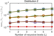
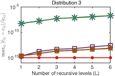
Figure 3: Relative error of Strassen’s algorithm as a function of the number of recursive steps, $L$, for several scaling techniques. The results in each plot are for matrices ${\bm{\mathbf{{A}}}}$ and ${\bm{\mathbf{{B}}}}$ sampled from different probability distributions. (Top) Stability is well-behaved, and no scaling is necessary for small relative errors. (Middle) The matrices are adversarial and inside-outside or 2-times repeated outside-inside scaling have the smallest relative errors. (Right) The matrices are adversarial and outside, outside-inside, or 2-times repeated outside-inside scaling have the smallest relative errors.

Each iteration of outside or inside scaling is $O(MK+KN+MN)$ flops, so scaling does not affect the asymptotic performance. However, quadratic costs do affect the practical implementation of fast matrix multiplication [3]. Subsequently we tested the performance impact of scaling. We use effective gflops [3, 22] to measure the performance of multiplying an $M\times K$ matrix by a $K\times N$ matrix:

(24) $$\frac{2\cdot MKN-MN}{\text{time in seconds}}\cdot\text{1e-9}.$$

This lets us compare fast matrix multiplication algorithms to the classical algorithm on a familiar inverse-time scale. All experiments were conducted on a single compute node on NERSC’s Edison machine. Each node has two 12-core Intel 2.4 GHz Ivy Bridge processors and 64 GB of memory. Our experiments were single-threaded. We report the median of five trials for each timing result.

Fig. 4 summarizes the performance results for Strassen’s algorithm ($L=1$), with and without two steps of Algorithm 3, for multiplying square matrices of dimension $N$. There is a noticeable impact on performance. Strassen’s without scaling out-performs the classical algorithm for $N\geq 2500$ while scaling pushes this threshold to $N\geq 3500$. As $N$ grows, the performance impact of scaling gets smaller. This follows from the asymptotic analysis—as $N$ grows, the impact from quadratic terms shrinks.

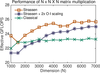
Figure 4: Performance of Strassen’s algorithm ($L=1$), with and without two steps of inside-outside scaling, and the classical algorithm.

7 Discussion

One of the central components of our algorithmic error analysis is that two data-independent quantities drive the error bounds for fast matrix multiplication. First, $Q$ captures the accumulation error from adding matrices. Second, $E$ bounds the growth in the magnitude of intermediate terms. Our results in Section 5 show that having a small $E$ is important, but this does not fully characterize stability in practice. The same result has been observed when comparing Strassen’s algorithm and the Winograd variant [16]. An encouraging result from our experiments is that the number of non-zeroes in the ${\bm{\mathbf{{U}}}}$, ${\bm{\mathbf{{V}}}}$, and ${\bm{\mathbf{{W}}}}$ matrices, which determines the constant in the computational complexity, is positively correlated with $E$. In other words, for a given base case and algorithm rank, by improving performance, we generally also improve stability. Another lesson from our analysis is that we should not think of using fast algorithms asymptotically but rather as having a fixed number of recursive levels. This leads to better performance in practice [3] and also to the improved error bounds and numerical stability presented in Sections 4 and 5. Finally, because the principal quantities for understanding algorithmic error ($E$ and $Q$) are independent of the asymptotic complexity, we have new metrics over which to optimize when searching for fast matrix multiplication algorithms.

For performance reasons, the best choice of fast algorithm depends on the shape of the matrices being multiplied [3]. In general, a choice of algorithm can be made at each recursive level. Subsequently, we believe that uniform non-stationary algorithms are the right choice in practice for achieving the best performance. Theorem 4.6 provides the appropriate error bounds for this case.

The analysis in Section 4.5 formalizes the error analysis for existing techniques to improve stability of Strassen’s algorithm and the Winograd variant [8, 9] and also generalizes the approach for all fast matrix multiplication algorithms. The analysis provides the formula over which to optimize when considering non-uniform, non-stationary algorithms. However, finding the best algorithm is a combinatorial optimization problem that grows exponentially in the number of recursive levels. Algorithm design in this space is an interesting avenue for future research.

Using these algorithmic techniques improves the normwise accuracy of the computed product. However, because the errors are normwise, small elements of the product can be computed less accurately than warranted by their condition numbers. By pre- and post-processing the data, we can improve componentwise accuracy as well. Specifically, we analyzed a hierarchy of diagonal scaling techniques that reduce the number of cases where fast matrix multiplication yields relatively inaccurate small entries in the product. Nevertheless, there are cases that cannot be solved by our diagonal scaling algorithms (e.g., Example 6.15). When scaling helps, a couple of iterations are sufficient, and this is backed up by Theorem 6.9.

The asymptotic operation cost of diagonal scaling is proportional to the size of the matrices, so it is dominated by cost of current matrix multiplication algorithms. In our experiments, we found that scaling does incur a noticeable performance penalty for reasonably sized matrices, but fast matrix multiplication with diagonal scaling still can outperform the classical algorithm. We note that our diagonal scaling implementation is not fully optimized; for example, it is possible to overlap inside and outside scaling and delay updating actual matrix entries, which can both reduce the memory traffic overhead.

Appendix A Strassen’s Algorithm

Strassen’s algorithm [25] is a $\left\langle 2,2,2\right\rangle$ algorithm specified by the following ${\bm{\mathbf{{U}}}}$, ${\bm{\mathbf{{V}}}}$, and ${\bm{\mathbf{{W}}}}$ matrices:

$${\bm{\mathbf{{U}}}} =\begin{bmatrix}\phantom{-}1&\phantom{-}0&\phantom{-}1&\phantom{-}0&\phantom{-}1&-1&\phantom{-}0\phantom{-}\\ \phantom{-}0&\phantom{-}0&\phantom{-}0&\phantom{-}0&\phantom{-}1&\phantom{-}0&\phantom{-}1\phantom{-}\\ \phantom{-}0&\phantom{-}1&\phantom{-}0&\phantom{-}0&\phantom{-}0&\phantom{-}1&\phantom{-}0\phantom{-}\\ \phantom{-}1&\phantom{-}1&\phantom{-}0&\phantom{-}1&\phantom{-}0&\phantom{-}0&-1\phantom{-}\\ \end{bmatrix}$$

$${\bm{\mathbf{{V}}}} =\begin{bmatrix}\phantom{-}1&\phantom{-}1&\phantom{-}0&-1&\phantom{-}0&\phantom{-}1&\phantom{-}0\phantom{-}\\ \phantom{-}0&\phantom{-}0&\phantom{-}1&\phantom{-}0&\phantom{-}0&\phantom{-}1&\phantom{-}0\phantom{-}\\ \phantom{-}0&\phantom{-}0&\phantom{-}0&\phantom{-}1&\phantom{-}0&\phantom{-}0&\phantom{-}1\phantom{-}\\ \phantom{-}1&\phantom{-}0&-1&\phantom{-}0&\phantom{-}1&\phantom{-}0&\phantom{-}1\phantom{-}\\ \end{bmatrix}$$

$${\bm{\mathbf{{W}}}} =\begin{bmatrix}\phantom{-}1&\phantom{-}0&\phantom{-}0&\phantom{-}1&-1&\phantom{-}0&\phantom{-}1\phantom{-}\\ \phantom{-}0&\phantom{-}1&\phantom{-}0&\phantom{-}1&\phantom{-}0&\phantom{-}0&\phantom{-}0\phantom{-}\\ \phantom{-}0&\phantom{-}0&\phantom{-}1&\phantom{-}0&\phantom{-}1&\phantom{-}0&\phantom{-}0\phantom{-}\\ \phantom{-}1&-1&\phantom{-}1&\phantom{-}0&\phantom{-}0&\phantom{-}1&\phantom{-}0\phantom{-}\\ \end{bmatrix}.$$

Note that the rows of ${\bm{\mathbf{{U}}}}$ and ${\bm{\mathbf{{V}}}}$ correspond to a column-major ordering of the entries of the input matrices and the rows of ${\bm{\mathbf{{W}}}}$ correspond to a row-major ordering of the output matrix, following the convention of previous work [6, 17]. We point out that this algorithm is cyclic-invariant, so that (up to permutations on the columns of the matrices), which implies that all three rotations have the same $Q$ and $E$ values.

Appendix B $\left\langle 3,2,3\right\rangle$ fast matrix multiplication algorithm

The following algorithm for base case $\left\langle 3,2,3\right\rangle$ has 94 nonzeros with $E=20$ and $Q=10$.

$${\bm{\mathbf{{U}}}} =\scalebox{0.95}{$\setcounter{MaxMatrixCols}{15}\begin{bmatrix}\phantom{-}0&\phantom{-}1&\phantom{-}0&\phantom{-}0&-1&\phantom{-}1&\phantom{-}1&\phantom{-}0&\phantom{-}0&\phantom{-}0&-1&\phantom{-}0&\phantom{-}0&\phantom{-}0&-1\phantom{-}\\ \phantom{-}0&\phantom{-}1&\phantom{-}0&\phantom{-}0&\phantom{-}0&\phantom{-}0&\phantom{-}0&-1&\phantom{-}0&-1&\phantom{-}0&\phantom{-}0&\phantom{-}1&-1&\phantom{-}0\phantom{-}\\ \phantom{-}0&\phantom{-}0&\phantom{-}0&\phantom{-}1&\phantom{-}0&\phantom{-}0&\phantom{-}0&-1&\phantom{-}0&-1&\phantom{-}1&\phantom{-}0&\phantom{-}0&-1&\phantom{-}0\phantom{-}\\ -1&\phantom{-}0&\phantom{-}1&\phantom{-}0&\phantom{-}1&\phantom{-}0&\phantom{-}0&\phantom{-}0&\phantom{-}0&\phantom{-}0&\phantom{-}1&\phantom{-}0&\phantom{-}0&\phantom{-}0&\phantom{-}1\phantom{-}\\ -1&\phantom{-}0&\phantom{-}0&\phantom{-}0&\phantom{-}0&\phantom{-}1&\phantom{-}0&\phantom{-}1&\phantom{-}0&\phantom{-}1&\phantom{-}0&\phantom{-}1&-1&\phantom{-}0&\phantom{-}0\phantom{-}\\ \phantom{-}0&\phantom{-}0&-1&\phantom{-}0&\phantom{-}0&\phantom{-}0&\phantom{-}0&\phantom{-}1&\phantom{-}1&\phantom{-}0&-1&\phantom{-}0&\phantom{-}0&\phantom{-}0&-1\phantom{-}\\ \end{bmatrix}$}$$

$${\bm{\mathbf{{V}}}} =\scalebox{0.95}{$\setcounter{MaxMatrixCols}{15}\begin{bmatrix}\phantom{-}0&\phantom{-}0&\phantom{-}1&\phantom{-}1&\phantom{-}0&\phantom{-}0&\phantom{-}0&\phantom{-}0&\phantom{-}0&\phantom{-}0&\phantom{-}1&\phantom{-}0&\phantom{-}0&\phantom{-}1&\phantom{-}1\phantom{-}\\ \phantom{-}0&\phantom{-}0&\phantom{-}1&\phantom{-}0&\phantom{-}0&\phantom{-}0&\phantom{-}0&-1&\phantom{-}1&-1&\phantom{-}0&\phantom{-}0&\phantom{-}0&\phantom{-}1&\phantom{-}0\phantom{-}\\ \phantom{-}0&-1&\phantom{-}0&\phantom{-}0&\phantom{-}0&\phantom{-}1&\phantom{-}0&\phantom{-}0&\phantom{-}0&\phantom{-}1&\phantom{-}0&\phantom{-}1&\phantom{-}1&-1&\phantom{-}0\phantom{-}\\ -1&\phantom{-}0&\phantom{-}0&\phantom{-}0&\phantom{-}0&\phantom{-}0&\phantom{-}0&\phantom{-}1&\phantom{-}0&\phantom{-}1&\phantom{-}0&\phantom{-}1&\phantom{-}0&-1&\phantom{-}0\phantom{-}\\ \phantom{-}0&\phantom{-}1&\phantom{-}1&\phantom{-}0&\phantom{-}0&\phantom{-}0&\phantom{-}1&\phantom{-}0&\phantom{-}0&\phantom{-}0&\phantom{-}1&\phantom{-}0&\phantom{-}0&\phantom{-}0&\phantom{-}1\phantom{-}\\ \phantom{-}1&\phantom{-}0&\phantom{-}1&\phantom{-}0&\phantom{-}1&\phantom{-}1&\phantom{-}1&\phantom{-}0&\phantom{-}0&\phantom{-}0&\phantom{-}0&\phantom{-}0&\phantom{-}0&\phantom{-}0&\phantom{-}1\phantom{-}\\ \end{bmatrix}$}$$

$${\bm{\mathbf{{W}}}} =\scalebox{0.95}{$\setcounter{MaxMatrixCols}{15}\begin{bmatrix}\phantom{-}0&\phantom{-}0&\phantom{-}1&\phantom{-}0&\phantom{-}0&\phantom{-}0&-1&\phantom{-}0&\phantom{-}1&\phantom{-}0&\phantom{-}0&\phantom{-}0&\phantom{-}0&\phantom{-}0&-1\phantom{-}\\ \phantom{-}1&\phantom{-}0&\phantom{-}0&\phantom{-}0&\phantom{-}1&\phantom{-}1&\phantom{-}0&\phantom{-}0&\phantom{-}0&\phantom{-}0&\phantom{-}0&-1&\phantom{-}0&\phantom{-}0&\phantom{-}0\phantom{-}\\ \phantom{-}0&\phantom{-}0&\phantom{-}0&\phantom{-}0&\phantom{-}1&\phantom{-}0&\phantom{-}1&\phantom{-}0&\phantom{-}0&\phantom{-}0&\phantom{-}0&\phantom{-}0&\phantom{-}0&\phantom{-}0&\phantom{-}0\phantom{-}\\ \phantom{-}0&\phantom{-}0&\phantom{-}0&-1&\phantom{-}0&\phantom{-}0&\phantom{-}0&\phantom{-}0&\phantom{-}0&-1&\phantom{-}0&\phantom{-}1&\phantom{-}0&-1&\phantom{-}0\phantom{-}\\ \phantom{-}0&\phantom{-}0&\phantom{-}0&\phantom{-}0&\phantom{-}0&\phantom{-}0&\phantom{-}0&\phantom{-}0&\phantom{-}0&\phantom{-}0&\phantom{-}0&\phantom{-}1&\phantom{-}1&\phantom{-}0&\phantom{-}0\phantom{-}\\ \phantom{-}0&\phantom{-}1&\phantom{-}0&\phantom{-}0&\phantom{-}0&\phantom{-}1&-1&\phantom{-}0&\phantom{-}0&\phantom{-}0&\phantom{-}0&\phantom{-}0&\phantom{-}1&\phantom{-}0&\phantom{-}0\phantom{-}\\ \phantom{-}0&\phantom{-}0&\phantom{-}0&\phantom{-}1&\phantom{-}0&\phantom{-}0&\phantom{-}0&\phantom{-}0&\phantom{-}1&\phantom{-}0&\phantom{-}0&\phantom{-}0&\phantom{-}0&\phantom{-}0&\phantom{-}0\phantom{-}\\ \phantom{-}0&\phantom{-}0&\phantom{-}0&\phantom{-}0&\phantom{-}0&\phantom{-}0&\phantom{-}0&\phantom{-}1&\phantom{-}1&-1&\phantom{-}0&\phantom{-}0&-1&\phantom{-}0&\phantom{-}0\phantom{-}\\ \phantom{-}0&\phantom{-}0&\phantom{-}0&-1&\phantom{-}1&\phantom{-}0&\phantom{-}0&\phantom{-}0&\phantom{-}0&\phantom{-}0&\phantom{-}1&\phantom{-}0&\phantom{-}0&\phantom{-}0&-1\phantom{-}\\ \end{bmatrix}$}.$$

Note that the rows of ${\bm{\mathbf{{U}}}}$ and ${\bm{\mathbf{{V}}}}$ correspond to a column-major ordering of the entries of the input matrices and the rows of ${\bm{\mathbf{{W}}}}$ correspond to a row-major ordering of the output matrix, which implies that is an algorithm for $\left\langle 3,3,2\right\rangle$ and is an algorithm for $\left\langle 2,3,3\right\rangle$.

Appendix C $\left\langle 4,4,2\right\rangle$ fast matrix multiplication algorithm

The following algorithm specifies a rank $26$ fast matrix multiplication algorithm with base case $\left\langle 4,4,2\right\rangle$.

$${\bm{\mathbf{{U}}}} =\frac{1}{2}\scalebox{0.55}{$\setcounter{MaxMatrixCols}{26}\begin{bmatrix}\phantom{-}2&\phantom{-}0&\phantom{-}0&-2&\phantom{-}0&\phantom{-}0&\phantom{-}0&\phantom{-}0&-2&\phantom{-}0&\phantom{-}0&\phantom{-}0&\phantom{-}0&-2&\phantom{-}0&\phantom{-}0&\phantom{-}0&\phantom{-}0&\phantom{-}0&\phantom{-}0&\phantom{-}0&\phantom{-}0&\phantom{-}0&\phantom{-}0&\phantom{-}0&\phantom{-}0\\ \phantom{-}0&\phantom{-}0&\phantom{-}0&\phantom{-}0&\phantom{-}0&-2&\phantom{-}0&\phantom{-}0&\phantom{-}0&\phantom{-}0&\phantom{-}2&\phantom{-}2&\phantom{-}2&\phantom{-}0&\phantom{-}0&\phantom{-}0&\phantom{-}0&\phantom{-}0&\phantom{-}0&\phantom{-}0&\phantom{-}0&\phantom{-}0&\phantom{-}0&\phantom{-}0&\phantom{-}0&\phantom{-}0\\ \phantom{-}0&\phantom{-}0&\phantom{-}2&\phantom{-}0&\phantom{-}0&-2&\phantom{-}0&\phantom{-}0&\phantom{-}0&\phantom{-}0&\phantom{-}2&\phantom{-}2&\phantom{-}2&-2&\phantom{-}0&\phantom{-}0&\phantom{-}0&\phantom{-}0&\phantom{-}0&\phantom{-}0&-2&\phantom{-}0&\phantom{-}0&\phantom{-}2&\phantom{-}0&\phantom{-}0\\ \phantom{-}0&\phantom{-}0&\phantom{-}0&\phantom{-}0&\phantom{-}0&\phantom{-}0&\phantom{-}0&\phantom{-}0&\phantom{-}0&\phantom{-}0&\phantom{-}0&-2&\phantom{-}0&\phantom{-}2&\phantom{-}0&\phantom{-}0&\phantom{-}0&\phantom{-}0&\phantom{-}0&\phantom{-}0&\phantom{-}0&\phantom{-}0&\phantom{-}0&\phantom{-}0&\phantom{-}0&\phantom{-}0\\ \phantom{-}0&\phantom{-}2&\phantom{-}0&\phantom{-}0&\phantom{-}0&\phantom{-}0&\phantom{-}0&\phantom{-}1&\phantom{-}0&\phantom{-}0&\phantom{-}0&\phantom{-}0&\phantom{-}0&\phantom{-}0&\phantom{-}0&\phantom{-}0&\phantom{-}0&\phantom{-}0&-1&\phantom{-}0&\phantom{-}0&\phantom{-}0&\phantom{-}0&\phantom{-}0&\phantom{-}0&\phantom{-}2\\ \phantom{-}0&\phantom{-}2&\phantom{-}0&\phantom{-}0&\phantom{-}0&\phantom{-}0&\phantom{-}0&\phantom{-}0&\phantom{-}0&\phantom{-}0&\phantom{-}0&\phantom{-}0&-2&\phantom{-}0&\phantom{-}0&\phantom{-}1&\phantom{-}0&\phantom{-}0&\phantom{-}0&\phantom{-}1&\phantom{-}0&-2&\phantom{-}0&\phantom{-}2&-2&\phantom{-}0\\ \phantom{-}0&\phantom{-}2&\phantom{-}0&\phantom{-}0&\phantom{-}0&\phantom{-}0&\phantom{-}0&\phantom{-}1&\phantom{-}0&\phantom{-}0&\phantom{-}0&\phantom{-}0&\phantom{-}0&\phantom{-}0&\phantom{-}0&\phantom{-}0&\phantom{-}0&\phantom{-}0&-1&\phantom{-}0&\phantom{-}0&-2&\phantom{-}0&\phantom{-}0&\phantom{-}0&\phantom{-}0\\ \phantom{-}0&\phantom{-}0&\phantom{-}0&\phantom{-}1&\phantom{-}2&\phantom{-}0&-1&-1&\phantom{-}0&-1&-2&\phantom{-}2&\phantom{-}0&-2&-2&\phantom{-}0&\phantom{-}0&\phantom{-}1&\phantom{-}0&\phantom{-}0&\phantom{-}1&\phantom{-}0&\phantom{-}0&\phantom{-}0&\phantom{-}0&\phantom{-}0\\ \phantom{-}0&\phantom{-}0&\phantom{-}0&\phantom{-}0&\phantom{-}0&\phantom{-}0&\phantom{-}0&\phantom{-}1&\phantom{-}0&\phantom{-}0&\phantom{-}0&\phantom{-}0&\phantom{-}0&\phantom{-}0&\phantom{-}0&-1&\phantom{-}1&\phantom{-}1&\phantom{-}0&\phantom{-}0&\phantom{-}0&\phantom{-}0&\phantom{-}0&\phantom{-}0&\phantom{-}0&\phantom{-}0\\ \phantom{-}0&\phantom{-}2&\phantom{-}0&\phantom{-}0&-2&\phantom{-}0&\phantom{-}0&\phantom{-}0&\phantom{-}0&\phantom{-}0&\phantom{-}0&\phantom{-}0&\phantom{-}0&\phantom{-}0&\phantom{-}0&\phantom{-}1&\phantom{-}0&\phantom{-}0&\phantom{-}0&\phantom{-}1&\phantom{-}0&-2&\phantom{-}2&\phantom{-}0&\phantom{-}2&\phantom{-}0\\ \phantom{-}0&\phantom{-}2&\phantom{-}0&\phantom{-}0&-2&\phantom{-}0&\phantom{-}0&\phantom{-}1&\phantom{-}0&\phantom{-}0&\phantom{-}0&\phantom{-}0&\phantom{-}0&\phantom{-}0&\phantom{-}0&\phantom{-}0&\phantom{-}0&\phantom{-}1&\phantom{-}0&\phantom{-}0&\phantom{-}0&-2&\phantom{-}2&\phantom{-}0&\phantom{-}2&\phantom{-}0\\ \phantom{-}0&\phantom{-}0&\phantom{-}0&\phantom{-}1&\phantom{-}0&\phantom{-}0&-1&-1&\phantom{-}0&\phantom{-}1&\phantom{-}0&\phantom{-}0&\phantom{-}0&\phantom{-}0&\phantom{-}0&\phantom{-}0&\phantom{-}0&-1&\phantom{-}0&\phantom{-}0&-1&\phantom{-}0&\phantom{-}0&\phantom{-}0&\phantom{-}0&\phantom{-}0\\ \phantom{-}0&-2&\phantom{-}0&\phantom{-}0&\phantom{-}0&\phantom{-}0&\phantom{-}0&\phantom{-}0&\phantom{-}2&\phantom{-}0&\phantom{-}0&\phantom{-}0&\phantom{-}0&\phantom{-}0&\phantom{-}0&\phantom{-}1&-1&-1&\phantom{-}1&\phantom{-}0&\phantom{-}0&\phantom{-}0&\phantom{-}0&\phantom{-}0&\phantom{-}0&-2\\ \phantom{-}0&\phantom{-}0&\phantom{-}0&\phantom{-}0&\phantom{-}2&\phantom{-}0&\phantom{-}0&\phantom{-}0&\phantom{-}0&\phantom{-}0&\phantom{-}0&\phantom{-}0&\phantom{-}2&\phantom{-}0&\phantom{-}0&\phantom{-}0&\phantom{-}0&\phantom{-}0&\phantom{-}0&\phantom{-}0&\phantom{-}0&\phantom{-}0&\phantom{-}0&\phantom{-}0&\phantom{-}0&\phantom{-}0\\ \phantom{-}0&\phantom{-}0&\phantom{-}0&\phantom{-}0&\phantom{-}2&\phantom{-}0&\phantom{-}0&\phantom{-}0&\phantom{-}0&\phantom{-}0&\phantom{-}0&\phantom{-}0&\phantom{-}0&\phantom{-}0&\phantom{-}0&\phantom{-}0&\phantom{-}0&-1&\phantom{-}1&\phantom{-}0&\phantom{-}0&\phantom{-}0&\phantom{-}0&\phantom{-}0&-2&\phantom{-}0\\ \phantom{-}0&\phantom{-}0&\phantom{-}0&\phantom{-}0&-2&\phantom{-}0&\phantom{-}0&\phantom{-}0&\phantom{-}0&\phantom{-}0&\phantom{-}2&\phantom{-}0&\phantom{-}0&\phantom{-}2&\phantom{-}2&\phantom{-}0&\phantom{-}0&\phantom{-}0&\phantom{-}0&\phantom{-}0&\phantom{-}0&\phantom{-}0&\phantom{-}0&\phantom{-}0&\phantom{-}0&\phantom{-}0\\ \end{bmatrix}$ }$$

$${\bm{\mathbf{{V}}}} =\frac{1}{2}\scalebox{0.55}{$\setcounter{MaxMatrixCols}{26}\begin{bmatrix}\phantom{-}2&\phantom{-}0&-2&\phantom{-}0&\phantom{-}0&-2&\phantom{-}0&\phantom{-}0&\phantom{-}0&\phantom{-}0&-2&\phantom{-}0&\phantom{-}0&-2&-2&\phantom{-}0&\phantom{-}0&\phantom{-}0&\phantom{-}0&\phantom{-}0&\phantom{-}0&\phantom{-}0&\phantom{-}0&\phantom{-}0&\phantom{-}0&\phantom{-}0\\ \phantom{-}2&\phantom{-}1&\phantom{-}2&\phantom{-}2&\phantom{-}0&\phantom{-}0&\phantom{-}0&\phantom{-}2&\phantom{-}2&\phantom{-}0&\phantom{-}0&\phantom{-}0&\phantom{-}0&\phantom{-}0&\phantom{-}0&\phantom{-}0&\phantom{-}2&-2&-2&\phantom{-}2&\phantom{-}2&\phantom{-}0&\phantom{-}0&-2&\phantom{-}1&\phantom{-}0\\ -2&\phantom{-}0&-2&-2&\phantom{-}0&-2&-2&\phantom{-}0&\phantom{-}0&-2&\phantom{-}0&-2&\phantom{-}0&\phantom{-}0&\phantom{-}0&\phantom{-}0&\phantom{-}0&\phantom{-}0&\phantom{-}0&\phantom{-}0&-2&\phantom{-}0&\phantom{-}0&\phantom{-}0&\phantom{-}0&\phantom{-}0\\ -2&\phantom{-}0&\phantom{-}2&-2&\phantom{-}0&\phantom{-}0&-2&\phantom{-}0&-2&\phantom{-}2&\phantom{-}0&\phantom{-}0&\phantom{-}0&\phantom{-}0&\phantom{-}0&-2&-2&\phantom{-}0&\phantom{-}0&\phantom{-}2&\phantom{-}2&\phantom{-}0&-2&-2&\phantom{-}0&\phantom{-}0\\ \phantom{-}2&\phantom{-}1&-2&\phantom{-}2&\phantom{-}0&\phantom{-}0&\phantom{-}0&\phantom{-}2&\phantom{-}2&\phantom{-}0&\phantom{-}0&\phantom{-}0&\phantom{-}0&\phantom{-}0&\phantom{-}0&\phantom{-}2&\phantom{-}0&\phantom{-}2&\phantom{-}2&\phantom{-}0&-2&\phantom{-}0&\phantom{-}0&\phantom{-}2&-1&\phantom{-}2\\ \phantom{-}2&\phantom{-}1&-2&\phantom{-}2&\phantom{-}0&\phantom{-}2&\phantom{-}0&\phantom{-}2&\phantom{-}2&\phantom{-}0&\phantom{-}2&\phantom{-}0&-2&\phantom{-}0&\phantom{-}2&\phantom{-}2&\phantom{-}0&\phantom{-}2&-2&\phantom{-}0&-2&\phantom{-}0&\phantom{-}0&\phantom{-}2&-1&\phantom{-}0\\ -2&-2&-2&-2&\phantom{-}0&\phantom{-}0&-2&\phantom{-}0&-2&-2&\phantom{-}0&\phantom{-}0&\phantom{-}0&\phantom{-}0&\phantom{-}0&\phantom{-}0&\phantom{-}0&\phantom{-}0&\phantom{-}0&\phantom{-}0&-2&\phantom{-}2&\phantom{-}2&\phantom{-}2&\phantom{-}0&-2\\ -2&\phantom{-}0&-2&-2&-2&\phantom{-}2&-2&\phantom{-}0&-2&-2&\phantom{-}2&\phantom{-}0&-2&\phantom{-}0&\phantom{-}0&\phantom{-}0&\phantom{-}0&\phantom{-}0&\phantom{-}0&\phantom{-}0&-2&\phantom{-}0&-2&\phantom{-}2&-2&\phantom{-}0\\ \end{bmatrix}$ }$$

$${\bm{\mathbf{{W}}}} =\phantom{\frac{1}{2}}\scalebox{0.55}{$\setcounter{MaxMatrixCols}{26}\begin{bmatrix}\phantom{-}1&-1&\phantom{-}0&\phantom{-}1&\phantom{-}0&\phantom{-}0&\phantom{-}1&\phantom{-}1&\phantom{-}0&\phantom{-}0&\phantom{-}0&\phantom{-}0&\phantom{-}0&\phantom{-}0&\phantom{-}0&\phantom{-}1&\phantom{-}1&\phantom{-}0&\phantom{-}0&\phantom{-}1&\phantom{-}0&\phantom{-}1&\phantom{-}0&\phantom{-}0&\phantom{-}0&\phantom{-}1\\ \phantom{-}0&\phantom{-}1&-1&\phantom{-}0&\phantom{-}0&\phantom{-}0&\phantom{-}0&\phantom{-}0&\phantom{-}0&-1&\phantom{-}0&\phantom{-}0&\phantom{-}0&\phantom{-}0&\phantom{-}0&-1&-1&-1&-1&-1&-1&-1&\phantom{-}0&\phantom{-}0&\phantom{-}0&-1\\ \phantom{-}0&-1&\phantom{-}0&\phantom{-}1&\phantom{-}0&\phantom{-}0&\phantom{-}1&\phantom{-}1&-1&\phantom{-}0&\phantom{-}0&\phantom{-}0&\phantom{-}0&\phantom{-}0&\phantom{-}0&\phantom{-}1&-1&\phantom{-}0&\phantom{-}0&\phantom{-}1&\phantom{-}0&\phantom{-}1&\phantom{-}0&\phantom{-}0&\phantom{-}0&\phantom{-}0\\ \phantom{-}0&\phantom{-}0&\phantom{-}0&\phantom{-}0&\phantom{-}0&\phantom{-}0&\phantom{-}0&\phantom{-}0&\phantom{-}0&\phantom{-}1&\phantom{-}0&\phantom{-}0&\phantom{-}0&\phantom{-}0&\phantom{-}0&\phantom{-}1&\phantom{-}1&\phantom{-}1&\phantom{-}0&-1&\phantom{-}1&-1&-1&-1&\phantom{-}1&\phantom{-}0\\ \phantom{-}0&\phantom{-}0&\phantom{-}1&\phantom{-}0&\phantom{-}1&\phantom{-}0&\phantom{-}0&\phantom{-}0&\phantom{-}0&\phantom{-}1&-1&\phantom{-}0&-1&\phantom{-}0&\phantom{-}1&\phantom{-}1&\phantom{-}1&\phantom{-}1&\phantom{-}0&\phantom{-}1&\phantom{-}1&\phantom{-}0&\phantom{-}0&\phantom{-}0&\phantom{-}1&\phantom{-}0\\ \phantom{-}1&\phantom{-}0&-1&\phantom{-}1&\phantom{-}0&\phantom{-}0&\phantom{-}1&\phantom{-}0&\phantom{-}0&-1&\phantom{-}0&\phantom{-}0&\phantom{-}0&-1&\phantom{-}1&\phantom{-}0&\phantom{-}0&\phantom{-}0&\phantom{-}0&\phantom{-}0&-1&\phantom{-}0&\phantom{-}0&\phantom{-}0&\phantom{-}0&\phantom{-}0\\ \phantom{-}0&\phantom{-}0&\phantom{-}0&\phantom{-}0&-1&\phantom{-}1&\phantom{-}0&\phantom{-}0&\phantom{-}0&-1&\phantom{-}1&\phantom{-}0&\phantom{-}0&\phantom{-}0&-1&-1&-1&-1&\phantom{-}0&\phantom{-}1&-1&\phantom{-}0&\phantom{-}0&\phantom{-}1&-1&\phantom{-}0\\ \phantom{-}0&\phantom{-}0&\phantom{-}0&\phantom{-}0&\phantom{-}0&\phantom{-}1&\phantom{-}1&\phantom{-}0&\phantom{-}0&\phantom{-}1&\phantom{-}1&\phantom{-}1&\phantom{-}0&\phantom{-}0&-1&\phantom{-}0&\phantom{-}0&\phantom{-}0&\phantom{-}0&\phantom{-}0&\phantom{-}0&\phantom{-}0&\phantom{-}0&\phantom{-}0&\phantom{-}0&\phantom{-}0\\ \end{bmatrix}$ }.$$

Note that the rows of ${\bm{\mathbf{{U}}}}$ and ${\bm{\mathbf{{V}}}}$ correspond to a column-major ordering of the entries of the input matrices and the rows of ${\bm{\mathbf{{W}}}}$ correspond to a row-major ordering of the output matrix, which implies that is an algorithm for $\left\langle 4,2,4\right\rangle$ and is an algorithm for $\left\langle 2,4,4\right\rangle$. However, yields an $E=102$, which is greater than ’s 89. The $E$ value can be maintained for base case $\left\langle 2,4,4\right\rangle$ by using a different transformation that corresponds to transposing the matrix multiplication: , where ${\bm{\mathbf{{\cal P}}}}_{m,n}$ is the so-called vec permutation matrix [15], exchanging column-ordering for row-ordering for a vectorized $m\times n$ matrix.

Appendix D Convergence analysis of alternating scaling

In this appendix we prove Theorem 6.9. We start with its first part.

Lemma D.1.

The sequence

$${{r}}^{(t)}_{i}{{s}}^{(t)}_{j}\lVert{\bm{\mathbf{{A\!}}}}^{(t)}\rVert\lVert{\bm{\mathbf{{B}}}}^{(t)}\rVert\qquad\text{for $t=0,1,\dotsc$}$$

is monotonically nonincreasing.

Proof D.2.

If step $t$ is an O step, then

$$\lVert{\bm{\mathbf{{A\!}}}}^{(t)}\rVert=\lVert{\bm{\mathbf{{B}}}}^{(t)}\rVert =1\,, {{r}}^{(t)}_{i} ={{r}}^{(t-1)}_{i}\lVert{{a}}^{(t-1)}_{i,:}\rVert\,, {{s}}^{(t)}_{j} ={{s}}^{(t-1)}_{j}\lVert{{b}}^{(t-1)}_{:,j}\rVert\,,$$

and therefore

$${{r}}^{(t)}_{i}{{s}}^{(t)}_{j}\lVert{\bm{\mathbf{{A\!}}}}^{(t)}\rVert\lVert{\bm{\mathbf{{B}}}}^{(t)}\rVert ={{r}}^{(t-1)}_{i}{{s}}^{(t-1)}_{j}\lVert{{a}}^{(t-1)}_{i,:}\rVert\lVert{{b}}^{(t-1)}_{:,j}\rVert$$

$$\leq{{r}}^{(t-1)}_{i}{{s}}^{(t-1)}_{j}\lVert{\bm{\mathbf{{A\!}}}}^{(t-1)}\rVert\lVert{\bm{\mathbf{{B}}}}^{(t-1)}\rVert\,.$$

Next, assume that step $t$ is an I step. Column $k$ of ${\bm{\mathbf{{A}}}}^{\prime}$ is transformed so that

$${{a}}^{(t)}_{ik} =\left\lparen\frac{\lVert{{b}}^{(t-1)}_{k,:}\rVert}{\lVert{{a}}^{(t-1)}_{:,k}\rVert}\right\rparen^{\!\!\frac{1}{2}}{{a}}^{(t-1)}_{ik}\,,$$

and therefore

(25) $$\lVert{{a}}^{(t)}_{:,k}\rVert =\left\lparen\frac{\lVert{{b}}^{(t-1)}_{k,:}\rVert}{\lVert{{a}}^{(t-1)}_{:,k}\rVert}\right\rparen^{\!\!\frac{1}{2}}\!\lVert{{a}}^{(t-1)}_{:,k}\rVert=\sqrt{\lVert{{a}}^{(t-1)}_{:,k}\rVert\lVert{{b}}^{(t-1)}_{k,:}\rVert}\,,$$

and similarly

(26) $$\lVert{{b}}^{(t)}_{k,:}\rVert =\sqrt{\lVert{{a}}^{(t-1)}_{:,k}\rVert\lVert{{b}}^{(t-1)}_{k,:}\rVert}\,.$$

Hence,

$$\lVert{\bm{\mathbf{{A\!}}}}^{(t)}\rVert=\lVert{\bm{\mathbf{{B}}}}^{(t)}\rVert =\max_{k}\sqrt{\lVert{{a}}^{(t-1)}_{:,k}\rVert\lVert{{b}}^{(t-1)}_{k,:}\rVert}\,, {{r}}^{(t)}_{i} ={{r}}^{(t-1)}_{i}\,, {{s}}^{(t)}_{j} ={{s}}^{(t-1)}_{j}\,,$$

and therefore

$${{r}}^{(t)}_{i}{{s}}^{(t)}_{j}\lVert{\bm{\mathbf{{A\!}}}}^{(t)}\rVert\lVert{\bm{\mathbf{{B}}}}^{(t)}\rVert ={{r}}^{(t-1)}_{i}{{s}}^{(t-1)}_{j}\Big{\lparen}\max_{k}\sqrt{\lVert{{a}}^{(t-1)}_{:,k}\rVert\lVert{{b}}^{(t-1)}_{k,:}\rVert}\,\Big{\rparen}^{2}$$

$$={{r}}^{(t-1)}_{i}{{s}}^{(t-1)}_{j}\max_{k}\bigl{(}\lVert{{a}}^{(t-1)}_{:,k}\rVert\lVert{{b}}^{(t-1)}_{k,:}\rVert\bigr{)}$$

$$\leq{{r}}^{(t-1)}_{i}{{s}}^{(t-1)}_{j}\lVert{\bm{\mathbf{{A\!}}}}^{(t-1)}\rVert\lVert{\bm{\mathbf{{B}}}}^{(t-1)}\rVert\,.$$

Next, we prove that the factors in the sequence of Theorem 6.9 converge individually. This is required in the subsequent analysis.

Lemma D.3.

The sequences ${{r}}^{(t)}_{i}$, ${{s}}^{(t)}_{j}$, $\lVert{\bm{\mathbf{{A\!}}}}^{(t)}\rVert$ and $\lVert{\bm{\mathbf{{B}}}}^{(t)}\rVert$ for $t=0,1,\dotsc$ converge.

Proof D.4.

As we show in the proof of Lemma D.1,

$$\lVert{\bm{\mathbf{{A\!}}}}^{(t)}\rVert=\lVert{\bm{\mathbf{{B}}}}^{(t)}\rVert =1\,,$$

$$\lVert{\bm{\mathbf{{A\!}}}}^{(t+1)}\rVert=\lVert{\bm{\mathbf{{B}}}}^{(t+1)}\rVert =\max_{k}\sqrt{\lVert{{a}}^{(t)}_{:,k}\rVert\lVert{{b}}^{(t)}_{k,:}\rVert} \text{for $t=t_{0},t_{0}+2,\dotsc$}\,.$$

Therefore

$$\lVert{\bm{\mathbf{{A\!}}}}^{(t+1)}\rVert=\max_{k}\sqrt{\lVert{{a}}^{(t)}_{:,k}\rVert\lVert{{b}}^{(t)}_{k,:}\rVert}\leq\sqrt{\lVert{\bm{\mathbf{{A\!}}}}^{(t)}\rVert\lVert{\bm{\mathbf{{B}}}}^{(t)}\rVert}=1\,,$$

and hence

(27) $$r^{\prime(t+2)}_{i}=\lVert{{a}}^{(t+1)}_{i,:}\rVert\leq\lVert{\bm{\mathbf{{A\!}}}}^{(t+1)}\rVert\leq 1\,.$$

The sequence ${{r}}^{(t)}_{i}$ satisfies

$${{r}}^{(t_{0})}_{i} ={{r}}^{(t_{0}+1)}_{i} =r^{\prime(t_{0})}_{i}$$

$${{r}}^{(t_{0}+2)}_{i} ={{r}}^{(t_{0}+3)}_{i} =r^{\prime(t_{0})}_{i}r^{\prime(t_{0}+2)}_{i}$$

$$\mathmakebox[width("{}={}")][c]{\vdots} \mathmakebox[width("{}={}")][c]{\vdots}$$

It is nonnegative because $r^{\prime(t)}_{i}\geq 0$, it is monotonically nonincreasing by Eq. 27, and hence it must converge. The same is true for ${{s}}^{(t)}_{j}$.

Consider the effect of the first $t$ steps of the iteration on ${\bm{\mathbf{{A}}}}^{\prime}$ and ${\bm{\mathbf{{B}}}}^{\prime}$. The cumulative effect of the O steps is to divide the rows of ${\bm{\mathbf{{A}}}}^{\prime}$ by ${{r}}^{(t)}_{i}$ and the columns of ${\bm{\mathbf{{B}}}}^{\prime}$ by ${{s}}^{(t)}_{j}$, and that of the I steps is to make sure that every column of ${\bm{\mathbf{{A}}}}^{\prime}$ is equal in norm to the corresponding row of ${\bm{\mathbf{{B}}}}^{\prime}$. Therefore

$${{a}}^{(t)}_{ik}={{a}}_{ik}\;\frac{1}{{{r}}^{(t)}_{i}}\left\lparen\frac{\max_{j}\big{\lvert}{{b}}_{kj}\big{/}{{s}}^{(t-1)}_{j}\big{\rvert}}{\max_{i}\big{\lvert}{{a}}_{ik}\big{/}{{r}}^{(t-1)}_{i}\big{\rvert}}\right\rparen^{\!\!\frac{1}{2}}\qquad\text{for $t=t_{0}+1,t_{0}+2,\dotsc$}\,,$$

which shows that the convergence of ${{r}}^{(t)}_{i}$ and ${{s}}^{(t)}_{j}$ guarantees the convergence of ${{a}}^{(t)}_{ik}$, and hence also the convergence of $\lVert{\bm{\mathbf{{A\!}}}}^{(t)}\rVert$. The same is true for $\lVert{\bm{\mathbf{{B}}}}^{(t)}\rVert$.

The following Lemma shows that the intermediate scaling factors that we compute in each step rapidly converge to 1. We use the notation

$$w^{(t)} =\max\Big{\lparen}\max_{i}\big{\lvert}\log r^{\prime(t)}_{i}\big{\rvert},\max_{j}\big{\lvert}\log s^{\prime(t)}_{j}\big{\rvert}\Big{\rparen}\,,$$

$$w^{(t+1)} =\max_{k}\big{\lvert}\log p^{\prime(t+1)}_{k}\big{\rvert} \text{for $t=t_{0},t_{0}+2,\dotsc$}\,.$$

Lemma D.5.

The following bounds hold:

$$w^{(t)} \leq w^{(t-1)}\,,$$

$$w^{(t+1)} \leq 0.5w^{(t)} \text{for $t=t_{0}+2,t_{0}+4,\dotsc$}\,.$$

Proof D.6.

Assume that $t=t_{0}+2,t_{0}+4,\dotsc\,.$ Because step $t-2$ is an O step, there is a column $g$ so that $\big{\lvert}{{a}}^{(t-2)}_{ig}\big{\rvert}=1$, and therefore

$$r^{\prime(t)}_{i}=\max_{k}\big{\lvert}{{a}}^{(t-1)}_{ik}\big{\rvert}=\max_{k}\big{\lvert}{{a}}^{(t-2)}_{ik}p^{\prime(t-1)}_{k}\big{\rvert}\geq\big{\lvert}{{a}}^{(t-2)}_{ig}p^{\prime(t-1)}_{g}\big{\rvert}=p^{\prime(t-1)}_{g}\,.$$

Taking logarithms yields

$$\log r^{\prime(t)}_{i} \geq\log p^{\prime(t-1)}_{g}\,.$$

Both sides of this inequality are nonpositive because $$r^{\prime(t)}_{i}\leq 1$$ by Eq. 27, and so

$$\big{\lvert}\log r^{\prime(t)}_{i}\big{\rvert}=-\log r^{\prime(t)}_{i} \leq-\log p^{\prime(t-1)}_{g}=\big{\lvert}\log p^{\prime(t-1)}_{g}\big{\rvert}\,.$$

A similar analysis shows that

$$\big{\lvert}\log s^{\prime(t)}_{j}\big{\rvert} \leq\big{\lvert}\log p^{\prime(t-1)}_{f}\big{\rvert}\,,$$

for a suitably defined row $f$, and these two inequalities imply the first bound in the statement of the Lemma.

Next, let us prove the second bound. We have that

$$\big{\lparen}p^{\prime(t+1)}_{k}\big{\rparen}^{2}=\frac{\max_{j}\big{\lvert}{{b}}^{(t)}_{kj}\big{\rvert}}{\max_{i}\big{\lvert}{{a}}^{(t)}_{ik}\big{\rvert}}=\frac{\max_{j}\big{\lvert}{{b}}^{(t-1)}_{kj}\big{/}s^{\prime(t)}_{j}\big{\rvert}}{\max_{i}\big{\lvert}{{a}}^{(t-1)}_{ik}\big{/}r^{\prime(t)}_{i}\big{\rvert}}\leq\frac{\max_{j}\big{\lvert}{{b}}^{(t-1)}_{kj}\big{\rvert}\;\max_{j}\bigl{(}1\big{/}s^{\prime(t)}_{j}\bigr{)}}{\max_{i}\big{\lvert}{{a}}^{(t-1)}_{ik}\big{/}r^{\prime(t)}_{i}\big{\rvert}}\,.$$

Inequality Eq. 27 states that $r^{\prime(t)}_{i}\leq 1$, and therefore

$$\max_{i}\big{\lvert}{{a}}^{(t-1)}_{ik}\big{/}r^{\prime(t)}_{i}\big{\rvert}\geq\max_{i}\big{\lvert}{{a}}^{(t-1)}_{ik}\big{\rvert}\,,$$

which we substitute into the previous inequality, obtaining

$$\big{\lparen}p^{\prime(t+1)}_{k}\big{\rparen}^{2}\leq\frac{\max_{j}\big{\lvert}{{b}}^{(t-1)}_{kj}\big{\rvert}\;\max_{j}\bigl{(}1\big{/}s^{\prime(t)}_{j}\bigr{)}}{\max_{i}\big{\lvert}{{a}}^{(t-1)}_{ik}\big{\rvert}}\,.$$

By Eqs. 25 and 26

$$\max_{i}\big{\lvert}{{a}}^{(t-1)}_{ik}\big{\rvert}=\lVert{{a}}^{(t-1)}_{:,k}\rVert=\lVert{{b}}^{(t-1)}_{k,:}\rVert=\max_{j}\big{\lvert}{{b}}^{(t-1)}_{kj}\big{\rvert}\,,$$

which implies

$$\big{\lparen}p^{\prime(t+1)}_{k}\big{\rparen}^{2} \leq\max\nolimits_{j}\big{\lparen}1\big{/}s^{\prime(t)}_{j}\big{\rparen}\,.$$

A similar analysis shows that

$$\big{\lparen}p^{\prime(t+1)}_{k}\big{\rparen}^{2} \geq\frac{1}{\max_{i}\big{\lparen}1\big{/}r^{\prime(t)}_{i}\big{\rparen}}\,.$$

Taking the logarithm of these two bounds and interchanging the positions of the logarithms with those of the $\max$ operators yields

$$-\max_{i}\Big{\lparen}\log\big{\lparen}1\big{/}r^{\prime(t)}_{i}\big{\rparen}\Big{\rparen}\leq 2\log p^{\prime(t+1)}_{k}\leq\max_{j}\Big{\lparen}\log\big{\lparen}1\big{/}s^{\prime(t)}_{j}\big{\rparen}\Big{\rparen}\,.$$

Because $r^{\prime(t)}_{i}\leq 1$ we have that $\log\big{\lparen}1\big{/}r^{\prime(t)}_{i}\big{\rparen}=\big{\lvert}\log r^{\prime(t)}_{i}\big{\rvert}$, and similarly for $s^{\prime(t)}_{j}$. Applying this to the previous inequality yields

$$-\max_{i}\big{\lvert}\log r^{\prime(t)}_{i}\big{\rvert}\leq 2\log p^{\prime(t+1)}_{k}\leq\max_{j}\big{\lvert}\log s^{\prime(t)}_{j}\big{\rvert}\,,$$

and therefore

$$2\big{\lvert}\log p^{\prime(t+1)}_{k}\big{\rvert}\leq\max\Big{\lparen}\max_{i}\big{\lvert}\log r^{\prime(t)}_{i}\big{\rvert},\max_{j}\big{\lvert}\log s^{\prime(t)}_{j}\big{\rvert}\Big{\rparen}\,,$$

which implies the second bound in the statement of the Lemma.

The following lemma proves linear convergence, and therefore completes the proof of Theorem 6.9.

Lemma D.7.

There is a sequence $\nu^{(t)}$ so that

$${{\mu}}^{(t)}_{ij} \leq\nu^{(t)}\,, {{\mu}}^{(t+1)}_{ij} \leq\nu^{(t+1)}\,,$$

and

$$\nu^{(t+1)} =\nu^{(t)}\,, \nu^{(t+2)} \leq 0.5\,\nu^{(t)} t=t_{0},t_{0}+2,\dotsc.$$ for

Proof D.8.

Assume that $t=t_{0},t_{0}+2,\dotsc.$ Rearranging the definition of ${{\mu}}^{(t)}_{ij}$, we may write

$${{\mu}}^{(t)}_{ij}=\big{\lparen}{{r}}^{(t)}_{i}{{s}}^{(t)}_{j}\lVert{\bm{\mathbf{{A\!}}}}^{(t)}\rVert\lVert{\bm{\mathbf{{B}}}}^{(t)}\rVert\big{\rparen}\,\big{\lparen}{{r}}^{(\star)}_{i}{{s}}^{(\star)}_{j}\lVert{\bm{\mathbf{{A\!}}}}^{(\star)}\rVert\lVert{\bm{\mathbf{{B}}}}^{(\star)}\rVert\big{\rparen}^{-1}-1\,.$$

We have that

$${{r}}^{(t)}_{i} =r^{\prime(t_{0})}_{i}r^{\prime(t_{0}+2)}_{i}\dotsm r^{\prime(t)}_{i}\,, {{s}}^{(t)}_{j} =s^{\prime(t_{0})}_{j}s^{\prime(t_{0}+2)}_{j}\dotsm s^{\prime(t)}_{j}\,, \lVert{\bm{\mathbf{{A\!}}}}^{(t)}\rVert=\lVert{\bm{\mathbf{{B}}}}^{(t)}\rVert =1\,,$$

and therefore

$${{r}}^{(\star)}_{i} =r^{\prime(t_{0})}_{i}r^{\prime(t_{0}+2)}_{i}\dotsm\,, {{s}}^{(\star)}_{j} =s^{\prime(t_{0})}_{j}s^{\prime(t_{0}+2)}_{j}\dotsm\,, \lVert{\bm{\mathbf{{A\!}}}}^{(\star)}\rVert=\lVert{\bm{\mathbf{{B}}}}^{(\star)}\rVert =1\,.$$

Substituting this into the above yields

$${{\mu}}^{(t)}_{ij} =\big{\lparen}r^{\prime(t_{0})}_{i}s^{\prime(t_{0})}_{j}r^{\prime(t_{0}+2)}_{i}s^{\prime(t_{0}+2)}_{j}\dotsm r^{\prime(t)}_{i}s^{\prime(t)}_{j}\big{\rparen}\,\big{\lparen}r^{\prime(t_{0})}_{i}s^{\prime(t_{0})}_{j}r^{\prime(t_{0}+2)}_{i}s^{\prime(t_{0}+2)}_{j}\dotsm\big{\rparen}^{-1}-1$$

$$=\big{\lparen}r^{\prime(t+2)}_{i}s^{\prime(t+2)}_{j}r^{\prime(t+4)}_{i}s^{\prime(t+4)}_{j}\dotsm\big{\rparen}^{-1}-1\,.$$

Applying the definition of $w^{(t)}$ to this, we obtain

$${{\mu}}^{(t)}_{ij} =\big{\lparen}r^{\prime(t+2)}_{i}s^{\prime(t+2)}_{j}r^{\prime(t+4)}_{i}s^{\prime(t+4)}_{j}\dotsm\big{\rparen}^{-1}-1$$

$$=\exp\big{\lparen}-\log r^{\prime(t+2)}_{i}-\log s^{\prime(t+2)}_{j}-\log r^{\prime(t+4)}_{i}-\log s^{\prime(t+4)}_{j}-\dotsb\big{\rparen}-1$$

$$=\exp\big{\lparen}\big{\lvert}\log r^{\prime(t+2)}_{i}\big{\rvert}+\big{\lvert}\log s^{\prime(t+2)}_{j}\big{\rvert}+\big{\lvert}\log r^{\prime(t+4)}_{i}\big{\rvert}+\big{\lvert}\log s^{\prime(t+4)}_{j}\big{\rvert}+\dotsb\big{\rparen}-1$$

$$\leq\exp\big{\lparen}2w^{(t+2)}+2w^{(t+4)}+\dotsb\big{\rparen}-1\,.$$

We define

$$\nu^{(t)}=\exp\big{\lparen}2w^{(t+2)}+2w^{(t+4)}+\dotsb\big{\rparen}-1\,,\qquad\nu^{(t+1)}=\nu^{(t)}\,,$$

thereby guaranteeing that ${{\mu}}^{(t)}_{ij}\leq\nu^{(t)}$, as the Lemma states. Since ${{r}}^{(t)}_{i}{{s}}^{(t)}_{j}\lVert{\bm{\mathbf{{A\!}}}}^{(t)}\rVert\lVert{\bm{\mathbf{{B}}}}^{(t)}\rVert$ is monotonically nonincreasing, so is its relative distance to its limit, meaning that

$${{\mu}}^{(t+1)}_{ij} \leq{{\mu}}^{(t)}_{ij}$$

and hence

$${{\mu}}^{(t+1)}_{ij} \leq{{\mu}}^{(t)}_{ij}\leq\nu^{(t)}=\nu^{(t+1)}\,.$$

This proves another condition in the statement of the Lemma, leaving us only with the condition $\nu^{(t+2)}\leq 0.5\,\nu^{(t)}$ to prove.

By Lemma D.5,

$$w^{(t+3)} \leq 0.5w^{(t+2)} w^{(t+4)} \leq w^{(t+3)} \leq 0.5w^{(t+2)}$$

$$w^{(t+5)} \leq 0.5w^{(t+4)} \leq 0.25w^{(t+2)}\qquad w^{(t+6)} \leq w^{(t+5)} \leq 0.25w^{(t+2)}$$

$$\mathmakebox[width("{}\leq{}")][c]{\vdots} \mathmakebox[width("{}\leq{}")][c]{\vdots} \mathmakebox[width("{}\leq{}")][c]{\vdots} \mathmakebox[width("{}\leq{}")][c]{\vdots}$$

Therefore

$$w^{(t+2)} =\lparen 0.5+0.25+\dotsb\rparen w^{(t+2)}$$

$$=0.5w^{(t+2)}+0.25w^{(t+2)}+\dotsb$$

$$\geq w^{(t+4)}+w^{(t+6)}+\dotsb\,,$$

and thus

$$\exp\big{\lparen}2w^{(t+2)}\big{\rparen} \geq\exp\big{\lparen}2w^{(t+4)}+2w^{(t+6)}+\dotsb\big{\rparen}\,.$$

Applying this bound to the definition of $\nu^{(t)}$, we obtain

$$\nu^{(t)} =\exp\big{\lparen}2w^{(t+2)}+2w^{(t+4)}+\dotsb\big{\rparen}-1$$

$$=\exp\big{\lparen}2w^{(t+2)}\big{\rparen}\exp\big{\lparen}2w^{(t+4)}+2w^{(t+6)}+\dotsb\big{\rparen}-1$$

$$\geq\Big{\lparen}\exp\big{\lparen}2w^{(t+4)}+2w^{(t+6)}+\dotsb\big{\rparen}\Big{\rparen}^{2}-1\,.$$

We define $x=\exp\big{\lparen}2w^{(t+4)}+2w^{(t+6)}+\dotsb\big{\rparen}$, so that the above expression has the form $x^{2}-1$ and $\nu^{(t+2)}=x-1$. The rest of the proof is:

$$\nu^{(t)}\geq x^{2}-1=\lparen 2+x-1\rparen\lparen x-1\rparen=\big{\lparen}2+\nu^{(t+2)}\big{\rparen}\,\nu^{(t+2)}\geq 2\,\nu^{(t+2)}\,,$$

which implies that $\nu^{(t+2)}\leq 0.5\,\nu^{(t)}$ as the Lemma states.

Finally, we show that the analysis in Lemma D.7 is asymptotically sharp.

Lemma D.9.

There are matrices ${\bm{\mathbf{{A}}}}$ and ${\bm{\mathbf{{B}}}}$ and indices $i$ and $j$ so that

$${{\mu}}^{(t+1)}_{ij}={{\mu}}^{(t)}_{ij}\,,\qquad{{\mu}}^{(t+2)}_{ij}\big{/}{{\mu}}^{(t)}_{ij}\to 0.5\qquad\text{for $t=t_{0},t_{0}+2,\dotsc.$}$$

Proof D.10.

Let

$${\bm{\mathbf{{A}}}}=\begin{bmatrix}1&0\\ 1&2^{-2^{v}}\end{bmatrix}\,,\qquad{\bm{\mathbf{{B}}}}=\begin{bmatrix}1&0\\ 0&1\end{bmatrix}$$

for some integer $v$, let us start the iteration with an O step, and assume that $t=t_{0},t_{0}+2,\dotsc.$ A straightforward calculation, which we omit for brevity, shows that

$${\bm{\mathbf{{A\!}}}}^{(t)} =\begin{bmatrix}1&0\\ 1&2^{-2^{v-(t-t_{0})/2}}\end{bmatrix}\,, \begin{bmatrix}{{r}}^{(t)}_{1}\\ {{r}}^{(t)}_{2}\end{bmatrix} =\begin{bmatrix}\vphantom{{{r}}^{(t)}_{1}}1\\ \vphantom{{{r}}^{(t)}_{2}}1\end{bmatrix}\,,$$

$${\bm{\mathbf{{B}}}}^{(t)} =\begin{bmatrix}1&0\\ 0&1\end{bmatrix}\,, \begin{bmatrix}{{s}}^{(t)}_{1}\\ {{s}}^{(t)}_{2}\end{bmatrix} =\begin{bmatrix}[l]\vphantom{{{s}}^{(t)}_{1}}1\\ \vphantom{{{s}}^{(t)}_{2}}2^{-2^{v}(1-2^{-(t-t_{0})/2})}\end{bmatrix}\,,$$

$${\bm{\mathbf{{A\!}}}}^{(t+1)} =\begin{bmatrix}1&0\\ 1&2^{-2^{v-(t-t_{0})/2-1}}\end{bmatrix}\,, \begin{bmatrix}{{r}}^{(t+1)}_{1}\\ {{r}}^{(t+1)}_{2}\end{bmatrix} =\begin{bmatrix}{{r}}^{(t)}_{1}\\ {{r}}^{(t)}_{2}\end{bmatrix}\,,$$

$${\bm{\mathbf{{B}}}}^{(t+1)} =\begin{bmatrix}1&0\\ 0&2^{-2^{v-(t-t_{0})/2-1}}\end{bmatrix}\,, \begin{bmatrix}{{s}}^{(t+1)}_{1}\\ {{s}}^{(t+1)}_{2}\end{bmatrix} =\begin{bmatrix}{{s}}^{(t)}_{1}\\ {{s}}^{(t)}_{2}\end{bmatrix}\,,$$

and therefore

$${\bm{\mathbf{{A\!}}}}^{(\star)}=\begin{bmatrix}1&0\\ 1&1\end{bmatrix}\,,\qquad{\bm{\mathbf{{B}}}}^{(\star)}=\begin{bmatrix}1&0\\ 0&1\end{bmatrix}\,,\qquad\begin{bmatrix}{{r}}^{(\star)}_{1}\\ {{r}}^{(\star)}_{2}\end{bmatrix}=\begin{bmatrix}\vphantom{{{r}}^{(\star)}_{1}}1\\ \vphantom{{{r}}^{(\star)}_{2}}1\end{bmatrix}\,,\qquad\begin{bmatrix}{{s}}^{(\star)}_{1}\\ {{s}}^{(\star)}_{2}\end{bmatrix}=\begin{bmatrix}[l]\vphantom{{{s}}^{(\star)}_{1}}1\\ \vphantom{{{s}}^{(\star)}_{2}}2^{-2^{v}}\end{bmatrix}$$

and

$$\lVert{\bm{\mathbf{{A\!}}}}^{(t)}\rVert=\lVert{\bm{\mathbf{{B}}}}^{(t)}\rVert=\lVert{\bm{\mathbf{{A\!}}}}^{(t+1)}\rVert=\lVert{\bm{\mathbf{{B}}}}^{(t+1)}\rVert=\lVert{\bm{\mathbf{{A\!}}}}^{(\star)}\rVert=\lVert{\bm{\mathbf{{B}}}}^{(\star)}\rVert=1\,.$$

Substituting the above into the definition of ${{\mu}}^{(t)}_{ij}$ yields

(28) $${{\mu}}^{(t)}_{22}={{\mu}}^{(t+1)}_{22} =\frac{\big{\lvert}{{r}}^{(t)}_{2}{{s}}^{(t)}_{2}\lVert{\bm{\mathbf{{A\!}}}}^{(t)}\rVert\lVert{\bm{\mathbf{{B}}}}^{(t)}\rVert-{{r}}^{(\star)}_{2}{{s}}^{(\star)}_{2}\lVert{\bm{\mathbf{{A\!}}}}^{(\star)}\rVert\lVert{\bm{\mathbf{{B}}}}^{(\star)}\rVert\big{\rvert}}{\big{\lvert}{{r}}^{(\star)}_{2}{{s}}^{(\star)}_{2}\lVert{\bm{\mathbf{{A\!}}}}^{(\star)}\rVert\lVert{\bm{\mathbf{{B}}}}^{(\star)}\rVert\big{\rvert}}$$

$$=\frac{\big{\lvert}2^{-2^{v}(1-2^{-(t-t_{0})/2})}-2^{-2^{v}}\big{\rvert}}{\big{\lvert}2^{-2^{v}}\big{\rvert}}$$

$$=2^{2^{v-(t-t_{0})/2}}-1\,.$$

Letting $x=2^{2^{v-(t-t_{0})/2-1}}$, so that the above expression has the form $x^{2}-1$ and ${{\mu}}^{(t+2)}_{22}=x-1$, we have that

$${{\mu}}^{(t)}_{22}=x^{2}-1=(2+x-1)(x-1)=\big{\lparen}2+{{\mu}}^{(t+2)}_{22}\big{\rparen}\,{{\mu}}^{(t+2)}_{22}\,,$$

and therefore

$${{\mu}}^{(t+2)}_{22}\big{/}{{\mu}}^{(t)}_{22}=1\big{/}\big{\lparen}2+{{\mu}}^{(t+2)}_{22}\big{\rparen}\;\,.$$

From Eq. 28 we conclude that ${{\mu}}^{(t+2)}_{22}\to 0,$ and therefore ${{\mu}}^{(t+2)}_{22}\big{/}{{\mu}}^{(t)}_{22}\to 0.5.$

Appendix E Proof of Theorem 6.11

Proof E.1.

In the proof of Lemma D.7 (see D), we show that for all $i,j$ and $t=t_{0},t_{0}+2,\dotsc$,

$${{\mu}}^{(t+1)}_{ij} \leq{{\mu}}^{(t)}_{ij}\,,$$

$${{\mu}}^{(t)}_{ij} \leq\exp\big{\lparen}2w^{(t+2)}+2w^{(t+4)}+\dotsb\big{\rparen}-1\,,$$

$$\exp\big{\lparen}2w^{(t+4)}+2w^{(t+6)}+\dotsb\big{\rparen} \leq\exp\big{\lparen}2w^{(t+2)}\big{\rparen}\,.$$

Putting these three statements together yields

$${{\mu}}^{(t+1)}_{ij} \leq{{\mu}}^{(t)}_{ij}\leq\exp\big{\lparen}2w^{(t+2)}+2w^{(t+4)}+\dotsb\big{\rparen}-1$$

$$=\exp\big{\lparen}2w^{(t+2)}\big{\rparen}\exp\big{\lparen}2w^{(t+4)}+2w^{(t+6)}+\dotsb\big{\rparen}-1$$

$$\leq\exp\big{\lparen}2w^{(t+2)}\big{\rparen}\exp\big{\lparen}2w^{(t+2)}\big{\rparen}-1$$

$$=\exp\big{\lparen}4w^{(t+2)}\big{\rparen}-1\,.$$

Lemma D.5 guarantees that $$w^{(t+2)}\leq w^{(t+1)}$$, and substituting this into the above yields

(29) $${{\mu}}^{(t+1)}_{ij} \leq\exp\big{\lparen}4w^{(t+1)}\big{\rparen}-1\,.$$

Similarly,

(30) $${{\mu}}^{(t+2)}_{ij} \leq\exp\big{\lparen}2w^{(t+4)}+2w^{(t+6)}+\dotsb\big{\rparen}-1\leq\exp\big{\lparen}2w^{(t+2)}\big{\rparen}-1\,.$$

Next, let us prove the first statement of the Theorem. Assume that

$$(1+\tau)^{-\frac{1}{4}}\leq p^{\prime(t+1)}_{k}\leq(1+\tau)^{\frac{1}{4}}$$

for all $k$. Taking logarithms yields

$$-0.25\log(1+\tau)\leq\log p^{\prime(t+1)}_{k}\leq 0.25\log(1+\tau)\,,$$

or equivalently

$$\big{\lvert}\log p^{\prime(t+1)}_{k}\big{\rvert}\leq 0.25\log(1+\tau)\,,$$

and therefore

$$w^{(t+1)}=\max_{k}\big{\lvert}\log p^{\prime(t+1)}_{k}\big{\rvert}\leq 0.25\log(1+\tau)\,.$$

Substituting this into Eq. 29, we find that

$${{\mu}}^{(t+1)}_{ij}\leq\exp\big{\lparen}4w^{(t+1)}\big{\rparen}-1\leq\exp\big{\lparen}4\cdot 0.25\log(1+\tau)\big{\rparen}-1=\tau\,,$$

for all $i,j$, which proves the first statement of the Theorem.

Let us prove the second statement of the Theorem. Assume that

$$(1+\tau)^{-\frac{1}{2}}\leq r^{\prime(t+2)}_{i}\,,\qquad(1+\tau)^{-\frac{1}{2}}\leq s^{\prime(t+2)}_{j}\\$$

for all $i$ and $j$. Taking logarithms yields

$$-0.5\log(1+\tau)\leq\log r^{\prime(t+2)}_{i}\,,\qquad-0.5\log(1+\tau)\leq\log s^{\prime(t+2)}_{j}\,.$$

We show in the proof of Lemma D.3 that $r^{\prime(t+2)}_{i}\leq 1$, and therefore $\log r^{\prime(t+2)}_{i}\leq 0$ and similarly for $s^{\prime(t+2)}_{j}$. Hence

$$\big{\lvert}\log r^{\prime(t+2)}_{i}\big{\rvert}\leq 0.5\log(1+\tau)\,,\qquad\big{\lvert}\log s^{\prime(t+2)}_{j}\big{\rvert}\leq 0.5\log(1+\tau)\,,$$

and hence

$$w^{(t+2)}=\max\Big{\lparen}\max_{i}\big{\lvert}\log r^{\prime(t+2)}_{i}\big{\rvert},\max_{j}\big{\lvert}\log s^{\prime(t+2)}_{j}\big{\rvert}\Big{\rparen}\leq 0.5\log(1+\tau)\,.$$

Substituting this into Eq. 30 yields

$${{\mu}}^{(t+2)}_{ij}\leq\exp\big{\lparen}2w^{(t+2)}\big{\rparen}-1\leq\exp\big{\lparen}2\cdot 0.5\log(1+\tau)\big{\rparen}-1=\tau\,,$$

for all $i,j$, which proves the second statement of the Theorem.

References

• [1] G. Ballard, J. Demmel, O. Holtz, B. Lipshitz, and O. Schwartz, Communication-optimal parallel algorithm for Strassen’s matrix multiplication, in Proceedings of the 24th ACM Symposium on Parallelism in Algorithms and Architectures, ACM, 2012, pp. 193–204.
• [2] G. Ballard, J. Demmel, O. Holtz, and O. Schwartz, Graph expansion and communication costs of fast matrix multiplication, in Proceedings of the 23rd ACM Symposium on Parallelism in Algorithms and Architectures, SPAA ’11, ACM, 2011, pp. 1–12, http://doi.acm.org/10.1145/1989493.1989495.
• [3] A. R. Benson and G. Ballard, A framework for practical parallel fast matrix multiplication, in Proceedings of the 20th ACM SIGPLAN Symposium on Principles and Practice of Parallel Programming, PPoPP 2015, ACM, 2015, pp. 42–53, doi:10.1145/2688500.2688513, http://doi.acm.org/10.1145/2688500.2688513.
• [4] D. Bini and G. Lotti, Stability of fast algorithms for matrix multiplication, Numerische Mathematik, 36 (1980), pp. 63–72.
• [5] M. Bläser, On the complexity of the multiplication of matrices of small formats, Journal of Complexity, 19 (2003), pp. 43–60.
• [6] R. P. Brent, Algorithms for matrix multiplication, tech. report, Stanford University, Stanford, CA, USA, 1970.
• [7] R. P. Brent, Error analysis of algorithms for matrix multiplication and triangular decomposition using Winograd’s identity, Numerische Mathematik, 16 (1970), pp. 145–156.
• [8] R. R. Castrapel and J. L. Gustafson, Precision improvement method for the Strassen/Winograd matrix multiplication method, Apr. 24 2007, http://www.google.com/patents/US7209939. US Patent 7,209,939.
• [9] P. D’Alberto, The better accuracy of Strassen-Winograd algorithms (FastMMW), Advances in Linear Algebra & Matrix Theory, 4 (2014), p. 9.
• [10] L. De Moura and N. Bjørner, Z3: An efficient SMT solver, in Tools and Algorithms for the Construction and Analysis of Systems, Springer, 2008, pp. 337–340.
• [11] J. Demmel, I. Dumitriu, and O. Holtz, Fast linear algebra is stable, Numerische Mathematik, 108 (2007), pp. 59–91.
• [12] J. Demmel, I. Dumitriu, O. Holtz, and R. Kleinberg, Fast matrix multiplication is stable, Numerische Mathematik, (2006).
• [13] B. Dumitrescu, Improving and estimating the accuracy of Strassen’s algorithm, Numerische Mathematik, 79 (1998), pp. 485–499.
• [14] F. L. Gall, Powers of tensors and fast matrix multiplication, in Proceedings of the International Symposium on Symbolic and Algebraic Computation, 2014, pp. 296–303.
• [15] H. V. Henderson and S. R. Searle, The vec-permutation matrix, the vec operator and kronecker products: a review, Linear and Multilinear Algebra, 9 (1981), pp. 271–288, doi:10.1080/03081088108817379, http://dx.doi.org/10.1080/03081088108817379.
• [16] N. J. Higham, Accuracy and stability of numerical algorithms, SIAM, 2002.
• [17] R. W. Johnson and A. M. McLoughlin, Noncommutative bilinear algorithms for 3 x 3 matrix multiplication, SIAM Journal on Computing, 15 (1986), pp. 595–603.
• [18] I. Kaporin, A practical algorithm for faster matrix multiplication, Numerical Linear Algebra with Applications, 6 (1999), pp. 687–700.
• [19] I. Kaporin, The aggregation and cancellation techniques as a practical tool for faster matrix multiplication, Theoretical Computer Science, 315 (2004), pp. 469–510.
• [20] J. Laderman, V. Pan, and X.-H. Sha, On practical algorithms for accelerated matrix multiplication, Linear Algebra and its Applications, 162 (1992), pp. 557–588.
• [21] J. Landsberg, New lower bounds for the rank of matrix multiplication, SIAM Journal on Computing, 43 (2014), pp. 144–149, doi:10.1137/120880276, http://dx.doi.org/10.1137/120880276, arXiv:http://dx.doi.org/10.1137/120880276.
• [22] B. Lipshitz, G. Ballard, J. Demmel, and O. Schwartz, Communication-avoiding parallel Strassen: Implementation and performance, in Proceedings of the International Conference for High Performance Computing, Networking, Storage, and Analysis, 2012.
• [23] W. Miller, Computational complexity and numerical stability, SIAM Journal on Computing, 4 (1975), pp. 97–107.
• [24] A. V. Smirnov, The bilinear complexity and practical algorithms for matrix multiplication, Computational Mathematics and Mathematical Physics, 53 (2013), pp. 1781–1795.
• [25] V. Strassen, Gaussian elimination is not optimal, Numerische Mathematik, 13 (1969), pp. 354–356.