Distributional Smoothing
with Virtual Adversarial Training
Abstract
We propose local distributional smoothness (LDS), a new notion of smoothness for statistical model that can be used as a regularization term to promote the smoothness of the model distribution. We named the LDS based regularization as virtual adversarial training (VAT). The LDS of a model at an input datapoint is defined as the KL-divergence based robustness of the model distribution against local perturbation around the datapoint. VAT resembles adversarial training, but distinguishes itself in that it determines the adversarial direction from the model distribution alone without using the label information, making it applicable to semi-supervised learning. The computational cost for VAT is relatively low. For neural network, the approximated gradient of the LDS can be computed with no more than three pairs of forward and back propagations. When we applied our technique to supervised and semi-supervised learning for the MNIST dataset, it outperformed all the training methods other than the current state of the art method, which is based on a highly advanced generative model. We also applied our method to SVHN and NORB, and confirmed our method’s superior performance over the current state of the art semi-supervised method applied to these datasets.
1 Introduction
Overfitting is a serious problem in supervised training of classification and regression functions. When the number of training samples is finite, training error computed from empirical distribution of the training samples is bound to be different from the test error, which is the expectation of the log-likelihood with respect to the true underlying probability measure Akaike (1998); Watanabe (2009).
One popular countermeasure against overfitting is addition of a regularization term to the objective function. The introduction of the regularization term makes the optimal parameter for the objective function to be less dependent on the likelihood term. In Bayesian framework, the regularization term corresponds to the logarithm of the prior distribution of the parameters, which defines the preference of the model distribution. Of course, there is no universally good model distribution, and the good model distribution should be chosen dependent on the problem we tackle. Still yet, our experiences often dictate that the outputs of good models should be smooth with respect to inputs. For example, images and time series occurring in nature tend to be smooth with respect to the space and time Wahba (1990). We would therefore invent a novel regularization term called local distributional smoothness (LDS), which rewards the smoothness of the model distribution with respect to the input around every input datapoint,
We define LDS as the negative of the sensitivity of the model distribution with respect to the perturbation of , measured in the sense of KL divergence. The objective function based on this regularization term is therefore the log likelihood of the dataset augmented with the sum of LDS computed at every input datapoint in the dataset. Because LDS is measuring the local smoothness of the model distribution itself, the regularization term is parametrization invariant. More precisely, our regularized objective function satisfies the natural property that, if the , then for any diffeomorphism . Therefore, regardless of the parametrization, the optimal model distribution trained with LDS regularization is unique. This is a property that is not enjoyed by the popular regularization Friedman et al. (2001). Also, for sophisticated models like deep neural network Bengio (2009); LeCun et al. (2015), it is not a simple task to assess the effect of the regularization term on the topology of the model distribution.
Our work is closely related to adversarial training Goodfellow et al. (2015). At each step of the training, Goodfellow et al. identified for each pair of the observed input and its label the direction of the input perturbation to which the classifier’s label assignment of is most sensitive. Goodfellow et al. then penalized the model’s sensitivity with respect to the perturbation in the adversarial direction. On the other hand, our LDS defined without label information. Using the language of adversarial training, LDS at each point is therefore measuring the robustness of the model against the perturbation in local and ‘virtual’ adversarial direction. We therefore refer to our regularization method as virtual adversarial training (VAT). Because LDS does not require the label information, VAT is also applicable to semi-supervised learning. This is not the case for adversarial training.
Furthermore, with the second order Taylor expansion of the LDS and an application of power method, we made it possible to approximate the gradient of the LDS efficiently. The approximated gradient of the LDS can be computed with no more than three pairs of forward and back propagations.
We summarize the advantages of our method below:
-
•
Applicability to both supervised and semi-supervised training.
-
•
At most two hyperparameters.
-
•
Parametrization invariant formulation. The performance of the method is invariant under reparatrization of the model.
-
•
Low computational cost. For Neural network in particular, the approximated gradient of the LDS can be computed with no more than three pairs of forward and back propagations.
When we applied the VAT to the supervised and semi-supervised learning of the permutation invariant task for the MNIST dataset, our method outperformed all the contemporary methods other than the state of the art method Rasmus et al. (2015) that uses a highly advanced generative model based method. We also applied our method for semi-supervised learning of permutation invariant task for the SVHN and NORB dataset, and confirmed our method’s superior performance over the current state of the art semi-supervised method applied to these datasets.
2 Methods
2.1 Formalization of Local Distributional Smoothness
We begin with the formal definition of the local distributional smoothness. Let us fix for now, suppose the input space , the output space , and a training samples
and consider the problem of using to train the model distribution parametrized by . Let denote the KL divergence between the distributions and . Also, with the hyperparameter , we define
| (1) | ||||
| (2) |
From now on, we refer to as the virtual adversarial perturbation. We define the local distributional smoothing (LDS) of the model distribution at by
| (3) |
Note is the direction to which the model distribution is most sensitive in the sense of KL divergence. In a way, this is a KL divergence analogue of the gradient of the model distribution with respect to the input, and perturbation of in this direction wrecks the local smoothness of at in a most dire way. The smaller the value of at , the smoother the at . Our goal is to improve the smoothness of the model in the neighborhood of all the observed inputs. Formulating this goal based on the LDS, we obtain the following objective function,
| (4) |
We call the training based on (4) the virtual adversarial training (VAT). By the construction, VAT is parametrized by the hyperparameters and . If we define and replace in (3) with , we obtain the objective function of the adversarial training Goodfellow et al. (2015). Perturbation of in the direction of can most severely damage the probability that the model correctly assigns the label to . As opposed to , the definition of on does not require the correct label . This property allows us to apply the VAT to semi-supervised learning.
LDS is a definition meant to be applied to any model with distribution that are smooth with respect to . For instance, for a linear regression model the LDS becomes
and this is the same as the form of regularization. This does not, however, mean that regularization and LDS is equivalent for linear models. It is not difficult to see that, when we reparametrize the model as we obtain , not . For a logistic regression model , we obtain
with the second-order Taylor approximation with respect to .
2.2 Efficient evaluation of LDS and its derivative with respect to
Once is computed, the evaluation of the LDS is simply the computation of the KL divergence between the model distributions and . When can be approximated with well known exponential family, this computation is straightforward. For example, one can use Gaussian approximation for many cases of NNs. In what follows, we discuss the efficient computation of , for which there is no evident approximation.
2.2.1 Evaluation of
We assume that is differentiable with respect to and almost everywhere. Because takes minimum value at , the differentiability assumption dictates that its first derivative is zero. Therefore we can take the second-order Taylor approximation as
| (5) |
where is a Hessian matrix given by . Under this approximation emerges as the first dominant eigenvector of , , of magnitude ,
| (6) | |||||
where denotes an operator acting on arbitrary non-zero vector that returns a unit vector in the direction of as . Hereafter, we denote and as and , respectively.
The eigenvectors of the Hessian require computational time, which becomes unfeasibly large for high dimensional input space. We therefore resort to power iteration method Golub & Van der Vorst (2000) and finite difference method to approximate . Let be a randomly sampled unit vector. As long as is not perpendicular to the dominant eigenvector , the iterative calculation of
| (7) |
will make the converge to . We need to do this without the direct computation of , however. can be approximated by finite difference 111For many models including neural networks, can be computed exactly Pearlmutter (1994). We forgo this computation in this very paper, however, because the implementation of his procedure is not straightforward in some of the standard deeplearning frameworks (e.g. Caffe Jia et al. (2014), Chainer Tokui et al. (2015)).
| (8) | |||||
with . In the computation above, we used the fact again. In summary, we can approximate with the repeated application of the following update:
| (9) |
The approximation improves monotonically with the iteration times of the power method, . Most notably, the value can be computed easily by the back propagation method in the case of neural networks. We denote the approximated as (See Algorithm 1), and denote the LDS computed with as
| (10) |
-
1.
Initialize by a random unit vector.
-
2.
Repeat For i in (Perform -times power method)
-
-
3.
Return
2.2.2 Evaluation of derivative of approximated LDS w.r.t
Let be the current value of in the algorithm. It remains to evaluate the derivative of with respect to at , or
| (11) | ||||
By the definition, depends on . Our numerical experiments, however, indicates that is quite volatile with respect to , and we could not make effective regularization when we used the numerical evaluation of in . We have therefore followed the work of Goodfellow et al. (2015) and ignored the derivative of with respect to . This modification in fact achieved better generalization performance and higher . We also replaced the first in the KL term of (11) with and computed
| (12) |
The stochastic gradient descent based on (4) with (12) was able to achieve even better generalization performance. From now on, we refer to the training of the regularized likelihood (4) based on (12) as virtual adversarial training (VAT).
2.3 Computational cost of computing the gradient of LDS
We would like to also comment on the computational cost required for (12). We will restrict our discussion to the case with in (7) , because one iteration of power method was sufficient for computing accurate and increasing did not have much effect in all our experiments.
With the efficient computation of LDS we presented above, we only need to compute in order to compute . Once is decided, we compute the gradient of the LDS with respect to the parameter with (12). For neural network, the steps that we listed above require only two forward propagations and two back propagations. In semi-supervised training, we would also need to evaluate the probability distribution in (1) for unlabeled samples. As long as we use the same dataset to compute the likelihood term and the LDS term, this requires only one additional forward propagation. Overall, especially for neural network, we need no more than three pairs of forward propagation and back propagation to compute the derivative approximated LDS with (12).
3 Experiments
All the computations were conducted with Theano Bergstra et al. (2010); Bastien et al. (2012). Reproducing code is uploaded on https://github.com/takerum/vat. Throughout the experiments on our proposed method, we used a fixed value of , and we also used a fixed value of except for the experiments of synthetic datasets.
3.1 Supervised learning for the binary classification of synthetic dataset


We created two synthetic datasets by generating multiple points uniformly over two trajectories on as shown in Figure 1 and linearly embedding them into 100 dimensional vector space. The datasets are called (a) ‘Moons’ dataset and (b) ‘Circles’ dataset based on the shapes of the two trajectories, respectively.
Each dataset consists of 16 training samples and 1000 test samples. Because the number of the samples is very small relative to the input dimension, maximum likelhood estimation (MLE) is vulnerable to overfitting problem on these datasets. The set of hyperparameters in each regularization method and the other detailed experimental settings are described in Appendix A.1. We repeated the experiments 50 times with different samples of training and test sets, and reported the average of the 50 test performances.
Our classifier was a neural network (NN) with one hidden layer consisting of 100 hidden units. We used ReLU Jarrett et al. (2009); Nair & Hinton (2010); Glorot et al. (2011) activation function for hidden units, and used softmax activation function for all the output units. The regularization methods we compared against the VAT on this dataset include regularization (-reg), dropout Srivastava et al. (2014), adversarial training(Adv), and random perturbation training (RP). The random perturbation training is a modified version of the VAT in which we replaced with an sized unit vector uniformly sampled from dimensional unit sphere. We compared random perturbation training with VAT in order to highlight the importance of choosing the appropriate direction of the perturbation. As for the adversarial training, we followed Goodfellow et al. (2015) and determined the size of the perturbation in terms of both norm and norm.
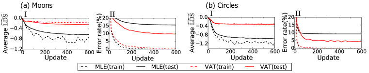
Figure 2 compares the learning process between the VAT and the MLE. Panels (a.I) and (b.I) show the transitions of the average , while panels (a.II) and (b.II) show the transitions of the error rate, on both training and test set. The average is nearly zero at the beginning, because the models are initially close to uniform distribution around each inputs. The average then decreases slowly for the VAT, and falls rapidly for the MLE. Although the training error eventually drops to zero for both methods, the final test error of the VAT is significantly lower than that of the MLE. This difference suggests that a high sustained value of is beneficial in alleviating the overfitting and in decreasing the test error.

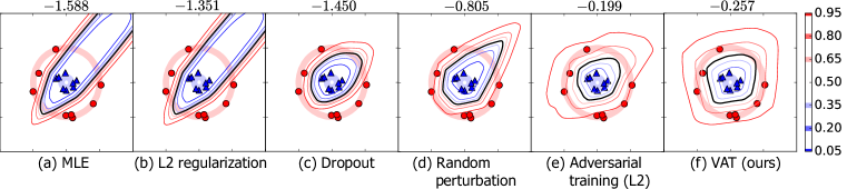
Figures 3 and 4 show the contour plot of the model distributions for the binary classification problems of ‘Moons’ and ‘Circles’ trained with the best set of hyper parameters. The value above each panel correspond to average value. We see from the figures that NN without regularization (MLE) and NN with regularization are drawing decisively wrong decision boundary. The decision boundary drawn by dropout for ‘Circles’ is convincing, but the dropout’s decision boundary for ‘Moons’ does not coincide with our intention. The opposite can be said for the random perturbation training. Only adversarial training and VAT are consistently yielding the intended decision boundaries for both datasets. VAT is drawing appropriate decision boundary by imposing local smoothness regularization around each data point. This does not mean, however, that the large value of LDS immediately implies good decision boundary. By its very definition, tends to disfavor abrupt change of the likelihood around training datapoint. Large value of therefore forces large relative margin around the decision boundary. One can achieve large value of with regularization, dropout and random perturbation training with appropriate choice of hyperparameters by smoothing the model distribution globally. This, indeed, comes at the cost of accuracy, however.
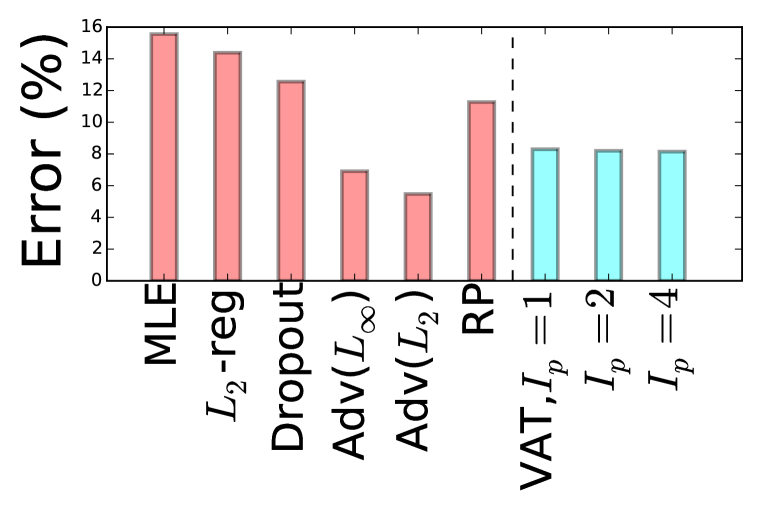

Figure 5 summarizes the average test errors of six regularization methods with the best set of hyperparameters. Adversarial training and VAT achieved much lower test errors than the other regularization methods. Surprisingly, the performance of the VAT did not change much with the value of . We see that suffices for our dataset.
3.2 Supervised learning for the classification of the MNIST dataset
Next, we tested the performance of our regularization method on the MNIST dataset, which consists of pixel images of handwritten digits and their corresponding labels. The input dimension is therefore and each label is one of the numerals from to . We split the original training samples into training samples and validation samples, and used the latter of which to tune the hyperparameters. We applied our methods to the training of 2 types of NNs with different numbers of layers, 2 and 4. As for the number of hidden units, we used and respectively. The ReLU activation function and batch normalization technique Ioffe & Szegedy (2015) were used for all the NNs. The detailed settings of the experiments are described in Appendix A.2.
For each regularization method, we used the set of hyperparameters that achieved the best performance on the validation data to train the NN on all training samples. We applied the trained networks to the test set and recorded their test errors. We repeated this procedure 10 times with different seeds for the weight initialization, and reported the average test error values.
Table 1 summarizes the test error obtained by our regularization method (VAT) and the other regularization methods. VAT performed better than all the contemporary methods except Ladder network, which is highly advanced generative model based method.
| Method | Test error (%) |
|---|---|
| SVM (gaussian kernel) | 1.40 |
| Gaussian dropout Srivastava et al. (2014) | 0.95 |
| Maxout Networks Goodfellow et al. (2013) | 0.94 |
| MTC Rifai et al. (2011) | 0.81 |
| DBM Srivastava et al. (2014) | 0.79 |
| Adversarial training Goodfellow et al. (2015) | 0.782 |
| Ladder network Rasmus et al. (2015) | 0.570.02 |
| Plain NN (MLE) | 1.11 |
| Random perturbation training | 0.843 |
| Adversarial training (with norm constraint) | 0.788 |
| Adversarial training (with norm constraint) | 0.708 |
| VAT (ours) | 0.637 |
3.3 Semi-supervised learning for the classification of the benchmark datasets
Recall that our definition of LDS (Eq.(3)) at any point is independent of the label information . This in particular means that we can apply the VAT to semi-supervised learning tasks. We would like to emphasize that this is a property not enjoyed by adversarial training and dropout. We applied VAT to semi-supervised learning tasks in the permutation invariant setting for three datasets: MNIST, SVHN, and NORB. In this section we describe the detail of our setup for the semi-supervised learning of the MNIST dataset, and leave the further details of the experiments in the Appendix A.3 and A.4.
We experimented with four sizes of labeled training samples and observed the effect of on the test error. We used the validation set of fixed size , and used all the training samples excluding the validation set and the labeled to train the NNs. That is, when , the unlabeled training set had the size of . For each choice of the hyperparameters, we repeated the experiment 10 times with different set. As for the architecture of NNs, we used ReLU based NNs with two hidden layers with the number of hidden units . Batch normalization was implemented as well.
Table 2(a) summarizes the results for the permutation invariant MNIST task. All the methods other than SVM and plain NN (MLE) are semi-supervised learning methods. For the MNIST dataset, VAT outperformed all the contemporary methods other than Ladder network Rasmus et al. (2015), which is current state of the art.
Table 2(b) and Table 2(c) summarizes the the results for SVHN and NORB respectively. Our method strongly outperforms the current state of the art semi-supervised learning method applied to these datasets.
| Method | Test error(%) | ||||
|---|---|---|---|---|---|
| SVM Weston et al. (2012) | 23.44 | 8.85 | 7.77 | 4.21 | |
| TSVM Weston et al. (2012) | 16.81 | 6.16 | 5.38 | 3.45 | |
| EmbedNN Weston et al. (2012) | 16.9 | 5.97 | 5.73 | 3.59 | |
| MTC Rifai et al. (2011) | 12.0 | 5.13 | 3.64 | 2.57 | |
| PEA Bachman et al. (2014) | 10.79 | 2.44 | 2.23 | 1.91 | |
| PEA Bachman et al. (2014) | 5.21 | 2.87 | 2.64 | 2.30 | |
| DG Kingma et al. (2014) | 3.33 | 2.59 | 2.40 | 2.18 | |
| Ladder network Rasmus et al. (2015) | 1.06 | 0.84 | |||
| Plain NN (MLE) | 21.98 | 9.16 | 7.25 | 4.32 | |
| VAT (ours) | 2.33 | 1.39 | 1.36 | 1.25 | |
4 Discussion and Related Works
Our VAT was motivated by the adversarial training Goodfellow et al. (2015). Adversarial training and VAT are similar in that they both use the local input-output relationship to smooth the model distribution in the corresponding neighborhood. In contrast, regularization does not use the local input-output relationship, and cannot introduce local smoothness to the model distribution. Increasing of the regularization constant in regularization can only intensify the global smoothing of the distribution, which results in higher training and generalization error. The adversarial training aims to train the model while keeping the average of the following value high:
| (13) |
This makes the likelihood evaluated at the -th labeled data point robust against perturbation applied to the input in its adversarial direction.
PEA Bachman et al. (2014), on the other hand, used the model’s sensitivity to random perturbation on input and hidden layers in their construction of the regularization function. PEA is similar to the random perturbation training of our experiment in that it aims to make the model distribution robust against random perturbation. Our VAT, however, outperforms PEA and random perturbation training. This fact is particularly indicative of the importance of the role of the hessian in VAT (Eq.(5)). Because PEA and random perturbation training attempts to smooth the distribution into any arbitrary direction at every step of the update, it tends to make the variance of the loss function large in unnecessary dimensions. On the other hand, VAT always projects the perturbation in the principal direction of , which is literally the principal direction into which the distribution is sensitive.
Deep contractive network by Gu and Rigazio Gu & Rigazio (2015) takes still another approach to smooth the model distribution. Gu et al. introduced a penalty term based on the Frobenius norm of the Jacobian of the neural network’s output with respect to . Instead of computing the computationally expensive full Jacobian, they approximated the Jabobian by the sum of the Frobenius norm of the Jacobian over every adjacent pairs of hidden layers. The deep contractive network was, however, unable to significantly decrease the test error.
Ladder network Rasmus et al. (2015) is a method that uses layer-wise denoising autoencoder. Their method is currently the best method in both supervised and semi-supervised learning for permutation invariant MNIST task. Ladder network seems to be conducting a variation of manifold learning that extracts the knowledge of the local distribution of the inputs. Still another classic way to include the information about the the input distribution is to use local smoothing of the data like Vicinal Risk Minimization (VRM) Chapelle et al. (2001). VAT, on the other hand, only uses the property of the conditional distribution , giving no consideration to the the generative process nor to the full joint distribution In this aspect, VAT can be complementary to the methods that explicitly model the input distribution. We might be able to improve VAT further by introducing the notion of manifold learning into its framework.
5 Conclusion
Our experiments based on the synthetic datasets and the three real world dataset, MNIST, SVHN and NORB indicate that the VAT is an effective method for both supervised and semi-supervised learning. For the MNIST dataset, VAT outperformed all contemporary methods other than Ladder network, which is the current state of the art. VAT also outperformed current state of the art semi-supervised learning method for SVHN and NORB as well. We would also like to emphasize the simplicity of the method. With our approximation of LDS, VAT can be computed with relatively small computational cost. Also, models that relies heavily on generative models are dependent on many hyperparameters. VAT, on the other hand, has only two hyperparamaters, and . In fact, our experiments worked sufficiently well with the optimization of one hyperparameter while fixing .
References
- Akaike (1998) Akaike, Hirotugu. Information theory and an extension of the maximum likelihood principle. In Selected Papers of Hirotugu Akaike, pp. 199–213. Springer, 1998.
- Bachman et al. (2014) Bachman, Phil, Alsharif, Ouais, and Precup, Doina. Learning with pseudo-ensembles. In Advances in Neural Information Processing Systems, 2014.
- Bastien et al. (2012) Bastien, Frédéric, Lamblin, Pascal, Pascanu, Razvan, Bergstra, James, Goodfellow, Ian J., Bergeron, Arnaud, Bouchard, Nicolas, and Bengio, Yoshua. Theano: new features and speed improvements. Workshop on Deep Learning and Unsupervised Feature Learning at Neural Information Processing Systems, 2012.
- Bengio (2009) Bengio, Yoshua. Learning deep architectures for ai. Foundations and trends® in Machine Learning, 2(1):1–127, 2009.
- Bergstra et al. (2010) Bergstra, James, Breuleux, Olivier, Bastien, Frédéric, Lamblin, Pascal, Pascanu, Razvan, Desjardins, Guillaume, Turian, Joseph, Warde-Farley, David, and Bengio, Yoshua. Theano: a CPU and GPU math expression compiler. In Proceedings of the Python for Scientific Computing Conference (SciPy), June 2010. Oral Presentation.
- Chapelle et al. (2001) Chapelle, Olivier, Weston, Jason, Bottou, Léon, and Vapnik, Vladimir. Vicinal risk minimization. In Advances in Neural Information Processing Systems, 2001.
- Coates et al. (2011) Coates, Adam, Ng, Andrew Y, and Lee, Honglak. An analysis of single-layer networks in unsupervised feature learning. In International Conference on Artificial Intelligence and Statistics, pp. 215–223, 2011.
- Friedman et al. (2001) Friedman, Jerome, Hastie, Trevor, and Tibshirani, Robert. The elements of statistical learning. Springer series in statistics Springer, Berlin, 2001.
- Glorot et al. (2011) Glorot, Xavier, Bordes, Antoine, and Bengio, Yoshua. Deep sparse rectifier neural networks. In International Conference on Artificial Intelligence and Statistics, pp. 315–323, 2011.
- Golub & Van der Vorst (2000) Golub, Gene H and Van der Vorst, Henk A. Eigenvalue computation in the 20th century. Journal of Computational and Applied Mathematics, 123(1):35–65, 2000.
- Goodfellow et al. (2013) Goodfellow, Ian J, Warde-Farley, David, Mirza, Mehdi, Courville, Aaron, and Bengio, Yoshua. Maxout networks. In International Conference on Machine Learning, 2013.
- Goodfellow et al. (2015) Goodfellow, Ian J, Shlens, Jonathon, and Szegedy, Christian. Explaining and harnessing adversarial examples. In International Conference on Learning Representation, 2015.
- Gu & Rigazio (2015) Gu, Shixiang and Rigazio, Luca. Towards deep neural network architectures robust to adversarial examples. In International Conference on Learning Representation, 2015.
- Ioffe & Szegedy (2015) Ioffe, Sergey and Szegedy, Christian. Batch normalization: Accelerating deep network training by reducing internal covariate shift. In International Conference on Machine Learning, 2015.
- Jarrett et al. (2009) Jarrett, Kevin, Kavukcuoglu, Koray, Ranzato, Marc’Aurelio, and LeCun, Yann. What is the best multi-stage architecture for object recognition? In Computer Vision, 2009 IEEE 12th International Conference on, pp. 2146–2153. IEEE, 2009.
- Jia et al. (2014) Jia, Yangqing, Shelhamer, Evan, Donahue, Jeff, Karayev, Sergey, Long, Jonathan, Girshick, Ross, Guadarrama, Sergio, and Darrell, Trevor. Caffe: Convolutional architecture for fast feature embedding. In Proceedings of the ACM International Conference on Multimedia, pp. 675–678. ACM, 2014.
- Kingma & Ba (2015) Kingma, Diederik and Ba, Jimmy. Adam: A method for stochastic optimization. In International Conference on Learning Representation, 2015.
- Kingma et al. (2014) Kingma, Diederik, Mohamed, Shakir, Rezende, Danilo Jimenez, and Welling, Max. Semi-supervised learning with deep generative models. In Advances in Neural Information Processing Systems, 2014.
- LeCun et al. (2015) LeCun, Yann, Bengio, Yoshua, and Hinton, Geoffrey. Deep learning. Nature, 521(7553):436–444, 2015.
- Nair & Hinton (2010) Nair, Vinod and Hinton, Geoffrey E. Rectified linear units improve restricted boltzmann machines. In International Conference on Machine Learning, 2010.
- Pearlmutter (1994) Pearlmutter, Barak A. Fast exact multiplication by the hessian. Neural computation, 6(1):147–160, 1994.
- Rasmus et al. (2015) Rasmus, Antti, Valpola, Harri, Honkala, Mikko, Berglund, Mathias, and Raiko, Tapani. Semi-supervised learning with ladder network. arXiv preprint arXiv:1507.02672, 2015.
- Rifai et al. (2011) Rifai, Salah, Dauphin, Yann N, Vincent, Pascal, Bengio, Yoshua, and Muller, Xavier. The manifold tangent classifier. In Advances in Neural Information Processing Systems, 2011.
- Srivastava et al. (2014) Srivastava, Nitish, Hinton, Geoffrey, Krizhevsky, Alex, Sutskever, Ilya, and Salakhutdinov, Ruslan. Dropout: A simple way to prevent neural networks from overfitting. The Journal of Machine Learning Research, 15(1):1929–1958, 2014.
- Tokui et al. (2015) Tokui, Seiya, Oono, Kenta, Hido, Shohei, and Clayton, Justin. Chainer: a next-generation open source framework for deep learning. In Workshop on Machine Learning Systems at Neural Information Processing Systems, 2015.
- Wahba (1990) Wahba, Grace. Spline models for observational data. Siam, 1990.
- Watanabe (2009) Watanabe, Sumio. Algebraic geometry and statistical learning theory. Cambridge University Press, 2009.
- Weston et al. (2012) Weston, Jason, Ratle, Frédéric, Mobahi, Hossein, and Collobert, Ronan. Deep learning via semi-supervised embedding. In Neural Networks: Tricks of the Trade, pp. 639–655. Springer, 2012.
Appendix A Appendix:Details of experimental settings
A.1 Supervised binary classification for synthetic datasets
We provide more details of experimental settings on synthetic datasets. We list the search space for the hyperparameters below:
-
•
regularization: regularization coefficient
-
•
Dropout (only for the input layer): dropout rate
-
•
Random perturbation training:
-
•
Adversarial training (with norm constraint):
-
•
Adversarial training (with norm constraint):
-
•
VAT:
All experiments with random perturbation training, adversarial training and VAT were conducted with . As for the training we used stochastic gradient descent (SGD) with a moment method. When is the objective function, the moment method augments the simple update in the SGD with a term dependent on the previous update :
| (14) |
In the expression above, stands for the strength of the momentum, and stands for the learning rate. In our experiment, we used , and exponentially decreasing with rate . As for the choice of , we used . We trained the NNs with 1,000 parameter updates.
A.2 Supervised classification for the MNIST dataset
We provide more details of experimental settings on supervised classification for the MNIST dataset. Following lists summarizes the ranges from which we searched for the best hyperparameters of each regularization method:
-
•
Random perturbation training:
-
•
Adversarial training (with norm constraint):
-
•
Adversarial training (with norm constraint):
-
•
VAT: ,
All experiments were conducted with . The training was conducted by mini-batch SGD based on ADAM Kingma & Ba (2015). We chose the mini-batch size of 100, and used the default values of Kingma & Ba (2015) for the tunable parameters of ADAM. We trained the NNs with 50,000 parameter updates. As for the base learning rate in validation, we selected the initial value of and adopted the schedule of exponential decay with rate per 500 updates. After the hyperparameter determination, we trained the NNs over 60,000 parameter updates. For the learning coefficient, we used the initial value of and adopted the schedule of exponential decay with rate per 600 updates.
A.3 Semi-supervised classification for the MNIST dataset
We provide more details of experimental settings on semi-supervised classification for the MNIST dataset. We searched for the best hyperparameter from in the case. Best was selected from for all other cases. All experiments were conducted with and . For the optimization method, we again used ADAM-based minibatch SGD with the same hyperparameter values as those in the supervised setting. We note that, in the computation of ADAM, the likelihood term can be computed from labeled data only. We therefore used two separate minibatches at each step: one minibatch of size 100 from labeled samples for the computation of the likelihood term, and another minibatch of size 250 from both labeled and unlabeled samples for computing the regularization term. We trained the NNs over 50,000 parameter updates. For the learning rate, we used the initial value of and adopted the schedule of exponential decay with rate per 500 updates.
A.4 Semi-supervised classification for the SVHN and NORB dataset
We provide the details of the numerical experiment we conducted for the SVHN and NORB dataset.
The SVHN dataset consists of pixel RGB images of housing numbers and their corresponding labels (0-9), and the number of training samples and test samples within the dataset are 73,257 and 26,032,
respectively. To simplify the experiment, we down sampled the images from to
. We vectorized each image to 768 dimensional vector, and applied whitening Coates et al. (2011) to the dataset. We reserved 1000 dataset for validation. From the rest, we used 1000 dataset as labeled dataset in semi-supervised training. We repeated the experiment 10 times with different choice of labeled dataset and validation dataset.
The NORB dataset consists of pixel gray images of 50 different objects and their corresponding labels (cars, trucks, planes, animals, humans). The number of training samples and test samples constituting the dataset are 24,300. We downsampled the images from to . We vectorized each image to 2048 dimensional vector and applied whitening. We reserved 1000 dataset for validation. From the rest, we used 1000 dataset as labeled dataset in semi-supervised training. We repeated the experiment 10 times with different choice of labeled dataset and validation dataset.
For both SVHN and NORB, we used neural network with the number of hidden nodes given by . In our setup, these two dataset preferred deeper network than the network we used for the MNIST dataset. We used ReLU for the activation function. As for the hyperparameters , we conducted grid search over the range , and we used . For power iteration, we used .
We used ADAM based minibach SGD with the same hyperparameter values as the MNIST. We chose minibatch size of 100. Thus one epoch for SVHN completes with rounds of minibatches. For the learning rate, we used the initial value of with exponential decay of rate per epoch. We trained NNs with 100 epochs.