Pulse design without rotating wave approximation

Abstract

We design realizable time-dependent semiclassical pulses to invert the population of a two-level system faster than adiabatically when the rotating-wave approximation cannot be applied. Different approaches, based on the counterdiabatic method or on invariants, may lead to singularities in the pulse functions. Ways to avoid or cancel the singularities are put forward when the pulse spans few oscillations. For many oscillations an alternative numerical minimization method is proposed and demonstrated.

I Introduction

Controlling accurately the internal states of quantum two-level systems, realized by real or artificial atoms, as in crystal defects, quantum dots, or superconducting qubits, is a fundamental task in nuclear magnetic resonance, metrology or to develop new quantum technologies sta ; sun ; lin ; tseng ; deschamps ; collin ; torosov ; sillanpaa ; leek . Pulse engineering is the art and science of designing realizable control fields to perform specific operations. We assume here that the field is intense enough to be treated semiclassically. The task amounts to solving an “inverse problem”, as the aim is to determine a realizable Hamiltonian that drives the system to specific states at a given final time, e.g., the ones that would be reached in an ideal adiabatic driving ChenPRA . The design and implementation of the pulse are easier for adiabatic dynamics, as the final atomic state is quite insensitive to smooth deviations from the ideal pulse, but for faster-than-adiabatic processes, the design and its implementation become more demanding. In addition, when the rotating-wave approximation (RWA) Allen fails for strong drivings, the inversion process becomes more involved. However, this regime is key to achieve fast control of two-level systems, e.g., in nitrogen-vacancy centers fuchs ; london ; childress .

In this paper we focus on speeding up “rapid adiabatic passage” (RAP) population inversion processes in two-level systems ChenPRA ; ChenPRL ; zhang , beyond the RWA. Without the RWA, a consistency condition between the diagonal and the non-diagonal elements of the interaction-picture Hamiltonian, which involves the phase $\varphi(t)$ of the field and its derivative with respect to time, $\dot{\varphi}(t)$, must be satisfied. We shall first apply the counterdiabatic (CD) method Rice03 ; Rice05 ; Rice08 ; Berry09 ; ChenPRL . In this method, a reference Hamiltonian, i.e., the Hamiltonian for the two-level system without the RWA in the interaction picture, $H(t)$, is complemented (or even substituted) by a CD Hamiltonian, $H_{1}(t)$, so that the system follows exactly the adiabatic dynamics of $H(t)$. In the dynamics driven by $H(t)+H_{1}(t)$, the CD term suppresses transitions in the instantaneous eigenbasis of $H$, but allows for transitions in the instantaneous eigenbasis of $H+H_{1}$. This Hamiltonian, however, does not necessarily satisfy the consistency condition mentioned above, unless an appropriate rearrangement of terms is performed, and a new unitary transformation between interaction and Schrödinger pictures, different from the one for $H$, is implemented prl . In section II we show that the consistent field implies in general singularities in the Rabi frequency, but the field itself is not singular.

We use as well invariants of motion LR . Designing the invariant is equivalent to imposing the desired dynamics. This is easy within the RWA by setting the time dependence of independent auxiliary variables corresponding to polar, $\theta(t)$, and azimuthal angles, $\beta(t)$, that characterize the invariant eigenstates on the Bloch sphere ChenPRA . From these angles the time dependences of the Hamiltonian components, the Rabi frequency $\Omega_{R}(t)$ and the detuning $\Delta(t)$, and thus the physical fields may be deduced ChenPRA . By contrast, without applying the RWA, a naive independent design leads to singularities in the field. In section III we show two different ways to avoid this problem. When the pulse duration spans only a few field oscillations the angles $\theta$ and $\beta$ may be set to cancel all singularities and produce a smooth, finite-intensity pulse. Instead, if many field oscillations occur, a numerical minimization method to find optimal parameters in a predetermined pulse form may be used to invert the population.

We shall set first the basic concepts and notation. Assuming a semiclassical interaction between the electric field, $E(t)=E_{0}(t)\cos[\varphi(t)]$, and the two-level atom, the Hamiltonian of the atom in the Schrödinger picture, in the electric dipole approximation, is, see e.g. Alvaro ,

$$H_{s}(t) = \frac{\hbar}{2}\Big{\{}\omega_{0}(t)(|e\rangle\langle e|-|g\rangle\langle g|)$$ (1)

$$+ \Omega_{R}(t)[(|e\rangle\langle g|+|g\rangle\langle e|)(e^{i\varphi(t)}+e^{-i\varphi(t)})]\Big{\}},$$

in the bare basis of the atom $|g\rangle=(\tiny{\begin{array}[]{c}1\\ 0\end{array}})$, $|e\rangle=(\tiny{\begin{array}[]{c}0\\ 1\end{array}})$, where $\omega_{0}(t)/(2\pi)$ is the transition frequency of the atom, which may in general depend on time, controlled, e.g., by Stark shifts; $\Omega_{R}(t)$ is the Rabi frequency, assumed real (without loss of generality for transitions without change in the magnetic number, see Allen ); and $\varphi(t)$ is the time dependent phase of the electric field of the pulse, where $\dot{\varphi}(t)/(2\pi)$ is the instantaneous field frequency. The “exact” Hamiltonian, i.e., without applying the RWA, in a field-adapted interaction picture is given by Alvaro

$$H(t)=U^{\dagger}_{\varphi}(H_{s}-H_{\varphi})U_{\varphi},$$ (2)

where

$$H_{\varphi}(t)=\frac{\hbar\dot{\varphi}}{2}(|e\rangle\langle e|-|g\rangle\langle g|)$$ (3)

and

$$U_{\varphi}(t) = e^{-i\int_{0}^{t}{H_{\varphi}(t^{\prime})dt^{\prime}}/\hbar}$$ (4)

$$= e^{-i\varphi(t)/2}|e\rangle\langle e|+e^{i\varphi(t)/2}|g\rangle\langle g|$$

is the unitary operator of the transformation. Thus,

$$H(t)=\frac{\hbar}{2}\left(\begin{array}[]{cc}-\Delta&\Omega\\ \Omega^{*}&\Delta\end{array}\right),$$ (7)

with

$$\Omega(t)=\Omega_{R}(t)[1+e^{-2i\varphi(t)}],$$ (8)

and detuning

$$\Delta(t)=\omega_{0}(t)-\dot{\varphi}(t).$$ (9)

The eigenenergies of $H$ are $E_{\pm}(t)=\pm\hbar\varepsilon_{0}(t)/2$, with $\varepsilon_{0}(t)=\sqrt{\Delta(t)^{2}+|\Omega(t)|^{2}}$, and the (time dependent) eigenstates, $|{\pm}\rangle\equiv|{\pm}(t)\rangle$, are

$$|\pm\rangle = \left[\frac{-(\Delta\mp\varepsilon_{0})}{\Omega^{*}}|g\rangle+|e\rangle\right]\frac{1}{\sqrt{1+\frac{(\Delta\mp\varepsilon_{0})^{2}}{|\Omega|^{2}}}},$$ (10)

which satisfy $H(t)|{\pm}(t)\rangle=E_{\pm}(t)|{\pm}(t)\rangle$.

The exact two-level system Hamiltonian in the interaction picture entails $\dot{\varphi}(t)$ in the detuning, i.e., in the diagonal elements, see Eq. (9), and its integral, $\varphi(t)$, in the non-diagonal elements, see Eq. (8). By “consistency condition” we mean that the elements of a physically allowed interaction picture Hamiltonian must comply with the structure set in Eqs. (8) and (9). In particular, this structure must be satisfied when designing pulses to carry out faster-than-adiabatic inversion processes, as we shall see in sections II and III. Suppose for example that the functions $\Omega_{R}(t)$ and $\omega_{0}(t)$ are given. Then, not any Hamiltonian is allowed (consistent) since the diagonal and non-diagonal parts must depend on $\varphi(t)$ and its derivative consistently.

II The counterdiabatic method

The counterdiabatic approach adds a counterdiabatic or “CD” term to some reference Hamiltonian to make the exact dynamics adiabatic with respect to the reference Hamiltonian Rice03 ; Rice05 ; Rice08 ; Berry09 ; ChenPRL . The formal construction of the CD term is explained in the original references Rice03 ; Rice05 ; Rice08 ; Berry09 ; ChenPRL ; ChenPRA . We shall apply the counterdiabatic method to speed up an adiabatic population inversion process for a two-level systems beyond the RWA, where the (reference) Hamiltonian of the system is given by Eq. (7), or in diagonal form as $H(t)=\sum_{n}|n(t)\rangle E_{n}(t)\langle n(t)|$, where $|n(t)\rangle=|\pm(t)\rangle$. The inversion is from $|\Psi(0)\rangle=|g\rangle$ to $|\Psi(t_{f})\rangle=|e\rangle$, up to a phase factor, where $t=0$ and $t=t_{f}$ are the initial and final times of the process, and $|\Psi(t)\rangle$ is the general state of the system. We consider a constant field (angular) frequency, $\dot{\varphi}(t)=\omega_{L}$, so that $\varphi(t)=\omega_{L}t$, and a time dependent transition frequency, $\omega_{0}(t)/(2\pi)$, that will determine the detuning. Then, from Eqs. (8) and (9),

$$\Omega(t) = \Omega_{R}(1+e^{-2i\omega_{L}t}),$$ (11)

$$\Delta(t) = \omega_{0}(t)-\omega_{L}.$$ (12)

The CD term is in general given by, see e.g. Berry09 ,

$$H_{1}(t) = i\hbar\sum_{n}(|\partial_{t}{n}\rangle\langle n|-\langle n|\partial_{t}{n}\rangle|n\rangle\langle n|)$$

$$= i\hbar\sum_{m\neq n}\sum\frac{|m\rangle\langle m|\partial_{t}H|n\rangle\langle n|}{E_{n}-E_{m}}.$$

For the exact two-level system, using Eq. (10), $H_{1}$ is given by ChenWei

$$H_{1}(t) = \frac{i\hbar}{2C_{1}}\left(\begin{array}[]{cc}-B_{1}/2&A_{1}\\ -A_{1}^{*}&B_{1}/2\end{array}\right),$$ (15)

where $A_{1}(t)=\dot{\Omega}\Delta-\dot{\Delta}\Omega$, $B_{1}(t)=\dot{\Omega}^{*}\Omega-\dot{\Omega}\Omega^{*}$ is purely imaginary, and $C_{1}(t)=\Delta^{2}+|\Omega|^{2}$. Thus, the total Hamiltonian provided by the CD method is

$$H+H_{1} = \frac{\hbar}{2}\left(\begin{array}[]{cc}-\tilde{\Delta}&\tilde{\Omega}\\ \tilde{\Omega}^{*}&\tilde{\Delta}\end{array}\right),$$ (18)

where

$$\tilde{\Omega} = \Omega+iA_{1}/C_{1},$$ (19)

$$\tilde{\Delta} = \Delta+iB_{1}/2C_{1}.$$ (20)

From Eq. (12), the detuning of the total Hamiltonian, given by Eq. (20), becomes

$$\tilde{\Delta}=(\omega_{0}+iB_{1}/2C_{1})-\omega_{L}.$$ (21)

The term $\omega_{0}+iB_{1}/2C_{1}$ may be interpreted as a new time-dependent transition (angular) frequency, and $\omega_{L}/(2\pi)$ is, as in the reference Hamiltonian, the constant field frequency. Then, the non-diagonal element $\tilde{\Omega}$, given by Eq. (19), should be expressed as $\tilde{\Omega}=\tilde{\Omega}_{R}(1+e^{-2i\omega_{L}t})$, compare with Eq. (11), in order to satisfy the consistency condition, where $\tilde{\Omega}_{R}\equiv\tilde{\Omega}_{R}(t)$ is a new Rabi frequency corresponding to the pulse associated with $H+H_{1}$.

To see whether $H+H_{1}$ is indeed consistent we first rewrite the complex $\tilde{\Omega}$ in Eq. (19) in a convenient form,

$$\tilde{\Omega} = \tilde{\Omega}_{R}(1+e^{-2i\tilde{\varphi}})$$ (22)

$$= 2\tilde{\Omega}_{R}\cos{\tilde{\varphi}}e^{-i\tilde{\varphi}},$$ (23)

where $\tilde{\Omega}_{R}$ and $\tilde{\varphi}\equiv\tilde{\varphi}(t)$ are real. $\tilde{\varphi}$ is given by

$$\tilde{\varphi}=-\arg(\tilde{\Omega})+2\pi n,$$ (24)

where n is an integer chosen to make $\tilde{\varphi}$ continuous. Once $\tilde{\varphi}$ is determined, taking into account Eq. (19), $\tilde{\Omega}_{R}$ is calculated from Eqs. (22) or (23). However, the consistency condition is generally not satisfied, i.e., $\tilde{\varphi}\neq\varphi=\omega_{L}t$. For the Allen-Eberly protocol Allen ,

$$\Omega_{R}(t) = \Omega_{M}\sinh{\left[\frac{\pi(t-t_{f}/2)}{2t_{0}}\right]},$$

$$\Delta(t) = \frac{2\delta^{2}t_{0}}{\pi}\tanh{\left[\frac{\pi(t-t_{f}/2)}{2t_{0}}\right]},$$ (25)

and parameters $\Omega_{M}=2\pi\times 3$ MHz, $\delta=2\pi\times 200$ MHz, $t_{0}=0.05$ ns, $\omega_{L}=2\pi\times 10$ GHz, and $t_{f}=0.4$ ns, Fig. 1 (a) shows that $\varphi(t)=\omega_{L}t$ and $\tilde{\varphi}(t)$ do not coincide. These parameters are chosen so that $H(t)$ does not invert the populations of the bare basis, $P_{g}(t)=|\langle g|\Psi(t)\rangle|^{2}$ and $P_{e}(t)=|\langle e|\Psi(t)\rangle|^{2}$. Fig. 1 (b) shows that the Hamiltonian $H+H_{1}$ does invert the population. The CD term works formally, but the Hamiltonian $H+H_{1}$ does not correspond to a field with frequency $\omega_{L}/(2\pi)$. If we apply the same transformation that relates the Schrödinger picture Hamiltonian $H_{s}$ and the interaction-picture Hamiltonian $H$,

$$U_{\varphi}(t)=e^{-i\omega_{L}t/2}|e\rangle\langle e|+e^{i\omega_{L}t/2}|g\rangle\langle g|,$$ (26)

for $\varphi=\omega_{L}t$, following Eq. (2), the Schrödinger picture Hamiltonian corresponding to $H+H_{1}$ does not take the form of Eq. (1) with modified functions for the transition and Rabi frequencies. This procedure is schematized in Fig. 2 by the boxes around $S,\,I$, and $S^{\prime},\,I^{\prime}$, where $S$ represents the initial Schrödinger picture driven by $H_{s}$ and $I$ the interaction picture driven by $H$ with $U_{\varphi}$, given by Eq. (26), the unitary operator that generates the transformation. $I^{\prime}$ represents the interaction picture with the addition of an extra term, $H+H_{1}$, and $S^{\prime}$ the corresponding Schrödinger picture mediated again by Eq. (26).

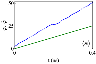
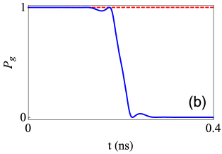
Figure 1: (Color online) (a) $\varphi(t)=\omega_{L}t$ (green solid line) and $\tilde{\varphi}(t)$ given by Eq. (24) (blue short-dashed line), (b) $P_{g}$ driven by $H$ (red dashed line) and by $H+H_{1}$ (blue solid line), and (c) $\tilde{\omega}_{0}(t)=\tilde{\Delta}+\dot{\tilde{\varphi}}$ divided by $2\pi$, for the Allen-Eberly protocol and parameters: $\Omega_{M}=2\pi\times 3$ MHz, $\delta=2\pi\times 200$ MHz, $t_{0}=0.05$ ns, $\omega_{L}=2\pi\times 10$ GHz, and $t_{f}=0.4$ ns.

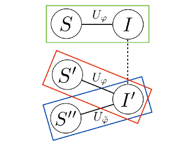
Figure 2: (Color online) Schematic relation between different Schrödinger and interaction picture dynamical equations. Each node may represent the dynamical equations, and also the Hamiltonian or the states. The rectangular boxes enclose nodes that represent the same underlying physics. The solid lines represent unitary relations for the linked states and the dashed line represents a non-unitary addition of a term to the Hamiltonian.

We might as well assume that $H_{1}$ is a Hamiltonian corresponding to an independent (second) pulse complementing the pulse for $H$. This, however, leads to the same result as interpreting $H+H_{1}$ as a single pulse, since $H$ is negligible versus $H_{1}$, i.e., $|\Omega|\ll|iA_{1}/C_{1}|$ and $\Delta\ll iB_{1}/(2C_{1})$, for the given parameters. The consistency condition is again not satisfied.

To enforce the consistency condition between the diagonal and non-diagonal elements in Eq. (18) we may rewrite $\tilde{\Delta}$, see Eq. (21), with the required structure, i.e., $\tilde{\Delta}=\tilde{\omega}_{0}(t)-\dot{\tilde{\varphi}}$, where $\tilde{\omega}_{0}(t)/(2\pi)$ is a new time-dependent transition frequency of the atom. Equating this expression to Eq. (21) gives

$$\tilde{\omega}_{0}(t)=\omega_{0}-\omega_{L}+iB_{1}/2C_{1}+\dot{\tilde{\varphi}},$$

which is depicted in Fig. 1 (c) with $\omega_{0}(t)$ obtained from Eq. (12) and $\Delta$ given by Eq. (25). The unitary transformation $U_{\tilde{\varphi}}$, where $\varphi$ is substituted by $\tilde{\varphi}$ in Eqs. (3) and (4), leads to a different Schrödinger picture $S^{\prime\prime}$ prl , see Fig. 2. The Hamiltonian in the Schrödinger picture $S^{\prime\prime}$ is

$$H_{S^{\prime\prime}}(t) = \frac{\hbar}{2}\left(\begin{array}[]{cc}-\tilde{\omega}_{0}&2\tilde{\Omega}_{R}\cos\tilde{\varphi}\\ 2\tilde{\Omega}_{R}\cos\tilde{\varphi}&\tilde{\omega}_{0}\end{array}\right).$$ (29)

This procedure solves the consistency condition, but the new Rabi frequency, given by Eqs. (22) or (23), is singular at the zeros of $\cos{\tilde{\varphi}}$. However, the field, proportional to $\tilde{\Omega}_{R}\cos{\tilde{\varphi}}$, is well behaved, see Fig. 3.

Figure 3: $2\tilde{\Omega}_{R}\cos{\tilde{\varphi}}/(2\pi)$ for parameters as in the caption of Fig. 1.

In the following section we work out a different approach based on invariants of the motion.

III Invariant-based inverse engineering

Associated with $H(t)$ there are hermitian dynamical invariants, $I(t)$, satisfying the invariance condition LR ,

$$\frac{\partial{I}}{\partial{t}}+\frac{1}{i\hbar}[I,H]=0,$$ (30)

that may be parametrized as ChenPRA ; inva ; inva1

$$I(t)=\frac{\hbar I_{0}}{2}\left(\begin{array}[]{cc}\cos{\theta}&\sin{\theta}e^{-i\beta}\\ \sin{\theta}e^{i\beta}&-\cos{\theta}\end{array}\right),$$ (33)

where $I_{0}$ is an arbitrary constant angular frequency to keep $I(t)$ with dimensions of energy, and $\theta\equiv\theta(t)$ and $\beta\equiv\beta(t)$ are the polar and azimuthal angles in the Bloch sphere, respectively. The eigenvalue equation for $I(t)$ is $I(t)|\phi_{\pm}^{I}(t)\rangle=\lambda_{\pm}|\phi_{\pm}^{I}(t)\rangle$, where the eigenvalues are $\lambda_{\pm}=\pm\hbar I_{0}/2$ and, consistently with orthogonality and normalization, we can choose the basis of eigenstates

$$|\phi_{+}^{I}(t)\rangle=\Bigg{(}\!\begin{array}[]{c}\cos{\frac{\theta}{2}}e^{-i\frac{\beta}{2}}\\ \sin{\frac{\theta}{2}}e^{i\frac{\beta}{2}}\end{array}\!\Bigg{)},\,|\phi_{-}^{I}(t)\rangle=\Bigg{(}\!\begin{array}[]{c}\sin{\frac{\theta}{2}}e^{-i\frac{\beta}{2}}\\ -\cos{\frac{\theta}{2}}e^{i\frac{\beta}{2}}\end{array}\!\Bigg{)}.$$ (34)

The solution of the time-dependent Schrödinger equation, $i\hbar\partial_{t}|\Psi(t)\rangle=H(t)|\Psi(t)\rangle$, can be expressed as LR

$$|\Psi(t)\rangle=c_{+}e^{i\gamma_{+}(t)}|\phi_{+}^{I}(t)\rangle+c_{-}e^{i\gamma_{-}(t)}|\phi_{-}^{I}(t)\rangle,$$

up to a global phase factor, where the $c_{\pm}$ are time-independent coefficients and the $\gamma_{\pm}(t)$ are the Lewis-Riesenfeld phases,

$$\gamma_{\pm}(t)=\frac{1}{\hbar}\int_{0}^{t}\Big{\langle}\phi_{\pm}^{I}(t^{\prime})\Big{|}i\hbar\frac{\partial}{\partial t^{\prime}}-H(t^{\prime})\Big{|}\phi_{\pm}^{I}(t^{\prime})\Big{\rangle}dt^{\prime}.$$

The Lewis-Riesenfeld phase becomes a global phase if the dynamics is carried out by one eigenstate of the invariant only. This will be the case in the inversions discussed here and leads to an important simplification: $\gamma_{\pm}(t)$ can be ignored to engineer the Hamiltonian.

From the invariance condition (30), with $I$ given by Eq. (33) and $H$ given by Eq. (7), we find

$$\dot{\theta} = -2\Omega_{R}\cos\varphi\sin(\beta-\varphi),$$

$$\dot{\beta} = -\Delta-2\Omega_{R}\cot{\theta}\cos{\varphi}\cos(\beta-\varphi).$$ (35)

The first equation bounds $\dot{\theta}$ between $-2\Omega_{R}$ and $2\Omega_{R}$. These equations are much simplified when the RWA may be applied ChenPRA . The two-level system Hamiltonian under the RWA is, see for example ChenPRA ,

$$H_{RWA}(t)=\frac{\hbar}{2}\left(\begin{array}[]{cc}-\Delta&\Omega_{R}\\ \Omega_{R}&\Delta\end{array}\right),$$ (38)

where $\varphi(t)$ is absent in the non-diagonal elements of $H_{RWA}(t)$, compare with $H(t)$ in Eq. (7). Now the spherical angles satisfy ChenPRA ; inva ; inva1

$$RWA\left\{\begin{array}[]{lll}\dot{\theta}&=&-\Omega_{R}\sin{\beta},\\ \dot{\beta}&=&-\Delta-\Omega_{R}\cot{\theta}\cos{\beta}.\end{array}\right.$$ (41)

The “direct problem” is to solve the systems of differential equations (35) or (41) for $\theta$ and $\beta$ when $\Omega_{R}$ and $\Delta$ are given, once we fix $\omega_{0}$ or $\varphi$ for the system (35), see also Eq. (9). Instead, in the “inverse problem” we have in principle to construct the functions $\Omega_{R}$ and $\Delta$ from $\theta$ and $\beta$. When the RWA holds, from the system (41), the inversion reduces to simple expressions for $\Omega_{R}$ and $\Delta$ ChenPRA ,

$$RWA\left\{\begin{array}[]{lll}\Omega_{R}&=&-\dot{\theta}/\sin\beta,\\ \Delta&=&-\dot{\beta}+\dot{\theta}\cot\theta\cot\beta.\end{array}\right.$$ (44)

Without the RWA, from the system (35), taking into account Eq. (9), we get

$$\Omega_{R} = -\frac{\dot{\theta}}{2\cos\varphi\sin{\alpha}},$$ (45)

$$\dot{\alpha} = -\omega_{0}+{\dot{\theta}}{\cot{\theta}}\cot{\alpha},$$ (46)

where $\alpha(t)=\beta(t)-\varphi(t)$ is introduced to simplify the expressions. If the inversion strategy is to consider $\omega_{0}(t)$ as given, which in particular could be constant, and $\theta(t)$ is designed, the differential equation for $\alpha(t)$, see Eq. (46), is problematic, as an arbitrary choice of $\theta(t)$ and $\omega_{0}(t)$ will typically lead to singularities on the right hand side, and $\alpha(t)$ will, in general, introduce singularities in $\Omega_{R}(t)$. Eq. (45) makes clear that a finite, smooth $\Omega_{R}$ and a phase $\varphi$ increasing along many field cycles, require many zeros of $\dot{\theta}$ to compensate for zeros in the denominator. A naive choice for $\theta$ is thus doomed to fail. A different approach is needed. It is useful to rewrite Eq. (46), taking into account Eq. (9), as

$$\Delta=-(\dot{\varphi}+\dot{\alpha})+{\dot{\theta}}\,{\cot{\theta}}\cot{\alpha}.$$ (47)

Even if $\theta$ and $\alpha$ avoid the singularities for a given $\varphi$ in Eq. (47), the required consistency between Eqs. (9) and (47) (they must be equal) will in general fail if $\omega_{0}(t)$ is also given. Thus, the proposed strategy is to fix first $\varphi(t)$, then design $\theta(t)$ to avoid the zeros of $\cos\varphi$ in Eq. (45), and from there design $\alpha(t)$ to compensate singularities of $\cot\theta$ in Eq. (47). This produces a smooth $\Omega_{R}$ given by Eq. (45), and $\Delta$ follows from Eq. (47). Finally, $\omega_{0}(t)$ is deduced consistently from Eq. (9).

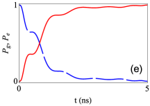
Figure 4: (Color online) Interpolated functions (a) $\theta$ and (b) $\alpha$ for a population inversion process with parameters $\omega_{L}=2\pi\times 500$ MHz and $t_{f}=5$ ns. (c) and (d) show the corresponding $\Omega_{R}/(2\pi)$, given by Eq. (45), and $\Delta/(2\pi)$, given by Eq. (47). (e) shows the populations of the bare basis, $P_{g}$ (blue long-dashed line) and $P_{e}$ (red solid line), for these Hamiltonian functions, and (f) shows the time-dependent atom frequency, $\omega_{0}/(2\pi)$, derived from $\Delta$ in Eq. (9) as $\omega_{0}(t)=\Delta(t)+\omega_{L}$.

For a population inversion from $|\Psi(0)\rangle=|g\rangle$ to $|\Psi(t_{f})\rangle=|e\rangle$, up to a phase factor, we may use $|\phi_{+}^{I}(t)\rangle$ to carry the dynamics, see Eq. (34), with $\theta(t)$ going from $0$ to $\pi$. In addition, $H(t)$ and $I(t)$ should commute at $t=0$ and $t=t_{f}$ so that the initial and final states, $|\phi_{+}^{I}(0)\rangle$ and $|\phi_{+}^{I}(t_{f})\rangle$, are eigenstates of the initial and final Hamiltonians. This implies vanishing derivatives of $\theta(t)$ at the initial and final times. We have in summary the boundary conditions

$$\theta(0)=\dot{\theta}(0)=\dot{\theta}(t_{f})=0,\,\,\,\,\,\,\,\,\,\,\theta(t_{f})=\pi.$$ (48)

III.1 Pulse with few field oscillations

For pulses containing few field oscillations and assuming again a constant (angular) frequency for the pulse field, $\dot{\varphi}=\omega_{L}$, and $\varphi(t)=\omega_{L}t$, we may construct $\theta$ so that $\dot{\theta}$ cancels the zeros of $\cos{\varphi}$ in Eq. (45), and then $\alpha$ to compensate the singularities of $\cot{\theta}$ in Eq. (47), bounded by $0<\alpha<\pi$ not to introduce new singularities in Eqs. (45) and (47). In the example of Fig. 4 we use $\omega_{L}=2\pi\times 500$ MHz and $t_{f}=5$ ns, and interpolate $\theta(t)$ and $\alpha(t)$ with polynomials $\theta=\sum_{n=0}^{13}a_{n}t^{n}$ and $\alpha=\sum_{n=0}^{4}b_{n}t^{n}$. $\theta$ is constructed to satisfy the boundary conditions (48), and to make $\dot{\theta}$ zero at the five intermediate zeros of $\cos{\varphi}$. $\theta(1\,{\rm{ns}})=2$, $\theta(1.6\,{\rm{ns}})=2.4$, $\theta(2.5{\rm{ns}})=2.8$, $\theta(4\,{\rm{ns}})=2.8$, and $\theta(4.5\,{\rm{ns}})=3$ are also imposed to force a smooth ascent of $\theta$ up to $\pi$, see Fig. 4 (a). At the boundary times, $t_{b}=0,t_{f}$, the conditions given by Eq. (48) imply that $\lim_{t\to t_{b}}(\dot{\theta}\cot\theta\cot\alpha)=-2\dot{\alpha}(t_{b})$, see Eq. (47). The polynomial ansatz for $\alpha$ is constructed so that $\alpha$ becomes $\pi/2$ at the singularities of $\cot{\theta}$, in this case at $t=0$ and $t=t_{f}$. At the boundary times we choose as an example $\dot{\alpha}(0)=\dot{\alpha}(t_{f})=0$, which corresponds to $\omega_{0}(0)=\omega_{0}(t_{f})=0$. The function is additionally tamed for smoothness by imposing $\alpha(t_{f}/2)=2$, see Fig. 4 (b). $\Omega_{R}$ and $\Delta$ calculated from Eqs. (45) and (47) are shown in Figs. 4 (c) and (d), respectively. The populations of the bare basis, $P_{g}(t)$ and $P_{e}(t)$, are shown in Fig. 4 (e). Fig. 4 (f) shows the time-dependent transition frequency of the atom, $\omega_{0}(t)/(2\pi)$, given by Eq. (9), which changes sign. This is possible by varying laser intensities around a “light-induced level crossing” lange .

III.2 Pulse with many field oscillations

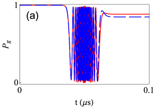
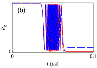
Figure 5: (Color online) $P_{g}$ driven by $H_{RWA}(t)$ (blue dashed line) and by the exact Hamiltonian $H(t)$ (red solid line) for (a) the reference parameters $a=(2\pi)^{2}\times 254.648$ MHz² and $\Omega_{0}=2\pi\times 2$ GHz, and for (b) the optimized parameters $a=(2\pi)^{2}\times 272.824$ MHz² and $\Omega_{0}=2\pi\times 2.202$ GHz, for a population inversion process. In both cases $t_{f}=0.1$ $\mu$s, $\omega_{0}=2\pi\times 5$ GHz, and $A=(2\pi)^{2}\times 506.606$ MHz².

For many field oscillations in the pulse the singularities to avoid in equations (45) and (47) become too numerous to apply the previous approach. A simple inversion method is to assume sensible specific forms with free parameters for the functions $\Delta$ and $\Omega_{R}$. An example is a population inversion process carried out by a linear detuning and a Gaussian Rabi frequency,

$$\Delta(t) = a(t-t_{f}/2),$$ (49)

$$\Omega_{R}(t) = \Omega_{0}\exp[-A(t-t_{f}/2)^{2}],$$

with two free parameters, $a$ and $\Omega_{0}$. For a constant transition (angular) frequency, $\omega_{0}$, taking into account Eqs. (9) and (49), setting $\varphi(0)=\pi/2$ and integrating, the phase of the pulse is given by

$$\varphi(t)=-at^{2}/2+(\omega_{0}+at_{f}/2)t+\pi/2.$$

Setting $\beta(0)=0$, we may solve for $\theta(t)$ and $\beta(t)$ in the system (35), and minimize $[\theta(t_{f})-\pi]^{2}$ numerically to determine $a$ and $\Omega_{0}$. This is a simple alternative to a more sophisticated optimal-control-theory approach scheuer or bang-bang methods avinadav .

In a numerical example we first set the reference parameters, $t_{f}=0.1$ $\mu$s, $\omega_{0}=2\pi\times 5$ GHz, $A=(2\pi)^{2}\times 506.606$ MHz², $a=(2\pi)^{2}\times 254.648$ MHz², and $\Omega_{0}=2\pi\times 2$ GHz, for which the Hamiltonian within and without the RWA give similar dynamics with unsuccessful population inversions, see Fig. 5 (a). For these values of $t_{f}$, $\omega_{0}$, and $A$, and from these seed parameters $a$ and $\Omega_{0}$ a minimization algorithm provides optimized parameters for the population inversion process with the exact Hamiltonian $H(t)$, $a=(2\pi)^{2}\times 272.824$ MHz² and $\Omega_{0}=2\pi\times 2.202$ GHz. The same optimized parameters do not invert the population when the RWA is applied, see Fig. 5 (b).

IV Discussion and conclusions

For a two-level system in a classical field the diagonal and non-diagonal elements in the exact interaction-picture Hamiltonian $H(t)$ must depend consistently on the phase of the field, $\varphi(t)$, and its derivative, $\dot{\varphi}(t)$. This makes the inverse engineering methods more complicated than with the Hamiltonian within the rotating-wave approximation, $H_{RWA}(t)$. Simple attempts using invariants or counterdiabatic methods to implement faster-than-adiabatic processes may not satisfy the consistency condition in $H(t)$ or lead to singularities. Different ways have been shown to circumvent the difficulties. While we have presented simple proof-of-principle examples, the methods may be adapted to minimize effects of noise and decoherence due to the flexibility of the inversion NJP .

An open problem is to extend the approaches to systems where more levels have to be considered. In many systems the failure of the RWA is associated with the need to include further levels in the theoretical treatment. In trapped ions, for example, when the vibrational RWA is not applied, and vibrational counter-rotating terms are taken into account, the energy levels are distorted and the sideband resonances are shifted lizuain . This may be understood as a vibrational Bloch-Siegert effect or, equivalently, as the result of Stark shifts of the levels due to off-resonant transitions lizuain . Nevertheless, it is possible to describe the subspace of the two states in an isolated anticrossing by an approximate $2\times 2$ Hamiltonian that takes into account the effect of further levels perturbatively by means of a level shift operator Cohen ; lizuain . The current approaches could then be applied but the details are left for a separate study.

- (1) E. Torrontegui, S. Ibáñez, S. Martínez-Garaot, M. Modugno, A. del campo, D. Guéry-Odelin, A. Ruschhaupt, X. Chen, and J. G. Muga, Adv. At. Mol. Opt. Phys. 62, 117 (2013).
- (2) X. Sun, H.-C. Liu, and A Yariv, Opt. Lett. 34, 280 (2009).
- (3) T.-Y. Lin, F.-C. Hsiao, Y.-W. Jhang, C. Hu, and S.-Y. Tseng, Opt. Express 20, 24085 (2012).
- (4) S.-Y. Tseng and X. Chen, Opt. Lett. 37, 5118 (2012).
- (5) M. Deschamps, G. Kervern, D. Massiot, G. Pintacuda, L. Emsley, and P. J. Grandinetti, J. Chem. Phys. 129, 204110 (2008).
- (6) E. Collin, G. Ithier, A. Aassime, P. Joyez, D. Vion, and D. Esteve, Phys. Rev. Lett. 93, 157005 (2004).
- (7) B. T. Torosov, S. Guérin, and N. V. Vitanov. Phys. Rev. Lett. 106, 233001 (2011).
- (8) M. Sillanpää, T. Lehtinen, A. Paila, Y. Makhlin, and P. Hakonen, Phys. Rev. Lett. 96, 187002 (2006).
- (9) P. J. Leek, J. M. Fink, A. Blais, R. Bianchetti, M. Göppl, J. M. Gambetta, D. I. Schuster, L. Frunzio, R. J. Schoelkopf, A. Wallraff, Science 318, 1889 (2007).
- (10) X. Chen, E. Torrontegui, and J. G. Muga, Phys. Rev. A 83, 062116 (2011).
- (11) L. Allen and J. H. Eberly, Optical Resonance and Two-level Atoms (Dover, New York, 1987).
- (12) G. D. Fuchs, V. V. Dobrovitski, D. M. Toyli, F. J. Heremans, and D. D. Awschalom, Science 326, 1520 (2009).
- (13) P. London, P. Balasubramanian, B. Naydenov, L. P. McGuinness, and F. Jelezko, Phys. Rev. A 90, 012302 (2014).
- (14) L. Childress and J. McIntyre, Phys. Rev. A 82, 033839 (2010).
- (15) X. Chen, I. Lizuain, A. Ruschhaupt, D. Guéry-Odelin, and J. G. Muga, Phys. Rev. Lett. 105, 123003 (2010).
- (16) J. Zhang, J. H. Shim, I. Niemeyer, T. Taniguchi, T. Teraji, H. Abe, S. Onoda, T. Yamamoto, T. Ohshima, J. Isoya, and D. Suter, Phys. Rev. Lett. 110, 240501 (2013).
- (17) M. Demirplak and S. A. Rice, J. Phys. Chem. A 107, 9937 (2003).
- (18) M. Demirplak and S. A. Rice, J. Phys. Chem. B 109, 6838 (2005).
- (19) M. Demirplak and S. A. Rice, J. Chem. Phys. 129, 154111 (2008).
- (20) M. V. Berry, J. Phys. A: Math. Theor. 42, 365303 (2009).
- (21) S. Ibáñez, X. Chen, E. Torrontegui, J. G. Muga, and A. Ruschhaupt, Phys. Rev. Lett. 109, 100403 (2012).
- (22) H. R. Lewis and W. B. Riesenfeld, J. Math. Phys. 10, 1458 (1969).
- (23) S. Ibáñez, A. Peralta Conde, D. Guéry-Odelin, and J. G. Muga, Phys. Rev. A 84, 013428 (2011).
- (24) J. Chen and L. F. Wei, Phys. Rev. A 91, 023405 (2015).
- (25) Y.-Z. Lai, J.-Q. Liang, H. J. W. Müller-Kirsten, and J.-G. Zhou, Phys. Rev. A 53, 3691 (1996).
- (26) Y.-Z. Lai, J.-Q. Liang, H. J. W. Müller-Kirsten, and J.-G. Zhou, J. Phys. A: Math. Gen. 29, 1773 (1996).
- (27) T. Ackemann, A. Heuer, Yu A. Logvin, and W. Lange, Phys. Rev. A 56, 2321 (1997).
- (28) J. Scheuer, Xi Kong, R. S. Said, J. Chen, A. Kurz, L. Marseglia, J. Du, P. R. Hemmer, S. Montangero, T. Calarco, B. Naydenov, and F. Jelezko, New J. Phys. 16, 093022 (2014).
- (29) C. Avinadav, R. Fischer, P. London, and D. Gershoni, Phys. Rev. B 89, 245311 (2014).
- (30) A. Ruschhaupt, X. Chen, D. Alonso, and J. G. Muga, New J. Phys. 14, 093040 (2012).
- (31) I. Lizuain, J. G. Muga, and J. Eschner, Phys. Rev. A 77, 053817 (2008).
- (32) C. Cohen-Tannoudji, J. Dupont-Roc, and G. Grynberg, Atom-Photon Interactions, Wiley, New York, 1998.