Imaging with power controlled source pairs

Abstract.

Scatterers in a homogeneous medium are imaged by probing the medium with two point sources of waves modulated by correlated signals and by measuring only intensities at one single receiver. For appropriately chosen source pairs, we show that full waveform array measurements can be recovered from such intensity measurements by solving a linear least squares problem. The least squares solution can be used to image with Kirchhoff migration, even if the solution is determined only up to a known one-dimensional nullspace. The same imaging strategy can be used when the medium is probed with point sources driven by correlated Gaussian processes and autocorrelations are measured at a single location. Since autocorrelations are robust to noise, this can be used for imaging when the probing wave is drowned in background noise.

Keywords. Intensity-only imaging, travel-time migration, noise sources, autocorrelation.

AMS Subject Classifications. 78A45, 78A46, 35R30

1. Introduction

Scatterers in a homogeneous medium can be imaged by probing the medium with a wave emanating from a point source, and recording the reflected waves at one or more receivers. An image of the scatterers can be generated by repeating this experiment while varying the position of the source and/or receiver and using classic methods such as the Kirchhoff (travel time) migration (see e.g. [1]) or MUSIC (see e.g. [6]). We are concerned here with the case where only intensity measurements can be made at the receiver; destroying phase information that migration and MUSIC need to image. Intensity measurements occur e.g. when the response time of the receiver is larger than the typical wave period or when it is more cost effective to measure intensities than the full waveform. This is typical in e.g. optical coherence tomography [24, 23] and radar imaging [7]. Another situation is when the wave sources are stochastic and the measurements consist of correlations of the signal recorded at different points [27, 10]. In the special case of autocorrelations (i.e. correlating the signal with itself), the Wiener-Khinchin theorem guarantees we are measuring power spectra (see e.g. [18]), another form of intensity measurements.

The setup we analyze consists of an array of sources and one single receiver that can only record power spectra, i.e. the intensity of the signal at certain frequency samples. A crucial assumption for our method is that we can use source pairs, meaning we can send correlated signals from two different locations. Thus we allow for known delays or attenuations between the signals in a source pair. In acoustics, one way of achieving this would be to drive two transducers in an array with the same signal. With light, one could use an incoherent plane wave with wavefronts parallel to a configurable mask. The mask lets light through one or two small holes, whose locations can be controlled.

Our method can be used for imaging from both measurements of intensities (§1.1) and autocorrelations (§1.2).

1.1. Intensity only measurements

One way to deal with intensity measurements is phase retrieval, i.e. first recovering the phases from intensity measurements, and using this reconstructed field to image. In diffraction tomography, intensity measurements at two different planes can be used to recover phases [16, 29, 15]. If additional information is known (e.g. the support of the scatterer), intensities at one single plane can be used [9, 20, 19]. Total or partial knowledge of the incident field can also be exploited to image from intensities at one single plane [8].

Chai et al. [4] take a compressed sensing approach to image a few point scatterers exactly. With knowledge of the incident field, the location of the scatterers can be resolved in both range and cross-range with monochromatic measurements. The same ideas can even be used to deal with multiple scattering [5]. Novikov et al. [21] use the polarization identity $4\text{Re}(\bm{u}^{*}\bm{v})=\|\bm{u}+\bm{v}\|^{2}-\|\bm{u}-\bm{v}\|^{2}$, $\bm{u},\bm{v}\in\mathbb{C}^{N}$, and linear combinations of single source experiments to recover dot products of two single source experiments from intensity data. MUSIC can then be used to image with this quadratic functional of the full waveform data.

Here we do phase retrieval assuming knowledge of the intensity of the incident field. Our illumination strategy using source pairs does not require direct manipulation of phases or addition/subtraction of wave fields. We reduce the recovery of the total field to a linear system with a one-dimensional nullspace which we can write explicitly in terms of the incident field. There is one (very sparse) linear system per frequency sample to solve, and the linear system has size comparable to twice the number of source positions. Intuitively we are recovering a field in $\mathbb{C}^{N}$ from $2N$ (or more) real measurements. We show that vectors in the one-dimensional nullspace do not affect Kirchhoff migration. Hence we can use, without modification, Kirchhoff migration and its standard range and cross-range resolution estimates (see e.g. [1]).

1.2. Correlation based methods

In seismic imaging, correlations of traces (or recordings) at many receivers have been used to image the earth’s subsurface, especially when the wave sources and their locations are not well known [25, 27, 26]. The idea is that correlations of the signals at two different locations contain information about the Green’s function between the two locations, and this information can be exploited to image the medium and any scatterers. This principle can even be exploited to do opportunistic imaging with ambient noise [10, 11, 14]. Cross-correlations can also be used to image scatterers in a random medium [3, 12, 13]. In radar imaging, the measurements are in fact correlations [7], and so even stochastic processes can be used instead of deterministic signals [28, 30].

The method we present here can also be used to image scatterers using autocorrelations. We show it is possible to form an image by exploiting angular diversity in source pairs instead of cross-correlations among different receivers. Just as in the intensity measurements case, we are able to recover (up to a one dimensional nullspace) full waveform array measurements. One advantage of using autocorrelations instead of cross-correlations is that the data acquisition at the (single) receiver is simpler. The drawback is that our illumination strategy requires to illuminate with pairs of sources, but also with each of the sources in a pair on its own. To get the same full waveform data as an array with $N$ sources, we need at least $3N$ different experiments. Another advantage of using autocorrelations is that the measurements are extremely robust to noise. As an example, our numerical experiments show that it is possible to image scatterers with an array that is sending noise from all possible source positions; the only assumption about the noise being that all the sources are independent stochastic processes except for two correlated sources whose positions we can control. Because of this robustness, it may be possible to use our imaging method in situations where the medium is to be probed in a non-intrusive way, i.e. active imaging with waves that are of the same magnitude as the ambient noise.

1.3. Contents

The particular physical setup we consider is described in §2. The illumination strategy with source pairs is explained in §3, which leads to a phase retrieval problem that can be formulated as a linear system (§4). The least squares solution to the linear system is then used as data for imaging with Kirchhoff migration, and we show that this gives essentially the same images as full waveform data (§5). The extension to stochastic source pairs is given in §6. Then we show that our method is robust to additive noise when using autocorrelations (§7). Numerical experiments illustrating our method are given in §8 and we conclude with a discussion in §9.

2. Array imaging for full waveform measurements

Here we introduce the experimental setup we consider (§2.1) and briefly recall the classic Kirchhoff migration imaging method (§2.2).

2.1. Experimental setup

The physical setup is illustrated in figure 1. We probe a homogeneous medium with waves originating from $N$ point sources with locations $\vec{\bm{x}}_{s}\in\mathcal{A}$, $s=1,2,\ldots,N$. For simplicity we consider a linear array in 2D or a square array in 3D, i.e. $\mathcal{A}=[-a/2,a/2]^{d-1}\times\{0\}$, where $d=2$ or $3$ is the dimension. Our imaging strategy imposes only mild restrictions on the source positions, so other array shapes may be considered. Waves are recorded at a single known receiver location $\vec{\bm{x}}_{r}$.

The total field generated by the array (or incident field) can be written as

(1) $$\widehat{u}_{\text{inc}}(\vec{\bm{x}},\omega)=\bm{g}_{0}(\vec{\bm{x}},\omega)^{\mathsf{T}}\bm{f}(\omega),$$

where

(2) $$\bm{g}_{0}(\vec{\bm{x}},\omega)=\begin{bmatrix}\widehat{G}_{0}(\vec{\bm{x}},\vec{\bm{x}}_{1},\omega),\widehat{G}_{0}(\vec{\bm{x}},\vec{\bm{x}}_{2},\omega),\ldots,\widehat{G}_{0}(\vec{\bm{x}},\vec{\bm{x}}_{N},\omega)\end{bmatrix}^{\mathsf{T}}\in\mathbb{C}^{N},$$

and the source driving signals are $\bm{f}(\omega)=[\widehat{f}_{1}(\omega),\widehat{f}_{2}(\omega),\ldots,\widehat{f}_{N}(\omega)]^{\mathsf{T}}$. Since we assume waves propagate through a homogeneous medium, we used the outgoing free space Green function,

(3) $$\widehat{G}_{0}(\vec{\bm{x}},\vec{\bm{y}},\omega)=\begin{cases}\frac{\imath}{4}H_{0}^{(1)}(k|\vec{\bm{x}}-\vec{\bm{y}}|),&\text{for $d=2$},\\ \displaystyle\frac{\exp[\imath k|\vec{\bm{x}}-\vec{\bm{y}}|]}{4\pi|\vec{\bm{x}}-\vec{\bm{y}}|},&\text{for $d=3$.}\end{cases}$$

Here $H_{0}^{(1)}$ is the zeroth order Hankel function of the first kind, $k=\omega/c_{0}$ is the wavenumber, $\omega$ is the angular frequency and $c_{0}$ is a known constant background wave speed. For functions of time, the Fourier transform convention we use is

(4) $$\widehat{f}(\omega)=\int f(t)e^{\imath\omega t}dt,~{}\text{and}~{}f(t)=\frac{1}{2\pi}\int\widehat{f}(\omega)e^{-\imath\omega t}d\omega,~{}\text{where $f\in L^{2}(\mathbb{R})$.}$$

The scatterers we want to image are represented by a compactly supported reflectivity function $\rho(\vec{\bm{x}})$. Under the weak scattering assumption (i.e. $\rho\ll 1$), we can use the Born approximation to the total field at the receiver

(5) $$\widehat{u}(\vec{\bm{x}}_{r},\omega)=(\bm{g}_{0}+\bm{p})^{\mathsf{T}}\bm{f},$$

where the array response vector is

(6) $$\bm{p}(\vec{\bm{x}},\omega)=k^{2}\int d\vec{\bm{y}}\rho(\vec{\bm{y}})\widehat{G}_{0}(\vec{\bm{x}},\vec{\bm{y}},\omega)\bm{g}_{0}(\vec{\bm{y}},\omega).$$

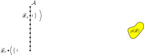
Figure 1. Physical setup for array imaging with an array $\mathcal{A}$ of sources $\vec{\bm{x}}_{s}$ and a single receiver $\vec{\bm{x}}_{r}$. The scatterer is represented by a compactly supported reflectivity function $\rho(\vec{\bm{x}})$.

2.2. Kirchhoff migration

By e.g. using illuminations $\bm{f}(\omega)=\bm{e}_{i}$, $i=1,\ldots,N$ corresponding to the canonical basis vectors, it is possible to obtain the array response vector $\bm{p}(\vec{\bm{x}}_{r},\omega)$ from the measurements (5). The scatterers can then be imaged using the Kirchhoff migration functional (see e.g. [1]) which for a single frequency $\omega$ is

(7) $$\Gamma_{\text{KM}}[\bm{p},\omega](\vec{\bm{y}})=\overline{\widehat{G}}_{0}(\vec{\bm{y}},\vec{\bm{x}}_{r},\omega)\bm{g}_{0}(\vec{\bm{y}},\omega)^{*}\bm{p}(\vec{\bm{x}}_{r},\omega),$$

where $\vec{\bm{y}}$ represents a point in the image. This image has a Rayleigh or cross-range (i.e. in the direction parallel to the array) resolution of $\lambda L/a$, where $L$ is the distance from the array to the scatterer (see e.g. [1]). To get range (i.e. in the direction perpendicular to the array) resolution we need to integrate $\Gamma_{\text{KM}}[\bm{p},\omega](\vec{\bm{y}})$ for frequencies $\omega$ in some frequency band $\mathcal{B}=[-\omega_{max},-\omega_{min}]\cup[\omega_{min},\omega_{max}]$, the same frequency band of the signals $\bm{f}(\omega)$. The range resolution is then $c_{0}/(\omega_{max}-\omega_{min})$ (see e.g. [1]). We discuss this imaging functional further in section 5.

3. Intensity only measurements

We start in §3.1 by describing a source pair illumination strategy for intensity measurements of the total field $|\widehat{u}(\vec{\bm{x}}_{r},\omega)|^{2}$. With this strategy, the problem of recovering the array response vector $\bm{p}$ can be formulated as a linear system (§3.2).

3.1. Illumination strategy

The data we use comes from probing the medium with $N_{p}$ source pairs that are sending signals with known power and phase difference. Since the number of distinct source pairs out of an array with $N$ sources is $N(N-1)/2$ we must have $N_{p}\leq N(N-1)/2$. We assume the power and phase differences remain the same for all $N_{p}$ illuminations. The case where these quantities depend on the source pair is left for future studies. To be more precise, the illumination corresponding to the $m-$th source pair $(i(m),j(m))\in\{1,\ldots,N\}^{2}$ is

(8) $$\bm{f}_{m}(\omega)=\mathsf{F}_{m}\begin{bmatrix}\alpha(\omega)\\ \beta(\omega)\end{bmatrix},~{}\text{where}~{}\mathsf{F}_{m}=[\bm{e}_{i(m)},\bm{e}_{j(m)}]\in\mathbb{R}^{N\times 2}.$$

We emphasize that only $|\alpha|^{2}$, $|\beta|^{2}$ and the phase difference $\phi(\omega)\equiv\arg(\overline{\alpha}\beta)$ is assumed to be known for the signals $\alpha$ and $\beta$. A particular case is when the same signal is sent from the source pair, i.e. $\beta=\alpha$ and $\phi(\omega)=0$.

The intensity of the field $u_{m}$ arising from the source pair illumination $\bm{f}_{m}$ is

(9) $$|\widehat{u}_{m}(\vec{\bm{x}}_{r},\omega)|^{2}=\overline{\bm{g}^{\mathsf{T}}\bm{f}_{m}}\bm{f}_{m}^{\mathsf{T}}\bm{g}=\bm{g}^{*}\mathsf{F}_{m}\begin{bmatrix}|\alpha|^{2}&\overline{\alpha}\beta\\ \overline{\beta}\alpha&|\beta|^{2}\end{bmatrix}\mathsf{F}_{m}^{\mathsf{T}}\bm{g},$$

where we used $\bm{g}=\bm{g}_{0}+\bm{p}$. Note that since $\overline{\alpha}\beta=|\alpha||\beta|e^{\imath\phi}$, the inner $2\times 2$ Hermitian matrix is uniquely determined by the magnitudes of $\alpha$ and $\beta$ and their phase difference $\phi$. By using the single source reference illumination $\bm{e}_{i}$ we additionally measure

(10) $$|\widehat{u}_{i}^{0}(\vec{\bm{x}}_{r},\omega)|^{2}=\bm{g}^{*}\bm{e}_{i}\bm{e}_{i}^{\mathsf{T}}\bm{g},\qquad\text{ for $i=1,\ldots,N.$}$$

The data we exploit to recover $\bm{p}$ is obtained by subtracting the appropriate reference illuminations (10) from (9), that is

$$d_{m}(\vec{\bm{x}}_{r},\omega) =|\widehat{u}_{m}|^{2}-|\alpha|^{2}|\widehat{u}_{i(m)}^{0}|^{2}-|\beta|^{2}|\widehat{u}_{j(m)}^{0}|^{2}$$

$$=\bm{g}^{*}\mathsf{F}_{m}\begin{bmatrix}0&\overline{\alpha}\beta\\ \overline{\beta}\alpha&0\end{bmatrix}\mathsf{F}_{m}^{\mathsf{T}}\bm{g}.$$

3.2. Phase retrieval problem as a linear system

By recalling that $\bm{g}=\bm{g}_{0}+\bm{p}$, the measurements $d_{m}$ are

$$d_{m}(\vec{\bm{x}}_{r},\omega)=(\bm{g}_{0}+\bm{p})^{*}\mathsf{F}_{m}\begin{bmatrix}0&\overline{\alpha}\beta\\ \overline{\beta}\alpha&0\end{bmatrix}\mathsf{F}_{m}^{\mathsf{T}}(\bm{g}_{0}+\bm{p}).$$

To make the following expressions concise, we denote by $\mathsf{D}$ the Hermitian matrix

(11) $$\mathsf{D}=\begin{bmatrix}0&\overline{\alpha}\beta\\ \overline{\beta}\alpha&0\end{bmatrix}.$$

By the weak scattering assumption, we may neglect the quadratic terms in $\bm{p}$ and collect all measurements for $m=1,\ldots,N_{p}$ as a single vector $\bm{d}\in\mathbb{R}^{N_{p}}$:

(12) $$\begin{bmatrix}d_{1}(\vec{\bm{x}}_{r},\omega)\\ d_{2}(\vec{\bm{x}}_{r},\omega)\\ \vdots\\ d_{N_{p}}(\vec{\bm{x}}_{r},\omega)\\ \end{bmatrix}\approx\bm{d}(\vec{\bm{x}}_{r},\omega) =\text{Re}\begin{pmatrix}\begin{bmatrix}\bm{g}_{0}^{*}\mathsf{F}_{1}\mathsf{D}\mathsf{F}_{1}^{\mathsf{T}}\\ \bm{g}_{0}^{*}\mathsf{F}_{2}\mathsf{D}\mathsf{F}_{2}^{\mathsf{T}}\\ \vdots\\ \bm{g}_{0}^{*}\mathsf{F}_{N_{p}}\mathsf{D}\mathsf{F}_{N_{p}}^{\mathsf{T}}\end{bmatrix}(\bm{g}_{0}+2\bm{p})\end{pmatrix}$$

$$=\mathsf{M}(\vec{\bm{x}}_{r},\omega)\begin{bmatrix}\text{Re}(\bm{g}_{0}+2\bm{p})\\ \text{Im}(\bm{g}_{0}+2\bm{p})\end{bmatrix},$$

where the $N_{p}\times 2N$ real matrix $\mathsf{M}$ is given by

(13) $$\mathsf{M}(\vec{\bm{x}}_{r},\omega)=\begin{bmatrix}\text{Re}(\bm{g}_{0}^{*}\mathsf{F}_{1}\mathsf{D}\mathsf{F}_{1}^{\mathsf{T}})&-\text{Im}(\bm{g}_{0}^{*}\mathsf{F}_{1}\mathsf{D}\mathsf{F}_{1}^{\mathsf{T}})\\ \text{Re}(\bm{g}_{0}^{*}\mathsf{F}_{2}\mathsf{D}\mathsf{F}_{2}^{\mathsf{T}})&-\text{Im}(\bm{g}_{0}^{*}\mathsf{F}_{2}\mathsf{D}\mathsf{F}_{2}^{\mathsf{T}})\\ \vdots&\vdots\\ \text{Re}(\bm{g}_{0}^{*}\mathsf{F}_{N_{p}}\mathsf{D}\mathsf{F}_{N_{p}}^{\mathsf{T}})&-\text{Im}(\bm{g}_{0}^{*}\mathsf{F}_{N_{p}}\mathsf{D}\mathsf{F}_{N_{p}}^{\mathsf{T}})\\ \end{bmatrix}.$$

Note that by construction, the matrix $\mathsf{M}$ has at most 4 non-zero elements per row, and is thus a very sparse matrix for $N$ large.

4. Analysis of the phase retrieval linear system

We now address the question of whether there is enough information in the measurements $\bm{d}\in\mathbb{R}^{N_{p}}$ to recover the array response vector $\bm{p}\in\mathbb{C}^{N}$. The main result of this section is Theorem 4.3, where we show that with appropriately chosen pairs of sources, $\mathsf{M}^{\dagger}\bm{d}$ (i.e. the Moore Penrose pseudoinverse of $\mathsf{M}$ times $\bm{d}$) gives $\bm{p}$ up to a complex scalar multiple of the vector $\bm{g}_{0}$, which is known a priori.

Let us first consider the case where we take measurements using all possible source pairs, i.e. that $N_{p}=N(N-1)/2$. Clearly, we need $N\geq 5$ to guarantee that $N_{p}\geq 2N$, i.e. that the matrix $\mathsf{M}$ has more rows than columns and the system $\bm{d}=\mathsf{M}[\text{Re}(\bm{g}_{0}+2\bm{p})^{\mathsf{T}},\text{Im}(\bm{g}_{0}+2\bm{p})^{\mathsf{T}}]^{\mathsf{T}}$ is overdetermined.

Instead of using all possible source pairs, we use the following strategy which for $N\geq 5$, guarantees $N_{p}=2N$.

Strategy to choose source pairs:

1. All 10 distinct source pairs between the source positions $\{1,\ldots,5\}$.

2. For source position $s>5$, choose any two different source pairs of the form $(s,i)$ and $(s,j)$ where $i,j\in\{1,\ldots,5\}$.

This strategy is illustrated in figure 2. More source pairs can be added without affecting the recoverability of $\bm{p}$ (Theorem 4.3). We now make the following assumption on the first 5 source positions.

Figure 2. An example illustrating the strategy to choose the source pairs for $N=8$ source positions. Each source position is represented by a node in the graph, and source pairs are represented by edges. The first 5 source positions are in the circle.

Assumption 4.1.

We assume the receiver is located at a position $\vec{\bm{x}}_{r}$ such that for $i,j=1,\ldots,5$, the vector $\bm{g}_{0}\equiv\bm{g}_{0}(\vec{\bm{x}}_{r},\omega)$ satisfies

(14) $$\text{Re}\big{(}\bm{g}_{0}\big{)}_{i}\neq 0,~{}\text{Im}\big{(}\bm{g}_{0}\big{)}_{i}\neq 0,~{}\text{and}~{}\text{Re}\big{(}\bm{g}_{0}\big{)}_{i}\text{Im}\big{(}\bm{g}_{0}\big{)}_{j}\neq\text{Re}\big{(}\bm{g}_{0}\big{)}_{j}\text{Im}\big{(}\bm{g}_{0}\big{)}_{i}.$$

Additionally for one pair $i,j\in[1,\ldots,5]$ we assume

(15) $$\cos(\phi) \left(\text{Re}\big{(}\bm{g}_{0}\big{)}_{i}\text{Im}\big{(}\bm{g}_{0}\big{)}_{j}-\text{Re}\big{(}\bm{g}_{0}\big{)}_{j}\text{Im}\big{(}\bm{g}_{0}\big{)}_{i}\right)\neq$$

$$\qquad\qquad-\sin(\phi)\left(\text{Re}\big{(}\bm{g}_{0})_{i}\text{Re}\big{(}\bm{g}_{0}\big{)}_{j}+\text{Im}\big{(}\bm{g}_{0}\big{)}_{i}\text{Im}\big{(}\bm{g}_{0}\big{)}_{j}\right).$$

This assumption is by no means necessary for the end result (Theorem 4.3) to hold, but it is sufficient. If $d=3$, condition (14) is equivalent to the geometric condition

(16) $$|\vec{\bm{x}}_{i}-\vec{\bm{x}}_{r}|\notin\frac{\lambda}{4}\mathbb{Z}~{}\text{and}~{}|\vec{\bm{x}}_{i}-\vec{\bm{x}}_{r}|-|\vec{\bm{x}}_{j}-\vec{\bm{x}}_{r}|\notin\frac{\lambda}{2}\mathbb{Z}~{}\text{for all $i,j=1,\ldots,5$},$$

while condition (15) implies for one pair $i,j\in[1,\ldots,5]$ that

(17) $$|\vec{\bm{x}}_{r}-\vec{\bm{x}}_{i}|-|\vec{\bm{x}}_{r}-\vec{\bm{x}}_{j}|\notin\frac{\lambda}{2}\mathbb{Z}-\frac{\lambda}{2\pi}\phi.$$

Here the set $(\lambda/2)\mathbb{Z}$ is the set of all integer multiples of $\lambda/2$, where $\lambda=2\pi c_{0}/\omega$ is the wavelength. In $d=2$, conditions similar to (16) and (17) are sufficient when the sources and receivers are far apart because of the Hankel function asymptotic

$$H_{0}^{(1)}(t)=\sqrt{\frac{2}{\pi t}}\exp[\imath(t-(\pi/4))](1+\mathcal{O}(1/t)),~{}\text{as $t\to\infty$}.$$

Lemma 4.2.

Provided $\alpha\neq 0$, $\beta\neq 0$, $\text{Re}(\overline{\alpha}\beta)\neq 0$, the source pairs are chosen with the above strategy and assumption 4.1 holds, the matrix $\mathsf{M}\equiv\mathsf{M}(\vec{\bm{x}}_{r},\omega)$ satisfies

(18) $$\operatorname{null}\mathsf{M}=\operatorname{span}\left\{\begin{bmatrix}-\text{Im}\big{(}\bm{g}_{0}(\vec{\bm{x}}_{r},\omega)\big{)}\\ \text{Re}\big{(}\bm{g}_{0}(\vec{\bm{x}}_{r},\omega)\big{)}\end{bmatrix}\right\}.$$

Proof.

For clarity of exposition, we adopt the notation

$$a_{i}=\text{Re}\big{(}\bm{g}_{0}\big{)}_{i},~{}b_{i}=\text{Im}\big{(}\bm{g}_{0}\big{)}_{i},$$

for $i=1,\ldots,N$ and with $\bm{g}_{0}\equiv\bm{g}_{0}(\vec{\bm{x}}_{r},\omega)$. The proposed vector spanning the nullspace is $[\bm{v}^{\mathsf{T}},\bm{w}^{\mathsf{T}}]^{\mathsf{T}}=[-\text{Im}(\bm{g}_{0})^{\mathsf{T}},\text{Re}(\bm{g}_{0})^{\mathsf{T}}]^{\mathsf{T}}$ and has components $v_{i}=-b_{i}$ and $w_{i}=a_{i}$ for $i=1,\ldots,N$.

The proof is by induction on the number of sources $N$. For the purpose of the induction argument, we denote by $\mathsf{M}^{(N)}$ the measurement matrix $\mathsf{M}(\vec{\bm{x}_{r}},\omega)$ corresponding to $N$ sources, which if we use the strategy explained above, must be a $2N\times 2N$ real matrix. For the base case $N=5$ of the induction, $\mathsf{M}^{(5)}$ can be written as

$$\mathsf{M}^{(5)}=\begin{bmatrix}A_{2}^{-}&A_{1}^{+}&0&0&0&B_{2}^{+}&B_{1}^{-}&0&0&0\\ A_{3}^{-}&0&A_{1}^{+}&0&0&B_{3}^{+}&0&B_{1}^{-}&0&0\\ A_{4}^{-}&0&0&A_{1}^{+}&0&B_{4}^{+}&0&0&B_{1}^{-}&0\\ A_{5}^{-}&0&0&0&A_{1}^{+}&B_{5}^{+}&0&0&0&B_{1}^{-}\\ 0&A_{3}^{-}&A_{2}^{+}&0&0&0&B_{3}^{+}&B_{2}^{-}&0&0\\ 0&A_{4}^{-}&0&A_{2}^{+}&0&0&B_{4}^{+}&0&B_{2}^{-}&0\\ 0&A_{5}^{-}&0&0&A_{2}^{+}&0&B_{5}^{+}&0&0&B_{2}^{-}\\ 0&0&A_{4}^{-}&A_{3}^{+}&0&0&0&B_{4}^{+}&B_{3}^{-}&0\\ 0&0&A_{5}^{-}&0&A_{3}^{+}&0&0&B_{5}^{+}&0&B_{3}^{-}\\ 0&0&0&A_{5}^{-}&A_{4}^{+}&0&0&0&B_{5}^{+}&B_{4}^{-}\\ \end{bmatrix},$$

where we have used

(19) $$A_{i}^{\pm} =|\alpha||\beta|(\cos(\phi)a_{i}\pm\sin(\phi)b_{i}),\qquad B_{i}^{\pm} =|\alpha||\beta|(\cos(\phi)b_{i}\pm\sin(\phi)a_{i}).$$

Using the expressions (19), the leading principal $9\times 9$ minor of $\mathsf{M}^{(5)}$ is

$$|\mathsf{M}_{1:9,1:9}^{(5)}| =-4|\alpha|^{9}|\beta|^{9}\cos^{2}(\phi)\left(\cos(\phi)(b_{3}a_{1}-b_{1}a_{3})+\sin(\phi)(b_{3}b_{1}+a_{3}a_{1})\right)\times$$

$$\qquad a_{5}(b_{3}a_{2}-b_{2}a_{3})(b_{2}a_{1}-a_{2}b_{1})(b_{5}a_{4}-a_{5}b_{4}).$$

Therefore if assumption 4.1 holds and $\cos\phi\neq 0$ (which we get from $\text{Re}(\overline{\alpha}\beta)\neq 0$), we must have $\operatorname{rank}\mathsf{M}^{(5)}\geq 9$. By direct calculations, we have that

$$\operatorname{null}\mathsf{M}^{(5)}=\operatorname{span}\left\{[-b_{1},\ldots,-b_{5},a_{1},\ldots,a_{5}]^{\mathsf{T}}\right\}.$$

Thus the base case $N=5$ holds and $\operatorname{rank}\mathsf{M}^{(5)}=9$.

For the induction hypothesis we assume that $N\geq 5$ and that

$$\operatorname{null}\mathsf{M}^{(N)}=\operatorname{span}\left\{[-\bm{b}^{\mathsf{T}},\bm{a}^{\mathsf{T}}]^{\mathsf{T}}\right\},$$

where $\bm{a}=[a_{1},\ldots,a_{N}]^{\mathsf{T}}$ and $\bm{b}=[b_{1},\ldots,b_{N}]^{\mathsf{T}}$. If the first $2N$ source pairs to construct $\mathsf{M}^{(N+1)}$ are chosen in exactly the same way as the source pairs to construct $\mathsf{M}^{(N)}$, and the last two source pairs are, e.g. $(N+1,1)$ and $(N+1,2)$ we must have for any $\bm{v},\bm{w}\in\mathbb{R}^{N}$ and $v_{N+1},w_{N+1}\in\mathbb{R}$ that

(20) $$\mathsf{M}^{(N+1)}\begin{bmatrix}\bm{v}\\ v_{N+1}\\ \bm{w}\\ w_{N+1}\end{bmatrix}=\begin{bmatrix}\mathsf{M}^{(N)}\begin{bmatrix}\bm{v}\\ \bm{w}\end{bmatrix}\\ A_{N+1}^{-}v_{1}+A_{1}^{+}v_{N+1}+B_{N+1}^{+}w_{1}+B_{1}^{-}w_{N+1}\\ A_{N+1}^{-}v_{2}+A_{2}^{+}v_{N+1}+B_{N+1}^{+}w_{2}+B_{2}^{-}w_{N+1}\end{bmatrix}.$$

Hence if $[\bm{v}^{\mathsf{T}},v_{N+1},\bm{w}^{\mathsf{T}},w_{N+1}]^{\mathsf{T}}\in\operatorname{null}\mathsf{M}^{(N+1)}$, then we must have $[\bm{v}^{\mathsf{T}},\bm{w}^{\mathsf{T}}]^{\mathsf{T}}\in\operatorname{null}\mathsf{M}^{(N)}$, i.e. there is some real $k\neq 0$ such that $\bm{v}=-k\bm{b}$ and $\bm{w}=k\bm{a}$. Equating the last two components of (20) to zero and using that $v_{i}=-kb_{i}$ and $w_{i}=ka_{i}$ for $i=1,2$, one gets the linear system

$$\begin{bmatrix}A_{1}^{+}&B_{1}^{-}\\ A_{2}^{+}&B_{2}^{-}\end{bmatrix}\begin{bmatrix}v_{N+1}\\ w_{N+1}\end{bmatrix}=\begin{bmatrix}kA_{N+1}^{-}b_{1}-kB_{N+1}^{+}a_{1}\\ kA_{N+1}^{-}b_{2}-kB_{N+1}^{+}a_{2}\end{bmatrix}.$$

Since $A_{1}^{+}B_{2}^{-}-A_{2}^{+}B_{1}^{-}=|\alpha|^{2}|\beta|^{2}(a_{1}b_{2}-a_{2}b_{1})\neq 0$, the unique solution to this system is $v_{N+1}=-kb_{N+1}$ and $w_{N+1}=ka_{N+1}$. Thus the desired result holds for any $N\geq 5$. ∎

In figure 3, we show the condition number of $\mathsf{M}(\vec{\bm{x}}_{r},\omega)$ (i.e. $\sigma_{1}/\sigma_{2N-1}$ the ratio of the largest singular value to the smallest non-zero singular value ) over a frequency band. The experimental setup is that given in §8 and corresponds to sending exactly the same signal from both locations in a source pair (i.e. $\alpha=\beta$ and $\phi=0$). Figure 3(a) shows the condition number of $\mathsf{M}$ with $\vec{\bm{x}}_{r}$ chosen so that assumption 4.1 is satisfied, while figure 3(b) shows the condition number of $\mathsf{M}$ with $\vec{\bm{x}}_{r}$ chosen so that assumption 4.1 is violated for some frequencies. In both cases, we see improved conditioning by using more than $2N$ source pair experiments.

(a)	(b)

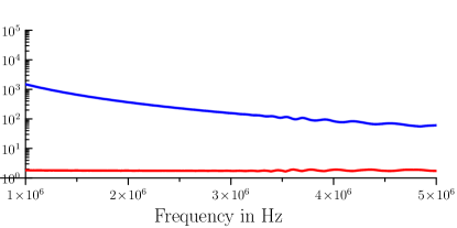
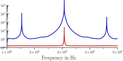
Figure 3. Condition number of $\mathsf{M}(\vec{\bm{x}}_{r},\omega)$ with receiver location $\vec{\bm{x}}_{r}$ chosen so that (a) assumption 4.1 is satisfied, (b) assumption 4.1 is violated for some frequencies. The number of source pair experiments used is $N_{p}=N(N-1)/2$ (in red) and $N_{p}=2N$ (in blue).

We now tie $\mathsf{M}^{\dagger}\bm{d}$ to the array response vector $\bm{p}$.

Theorem 4.3.

Under the assumptions of lemma 4.2 it is possible to recover $\bm{p}\equiv\bm{p}(\vec{\bm{x}}_{r},\omega)$ from the intensity data $\bm{d}$ up to a complex scalar multiple of $\bm{g}_{0}\equiv\bm{g}_{0}(\vec{\bm{x}}_{r},\omega)$, more precisely, $\mathsf{M}^{\dagger}\bm{d}$ determines the vector $\bm{p}+\zeta\bm{g}_{0}$ where

(21) $$\zeta\equiv\zeta(\vec{\bm{x}}_{r},\omega)=\frac{1}{2}-\imath\frac{\text{Im}(\bm{g}_{0}^{*}\bm{p})}{\bm{g}_{0}^{*}\bm{g}_{0}}.$$

Proof.

Recalling the form of our data we have

$$\bm{d}=\mathsf{M}\begin{bmatrix}\text{Re}\big{(}\bm{g}_{0}+2\bm{p}\big{)}\\ \text{Im}\big{(}\bm{g}_{0}+2\bm{p}\big{)}\end{bmatrix}.$$

By lemma 4.2, the matrix $\mathsf{M}$ has a one dimensional nullspace therefore

$$\mathsf{M}^{\dagger}\bm{d}=\begin{bmatrix}\text{Re}(\bm{g}_{0}+2\bm{p})\\ \text{Im}(\bm{g}_{0}+2\bm{p})\end{bmatrix}-\tilde{\zeta}\begin{bmatrix}-\text{Im}(\bm{g}_{0})\\ \text{Re}(\bm{g}_{0})\end{bmatrix},$$

where $\tilde{\zeta}\in\mathbb{R}$ is found by enforcing orthogonality with $[-\text{Im}(\bm{g}_{0})^{\mathsf{T}},\text{Re}(\bm{g}_{0})^{\mathsf{T}}]^{\mathsf{T}}$, i.e.

$$\tilde{\zeta}=\frac{1}{\bm{g}_{0}^{*}\bm{g}_{0}}[-\text{Re}(\bm{g}_{0}+2\bm{p})^{\mathsf{T}}\text{Im}(\bm{g}_{0})+\text{Im}(\bm{g}_{0}+2\bm{p})^{\mathsf{T}}\text{Re}(\bm{g}_{0})]=\frac{2\text{Im}(\bm{g}_{0}^{*}\bm{p})}{\bm{g}_{0}^{*}\bm{g}_{0}}.$$

Thus from $\mathsf{M}^{\dagger}\bm{d}$ we can get the $\mathbb{C}^{N}$ vector

$$\frac{1}{2}[\text{Re}(\bm{g}_{0}+2\bm{p})+\tilde{\zeta}\text{Im}(\bm{g}_{0})]+\frac{\imath}{2}[\text{Im}(\bm{g}_{0}+2\bm{p})-\tilde{\zeta}\text{Re}(\bm{g}_{0})]=\frac{1}{2}\bm{g}_{0}+\bm{p}-\frac{\imath}{2}\tilde{\zeta}\bm{g}_{0}=\bm{p}+\zeta\bm{g}_{0},$$

where the scalar $\zeta\equiv\zeta(\vec{\bm{x}}_{r},\omega)\in\mathbb{C}$ is given by (21). ∎

5. Kirchhoff migration imaging

We now show that we can image with the reconstructed field $\bm{p}+\zeta\bm{g}_{0}$ instead of $\bm{p}$ by using Kirchhoff migration. This is because the Kirchhoff migration image of $\zeta\bm{g}_{0}$ is negligible compared to the image of $\bm{p}$ for high frequencies. In order to show that this nullspace vector does not affect the imaging, we need to make sure the receiver satisfies the following condition.

Assumption 5.1 (Geometric imaging conditions).

For a scattering potential with support contained inside an image window $\mathcal{W}$, we assume $\vec{\bm{x}}_{r}$ satisfies

(22) $$\frac{\vec{\bm{x}}_{s}-\vec{\bm{x}}_{r}}{|\vec{\bm{x}}_{s}-\vec{\bm{x}}_{r}|}\neq\frac{\vec{\bm{x}}_{s}-\vec{\bm{y}}}{|\vec{\bm{x}}_{s}-\vec{\bm{y}}|},$$

for $s=1,\ldots,N$ and $\vec{\bm{y}}\in\mathcal{W}$.

One way to guarantee assumption 5.1 holds is to place the receiver at location $\vec{\bm{x}}_{r}$ outside of the shaded region in figure 4.

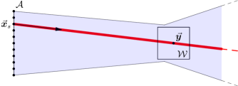
Figure 4. Given an array $\mathcal{A}$ and a region $\mathcal{W}$ containing the scatterers to image, assumption 5.1 ensures the receiver location $\vec{\bm{x}}_{r}$ is outside of the blue shaded region. This guarantees the Kirchhoff images using data $\bm{p}$ and the recovered $\bm{p}+\zeta\bm{g}_{0}$ are essentially the same. The positive ray in the direction $\vec{\bm{x}}_{s}-\vec{\bm{y}}$ for particular $\vec{\bm{x}}_{s}\in\mathcal{A}$ and $\vec{\bm{y}}\in\mathcal{W}$ is indicated in red. If $\vec{\bm{x}}_{r}$ is outside the blue shaded region, we have $(\vec{\bm{x}}_{s}-\vec{\bm{x}}_{r})/|\vec{\bm{x}}_{s}-\vec{\bm{x}}_{r}|\neq(\vec{\bm{x}}_{s}-\vec{\bm{y}})/|\vec{\bm{x}}_{s}-\vec{\bm{y}}|$ for all $\vec{\bm{x}}_{s}\in\mathcal{A}$ and all $\vec{\bm{y}}\in\mathcal{W}$.

Theorem 5.2.

Provided assumption 5.1 holds, the image of the reconstructed array response vector is

$$\Gamma_{\text{KM}}[\bm{p}+\zeta\bm{g}_{0},\omega](\vec{\bm{y}})\approx\Gamma_{\text{KM}}[\bm{p},\omega](\vec{\bm{y}}).$$

Proof.

First we approximate the Kirchhoff imaging functional (7) by an integral over the array $\mathcal{A}$, i.e.

(23) $$\Gamma_{\text{KM}}[\zeta\bm{g}_{0},\omega](\vec{\bm{y}}) =\overline{\widehat{G}}(\vec{\bm{x}}_{r},\vec{\bm{y}},\omega)\bm{g}_{0}(\vec{\bm{y}},\omega)^{*}\zeta(\vec{\bm{x}}_{r},\omega)\bm{g}_{0}(\vec{\bm{x}}_{r},\omega)$$

$$\sim\zeta(\vec{\bm{x}}_{r},\omega)\int_{\mathcal{A}}d\bm{x}_{s}C(\bm{x}_{s})\exp\left(\imath\omega c_{0}^{-1}\big{(}|\vec{\bm{x}}_{s}-\vec{\bm{x}}_{r}|-|\vec{\bm{x}}_{s}-\vec{\bm{y}}|-|\vec{\bm{y}}-\vec{\bm{x}}_{r}|\big{)}\right),$$

where the symbol $\sim$ means equal up to a constant and $C(\bm{x}_{s})$ collects smooth geometric spreading terms.

Let us first use the stationary phase method (see e.g. [1]) on the integral over $\mathcal{A}$. In the high frequency limit $\omega\to\infty$, the dominant contribution comes from stationary points of the phase, i.e. the points $\vec{\bm{x}}_{s}$ for which

$$\nabla_{\vec{\bm{x}}_{s}}\Big{(}|\vec{\bm{x}}_{s}-\vec{\bm{x}}_{r}|-|\vec{\bm{x}}_{s}-\vec{\bm{y}}|-|\vec{\bm{y}}-\vec{\bm{x}}_{r}|\Big{)}=0.$$

The stationary points must then satisfy

$$\frac{\vec{\bm{x}}_{s}-\vec{\bm{x}}_{r}}{|\vec{\bm{x}}_{s}-\vec{\bm{x}}_{r}|}=\frac{\vec{\bm{x}}_{s}-\vec{\bm{y}}}{|\vec{\bm{x}}_{s}-\vec{\bm{y}}|}.$$

Thus by assumption 5.1, there are no stationary points in the phase of the integral over the array $\mathcal{A}$ appearing in (23). Neglecting boundary effects, this integral goes to zero faster than any polynomial in $\omega$ (see e.g. [2]).

We now show that in the high frequency limit $\omega\to\infty$, we have $\zeta(\vec{\bm{x}}_{r},\omega)\to 1/2$. Recalling (21), we have

(24) $$\zeta(\vec{\bm{x}}_{r},\omega) =\frac{1}{2}+\frac{\bm{g}_{0}(\vec{\bm{x}}_{r},\omega)^{*}\bm{p}(\vec{\bm{x}}_{r},\omega)-\bm{p}(\vec{\bm{x}}_{r},\omega)^{*}\bm{g}_{0}(\vec{\bm{x}}_{r},\omega)}{\bm{g}_{0}(\vec{\bm{x}}_{r},\omega)^{*}\bm{g}_{0}(\vec{\bm{x}}_{r},\omega)}$$

$$\sim\frac{1}{2}+\frac{\omega^{2}}{c_{0}^{2}}\int d\vec{\bm{z}}\int_{\mathcal{A}}d\bm{x}_{s}C(\bm{x}_{s})\exp\left(\imath\omega c_{0}^{-1}\big{(}|\vec{\bm{x}}_{s}-\vec{\bm{z}}|+|\vec{\bm{z}}-\vec{\bm{x}}_{r}|-|\vec{\bm{x}}_{s}-\vec{\bm{x}}_{r}|\big{)}\right)$$

$$\qquad-\frac{\omega^{2}}{c_{0}^{2}}\int d\vec{\bm{z}}\int_{\mathcal{A}}d\bm{x}_{s}C(\bm{x}_{s})\exp\left(\imath\omega c_{0}^{-1}\big{(}|\vec{\bm{x}}_{s}-\vec{\bm{x}}_{r}|-|\vec{\bm{x}}_{s}-\vec{\bm{z}}|-|\vec{\bm{z}}-\vec{\bm{x}}_{r}|\big{)}\right),$$

where $C(\vec{\bm{x}}_{s})$ collects geometric spreading terms and $|\bm{g}_{0}(\vec{\bm{x}}_{r},\omega)|^{-2}$, which is actually independent of the frequency $\omega$. By assumption 5.1, the integrals over $\mathcal{A}$ in (24) do not have any stationary points. Thus if we neglect boundary terms, these integrals must go to zero faster than any polynomial in $\omega$ (see e.g. [2]), meaning that $\zeta(\vec{\bm{x}}_{r},\omega)\to 1/2$ as $\omega\to\infty$. Thus $\Gamma_{\text{KM}}[\zeta\bm{g}_{0},\omega](\vec{\bm{y}})\to 0$ as $\omega\to\infty$. ∎

6. Autocorrelation measurements

Up to this point we have assumed deterministic control over the source illuminations. In this section we relax this control by driving the array with stochastic signals. We start in section 6.1 by recalling an ergodicity result of Garnier and Papanicolaou [10] which guarantees that if Gaussian stochastic processes are used to drive the sources, the realization average of the total field can be well approximated by time averages of the total field. Then in section 6.2 we adapt the source pair illumination strategy to pairs of sources driven by two correlated Gaussian processes, with (known) correlation identical for different pairs. From these pairwise illuminations we measure empirical autocorrelations to obtain intensity measurements that are essentially (up to ergodic averaging) the same as those using the deterministic strategy of section 3.1.

6.1. Stochastic array illuminations

We consider array illuminations $\bm{f}(t)\in\mathbb{C}^{N}$ given by a stationary Gaussian process with mean zero and with correlation the $N\times N$ matrix function

(25) $$\mathsf{R}(\tau)=\langle\overline{\bm{f}}(t)\bm{f}^{\mathsf{T}}(t+\tau)\rangle.$$

Here $\langle\cdot\rangle$ denotes the expectation with respect to realizations of $\bm{f}$, and in an abuse of notation we have denoted by $\bm{f}(t)$ the time domain vector of signals driving the array. Since $R_{s,s^{\prime}}(\tau)=\langle\overline{f}_{s}(t)f_{s^{\prime}}(t+\tau)\rangle=\overline{\langle\overline{f}_{s^{\prime}}(t+\tau)f_{s}(t)\rangle}=\overline{R_{s^{\prime},s}(-\tau)}$ for $s,s^{\prime}=1,\ldots,N$, we have $\mathsf{R}(\tau)=\mathsf{R}^{*}(-\tau)$ and so $\widehat{\mathsf{R}}(\omega)$ is a Hermitian $N\times N$ matrix.

The total field $u$ at the receiver arising from the array illumination $\bm{f}$ is, in the time domain,

(26) $$u(\vec{\bm{x}}_{r},t)=\sum_{s=1}^{N}\int dt^{\prime}G(\vec{\bm{x}}_{r},\vec{\bm{x}}_{s},t-t^{\prime})f_{s}(t^{\prime}),$$

where $G$ is the Born approximation of the inhomogeneous Green function, i.e.

$$G(\vec{\bm{x}}_{r},\vec{\bm{x}}_{s},t)=\frac{1}{2\pi}\int d\omega e^{-\imath\omega t}\Big{[}\widehat{G}_{0}(\vec{\bm{x}}_{r},\vec{\bm{x}}_{s},\omega)+k^{2}\int d\vec{\bm{z}}\rho(\vec{\bm{z}})\widehat{G}_{0}(\vec{\bm{x}}_{r},\vec{\bm{z}},\omega)\widehat{G}_{0}(\vec{\bm{z}},\vec{\bm{x}}_{s},\omega)\Big{]}.$$

The empirical autocorrelation of $u$ is

(27) $$\psi(\vec{\bm{x}}_{r},\tau)=\frac{1}{2T}\int_{-T}^{T}\overline{u}(\vec{\bm{x}}_{r},t)u(\vec{\bm{x}}_{r},t+\tau)dt,$$

where $T$ is a known measurement time. Following Garnier and Papanicolaou [10], we formulate proposition 6.1 regarding the statistical stability and ergodicity of (27). This proposition is essentially the same as [10, Proposition 4.1], but we make small modifications to allow for complex fields and more general correlations in space. We include it here for the sake of completeness and the proof can be found in appendix A.

Proposition 6.1.

Assume $\bm{f}$ satisfies (25). The expectation (w.r.t. realizations of $\bm{f}$) of the empirical autocorrelation (27) is independent of measurement time $T$:

(28) $$\langle\psi(\vec{\bm{x}}_{r},\tau)\rangle=\Psi(\vec{\bm{x}}_{r},\tau),$$

where

(29) $$\Psi(\vec{\bm{x}}_{r},\tau) =\sum_{s,s^{\prime}=1}^{N}\int dt^{\prime}\int dt^{\prime\prime}\overline{G}(\vec{\bm{x}}_{r},\vec{\bm{x}}_{r},-t^{\prime})G(\vec{\bm{x}}_{r},\vec{\bm{x}}_{s^{\prime}},\tau-t^{\prime\prime})R_{s,s^{\prime}}(t^{\prime\prime}-t^{\prime})$$

$$=\frac{1}{2\pi}\int d\omega e^{-\imath\omega\tau}\bm{g}(\vec{\bm{x}}_{r},\omega)^{*}\widehat{\mathsf{R}}(\omega)\bm{g}(\vec{\bm{x}}_{r},\omega).$$

Furthermore, (27) is ergodic, i.e.

(30) $$\psi(\vec{\bm{x}}_{r},\tau)\xrightarrow{T\to\infty}\Psi(\vec{\bm{x}}_{r},\tau).$$

6.2. Pairwise stochastic illuminations

We make $N_{p}$ illuminations each corresponding to using only two distinct sources $(i(m),j(m))\in\{1,\ldots,N\}^{2}$, $m=1,\ldots,N_{p}$. The correlation matrix for the $m-$th experiment has the form

(31) $$\widehat{\mathsf{R}}_{m}(\omega)=\mathsf{F}_{m}\mathsf{C}(\omega)\mathsf{F}_{m}^{\mathsf{T}},$$

where $\mathsf{F}_{m}=[\bm{e}_{i(m)},\bm{e}_{j(m)}]\in\mathbb{R}^{N\times 2}$ and $\mathsf{C}(\omega)$ is a known $2\times 2$ Hermitian positive semidefinite matrix that represents the correlation between the two sources and is assumed to be the same for all experiments. For instance, if we send the same signal with power spectrum $F(\omega)$ from both sources in a pair, this correlation matrix is

$$\mathsf{C}(\omega)=F(\omega)\begin{bmatrix}1&1\\ 1&1\end{bmatrix}.$$

By the ergodicity (30) of proposition 6.1, when we measure the empirical autocorrelation $\psi_{m}$ of $u_{m}$ at the receiver $\vec{\bm{x}}_{r}$ for long enough time $T$, the empirical autocorrelation is close to an intensity measurement, i.e.

(32) $$\widehat{\Psi}_{m}(\vec{\bm{x}}_{r},\omega)=\bm{g}(\vec{\bm{x}}_{r},\omega)^{*}\mathsf{F}_{m}\mathsf{C}(\omega)\mathsf{F}_{m}^{\mathsf{T}}\bm{g}(\vec{\bm{x}}_{r},\omega).$$

By using appropriate single source illuminations driven by a signal with known correlation, it is possible to measure

(33) $$\widehat{\Psi}_{i}^{0}(\vec{\bm{x}}_{r},\omega)=\bm{g}^{*}(\vec{\bm{x}}_{r},\omega)\bm{e}_{i}\bm{e}_{i}^{\mathsf{T}}\bm{g}(\vec{\bm{x}}_{r},\omega).~{}\text{ for $i=1,\ldots,N$.}$$

From (32) and (33) we obtain the $m-$th measurement

(34) $$d_{m}(\vec{\bm{x}}_{r},\omega) =\widehat{\Psi}_{m}(\vec{\bm{x}}_{r},\omega)-C_{11}(\omega)\widehat{\Psi}_{i(m)}^{0}(\vec{\bm{x}}_{r},\omega)-C_{22}(\omega)\widehat{\Psi}_{j(m)}^{0}(\vec{\bm{x}}_{r},\omega)$$

$$=\bm{g}(\vec{\bm{x}}_{r},\omega)^{*}\mathsf{F}_{m}\mathsf{D}(\omega)\mathsf{F}_{m}^{\mathsf{T}}\bm{g}(\vec{\bm{x}}_{r},\omega),$$

where the matrix $\mathsf{D}$ is $2\times 2$, Hermitian with zero diagonal, i.e. precisely of the same form as the matrix $\mathsf{D}$ we encountered in the intensity measurements case (11).

Proceeding analogously as in section 3.1 and recalling that $\bm{g}=\bm{g}_{0}+\bm{p}$ we have

$$d_{m}(\vec{\bm{x}}_{r},\omega) =\big{(}\bm{g}_{0}+\bm{p}\big{)}^{*}\mathsf{F}_{m}\mathsf{D}(\omega)\mathsf{F}_{m}^{\mathsf{T}}(\bm{g}_{0}+\bm{p}\big{)}.$$

Collecting the measurements for $m=1,\ldots,N_{p}$ and neglecting the quadratic term in $\bm{p}$ we have the approximate data

(35) $$\begin{bmatrix}d_{1}(\vec{\bm{x}}_{r},\omega)\\ d_{2}(\vec{\bm{x}}_{r},\omega)\\ \vdots\\ d_{N_{p}}(\vec{\bm{x}}_{r},\omega)\end{bmatrix}\approx\bm{d}(\vec{\bm{x}}_{r},\omega)=\mathsf{M}(\vec{\bm{x}}_{r},\omega)\begin{bmatrix}\text{Re}\big{(}\bm{g}_{0}+2\bm{p}\big{)}\\ \text{Im}\big{(}\bm{g}_{0}+2\bm{p}\big{)}\end{bmatrix},$$

where the matrix $\mathsf{M}\in\mathbb{R}^{N_{p}\times 2N}$ is again given by (13). Thus, the data (35) obtained by measuring the empirical autocorrelation (27) and using correlated pair illuminations, is essentially the same as the data obtained using deterministic source pairs (12). Hence the analysis of the matrix $\mathsf{M}$ of §4 holds and we can use Kirchhoff migration as we did in §5 for the intensity measurements case.

Remark 6.2 (Uncorrelated background illumination).

The proposed illumination strategy is robust with respect to noise and even allows to send the same Gaussian signal from the $m-$th source pair $(i(m),j(m))$ and independent Gaussian signals from all remaining sources on the array. If the independent signals have the same spectral density $F(\omega)$ as the source pair signal, the correlation matrix for the $m-$th experiment is

(36) $$\widehat{\mathsf{R}}_{m}(\omega)=F(\omega)\left(\mathsf{I}+\mathsf{F}_{m}\begin{bmatrix}0&1\\ 1&0\end{bmatrix}\mathsf{F}_{m}^{\mathsf{T}}\right),$$

where $\mathsf{I}$ is $N\times N$ identity matrix. By subtracting from the autocorrelation for the $m-$th experiment, the autocorrelation for a reference illumination that sends independent Gaussian signals with correlation matrix $F(\omega)\mathsf{I}$, it is possible to obtain $m-$th measurement (34) with

$$\mathsf{D}(\omega)=F(\omega)\begin{bmatrix}0&1\\ 1&0\end{bmatrix}.$$

7. Additive noise

Here we discuss the effects of additive instrumental noise in autocorrelated measurements of the total field. The total field at $\vec{\bm{x}}_{r}$ resulting from illuminating with the $m-$th pair and tainted with additive noise is $u_{m}(\vec{\bm{x}}_{r},t)+\xi(t)$. We assume the noise $\xi$ is a stationary Gaussian process with mean zero and spectral density

(37) $$\widehat{\Xi}(\omega)=\exp\left(\frac{-l_{c}^{2}(\omega-\omega_{0})^{2}}{4\pi}\right).$$

Here $l_{c}$ represents the correlation time of the noise (i.e. $\Xi(\tau)=\langle\overline{\xi}(t)\xi(t+\tau)\rangle\approx 0$ for $\tau\gg l_{c}$) and $\omega_{0}$ is the central angular frequency of the noise. If the noise $\xi$ is independent of the signals used to drive the source pairs, it can be shown using the techniques of appendix A that

$$\frac{1}{2T}\int_{-T}^{T}dt\big{(}\overline{u}_{m}(\vec{\bm{x}}_{r},t)+\overline{\xi}(t)\big{)}\big{(}u_{m}(\vec{\bm{x}}_{r},t+\tau)+\xi(t+\tau)\big{)}\xrightarrow{T\to\infty}\Psi_{m}(\vec{\bm{x}}_{r},\tau)+\Xi(\tau),$$

where $\Psi_{m}$ is given by (29).

Assuming the same form of instrumental noise in the single source reference measurements, the $m-$th measurement $d_{m}(\vec{\bm{x}}_{r},\omega)$ is

$$d_{m}(\vec{\bm{x}}_{r},\omega)=\big{(}\bm{g}_{0}+\bm{p}\big{)}^{*}\mathsf{F}_{m}\mathsf{D}(\omega)\mathsf{F}_{m}^{\mathsf{T}}\big{(}\bm{g}_{0}+\bm{p}\big{)}+C\widehat{\Xi}(\omega).$$

for some $C\in\mathbb{R}$. Neglecting the terms which are quadratic in $\bm{p}$ and going back to the time domain we have

$$d_{m}(\vec{\bm{x}}_{r},\tau)\approx\frac{1}{2\pi}\int d\omega e^{-\imath\omega\tau}\Big{[} \bm{g}_{0}(\vec{\bm{x}}_{r},\omega)^{*}\mathsf{F}_{m}\mathsf{D}(\omega)\mathsf{F}_{m}^{\mathsf{T}}\bm{g}_{0}(\vec{\bm{x}}_{r},\omega)$$

$$+ \bm{g}_{0}(\vec{\bm{x}}_{r},\omega)^{*}\mathsf{F}_{m}\mathsf{D}(\omega)\mathsf{F}_{m}^{\mathsf{T}}\bm{p}(\vec{\bm{x}}_{r},\omega)$$

$$+ \bm{p}(\vec{\bm{x}}_{r},\omega)^{*}\mathsf{F}_{m}\mathsf{D}(\omega)\mathsf{F}_{m}^{\mathsf{T}}\bm{g}_{0}(\vec{\bm{x}}_{r},\omega)\Big{]}+C\Xi(\tau),$$

with the slight abuse of notation of using $d_{m}$ for both time and frequency domain quantities. The second and third terms in the integrand are incident-scattered field correlations and contain the available information about the scattering potential $\rho(\vec{\bm{y}})$.

For simplicity, we now focus on the case where the source pair signals have correlation matrix

$$\mathsf{D}(\omega)=F(\omega)\begin{bmatrix}0&e^{\imath\omega\phi}\\ e^{-\imath\omega\phi}&0\end{bmatrix}.$$

Such correlation corresponds to sending a signal from one of the sources in a pair and a copy of the same signal delayed by $\phi$ from the other source. For a point scatterer at $\vec{\bm{y}}$, the incident-scattered terms have peaks at delay times $\tau(\vec{\bm{y}})$ corresponding to differences between travel times of a reflected path and direct path, i.e. for the $m-$th experiment the peaks occur at the four possible delays

$$\tau(\vec{\bm{y}})=\begin{cases}\pm((|\vec{\bm{x}}_{j(m)}-\vec{\bm{y}}|+|\vec{\bm{y}}-\vec{\bm{x}}_{r}|-|\vec{\bm{x}}_{i(m)}-\vec{\bm{x}}_{r}|)/c_{0}+\phi),\\ \pm((|\vec{\bm{x}}_{i(m)}-\vec{\bm{y}}|+|\vec{\bm{y}}-\vec{\bm{x}}_{r}|-|\vec{\bm{x}}_{j(m)}-\vec{\bm{x}}_{r}|)/c_{0}-\phi).\end{cases}$$

Consider then the minimal delay time $\tau_{\min}(\vec{\bm{y}})$ given by

(38) $$\tau_{\min}(\vec{\bm{y}})=\min_{\vec{\bm{x}}_{s},\vec{\bm{x}}_{s^{\prime}}\in\mathcal{A}}\left|\frac{|\vec{\bm{x}}_{s}-\vec{\bm{y}}|+|\vec{\bm{y}}-\vec{\bm{x}}_{r}|-|\vec{\bm{x}}_{s^{\prime}}-\vec{\bm{x}}_{r}|}{c_{0}}\pm\phi\right|,$$

that is the minimal delay time we expect the incident-scattered correlations to peak. If we assume the additive noise decorrelates much faster than the first incident-scattered arrival from $\vec{\bm{y}}$ (i.e. $l_{c}\ll\tau_{\min}(\vec{\bm{y}})$), then the information of the scatterer $\rho(\vec{\bm{y}})$ contained in $d_{m}(\vec{\bm{x}}_{r},\tau)$ is essentially unchanged (up to ergodic averaging). Hence we can stably image using the proposed method at $\vec{\bm{y}}$ provided $\tau_{\min}(\vec{\bm{y}})\gg l_{c}$.

8. Numerical experiments

Here we include 2D numerical experiments of our proposed imaging routine for scalings corresponding to acoustics (§8.1) and optics (§8.2). We demonstrate the stochastic source pair illumination strategy for the acoustic regime, i.e. we compute the autocorrelations for time domain data. In the optic regime this is an expensive calculation, so we use instead power spectra (i.e. deterministic illuminations).

8.1. Acoustic regime

For imaging in an acoustic regime, our choice of physical parameters corresponds to ultrasound in water. We choose the background wave velocity to be $c_{0}=1500$ m/s. The central frequency for all signals (sources and additive noise) is $3$ MHz, which gives a central wavelength of $\lambda_{0}=0.5$ mm. We center a source array $\mathcal{A}$ at the origin consisting of $41$ sources at coordinates $\vec{\bm{x}}_{s}=(0,-10\lambda_{0}+(s-1)\lambda_{0}/2)$ for $s=1,\ldots,41$. A single receiver is located at the coordinate $\vec{\bm{x}}_{r}=(-20\lambda_{0},-20\lambda_{0})$ (see figure 1).

We generate a stationary Gaussian time signal $f(t)$ with mean zero and correlation function

$$F(\tau)=\exp\left(-\pi\frac{\tau^{2}}{t_{c}^{2}}\right),$$

using the Wiener-Khinchin theorem. The correlation time $t_{c}\approx 1.25$ $\mu$s which gives the signal an effective frequency band $[1,5]$ MHz. We generate time signals of length $2T$ for $T\approx 260$ $\mu$s with $8001$ uniformly spaced samples. This sampling is enough to resolve the frequencies in the angular frequency band $\mathcal{B}$, while $T$ is sufficient to observe ergodic averaging (see §6). By placing the same realization of this signal $\widehat{f}(\omega)$ at the locations $\vec{\bm{x}}_{i(m)}$ and $\vec{\bm{x}}_{j(m)}$ we generate the pair illumination $\bm{f}_{m}(\omega)=\widehat{f}(\omega)(\bm{e}_{i(m)}+\bm{e}_{j(m)}).$ Similarly, by placing an independent realization of $\widehat{f}(\omega)$ at location $\vec{\bm{x}}_{i}$ we generate the single source reference illumination $\bm{f}_{i}^{0}(\omega)=\widehat{f}(\omega)\bm{e}_{i}$.

For all experiments, synthetic data is generated in the frequency domain using the Born approximation. We assume 3D wave propagation for simplicity so that $G_{0}$ is given by (3) for $d=3$. The $m-$th measurement is obtained through the formula

$$d_{m}(\vec{\bm{x}}_{r},\omega)=\widehat{\Psi}_{m}(\vec{\bm{x}}_{r},\omega)-\widehat{\Psi}_{i(m)}^{0}(\vec{\bm{x}}_{r},\omega)-\widehat{\Psi}_{j(m)}^{0}(\vec{\bm{x}}_{r},\omega),$$

where

$$\widehat{\Psi}_{m}(\vec{\bm{x}}_{r},\omega) =\Big{|}\big{(}\bm{g}_{0}(\vec{\bm{x}}_{r},\omega)+\bm{p}(\vec{\bm{x}}_{r},\omega)\big{)}^{\mathsf{T}}\bm{f}_{m}(\omega)\Big{|}^{2},$$

$$\widehat{\Psi}_{i}^{0}(\vec{\bm{x}}_{r},\omega) =\Big{|}\big{(}\bm{g}_{0}(\vec{\bm{x}}_{r},\omega)+\bm{p}(\vec{\bm{x}}_{r},\omega)\big{)}^{\mathsf{T}}\bm{f}_{i}^{0}(\omega)\Big{|}^{2},$$

with $\bm{g}_{0}$ and $\bm{p}$ defined by (2) and (6) respectively.

For these simulations we use the full set of pair illuminations, which for $N=41$ source locations, generates a measurement matrix $\mathsf{M}(\vec{\bm{x}}_{r},\omega)\in\mathbb{R}^{820\times 82}$. We use the Moore Penrose pseudoinverse $\mathsf{M}^{\dagger}$ to recover $\bm{p}+\zeta\bm{g}_{0}$ for each $\omega\in\mathcal{B}$. When the number of sources $N$ and thus the dimension of $\mathsf{M}$ is large (recall $\mathsf{M}\in\mathbb{R}^{N(N-1)/2\times N}$), the pseudoinverse could become computationally expensive. However, the system is sparse as it contains only $4$ non-zero elements per row, so linear least square solvers that exploit sparsity (e.g. CGLS [17]) may be more efficient than our approach. Furthermore, as discussed in §4 we can reduce the size of $\mathsf{M}$ to $2N\times 2N$ while keeping the nullspace of $\mathsf{M}$ one-dimensional by using an appropriate subset of source pairs.

We form an image at $\vec{\bm{y}}\in\mathcal{W}=\{(100\lambda_{0}+i\lambda_{0}/2.5,j\lambda_{0}/2.5),\text{ for }i,j=-25,\ldots,25\}$ using the Kirchhoff migration functional (§2.2), summed over the bandwidth band $\mathcal{B}$,

$$\Gamma_{\text{KM}}[\bm{p}+\zeta\bm{g}_{0}](\vec{\bm{y}})=\int_{\mathcal{B}}d\omega\Gamma_{\text{KM}}[\bm{p}+\zeta\bm{g}_{0},\omega](\vec{\bm{y}}).$$

For our first experiment, we place a single point reflector at the location $\vec{\bm{y}}=(100\lambda_{0},0)$, with refractive index perturbation $\rho(\vec{\bm{y}})=1\times 10^{-8}$. The migrated image (figure 5a) indeed exhibits the cross-range (Rayleigh) resolution estimate $\lambda_{0}L/a\approx 5\lambda_{0}$ and range resolution estimate $c_{0}/|\mathcal{B}|\approx 1\lambda_{0}$. Note that there is a trade-off in the choice of the reflectivity: $\rho$ has to be sufficiently small so that the quadratic terms in $\bm{p}$ can be neglected in (12). However the smaller $\rho$ is, the longer the acquisition time $T$ has to be in order to better observe the reflected-incident correlations in the data.

In our second experiment (figure 5b), we consider two oblique reflectors located at $\vec{\bm{y}}_{1}=(99\lambda_{0},-2\lambda_{0})$ and $\vec{\bm{y}}_{2}=(103\lambda_{0},4\lambda_{0})$ each with $\rho(\vec{\bm{y}}_{i})=1\times 10^{-8}$. We include a reconstruction of an extended scatterer (line segment) in figure 6. Here the line segment is generated as a set of point reflectors each with $\rho(\vec{\bm{y}}_{i})=1\times 10^{-9}$ uniformly spaced by $\lambda_{0}/8$.

$\Gamma_{\text{KM}}[\bm{p}](\vec{\bm{y}})$

$\Gamma_{\text{KM}}[\bm{p}+\zeta\bm{g}_{0}](\vec{\bm{y}})$

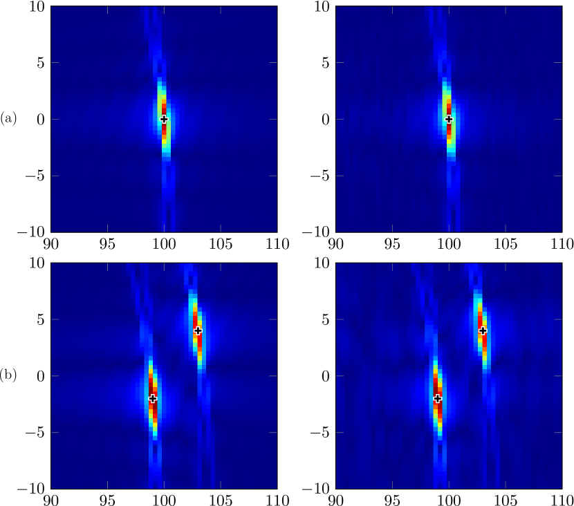
Figure 5. Kirchhoff images of (a) one point and (b) two point reflectors, whose true positions are indicated with crosses. The left column uses the full waveform data $\bm{p}$, while the right column use the recovered data $\bm{p}+\zeta\bm{g}_{0}$. The horizontal and vertical axes display the range and cross-range respectively, with scales in central wavelengths $\lambda_{0}$.

$\Gamma_{\text{KM}}[\bm{p}](\vec{\bm{y}})$

$\Gamma_{\text{KM}}[\bm{p}+\zeta\bm{g}_{0}](\vec{\bm{y}})$

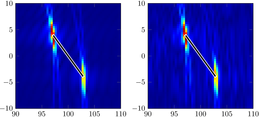
Figure 6. Kirchhoff images of an extended reflector. The left column uses the full waveform data $\bm{p}$, while the right column use the recovered data $\bm{p}+\zeta\bm{g}_{0}$. The horizontal and vertical axes display the range and cross-range respectively, with scales in central wavelengths $\lambda_{0}$.

We now demonstrate the robustness of the proposed method with respect to additive noise (see section 7). Here we have taken a realization of the data for a single point reflector (c.f. figure 5a) and perturbed each measurement with additive noise as follows. The $m-$th signal $\widehat{u}_{m}(\vec{\bm{x}}_{r},\omega)$ has total power $p_{m}=\int|\widehat{u}_{m}(\vec{\bm{x}}_{r},\omega)|^{2}d\omega$. We construct a Gaussian signal $\xi_{m}(t)$ with mean zero, spectral density (37), $l_{c}\approx 1.25$ $\mu$s and total power $1$. This allows to obtain the perturbed total field $\widehat{u}_{m}(\vec{\bm{x}}_{r},\omega)+\sqrt{\nu p_{m}}\widehat{\xi}_{m}(\omega)$ for some $\nu>0$. The $m-$th measurement with additive noise is thus $d_{m}(\vec{\bm{x}}_{r},\omega)=|\widehat{u}_{m}(\vec{\bm{x}}_{r},\omega)|^{2}+\nu p_{m}|\widehat{\xi}(\omega)|^{2}$. Thus the ratio of the signal power to the noise power is $1/\nu$. The signal-to-noise ratio (SNR) is then

$$\text{SNR}_{m}=-10\log_{10}(\nu)\text{dB}.$$

Figure 7 shows the reconstruction from data with SNR${}_{m}=0$ dB for each $m$, meaning that the signal and the noise have the same power.

$\Gamma_{\text{KM}}[\bm{p}](\vec{\bm{y}})$

$\Gamma_{\text{KM}}[\bm{p}+\zeta\bm{g}_{0}](\vec{\bm{y}})$

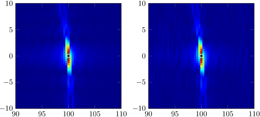
Figure 7. Additive noise: (left) array response vector migration $\Gamma_{\text{KM}}[\bm{p}](\vec{\bm{y}})$, (right) recovered array response vector migration $\Gamma_{\text{KM}}[\bm{p}+\zeta\bm{g}_{0}](\vec{\bm{y}})$ for SNR${}_{m}=0$dB. The horizontal and vertical axes display the range and cross-range respectively measured in central wavelengths $\lambda_{0}$.

Lastly we perform an experiment that sends as the $m-$th illumination the usual correlated pair illumination $\bm{f}_{m}$, and uncorrelated noise from the remaining sources on the array $\mathcal{A}$ (see remark 6.2). To generate this illumination we place the same realization of the signal $\widehat{f}(\omega)$ at the locations $\bm{x}_{i(m)}$ and $\bm{x}_{j(m)}$, and independent realizations of $\widehat{f}(\omega)$ at the remaining source locations. Similarly, a reference illumination is generated by placing independent realizations of $\widehat{f}(\omega)$ at all locations on the array $\mathcal{A}$. By measuring the autocorrelation of the resulting fields we obtain data that is essentially the same form as $d_{m}(\vec{\bm{x}}_{r},\omega)$. Figure 8 shows this experiment with the single point reflector located at $\vec{\bm{y}}=(100\lambda_{0},0)$ and reflectivity $\rho(\vec{\bm{y}})=1\times 10^{-8}$.

$\Gamma_{\text{KM}}[\bm{p}](\vec{\bm{y}})$

$\Gamma_{\text{KM}}[\bm{p}+\zeta\bm{g}_{0}](\vec{\bm{y}})$

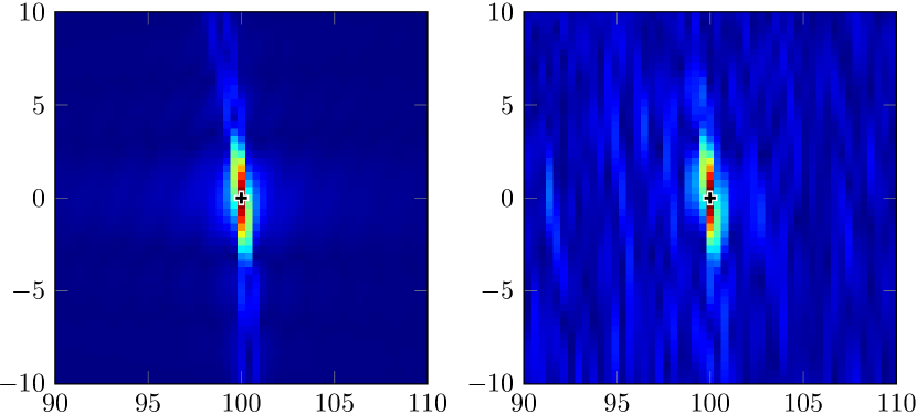
Figure 8. Uncorrelated background illumination: (left) array response vector migration $\Gamma_{\text{KM}}[\bm{p}](\vec{\bm{y}})$, (b) recovered array response vector migration $\Gamma_{\text{KM}}[\bm{p}+\zeta\bm{g}_{0}](\vec{\bm{y}})$ for SNR${}_{m}=0$dB. The horizontal and vertical axes display the range and cross-range respectively measured in central wavelengths $\lambda_{0}$.

8.2. Optic regime

For imaging in an optic regime, we use the background wave velocity $c_{0}=3\times 10^{8}$ m/s and central frequency $\approx 589$ THz which gives a central wavelength $\lambda_{0}\approx 509$ nm. Our source array $\mathcal{A}$ is again centered at the origin, but now consists of $1001$ sources located at coordinates $\vec{\bm{x}}_{s}=(0,-500\lambda_{0}+(s-1)\lambda_{0})$ for $s=1,\ldots,1001$, and we set $\vec{\bm{x}}_{r}=(-1000\lambda_{0},-1000\lambda_{0})$.

We generate intensity data $\bm{d}(\vec{\bm{x}}_{r},\omega)$ as

$$d_{m}(\bm{x}_{r},\omega)=\Big{|}\big{(}\bm{g}_{0}+\bm{p}\big{)}^{T}(\bm{e}_{i(m)}+\bm{e}_{j(m)})\Big{|}^{2}-\Big{|}\big{(}\bm{g}_{0}+\bm{p}\big{)}^{T}\bm{e}_{i(m)}\Big{|}^{2}-\Big{|}\big{(}\bm{g}_{0}+\bm{p}\big{)}^{T}\bm{e}_{j(m)}\Big{|}^{2},$$

for $100$ (angular) frequencies $\omega$ uniformly spaced in the frequency band $[429,750]$ THz. This corresponds to performing the source pair experiments (source pair illuminations and single source reference illuminations) for $100$ different monochromatic visible light sources with wavelengths $\lambda\in[400,700]$ nm, equally spaced in frequency. Since there are a large number of sources in this setup ($N=1001$), we implement the strategy discussed in §4 to reduce the number of source pair experiments from $N_{p}=N(N-1)/2$ to $N_{p}=2N$.

As before, we use the pseudoinverse $\mathsf{M}^{\dagger}$ to recover $\bm{p}+\zeta\bm{g}_{0}$ for each frequency $\omega\in\mathcal{B}$, and then use the Kirchhoff migration functional (§2.2) to form an image. Here we use the image window $\mathcal{W}=\{(5000\lambda_{0}+i\lambda_{0}/2.5,j\lambda_{0}/2.5),\text{for $i,j=-25,\ldots,25$}\}$. In figure 9(b) we demonstrate the migrated image for two point reflectors placed at $\vec{\bm{y}}_{1}=(4098\lambda_{0},3\lambda_{0})$ and $\vec{\bm{y}}_{2}=(5004\lambda_{0},-5\lambda_{0})$ each with reflectivity $\rho(\vec{\bm{y}}_{i})=1\times 10^{-17}$. Although we are significantly undersampling the data in frequency and the source spacing is larger than $\lambda_{0}/2$, the spot sizes still exhibit the Kirchhoff migration resolution estimates (§2.2) of $\lambda_{0}L/a\approx 5\lambda_{0}$ in cross-range and $c_{0}/|\mathcal{B}|\approx 2\lambda_{0}$ in range.

$\Gamma_{\text{KM}}[\bm{p}](\vec{\bm{y}})$

$\Gamma_{\text{KM}}[\bm{p}+\zeta\bm{g}_{0}](\vec{\bm{y}})$

Figure 9. Optic regime:(left) array response vector migration $\Gamma_{\text{KM}}[\bm{p}](\vec{\bm{y}})$, (b) recovered array response vector migration $\Gamma_{\text{KM}}[\bm{p}+\zeta\bm{g}_{0}](\vec{\bm{y}})$. The horizontal and vertical axes display the range and cross-range respectively measured in central wavelengths $\lambda_{0}$.

9. Discussion

By sending correlated signals from different pairs of locations we have shown that from intensity data we can recover full waveform data by solving a linear system. This linear system has a known one-dimensional nullspace provided the sources and receiver satisfy the distance conditions given by assumption 4.1, which allows for the recovery of $\bm{p}+\zeta\bm{g}_{0}$. We show this quantity is enough to use standard migration techniques (e.g. Kirchhoff migration $\Gamma_{\text{KM}}$) provided the sources and receiver satisfy the additional geometric conditions of assumption 5.1. Thus we obtain full waveform resolution estimates for an image formed from intensity-only data.

Our method relies only on knowledge of paired source locations and the correlation of the signals being sent. This allows us to relax illumination control by using paired stochastic signals. By measuring autocorrelations of the resulting fields, we obtain essentially the same intensity data as with using deterministic source pairs. These stochastic illuminations can be created e.g. by using a configurable mask that is parallel to the wave fronts of an incoherent plane wave.

The linear system we solve has size $2N\times 2N$ and is very sparse (up to 4 non-zero entries per row). In our simulations we used $\mathsf{M}^{\dagger}$, however sparse solvers such as CGLS (see e.g. [17]) could be used. To form the system we need at least $3N$ different illuminations, $2N$ pair illuminations plus $N$ reference illuminations. However, in our illumination strategy, the phase of the source signals does not need to be known. We replace the direct phase control by the natural phase modulation that comes from the different positions of the signals.

We use the geometric imaging conditions (assumption 5.1) to show the nullspace of $\mathsf{M}$ does not affect imaging via $\Gamma_{\text{KM}}$. This assumption imposes some restrictions on the juxtaposition of the sources and receiver and in turn on the forms of illuminations we can consider. For example, using a stationary phase argument, it can be shown the autocorrelation of the total field is negligible if spatially continuous array illuminations (rather than paired point sources) are used. In future work, we would like to address this more thoroughly to determine if more general illuminations can be used. It may also be interesting to see if the source pair strategy we propose will work for other imaging setups.

Appendix A Proof of proposition 6.1

In this appendix we prove proposition 6.1 which details the statistical stability of the measured autocorrelation (27) with respect to realizations of the illumination $\bm{f}$. The theorem and proof are patterned after the result by Garnier and Papanicolaou [10, Proposition 4.1], only we make small modifications to allow for complex fields and the form (25) of the correlation function $\mathsf{R}(\tau)$.

Proof.

Since we are assuming $\bm{f}$ is a stationary process in $t$, the resulting total field $u$ is also a stationary random process in $t$. So we have

$$\langle\overline{u}(\vec{\bm{x}}_{r},t)u(\vec{\bm{x}}_{r},t+\tau)\rangle=\langle\overline{u}(\vec{\bm{x}}_{r},0)u(\vec{\bm{x}}_{r},\tau)\rangle,\\$$

which allows us to compute

$$\langle\psi(\vec{\bm{x}}_{r},\tau)\rangle =\frac{1}{2T}\int_{-T}^{T}dt\langle\overline{u}(\vec{\bm{x}}_{r},t)u(\vec{\bm{x}}_{r},t+\tau)\rangle$$

$$=\frac{1}{2T}\int_{-T}^{T}dt\langle\overline{u}(\vec{\bm{x}}_{r},0)u(\vec{\bm{x}}_{r},\tau)\rangle=\langle\overline{u}(\vec{\bm{x}}_{r},0)u(\vec{\bm{x}}_{r},\tau)\rangle.$$

So (27) is independent of $T$. By expressing the quantity $\langle\overline{u}(\vec{\bm{x}}_{r},0)u(\vec{\bm{x}}_{r},\tau)\rangle$ through the Green’s function $G$ we verify (28):

$$\langle\psi(\vec{\bm{x}}_{r},\tau)\rangle =\sum_{p,p^{\prime}=1}^{N}\int dt^{\prime}\int dt^{\prime\prime}\overline{G}(\vec{\bm{x}}_{r},\vec{\bm{x}}_{p},-t^{\prime})G(\vec{\bm{x}}_{r},\vec{\bm{x}}_{p^{\prime}},\tau-t^{\prime\prime})\langle\overline{f}_{p}(t^{\prime})f_{p^{\prime}}(t^{\prime\prime})\rangle$$

$$=\sum_{p,p^{\prime}=1}^{N}\int dt^{\prime}\int dt^{\prime\prime}\overline{G}(\vec{\bm{x}}_{r},\vec{\bm{x}}_{p},-t^{\prime})G(\vec{\bm{x}}_{r},\vec{\bm{x}}_{p^{\prime}},\tau-t^{\prime\prime})R_{p,p^{\prime}}(t^{\prime\prime}-t^{\prime})$$

$$=\frac{1}{2\pi}\int d\omega e^{-\imath\omega\tau}\bm{g}(\vec{\bm{x}}_{r},\omega)^{*}\widehat{\mathsf{R}}(\omega)\bm{g}(\vec{\bm{x}}_{r},\omega).$$

To show the ergodicity (30), we need to compute the variance of $\psi$. We first compute the covariance as

(39) $$\operatorname{Cov} \big{(}\psi(\vec{\bm{x}}_{r},\tau),\psi(\vec{\bm{x}}_{r},\tau+\Delta\tau)\big{)}=\sum_{p,p^{\prime},q,q^{\prime}=1}^{N}\frac{1}{(4T)^{2}}\int_{-T}^{T}\int_{-T}^{T}dtdt^{\prime}\int dsds^{\prime}dudu^{\prime}$$

$$\times G(\vec{\bm{x}}_{r},\vec{\bm{x}}_{p},s)\overline{G}(\vec{\bm{x}}_{r},\vec{\bm{x}}_{p^{\prime}},u-\tau)\overline{G}(\vec{\bm{x}}_{r},\vec{\bm{x}}_{q},s^{\prime})G(\vec{\bm{x}}_{r},\vec{\bm{x}}_{q^{\prime}},u^{\prime}-\tau-\Delta\tau)$$

$$\times\Big{(}\langle f_{p}(t-s)\overline{f}_{p^{\prime}}(t-u)\overline{f}_{q}(t^{\prime}-s^{\prime})f_{q^{\prime}}(t^{\prime}-u^{\prime})\rangle$$

$$-\langle f_{p}(t-s)\overline{f}_{p^{\prime}}(t-u)\rangle\langle\overline{f}_{q}(t^{\prime}-s^{\prime})f_{q^{\prime}}(t^{\prime}-u^{\prime})\rangle\Big{)}.$$

The product of the second order moments is

$$\langle f_{p}(t-s)\overline{f}_{p^{\prime}}(t-u)\rangle\langle\overline{f}_{q}(t^{\prime}-s^{\prime})f_{q^{\prime}}(t^{\prime}-u^{\prime})\rangle=R_{p^{\prime},p}(u-s)R_{q,q^{\prime}}(s^{\prime}-u^{\prime}).$$

Since $\bm{f}(t)$ is Gaussian (in time), the fourth order moment is given by the complex Gaussian moment theorem (see e.g. [22]) as

$$\langle f_{p}(t-s)\overline{f}_{p^{\prime}}(t-u)\overline{f}_{q}(t^{\prime}-s^{\prime})f_{q^{\prime}}(t^{\prime}-u^{\prime})\rangle =R_{p^{\prime},p}(u-s)R_{q,q^{\prime}}(s^{\prime}-u^{\prime})$$

$$+R_{q,p}(t-t^{\prime}-s+s^{\prime})R_{p^{\prime},q^{\prime}}(t^{\prime}-t-u^{\prime}+u).$$

We now integrate over the $t,t^{\prime}$ variables to obtain

$$\frac{1}{4T^{2}}\int_{-T}^{T}dt\int_{-T}^{T}dt^{\prime}\Big{(}\langle f_{p}(t-s)\overline{f}_{p^{\prime}}(t-u)\overline{f}_{q}(t^{\prime}-s^{\prime})f_{q^{\prime}}(t^{\prime}-u^{\prime})\rangle$$

$$\qquad\qquad\qquad-\langle f_{p}(t-s)\overline{f}_{p^{\prime}}(t-u)\rangle\langle\overline{f}_{q}(t^{\prime}-s^{\prime})f_{q^{\prime}}(t^{\prime}-u^{\prime})\rangle\Big{)}$$

$$=\frac{1}{4T^{2}}\int_{-T}^{T}dt\int_{-T}^{T}dt^{\prime}R_{q,p}(t-t^{\prime}-s+s^{\prime})R_{p^{\prime},q^{\prime}}(t^{\prime}-t-u^{\prime}+u)$$

$$=\int d\omega\int d\omega^{\prime}\operatorname{sinc}^{2}\big{(}(\omega-\omega^{\prime})T\big{)}e^{\imath\omega^{\prime}(s-s^{\prime})}e^{-\imath\omega(u-u^{\prime})}\widehat{R}_{q,p}(\omega)\widehat{R}_{p^{\prime},q^{\prime}}(\omega^{\prime}).$$

Plugging this into (39) we obtain

$$\operatorname{Cov}\big{(}\psi(\vec{\bm{x}}_{r},\tau),\psi(\vec{\bm{x}}_{r},\tau+\Delta\tau)\big{)}=\sum_{p,p^{\prime},q,q^{\prime}=1}^{N}\int d\omega\int d\omega^{\prime}\operatorname{sinc}^{2}\big{(}(\omega-\omega^{\prime})T\big{)}$$

$$\qquad\times\widehat{G}(\vec{\bm{x}}_{r},\vec{\bm{x}}_{p},\omega^{\prime})\overline{\widehat{G}}(\vec{\bm{x}}_{r},\vec{\bm{x}}_{p^{\prime}},\omega)\overline{\widehat{G}}(\vec{\bm{x}}_{r},\vec{\bm{x}}_{q},\omega)\widehat{G}(\vec{\bm{x}}_{r},\vec{\bm{x}}_{q^{\prime}},\omega)\widehat{R}_{q,p}(\omega)\widehat{R}_{p^{\prime},q^{\prime}}(\omega^{\prime})e^{\imath\omega\Delta\tau}$$

$$=\int d\omega\int d\omega^{\prime}\operatorname{sinc}^{2}\big{(}(\omega-\omega^{\prime})T\big{)}\big{(}\bm{g}(\vec{\bm{x}}_{r},\omega)^{*}\widehat{\mathsf{R}}(\omega)\bm{g}(\vec{\bm{x}}_{r},\omega^{\prime})\big{)}$$

$$\qquad\qquad\qquad\qquad\qquad\qquad\times\big{(}\bm{g}(\vec{\bm{x}}_{r},\omega)^{*}\widehat{\mathsf{R}}(\omega^{\prime})\bm{g}(\vec{\bm{x}}_{r},\omega^{\prime})\big{)}e^{\imath\omega\Delta\tau},$$

where $\bm{g}=\bm{g}_{0}+\bm{p}$ is given by (2) and (6), and $\big{(}\widehat{\mathsf{R}}(\omega)\big{)}_{i,j}=\widehat{R}_{i,j}(\omega)$ is a $\mathbb{C}^{N\times N}$ Hermitian matrix for each $\omega$. Then taking $T\to\infty$ we compute the variance as

$$T\operatorname{Var}\big{(}\psi_{m}(\vec{\bm{x}}_{r},\tau)\big{)}\xrightarrow{T\to\infty}\int d\omega\Big{|}\bm{g}(\vec{\bm{x}}_{r},\omega)^{*}\widehat{\mathsf{R}}(\omega)\bm{g}(\vec{\bm{x}}_{r},\omega)\Big{|}^{2},$$

and so the variance is $\mathcal{O}(1/T)$ as $T\to\infty$. This establishes (30). ∎

References

- [1] N. Bleistein, J. K. Cohen, and J. W. Stockwell, Jr., Mathematics of multidimensional seismic imaging, migration, and inversion, vol. 13 of Interdisciplinary Applied Mathematics, Springer-Verlag, New York, 2001. Geophysics and Planetary Sciences.
- [2] N. Bleistein and R. A. Handelsman, Asymptotic expansions of integrals, Dover Publications, Inc., New York, second ed., 1986.
- [3] L. Borcea, G. Papanicolaou, and C. Tsogka, Interferometric array imaging in clutter, Inverse Problems, 21 (2005), pp. 1419–1460.
- [4] A. Chai, M. Moscoso, and G. Papanicolaou, Array imaging using intensity-only measurements, Inverse Problems, 27 (2011), pp. 015005, 16.
- [5] , Imaging strong localized scatterers with sparsity promoting optimization, SIAM J. Imaging Sci., 7 (2014), pp. 1358–1387.
- [6] M. Cheney, The linear sampling method and the MUSIC algorithm, Inverse Problems, 17 (2001), pp. 591–595. Special issue to celebrate Pierre Sabatier’s 65th birthday (Montpellier, 2000).
- [7] M. Cheney and B. Borden, Fundamentals of radar imaging, vol. 79 of CBMS-NSF Regional Conference Series in Applied Mathematics, Society for Industrial and Applied Mathematics (SIAM), Philadelphia, PA, 2009.
- [8] L. Crocco, M. D’Urso, and T. Isernia, Faithful non-linear imaging from only-amplitude measurements of incident and total fields, Opt. Express, 15 (2007), pp. 3804–3815.
- [9] J. R. Fienup, Reconstruction of a complex-valued object from the modulus of its Fourier transform using a support constraint, J. Opt. Soc. Am. A, 4 (1987), pp. 118–123.
- [10] J. Garnier and G. Papanicolaou, Passive sensor imaging using cross correlations of noisy signals in a scattering medium, SIAM J. Imaging Sci., 2 (2009), pp. 396–437.
- [11] , Resolution analysis for imaging with noise, Inverse Problems, 26 (2010), pp. 074001, 22.
- [12] , Correlation-based virtual source imaging in strongly scattering random media, Inverse Problems, 28 (2012), pp. 075002, 38.
- [13] , Role of scattering in virtual source array imaging, SIAM J. Imaging Sci., 7 (2014), pp. 1210–1236.
- [14] J. Garnier, G. Papanicolaou, A. Semin, and C. Tsogka, Signal to Noise Ratio Analysis in Virtual Source Array Imaging, SIAM J. Imaging Sci., 8 (2015), pp. 248–279.
- [15] G. Gbur and E. Wolf, The information content of the scattered intensity in diffraction tomography, Inform. Sci., 162 (2004), pp. 3–20.
- [16] R. Gerchberg and W. Saxton, A practical algorithm for the determination of phase from image and diffraction plane pictures, Optik, 35 (1972).
- [17] P. C. Hansen, Rank-deficient and discrete ill-posed problems, SIAM Monographs on Mathematical Modeling and Computation, Society for Industrial and Applied Mathematics (SIAM), Philadelphia, PA, 1998. Numerical aspects of linear inversion.
- [18] A. Ishimaru, Wave propagation and scattering in random media, IEEE/OUP Series on Electromagnetic Wave Theory, IEEE Press, New York, 1997. Reprint of the 1978 original, With a foreword by Gary S. Brown, An IEEE/OUP Classic Reissue.
- [19] M. H. Maleki and A. J. Devaney, Phase-retrieval and intensity-only reconstruction algorithms for optical diffraction tomography, J. Opt. Soc. Am. A, 10 (1993), pp. 1086–1092.
- [20] M. H. Maleki, A. J. Devaney, and A. Schatzberg, Tomographic reconstruction from optical scattered intensities, J. Opt. Soc. Am. A, 9 (1992), pp. 1356–1363.
- [21] A. Novikov, M. Moscoso, and G. Papanicolaou, Illumination strategies for intensity-only imaging. Preprint, 2014.
- [22] I. Reed, On a moment theorem for complex Gaussian processes, Information Theory, IRE Transactions on, 8 (1962), pp. 194–195.
- [23] J. Schmitt, Optical coherence tomography (OCT): a review, Selected Topics in Quantum Electronics, IEEE Journal of, 5 (1999), pp. 1205–1215.
- [24] J. Schmitt, S. Lee, and K. Yung, An optical coherence microscope with enhanced resolving power in thick tissue, Optics Communications, 142 (1997), pp. 203 – 207.
- [25] G. T. Schuster, Resolution limits for crosswell migration and traveltime tomography, Geophysical Journal International, 127 (1996), pp. 427–440.
- [26] G. T. Schuster, Seismic Interferometry, Cambridge University Press, 2009.
- [27] G. T. Schuster, J. Yu, J. Sheng, and J. Rickett, Interferometric/daylight seismic imaging, Geophysical Journal International, 157 (2004), pp. 838–852.
- [28] D. Tarchi, K. Lukin, J. Fortuny-Guasch, A. Mogyla, P. Vyplavin, and A. Sieber, SAR imaging with noise radar, Aerospace and Electronic Systems, IEEE Transactions on, 46 (2010), pp. 1214–1225.
- [29] M. R. Teague, Deterministic phase retrieval: a Green’s function solution, J. Opt. Soc. Am., 73 (1983), pp. 1434–1441.
- [30] R. Vela, R. Narayanan, K. Gallagher, and M. Rangaswamy, Noise radar tomography, in Radar Conference (RADAR), 2012 IEEE, May 2012, pp. 0720–0724.