The Most Intensive Gamma-Ray Flare of Quasar 3C 279 with the Second-Order Fermi Acceleration

Abstract

The very short and bright flare of 3C 279 detected with Fermi-LAT in 2013 December is tested by a model with stochastic electron acceleration by turbulences. Our time-dependent simulation shows that the very hard spectrum and asymmetric light curve are successfully reproduced by changing only the magnetic field from the value in the steady period. The maximum energy of electrons drastically grows with the decrease of the magnetic field, which yields a hard photon spectrum as observed. Rapid cooling due to the inverse-Compton scattering with the external photons reproduces the decaying feature of the light curve. The inferred energy density of the magnetic field is much less than the electron and photon energy densities. The low magnetic field and short variability timescale are unfavorable for the jet acceleration model from the gradual Poynting flux dissipation.

1. Introduction

Multi-wavelength light curves of blazar flares show complex and diversified features. While in some cases there is a time lag between gamma-ray and X-ray/optical flares (e.g. Błażejowski et al., 2005; Fossati et al., 2008; Abdo et al., 2010a; Hayashida et al., 2012), in other cases an orphan flare in a certain wavelength was detected (e.g. Krawczynski et al., 2004; Abdo et al., 2010b). Even if a time-dependent model is adopted, such a variety of behaviors may be difficult to reproduce with by a one-zone model (Kusunose, Takahara & Li, 2000; Krawczynski, Coppi & Aharonian, 2002; Asano et al., 2014). While spatial gradients of the physical parameters in the emission regions (Janiak et al., 2012) may explain some fraction of the lags, some flares have spectral evolutions thatare too complex to be modeled, even with time-dependent multi-zone radiative transfer simulations (Chen et al., 2011). This may imply that inhomogeneous emission regions evolve with a longer timescale than a dynamical one. Such nontrivial properties in a blazar flare make it difficult to probe physical processes such as electron acceleration or cooling.

In 2013 December, the Fermi-Large Area Telescope (LAT) detected one of the most intense flares in the gamma-ray band from flat spectrum radio quasar (FSRQ) 3C 279, reaching $\sim 1\times 10^{-5}\,{\rm ph}\,{\rm cm}^{-2}\,{\rm s}^{-1}$ for the integrated flux above 100 MeV (Hayashida et al., 2015, hereafter H15). The flux level is comparable to the historical maximum of this source observed at the gamma-ray band (Wehrle et al., 1998). The gamma-ray flare showed a very rapid variability with an asymmetric time profile with a shorter rising time of $\sim 2$ hr and a longer falling time of $\sim 7$ hr. We can expect that this extraordinary flare was emitted from a sufficiently compact region that can be regarded as homogeneous, which is different from other usual flares. In this case, the decaying timescale may directly correspond to the cooling timescale, and the flare is an ideal target for discussing the physical processes.

Another important property of the flare event of 3C 279, a very hard photon index of $\Gamma_{\gamma}=1.7\pm 0.1$, was observed in the $>100$ MeV band by Fermi-LAT. Such a hard photon index has been rarely observed in FSRQs, whose luminosity peak from inverse-Compton (IC) scattering is usually located below 100 MeV. While the mean of the $\Gamma_{\gamma}$ distribution in FSRQs corresponds to about 2.4 (Ackermann et al., 2015), hard photon indices $\Gamma_{\gamma}<2$ only have been occasionally observed in some bright FSRQs during rapid flaring events (Pacciani et al., 2014). In order to reproduce the hard photon index by IC scattering in the fast cooling regime, the index of parent electrons should be much harder than two, which can hardly be generated in a normal shock acceleration process. In addition, the flare event of 3C 279 indicates a high Compton dominance parameter $L_{\gamma}/L_{\rm syn}>300$, leading to extremely low jet magnetization with $L_{\rm B}/L_{\rm j}\lesssim 10^{-4}$ (H15).

To explain the flare event of 3C 279, rather than assuming prompt electron injection by the shock acceleration, we propose the stochastic acceleration (SA) model, which is phenomenologically equivalent to the second-order Fermi acceleration (Fermi-II; e.g. Katarzyński et al., 2006; Stawarz & Petrosian, 2008; Lefa, Rieger & Aharonian, 2011, and references therein). The SA may be driven by magnetic reconnection (Lazarian et al., 2012). Otherwise, hydrodynamical turbulences that drive the acceleration are possibly induced via the Kelvin–Helmholtz instability as an axial mode (e.g. Mizuno, Hardee & Nishikawa, 2007), or the Rayleigh–Taylor and Richtmyer–Meshkov instabilities as radial modes (Matsumoto & Masada, 2013). Broadband spectra of blazars in the steady state have been successfully fitted with recent SA models (Asano et al., 2014; Diltz & Böttcher, 2014; Kakuwa et al., 2015). The flare state should be also tested with such models to show the wide-range applicability of the SA. This is the first attempt to apply a Fermi-II model to explain both broadband spectra and light curves of FSRQs simultaneously.

In this Letter, we perform time-dependent simulations of the emissions from 3C 279 with the SA. Starting from modeling a steady emission, the gamma-ray flare is reproduced by decreasing the magnetic field for the steady model. We demonstrate that the SA model agrees with the observed spectrum and light curve.

2. Numerical Methods

We adopt the numerical simulation code used in Asano et al. (2014). In this model, a conical outflow with an opening angle $\theta_{\rm j}=1/\Gamma$, where $\Gamma$ is its bulk Lorentz factor, is ejected at radius $R=R_{0}$ from the central engine. The evolutions of electron and photon energy distributions are calculated in the comoving frame taking into account the SA, synchrotron emission, IC scattering with the Klein–Nishina effect, adiabatic cooling, $\gamma\gamma$ pair production, synchrotron self-absorption, and photon escape. The SA is characterized by the energy diffusion coefficient, $D(\varepsilon_{\rm e})=K\varepsilon_{\rm e}^{q}$. Asano et al. (2014) conservatively assumed the Kolmogorov-like diffusion as $q=5/3$. Here, we adopt, however, $q=2$, which corresponds to the hard-sphere scattering. This choice leads to reasonable spectra of 3C 279 without complicated assumptions such as nontrivial temporal evolution of the diffusion coefficient or electron injection rate. If the cascade of the turbulence stops at a certain length scale larger than the gyro-radius of the highest-energy electrons, the mean free path of electrons becomes comparable to this scale independently of electron energies. In this case, the energy diffusion can be approximated as the hard-sphere scattering (e.g. Beresnyak, Yan & Lazarian, 2011). The recent magnetohydrodynamical simulations accompanying the inverse cascade shows the $k^{-2}$ spectrum in turbulences (Zrake, 2014; Brandenburg, Kahniashvili & Tevzadze, 2015), which also support the hard-sphere approximation.

The volume we consider is a conical shell with a constant width of $W^{\prime}=R_{0}/\Gamma$, then the isotropically equivalent volume $V^{\prime}=4\pi R^{2}W^{\prime}$ (the actual volume is $\pi\theta_{\rm j}^{2}R^{2}W^{\prime}$). Hereafter, the values in the shell frame are denoted with prime characters. During the dynamical timescale $W^{\prime}/c$ in the plasma frame, electrons are injected at a constant rate $\dot{N}^{\prime}_{\rm e}$ in the volume $V^{\prime}$ monoenergetically ($\gamma_{\rm e}=10$) and accelerated with a constant coefficient $K^{\prime}$. As done in Asano et al. (2014), we can consider the temporal evolutions of the injection rate and the diffusion coefficient. However, this simple model with constant $\dot{N}^{\prime}_{\rm e}$ and $K^{\prime}$ is sufficient to reproduce the photon spectrum of 3C 279. The average magnetic field in the comoving frame is assumed to behave as $B^{\prime}=B_{0}(R/R_{0})^{-1}$. The evolution of the photon spectrum for observers is computed taking into account the relativistic motion and curvature of the jet surface.

3. Steady Model for the Active Period in 2009

As a reference case, we consider one of the most active periods in the gamma-ray band during the first two years of the Fermi-LAT observations. In Hayashida et al. (2012), this period is denoted as period “D” in 2009. Although this period corresponds to an event with a prominent flare, the broadband spectrum in the paper is averaged over five days. If the emission zone is inside the broad emission region as suggested by the short variability timescale reported in H15, the flare state is significantly longer than the variability timescale. Therefore, we adopt a steady emission model for period D in 2009.

By assuming continuous steady ejection of the shells from $R=R_{0}$, we model the steady photon spectrum, though the plasma and its emission evolves with $R$ in the shell frame. The model parameters are $R_{0}=0.023$ pc, $\Gamma=15$, $K^{\prime}=9\times 10^{-6}~{}\mbox{s}^{-1}$ ($t_{\rm acc}=1/(2K^{\prime})=0.35W^{\prime}/c$), $\dot{N}^{\prime}_{\rm e}=7.8\times 10^{49}~{}\mbox{s}^{-1}$ ($\dot{n}^{\prime}_{\rm e}=0.26(R/R_{0})^{-2}~{}\mbox{cm}^{-3}~{}\mbox{s}^{-1}$), and $B_{0}=7$ G. We adopt the same model as that of Hayashida et al. (2012) for the external radiation of the broad emission lines with the photon temperature $T^{\prime}_{\rm UV}=10\Gamma$ eV and the energy density $U^{\prime}_{\rm UV}=8(\Gamma/15)^{2}~{}\mbox{erg}~{}\mbox{cm}^{-3}$ in the shell frame. The cooling timescale in this external radiation field is written as

$$t_{\rm cool}=\frac{3m_{\rm e}c}{4\sigma_{\rm T}\gamma_{\rm e}U^{\prime}_{\rm UV}}=0.24\frac{W^{\prime}}{c}\left(\frac{\gamma_{\rm e}}{100}\right)^{-1}\sim 0.7t_{\rm acc}\left(\frac{\gamma_{\rm e}}{100}\right)^{-1}.$$ (1)

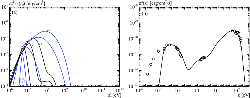
Figure 1.— (a) Evolution of the electron energy distribution with increasing distance $R$ in the steady model. The numbers beside each line denote $R/R_{0}$. The electron spectra during the acceleration phase ($R\leq 2R_{0}$) are plotted with blue lines, while those after the shutdown of the acceleration ($R>2R_{0}$) are black. (b) Photon spectrum for the active period in 2009. The open circles are measured flux points in period D (adapted from Hayashida et al., 2012). The solid line is the model spectrum that is a superposition of the emissions from the all shells of $R>R_{0}$.

As shown in Figure 1 (a), electrons are continuously accelerated between $R=R_{0}$ and $2R_{0}$, then they are rapidly cooled via IC scattering after the shutdown of the acceleration. The electron spectrum at $2R_{0}$ in the low-energy region is consistent with the assumed power-law index of $p=1$ in the broken power-law model of Hayashida et al. (2012). In the highest-energy region, though the Klein–Nishina effect suppresses the IC cooling effect, the synchrotron cooling ($U^{\prime}_{B}=1.9(R/R_{0})^{-2}~{}\mbox{erg}~{}\mbox{cm}^{-3}$) prevent the acceleration above $100$ MeV. The resultant photon spectrum well reproduces the observed spectrum from far-infrared to gamma-ray bands (see Figure 1 (b)). The low-energy cutoff at $\sim 0.02$ eV is due to the synchrotron self-absorption. The X-ray flux is originated from the synchrotron self-Compton (SSC) emission. Those X-ray data strongly constrain the emission radius $R_{0}$.

Thus, our SA model can naturally produce a hard electron spectrum, and the steady photon spectrum agrees with the observed one in 2009. Based on this result, we will probe the intensive flare in 2013 in the next section.

4. Flare Model in 2013

The most intensive flare denoted as period “B” (on MJD 56646) in H15 shows a very hard spectrum with $\Gamma_{\gamma}\sim 1.7$ and a short variability with an hourly scale in the gamma-ray band observed with Fermi-LAT. During a short time interval of the gamma-ray flare period (0.2 days), there were simultaneous optical observations, whose results did not show any correlated variability with the gamma-ray flare as presented in H15. The X-ray observations in the period are available from Swift-BAT transient monitor results by the Swift-BAT team (Krimm et al., 2013). The data provided an upper limit in the 15-50 keV band. We adopt the same values for $R_{0}$, $\Gamma$, $T^{\prime}_{\rm UV}$, and $U^{\prime}_{\rm UV}$ as those in the previous section. By changing $K^{\prime}$, $\dot{N}^{\prime}_{\rm e}$, and $B_{0}$, we attempt to fit the spectrum of the flaring period B in 2013.

We consider one shell that contributes to the flare emission. The energy diffusion coefficient and injection rate are slightly increased from the values in the steady model to $K^{\prime}=1.3\times 10^{-5}~{}\mbox{s}^{-1}$ ($t_{\rm acc}=1/(2K^{\prime})=0.25W^{\prime}/c$), and $\dot{N}^{\prime}_{\rm e}=2.5\times 10^{50}~{}\mbox{s}^{-1}$ ($\dot{n}^{\prime}_{\rm e}=0.85(R/R_{0})^{-2}~{}\mbox{cm}^{-3}~{}\mbox{s}^{-1}$), respectively. Hereafter, we call this the “fiducial” flare model. No significant concurrent flare in the optical bands implies that the optical photons are emitted from other steady components. As discussed in Section 4.3 in H15, the lack of overall correlation between the optical and gamma-ray bands in 2013-2014 also suggests the different origin of the optical component. The synchrotron flux of the flare should be below the observed flux level so that an upper limit for the magnetic field in the flare zone will be given. Here, we adopt a very low value of $B_{0}=0.25$ G.

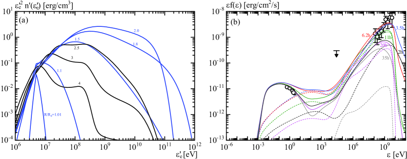
Figure 2.— (a) Evolution of the electron energy distribution with increasing distance $R$ in the fiducial flare model. The figure format is the same as that of Fig. 1(a). (b) Photon spectrum for the most intense flare in 2013. The open circles are measured flux points in period B (adapted from H15), and the $2\sigma$ upper limit for the hard X-ray is obtained from Swift-BAT data. The solid lines are the model spectra at observation times of 2 (black), 3.5 (blue), 6.2 (red), 11 (green), 20 (purple), and 35 (gray) hours. The model parameters for an underlying component, which is consistent with the gamma-ray flux the day before the flare event ($0.19\times 10^{-5}$ photons cm${}^{-2}~{}\mbox{s}^{-1}$ above 0.1 GeV) and the optical data, are the same as those of the steady model in §3 except for $B_{0}=3.8$ G and $\dot{N}^{\prime}_{\rm e}=7.3\times 10^{49}~{}\mbox{s}^{-1}$. The dashed lines show the flare components only. The observation time $t_{\rm obs}$ is measured from the first arrival time of the photons escaped from the shell at $R=R_{0}$. Photons are supposed to be emitted from a single shell moving toward us.

Figure 2 (a) shows the evolution of the electron energy distribution in this flare model. Electrons are accelerated to higher energies compared to the case in the steady model. The power-law distributions above $10^{9}$ eV are due to not only the larger $K^{\prime}$ but also the inefficiency of the synchrotron cooling owing to the low magnetic field. The secondary bumps at $\sim 2\times 10^{8}$ eV for $R=3$-$4R_{0}$ are attributed to the generation of secondary electron–positron pairs via internal $\gamma\gamma$ absorption.

The resultant gamma-ray spectra shown in Figure 2 (b) agree well with the observed gamma-ray data. Here, we add an underlying component (that overlaps the solid gray line in the figure) to explain the gamma-ray flux before the flare and the optical data. The flare spectrum has a higher synchrotron peak energy than the model in H15, since our flare model shows a drastic growth of the maximum energy of electrons compared to the steady model. As remarked above, the weak magnetic field strikingly increases the maximum energy of electrons. Even for this low magnetic field, the optical flux is slightly enhanced during the flare. The steady behavior of the optical light curve may prefer a weaker magnetic field, but we regard this as a conservative upper limit.

The sharp cutoff at $\sim 10^{10}$ eV in the photon spectrum is due to the $\gamma\gamma$ absorption inside the emission region. Some fraction of photons above $10^{10}$ eV escape from the shell. The model flux at the $100$ GeV band is still higher than the detection limit for Čerenkov telescopes. However, it should be noted that we have neglected the $\gamma\gamma$ absorption after the escape from the shell. The absorption by the broad emission lines during propagation may greatly suppress the flux around $100$ GeV.

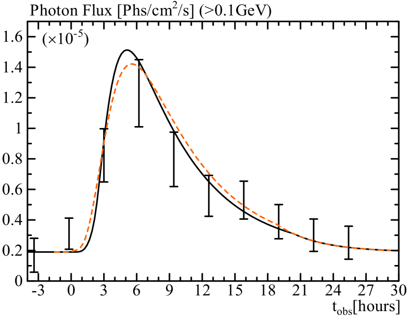
Figure 3.— Gamma-ray light curve of period B in 2013 with the flare model (solid black), and “High-$K$” model (dashed orange). The original data were obtained from H15. In the model light curves, the underlying gamma-ray level is the same as in Fig. 2 ($0.19\times 10^{-5}$ photons cm${}^{-2}~{}\mbox{s}^{-1}$).

Even for the same values of $R_{0}$ and $\Gamma$ as in the steady model, the light curve is well reproduced as shown in Figure 3. Thus, the emission zones of the intense flare in 2013 and the active period in 2009 may be located at similar distances from the central engine. The observed asymmetric profile in the light curve is favorable for our simple one-shell emission-zone model. The strong cooling due to the external IC yields the rapid decay of the light curve. The evolutions of energy densities in Figure 4 clearly show the energy input by the SA and rapid cooling just after the end of the acceleration. At $R=2R_{0}$, the energy density ratio of the magnetic field to electrons is quite low as $U^{\prime}_{B}/U^{\prime}_{\rm e}\sim 4\times 10^{-5}$.

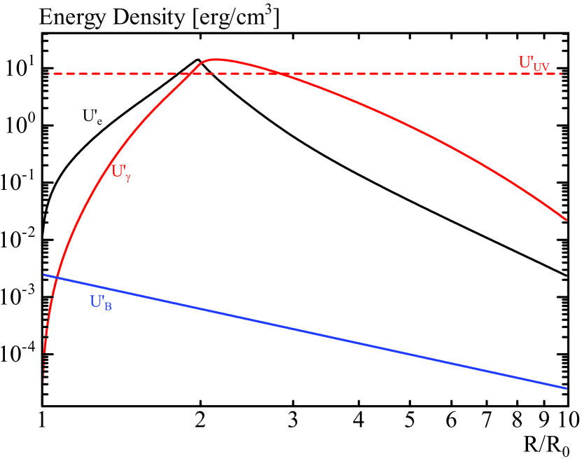
Figure 4.— Evolution of the energy densities in the shell frame for the flare model. The solid black, blue, and red lines show the value of electrons, magnetic fields, and photons produced in the shell, respectively. The red dashed line denotes the value of the external photons.

The observational constraints, of course, do not determine the model parameter uniquely. However, the essential parameter for determining the gamma-ray spectral shape is only $K^{\prime}$ in our model (the role of $\dot{N}^{\prime}_{\rm e}$ is just normalizing the flux level, and the value of $B_{0}$ does not affect the gamma-ray spectral shape). In Figure 5, we compare several photon spectral models derived with different parameter sets. When we reduce $K^{\prime}$ by a factor of two from the fiducial model (“Low-$K$” model: $K^{\prime}\to K^{\prime}\times 0.5$, $\dot{N}^{\prime}_{\rm e}\to\dot{N}^{\prime}_{\rm e}\times 4.8$, the others are the same), the peak photon energy does not reach 10 GeV. Conversely, we increase the diffusion coefficient as shown in the “High-$K$” model ($K^{\prime}\to K^{\prime}\times 1.5$, $\dot{N}^{\prime}_{\rm e}\to\dot{N}^{\prime}_{\rm e}\times 0.038$, $B_{0}\to B_{0}\times 0.4$, the others are the same). In this case, we need an even weaker magnetic field. The peak time of the light curve is delayed due to the lower $\dot{N}^{\prime}_{\rm e}$ compared to the fiducial model. In Figure 3, we shift the light curve by 1.5 hr earlier. Other physical parameters ($\Gamma$, etc.) of the jet were derived from the steady model. However, as H15 supposed, we also try to increase $\Gamma$ in our model. The initial radius should be increased as $\propto\Gamma^{2}$ to keep the variability timescale. Such an example (“High-$\Gamma$” model: $\Gamma\to\Gamma\times 2$, $R_{0}\to R_{0}\times 4$, $\dot{N}^{\prime}_{\rm e}\to\dot{N}^{\prime}_{\rm e}\times 0.039$, $B_{0}\to B_{0}\times 0.16$, $K^{\prime}$ is the same) is shown in Figure 5. Due to the relatively short $t_{\rm acc}$ ($=0.18W^{\prime}/c$), the maximum electron energy grows as high as $\varepsilon^{\prime}_{\rm e}\sim 10^{13}$ eV. A very low magnetic field ($U^{\prime}_{B}/U^{\prime}_{\rm e}\lesssim 6\times 10^{-5}$) is necessary again to suppress the synchrotron flux in the X-ray band. The strong cooling due to the higher $U^{\prime}_{\rm UV}\propto\Gamma^{2}$ makes the GeV spectrum too soft compared to the observed gamma-ray spectrum.

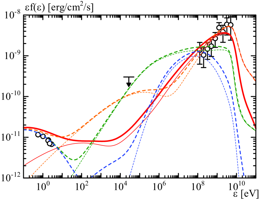
Figure 5.— Comparison of the model spectra at $t_{\rm obs}=6.2$ hr: the same model as in Fig. 2 (solid red), “High-$K$” model (dashed orange), “Low-$K$” model (dashed blue), and “High-$\Gamma$” model (dashed green). The steady underlying component is included as in Figure 2. The thin lines show the flare component only.

5. Discussion

The simple SA model can reasonably explain the very hard spectrum and short variability in the intensive flare in 2013. The turbulence driving the particle acceleration may be generated by the hydrodynamical instability or the magnetic reconnection.

Compared to the steady model for the active period in 2009, the drastic alteration we need is the decrease of the magnetic field. The other parameters have almost similar values. The absence of the optical flare implies the weak magnetic field ($<0.25$ G). The requirement of the magnetic field decrease at gamma-ray flare stages was suggested by Asano et al. (2014) as well. The required low magnetic field seems irrelevant to the energy source for the particle acceleration. Therefore, a hydrodynamical instability is responsible for driving the SA.

When $\Gamma=15$, the variability timescale is consistent with $R_{0}=0.02$ pc as shown in Figure 3. This distance from the engine also agrees with the constraint by the X-ray SSC component in the active period in 2009. The size of the central engine may be $\sim 3r_{\rm g}\sim 8.6\times 10^{-5}$ pc for the black hole mass of $3\times 10^{8}M_{\sun}$. If we adopt the simplest model for the jet acceleration due to the magnetic energy dissipation (Drenkhahn, 2002), the bulk Lorentz factor at $R=R_{0}$ should be $<(R_{0}/3r_{\rm g})^{1/3}\sim 6$, which is inconsistent with the postulated value of $\Gamma$. Given the variability timescale $\Delta t$, the initial radius can be scaled as $R_{0}\propto\Delta t\Gamma^{2}$ when we change $\Gamma$. However, even in this case, the maximum Lorentz factor at $R_{0}$ inferred from the magnetic dissipation model increases by a factor of only $R_{0}^{1/3}\propto\Gamma^{2/3}$. For the jet acceleration model by the Poynting flux dissipation, not only the low magnetic field but also the short variability timescale are problematic. This problem is also raised for the very short gamma-ray flare (a few hundreds seconds) of BL Lac objects like PKS 2155–304 (Aharonian et al., 2007). For such SSC-dominant objects, however, the distance from the engine is not well constrained compared to FSRQs.

The tiny change of the diffusion coefficient $K^{\prime}$, in spite of the drastic decrease of the magnetic field, seems enigmatic. The assumed value of $q=2$ may be favorable for this invariant behavior of $K^{\prime}$. In this low magnetic field case, the average energy gain per scattering may be proportional to $\beta_{\rm W}^{2}$, where $\beta_{\rm W}$ is the average turbulence velocity, rather than the Alfvén velocity. The pitch angle diffusion approximation (Blandford & Eichler, 1987) and power-law magnetic turbulence of $\delta B^{2}(k)=\delta B_{0}^{2}k^{-q}$, where $k$ is the wavenumber, leads to $K\propto\beta_{\rm W}^{2}\delta B_{0}^{2}B^{-q}$. The last factor of $B^{-q}$ implies that electrons interact with higher (lower) amplitude turbulence at longer (shorter) wavelengths for a weaker (stronger) magnetic field. If $\delta B_{0}\propto B$, $q=2$ results in $K\propto\beta_{\rm W}^{2}$, which is independent of $B$. Alternatively, magnetic bottles as “hard spheres” (Beresnyak, Yan & Lazarian, 2011) may be formed in turbulence independently of the strength of the magnetic field. Such requirements for the turbulence property motivate us to probe the hydrodynamical instabilities in blazar jets.

References

- Abdo et al. (2010a) Abdo, A. A., Ackermann, M., Ajello, M., et al. 2010, ApJ, 710, 810
- Abdo et al. (2010b) Abdo, A. A., Ackermann, M., Ajello, M., et al. 2010, Nature, 463,919
- Ackermann et al. (2015) Ackermann, M., Ajello, M., Atwood, W., et al. 2015, arXiv:1501.06054
- Aharonian et al. (2007) Aharonian, F., Akhperjanian, A. G., Bazer-Bachi, A. R., et al. 2007, ApJ, 664, L71
- Asano et al. (2014) Asano, K., Takahara, F., Kusunose, M., Toma, K., & Kakuwa, J. 2014, ApJ, 780, 64
- Beresnyak, Yan & Lazarian (2011) Beresnyak, A., Yan, H., & Lazarian, A. 2011, ApJ, 728, 60
- Blandford & Eichler (1987) Blandford, R., & Eichler, D. 1987, PhR, 154, 1
- Błażejowski et al. (2005) Błażejowski, M., Blaylock, G., Bond, I. H., et al. 2005, ApJ, 630, 130
- Brandenburg, Kahniashvili & Tevzadze (2015) Brandenburg, A., Kahniashvili, T., & Tevzadze, A. G. 2015, Phys. Rev. Lett., 114, 075001
- Chen et al. (2011) Chen, X., Fossati, G., Liang, E. P., & Böttcher, M. 2011, MNRAS, 416, 2368
- Diltz & Böttcher (2014) Diltz, C., & Böttcher, M. 2014, J. High Ene. Astrop., 1, 63
- Drenkhahn (2002) Drenkhahn, G. 2002, A&A, 387, 714
- Fossati et al. (2008) Fossati, G., Buckley, J. H., Bond, I. H., et al. 2008, ApJ, 677, 906
- Hayashida et al. (2012) Hayashida, M., Madejski, G. M., Nalewajko, K., et al. 2012, ApJ, 754, 114
- Hayashida et al. (2015) Hayashida, M., Nalewajko, K., Madejski, G. M., et al. 2015, ApJ, 807, 79
- Janiak et al. (2012) Janiak, M., Sikora, M., Nalewajko, K., et al. 2012, ApJ, 760, 129
- Kakuwa et al. (2015) Kakuwa, J., Toma, K., Asano, K., Kusunose, M., & Takahara, F. 2015, MNRAS, 449, 551
- Katarzyński et al. (2006) Katarzyński, K., Ghisellini, G., Mastichiadis, A., Tavecchio, F., & Maraschi, L. 2006, A&A, 453, 47
- Krawczynski, Coppi & Aharonian (2002) Krawczynski, H., Coppi, P. S., & Aharonian, F. 2002, MNRAS, 336, 721
- Krawczynski et al. (2004) Krawczynski, H., Hughes, S. B., Horan, D., et al. 2004, ApJ, 601, 151
- Krimm et al. (2013) Krimm, H. A., Holland, S. T., Corbet, R. H. D., et al. 2013, ApJS, 209, 14
- Kusunose, Takahara & Li (2000) Kusunose, M., Takahara, F., & Li, H. 2000, ApJ, 536, 299
- Lazarian et al. (2012) Lazarian, A., Vlahos, L., Kowal, G., Yan, H., Beresnyak, A., de Gouveia Dal Pino, E. M. 2012, Space Sci. Rev., 173, 557
- Lefa, Rieger & Aharonian (2011) Lefa, E., Rieger, F. M., & Aharonian, F. 2011, ApJ, 740, 64
- Matsumoto & Masada (2013) Matsumoto, J., & Masada, Y. 2013, ApJ, 772, L1
- Mizuno, Hardee & Nishikawa (2007) Mizuno, Y., Hardee, P. E., & Nishikawa, K. 2007, ApJ, 662, 835
- Pacciani et al. (2014) Pacciani, L., Tavecchio, F., Donnarumma, I., et al. 2014, ApJ, 790, 45
- Stawarz & Petrosian (2008) Stawarz, Ł., & Petrosian, V. 2008, ApJ, 681, 1725
- Wehrle et al. (1998) Wehrle, A. E., et al. 1998, ApJ, 497, 178
- Zrake (2014) Zrake, J. 2014, ApJ, 794, 26