∥
ANNz2 - photometric redshift and probability
distribution function estimation using machine learning
Abstract
We present ANNz2, a new implementation of the public software for photometric redshift (photo-) estimation of Collister and Lahav (2004), which now includes generation of full probability distribution functions (PDFs). ANNz2 utilizes multiple machine learning methods, such as artificial neural networks and boosted decision/regression trees. The objective of the algorithm is to optimize the performance of the photo- estimation, to properly derive the associated uncertainties, and to produce both single-value solutions and PDFs. In addition, estimators are made available, which mitigate possible problems of non-representative or incomplete spectroscopic training samples. ANNz2 has already been used as part of the first weak lensing analysis of the Dark Energy Survey, and is included in the experiment’s first public data release. Here we illustrate the functionality of the code using data from the tenth data release of the Sloan Digital Sky Survey and the Baryon Oscillation Spectroscopic Survey. The code is available for download at https://github.com/IftachSadeh/ANNZ .
1 Introduction
1.1 Photometric redshifts
Redshifts, usually denoted by , effectively provide a third, radial dimension to Cosmological analyses. They allow the study of phenomena as a function of distance and time, as well as enable the identification of large structures, such as galaxy clusters. The current and next generations of dark energy experiments, such as the Dark Energy Survey (DES),111 See http://www.darkenergysurvey.org . the Large Synoptic Survey Telescope (LSST),222 See http://www.lsst.org . and the Euclid experiment333 See http://sci.esa.int/euclid/ . will collectively observe a few billion galaxies. Ideally, redshifts may be measured with great precision using spectroscopy. However, it is infeasible to obtain spectra for such large galaxy samples. The success of these imaging surveys is therefore critically dependent on the measurement of high-quality photometric redshifts (photo-s). For instance, a benchmark of LSST is to measure the dark energy equation of state parameter, , with per-cent level uncertainty. This is expected to be achievable with weak lensing tomography (Hu, 1999; Zhan and Knox, 2006). However, it will require a precision of in determination of the systematic bias in the redshift.
This paper presents ANNz2. The latter is a new implementation of the code of Collister and Lahav (2004), denoted hereafter as ANNz1, which used artificial neural networks to estimate photometric redshifts. ANNz2 is free and publicly available.444 See https://github.com/IftachSadeh/ANNZ . The code has already been incorporated as part of the analysis chain of DES (Sánchez et al., 2014). It has been shown to provide reliable photo- estimates and to reduce systematic uncertainties and outlier contamination (Leistedt et al., 2015). ANNz2 photo-s were part of the first DES weak lensing analysis (DES Collaboration, 2015; Bonnett et al., 2015), are included in the first public data release of the project,555 See http://des.ncsa.illinois.edu/releases/sva1 . and are being used for upcoming analyses.
The extensive work in the community on photo-s usually falls into two categories, papers on particular methods (see below) and studies comparing existing methods (Abdalla et al., 2011; Sánchez et al., 2014). The new ingredient of the present paper is a new approach to contrast and combine different machine learning techniques, and to yield self-consistently a photo- probability distribution function (PDF). The introduction of PDFs has been shown to improve the accuracy of Cosmological measurements (Mandelbaum et al., 2008; Myers et al., 2009), and is an important new feature compared to the previous version of the code. In addition to photo- inference, it is also possible to run ANNz2 in classification mode. The latter is useful for analyses such as star/galaxy separation and morphological classification of galaxies. An example is provided as part of the software package, but is not discussed in the following.
In the next section we present a short overview of the current methodology for deriving photometric redshifts, focusing on machine learning, and on the techniques available through ANNz2. We then describe the main methods implemented in the code for estimating photo-s and PDFs, and illustrate the performance using a toy analysis. A short quick-start guide for using the code is presented in the appendix.
1.2 Methodology for photo- estimation
The different approaches to calculate photo-s can generally be divided into two categories, template fitting methods and training based machine learning. Both types depend heavily on photometric information, such as the integrated flux of photons in medium- or broad-band filters, which are usually converted into magnitudes or colours. The magnitudes serve as a rough measurement of the underlying spectral energy distribution (SED) of a target object, from which the redshift may be inferred. A review of current photo- methods can be found in Abdalla et al. (2011); Hildebrandt et al. (2010). All methods require a spectroscopic dataset for training and/or calibration, the requirements for which are discussed by Newman et al. (2015).
Template fitting methods involve fitting empirical or synthetic galaxy spectra with the photometric observables of an imaging survey, accounting for the response of the telescope and the properties of the filters (Benítez et al., 2009; Mobasher et al., 2007). The template spectra are generally derived from a small set of SEDs, representing different classes of galaxies at zero redshift. They also incorporate astrophysical effects, such as dust extinction in the Milky Way or in the observed galaxy. Common template libraries are the Coleman et al. (1980) SEDs (derived observationally), or those of Bruzual A. and Charlot (1993) (based on synthetic models).
Template methods rely on the assumption that the SED templates are a true representation of the observed SEDs. They depend e.g., on proper calibration of the rest-frame spectra of galaxies, commonly performed using spectroscopic data. In addition, the composition of the template library should correspond to the population of galaxies which are fitted (for instance, in terms of galaxy types and luminosities). Photo-s may be estimated by choosing the best-fitted SED from the template library, usually derived using - minimization (Bolzonella et al., 2000), where more advanced Bayesian priors can also be incorporated (Benitez, 2000).
On the other hand, empirical methods do not directly use physically motivated models. Instead, they involve deriving the relationship between the photometric observables and the redshift using a so-called training dataset, which includes both the observables and precise redshift information. The mapping between observables and the output redshift can be as simple as a polynomial fit (Connolly et al., 1995). However, supervised machine learning methods (defined below)666 Un-supervised learning techniques have been used to derive photometric redshifts as well (see e.g., Geach (2012); Way and Klose (2012); Carrasco Kind and Brunner (2014)), but are not discussed here. have been shown to produce much more accurate and robust results, taking into account complicated correlations between the input parameters and the output value.
Machine learning methods have several advantages over template fitters. For instance, it is trivial to incorporate additional observables into the inference, a common example being the surface brightness of galaxies, which has a redshift dependence (Firth et al., 2003). In addition, the use of a training sample alleviates systematic side-effects associated with the photometry, such as errors in the zero-point corrections of the magnitudes. On the other hand, the size and composition of the training sample become important factors in the performance. The phase space of input parameters and the spectral types of galaxies must correspond to the respective parameters of the survey. If this is not the case, the photo-s of certain galaxy populations may become biased (Hoyle et al., 2015a). Another important point, is that the true redshift distribution in the spectroscopic training set must also be representative of the survey. In particular, machine learning methods are only reliable within the redshift range of the galaxies used for the training. Consequently, they should not be used to infer the photo-s of very high-redshift sources, for which there are no spectroscopic training data. In order to resolve these problems, it is possible to generate synthetic training galaxies within the required parameter space, using template-SED libraries. However, this introduces some of the systematic biases associated with template fitting methods.
An important element of any photo- algorithm is calculation of the associated uncertainty. Accurate photo- uncertainties help to identify catastrophic outliers, the removal of which may improve the quality of Cosmological analyses (Abdalla et al., 2008; Banerji et al., 2008). For the previous version of the code, ANNz1, uncertainties were derived using a chain rule, propagating the uncertainties on the algorithm-inputs (e.g., magnitudes) to an uncertainty on the final value of the photo-. Other methods exist (Oyaizu et al., 2008), which use the training data and the photo-s themselves for uncertainty estimation. In these cases, the uncertainty is parametrized as a function of the inputs to the algorithm, requiring no measurement of the uncertainties on the individual inputs. We use such a scheme in ANNz2 (see Sect. 4.2).
The common method for deriving the uncertainties for template fitting methods is by combining the likelihoods estimated for the various templates. The benefit of performing the combination is that it naturally leads to the definition of a photo- PDF, as, for instance, is the case in Le PHARE (Arnouts et al., 1999; Ilbert et al., 2006), BPZ (Benitez, 2000) and ZEBRA (Feldmann et al., 2006). As for machine learning methods, there is a variety of codes on the market. These use different methods besides artificial neural networks, such as boosted decision trees. While most algorithms produce only single-value photo-s, several also generate photo- PDFs, such as ArborZ (Gerdes et al., 2010), TPZ (Carrasco Kind and Brunner, 2013), SkyNet (Bonnett, 2015) and the algorithm of Rau et al. (2015). In ANNz2, two primary types of PDF are derived, one of which represents a new technique, while the other is similar in nature to the PDFs generated by ArborZ, TPZ and SkyNet.
In the following, we describe in more detail the general workings of machine learning, focusing on the primary algorithms used in ANNz2.
1.3 Machine learning methods
1.3.1 Basics of machine learning
Machine learning methods (MLMs) use supervised learning, a machine learning task of inferring a function from a set of training examples. Each example consists of an input object, described by a collection of input parameters, as well as a desired output value for the MLM. The training examples are used to determine the mapping for either classification or regression problems. The former describes a decision boundary between signal and background entries; the latter refers to an approximation of the underlying functional behaviour defining the output.
For the purpose of creating an MLM estimator for either classification or regression, one generally splits the available dataset of examples into three parts, designated as the training, validation and testing samples. The training dataset is used for deriving the desired mapping between the input and the output. During each step of the training, the validation sample is used to estimate the convergence of the solution, by comparing the result of the estimator with the value of the output. The testing dataset is not used during the training process; rather, it is utilized as an independent test of the performance of the trained MLM.
The MLMs utilized in ANNz2 are implemented in the TMVA package777 See http://tmva.sourceforge.net . (Hoecker et al., 2007), which is part of the ROOT C software framework888 See http://root.cern.ch . (Brun and Rademakers, 1997). TMVA includes multiple MLM methods, all of which are available through ANNz2, using a common Python interface with simple control-options (see Appendix A). The two TMVA MLMs which we found to be most appropriate for the problem of photo- estimation, are artificial neural networks and boosted decision/regression trees. For completeness, these are outlined concisely in the following. Detailed descriptions of the implementation may be found in the TMVA manual. For a comprehensive theoretical overview, see MacKay (2003); Hastie et al. (2001).
1.3.2 Available methods in TMVA
- Artificial neural networks (ANNs). One may consider an ANN as a mapping between a set of input variables, such as magnitudes or colours, and one or more output variables. For regression problems, the output is e.g., the numerical value of a photometric redshift. For classification, the output is a variable (usually between and ), which may be used to discriminate between signal and background examples. The mapping is performed by computing the weighted sum of a collection of response functions. The input variables, response functions and output variables are collectively called neurons. The response may be represented by various activation functions, such as sigmoid or tanh functions.
In ANNz2, the TMVA method for ANNs called a multi-layer perceptron is implemented. In this case, ANN neurons are organized into at least three layers, the input layer; a hidden layer; and the output layer, where more complicated structures may include multiple hidden layers. A schematic illustration is shown in Fig. 1.
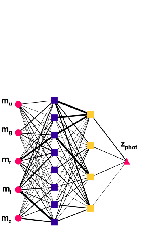
In the perceptron, the response of a neuron is fed into the next layer (up to the output), using a series of relative weights. Learning occurs by changing the inter-neuron weights after each element of the dataset is processed, using the so-called back propagation algorithm. This is carried out through a generalization of the least mean squares algorithm, using the ANN error function. The latter characterizes the amount of error in the output compared to the predicted result in the validation dataset. In practice, the weights are varied using the gradient of the error function, though optionally, the second derivatives of the error may also be used.
Using ANNs, it is important to avoid over-training. The latter occurs when an ANN becomes sensitive to the fluctuations in a dataset, instead of to the coherent features of the observables which should be mapped to the output. Over-training leads to a seeming increase in the performance, if measured on the training sample. Conversely, it also results in an effective performance decrease, when measured from the independent validation sample. Over-training may therefore be detected by comparing the value of the error estimator between the training and the validation sample. In addition to testing for over-training, convergence tests may also be performed. The latter refer to checking whether the estimator has ceased to improve over the course of several training cycles; they are used in order to determine when to stop training
An additional feature available in TMVA is Bayesian regularization. Regularization adds a term to the error function of the ANN, which is equivalent to the negative value of the log-likelihood of the training data, given the network model. Regularization reduces the risk of over-training, by penalizing ANNs with over-complicated architectures (too many degrees of freedom).
- Boosted decision trees (BDTs). A decision or regression tree999 We use here the terms decision- and regression-trees interchangeably. is a binary tree, in which decisions are taken on one single variable at a time, until a stop criterion is fulfilled. The decision tree splits the parameter space into a large number of hypercubes. Each of these is attributed a constant target value for regression, or identified as either “signal-like” or “background-like” for classification. The various output nodes are referred to as leafs. The path down the tree to each leaf represents an individual cut sequence that narrows down the value of the regression target, or the identification as signal or as background. A schematic representation of a decision tree is shown in Fig. 2.
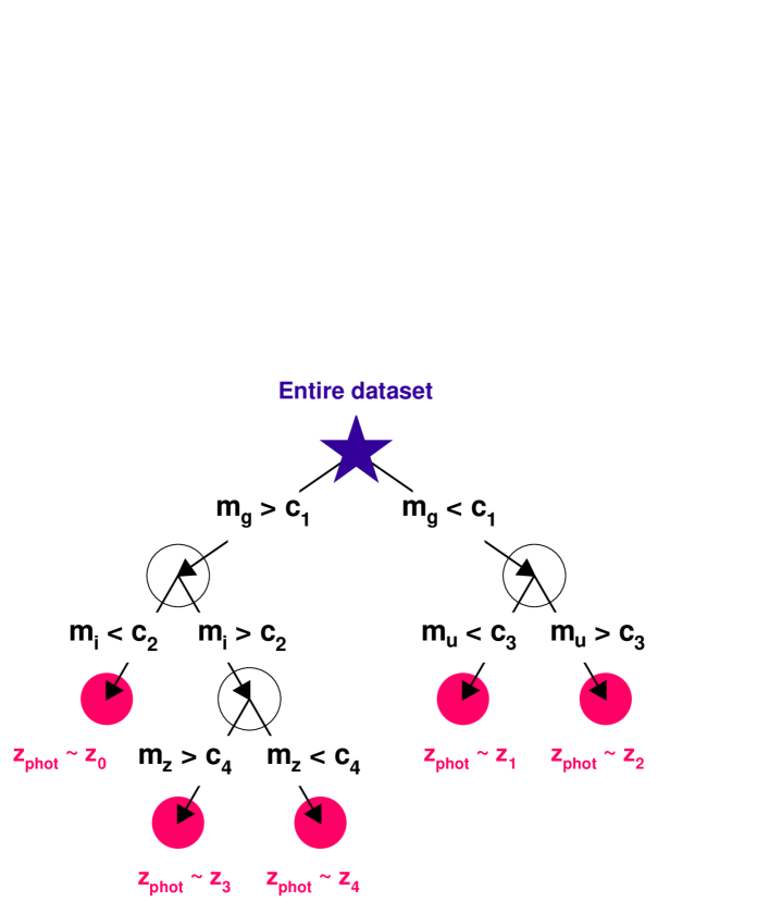
The training, or growing, of a decision tree is the process that defines the splitting criteria for each node, the purpose of which is to achieve the best estimation of the regression target, or the best separation between signal and background objects. The training starts with the root node, which is split into two subsets of training objects. In each subsequent step, further splitting occurs. At each node, the split is determined by finding the variable and corresponding cut value that provide the best discriminatory power. Training stops when the minimum number of training examples in a single leaf is reached, according to a predefined threshold value. For regression, each leaf corresponds to the value of the regression target of the associated training examples. For classification, a leaf is interpreted as signal or as background, based on the type of the majority of corresponding examples. Different splitting criteria can be selected by the user in ANNz2, among other algorithm parameters.
Decision trees are sensitive to statistical fluctuations in the training sample. This comes about, as a small change in a single node may affect all subsequent nodes, and the entire structure of the tree thereafter. It is therefore beneficial to use not a single tree classifier, but a forest of trees, by using a boosting algorithm. The process of boosting involves training multiple classifiers using the same data sample, where the data are reweighted differently for each tree. The combined estimator is then derived from the weighted majority vote of trees in the forest. Alternatively, it is also possible to use bagging instead of boosting. In the bagging approach, a re-sampling technique is used; a classifier is repeatedly trained using re-sampled training objects such that the combined classifier represents an average of the individual classifiers. Several boosting/bagging algorithms are implemented in TMVA, all available through ANNz2.
- Other methods. The TMVA package includes several other machine learning methods which are not discussed here, such as k-nearest neighbours, support vector machines, multidimensional likelihood estimators and function discriminant analysis. All of these are interchangeable in ANNz2; the user may choose any type or combination of types of MLM, in order to derive single-value solutions and PDFs.
1.3.3 Method selection and parameter tuning
Different MLMs have their own strengths and weaknesses. For instance, the training of a BTD is generally much faster than e.g., that of an ANN; conversely, the evaluation time of ANNs is generally shorter than that for large random forests. In order to select the best estimator for a given problem, it is recommended to derive solutions using multiple methods, using various choices of algorithm parameters. This is done in an automated fashion in ANNz2.
2 Example analysis
The ANNz2 package is provided with a small dataset, used as a toy analysis. The data consist of observations of galaxies and stars, included in the tenth data release (DR10) of the Sloan Digital Sky Survey (SDSS) (Ahn et al., 2014), including measurements taken with the Baryon Oscillation Spectroscopic Survey (BOSS) (Dawson et al., 2013).
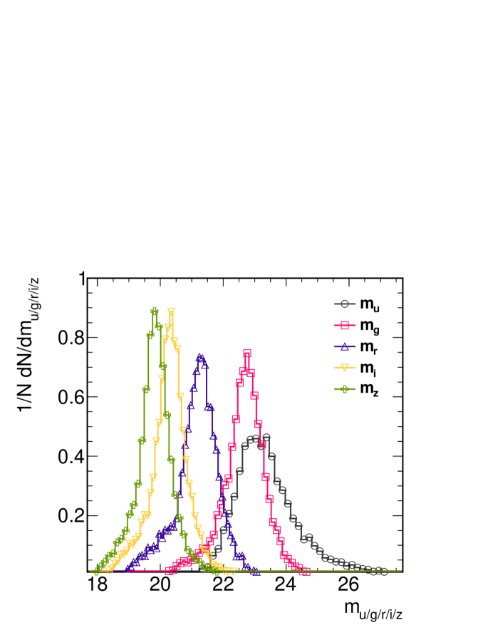
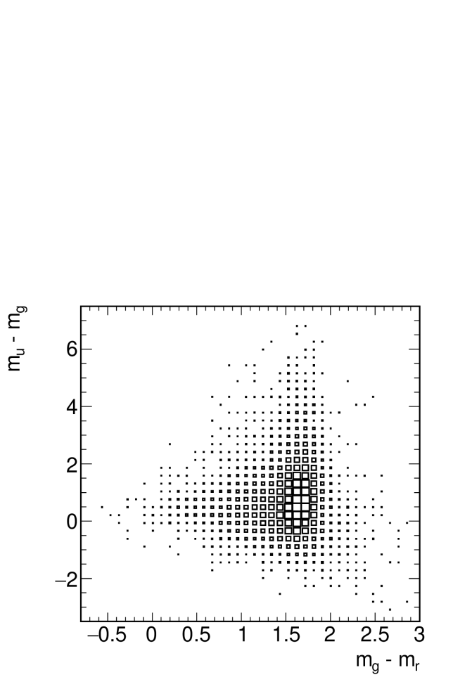
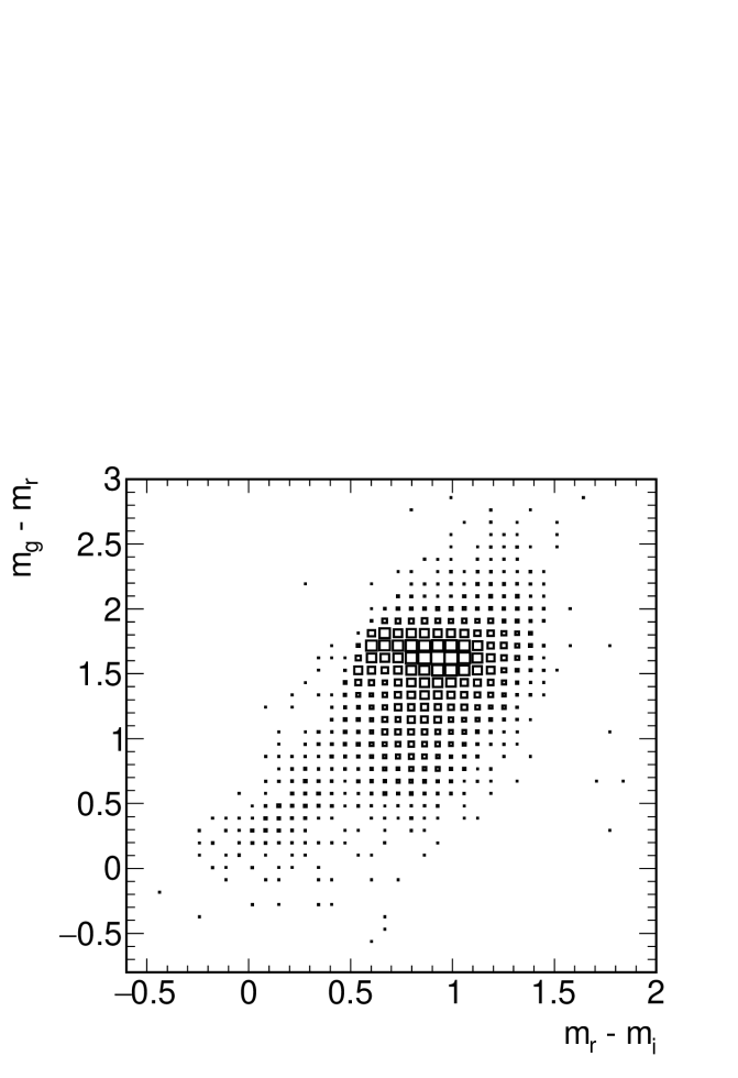
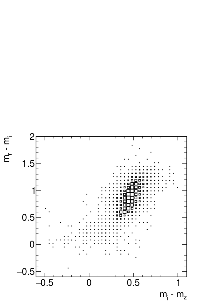
The galaxy sample used for the photo- analysis is derived from a publicly available catalogue.101010 See http://www.sdss3.org/dr10/spectro . The inputs for the photo- inference are Pogson galaxy magnitudes in five bands (ugriz). The magnitudes, m, were calculated from the provided flux measurements, f, using the relation, The general properties of the dataset, comprised of roughly objects, are shown in Fig. 3.

3 Definition of metrics and notation
In order to quantify the performance of the different configurations of ANNz2, several metrics are used. The metrics serve both as part of the dynamic optimization procedure of ANNz2, and as a means of assessing the quality of the results. All calculations take into account per-object weights. Weights may be defined by the user, or derived on the fly based on the type of analysis. For instance, the user may choose to down-weight certain galaxies based on an associated degree of confidence. Such a sub-sample would then have lower relative significance during training and optimization. Weights are also used in order to account for unrepresentative training samples, as described in Sect. 4.4.
The following metrics are used. The photometric bias of a single galaxy is defined as , where and are respectively the photometric and spectroscopic redshifts of the galaxy. The photometric scatter represents the standard deviation of for a collection of galaxies. Similarly, denotes the half-width of the area enclosing the peak of the distribution of . Another useful qualifier is the outlier fraction of the bias distribution, , defined as the percentage of objects which have a bias larger than some factor, , of either or . In addition, we also define the combined outlier fraction for 2 and , .
The various metrics are calculated for galaxies in bins of either or , and are denoted in the following by a subscript, , as , , and . The average values of the metrics over all redshift bins are denoted by , , and , and serve as single-value qualifiers of the entire sample of galaxies.
The purpose of the bias, scatter and outlier fractions is to qualify the galaxy-by-galaxy photo- estimation. Additionally, the overall fit of the photometric redshift distribution, , to the true redshift distribution, , is assessed using two metrics. The first is denoted by , and stands for the sum of the bin-wise difference between the two distributions, normalized by the Poissonian fluctuations. The second measure is the value of the Kolmogorov-Smirnov (KS) test of and , which stands for the maximal distance between the cumulative distribution functions of the two distributions. The -test has the advantage that, unlike , it does not depend on the choice of binning of the redshift distributions. The absolute value of the and -test statistics is not necessarily significant. Rather, these serve to compare the compatibility of the and distributions, between different photo- estimators.
4 The ANNz2 algorithm
4.1 Photo- PDF derivation
The primary configurations of ANNz2 are referred to as single regression and randomized regression. These are respectively used to derive single-value solutions and PDFs. The PDFs provided by ANNz2 are intended to provide a description of our knowledge of the photo- solution. Assuming one could reconstruct a perfect photometric redshift, the corresponding PDF would be given by a delta function. However, the redshift inference has intrinsic uncertainties. A photo- PDF can thus be thought of as a way to parametrize the uncertainty on the solution.
The main contributing factors to the uncertainty on photo-s are the following:
-
1.
Uncertainty on inputs to training: magnitudes are not sufficient to derive the redshift, as they only provide a rough sampling of the underlying SED. Furthermore, one also needs to consider the uncertainties on the values of the magnitudes. The latter are usually derived from the Poissonian noise on the corresponding photon-count, and so are under-estimated. These uncertainties are therefore difficult to take into account in the photo- derivation in a direct way.
-
2.
Uncertainty on MLMs: there is an inherent uncertainty on the solution of a given MLM. For example, different initial random seeds for training, or the choice of different MLM algorithms, may result in variation in the performance.
-
3.
Unrepresentative training datasets: the training data may not be representative of the evaluated photometric sample. In this case, the results are influenced by the composition of the training dataset (the relative proportion of training galaxies with different combinations of magnitudes).
-
4.
Incomplete training datasets: the training data may not be complete. This may occur if some regions of magnitude-space, which exist in the evaluated sample, have no corresponding galaxies for training. The photo- predictions for such evaluated galaxies are unreliable.
Of these sources of uncertainty, the first three may be incorporated into a meaningful PDF. The dominant effect of the latter is the degenerate mapping between magnitudes and redshift . As an example, one may consider the small gap between the response curves of the SDSS g- and r-band filters. The latter results in an ambiguity in the location of the Balmer break between the two bands, for galaxies with (Schmidt, 2007). The degeneracy manifests itself as large photo- uncertainties for this redshift region, as e.g., evident from Fig. 4(a) below.
Glossing for the moment over the the technical details, the procedure for deriving our PDF is as follows. We start by producing a single-value photo- solution. We then combine this solution with the corresponding photo- uncertainty due to the training inputs , which is derived as explained in Sect. 4.2. The procedure is repeated for an ensemble of MLM estimators. The MLMs differ from each other in the choice of algorithm and of algorithm settings, e.g., numbers of neurons in an ANN, number of trees in a BDT and so forth . The various estimators and their corresponding uncertainties are then combined into a PDF, as detailed in Sect. 4.3.
In general, the variance between different estimators is sub-dominant compared to the photo- uncertainty on a single MLM. However, the combination of different estimators allows for the reconstruction of multi-peak PDFs, exposing degeneracies. This comes about, as each MLM is sensitive to different statistical fluctuations. Subsequently, each MLM has a slightly different response in cases where the photo-/redshift relation is ambiguous. Using multiple MLMs also has the advantage of exposing configurations which perform badly due to a poor choice of algorithm parameters, or to a statistical fluctuation in the training. Conversely, consider an example where e.g., a pair of ANNs with different numbers of neurons exhibit slightly different performance. Combining several solutions takes away some of the arbitrariness of selecting one specific model.
The uncertainties on the make-up of the training dataset can only partially be addressed. To deal with unrepresentative training samples, we employ training weights. The latter are used to match the distribution of the inputs (e.g., magnitudes) from the training sample, to those from the evaluated data (Lima et al., 2008). The calculation of the weights is performed as part of the internal pipeline of the code. The issue of incomplete training samples can not be taken into account without the use of additional data (such as those derived from simulations or from template libraries). ANNz2 therefore provides a quality flag, which indicates when unrepresented data are being evaluated. A short discussion is given in Sect. 4.4.
An alternative type of PDF is also generated by ANNz2, using the binned classification configuration. This approach has been used in the past, following the methodology of Gerdes et al. (2010). In binned classification, we build up a PDF by estimating the local photo- probability in narrow redshift regions, implementing classification MLMs instead of regression. We have found that this method tends to under-perform compared to randomized regression. Binned classification is therefore not discussed here further, though an example analysis is provided with the software package.
In the next sections, we describe in detail the ANNz2 algorithm. All figures in the following are based on testing data (galaxies which were not used as part of the training/validation phase).
4.2 Single regression and uncertainty estimation
In the simplest configuration of ANNz2, a single regression is performed. This is similar to the nominal product of the original version of the code, ANNz1.
We compare the output of ANNz2 with that of ANNz1 in Fig. 4.
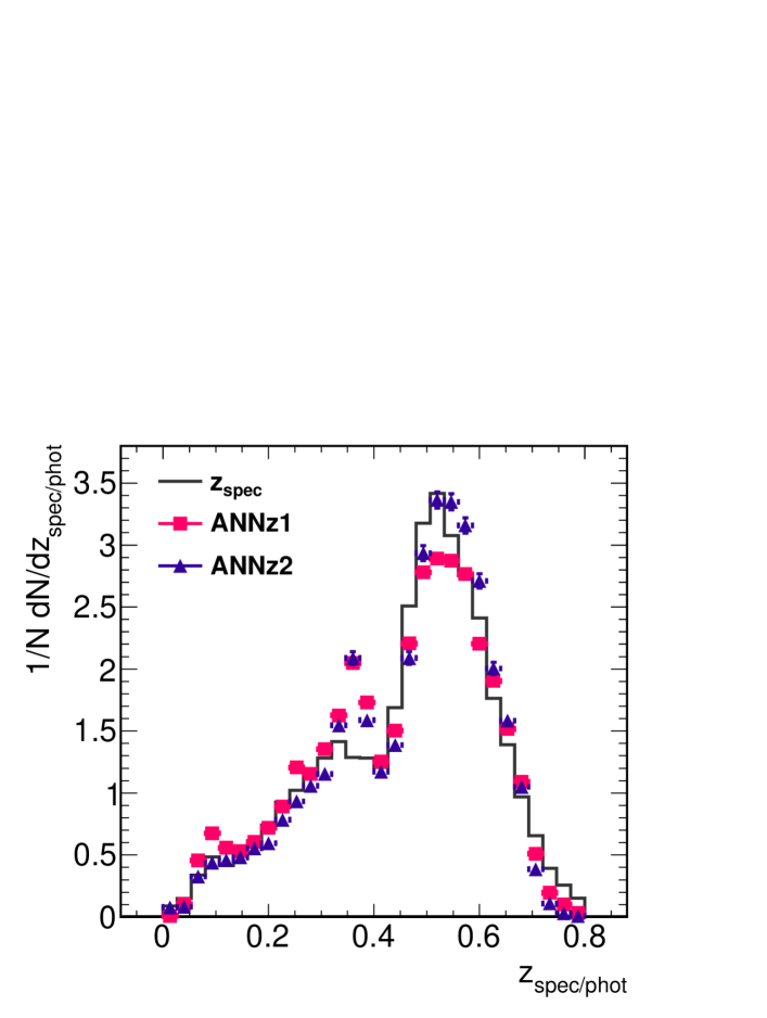
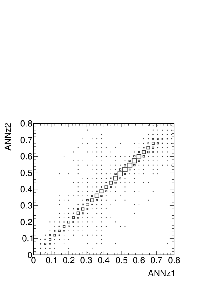
In both cases, a single ANN with architecture was used; this corresponds to input parameters (five magnitudes) in the first layer, three hidden layers with various numbers of neurons, and one output neuron in the final layer.111111 This network architecture was found to produce optimal performance for our particular dataset, and is denoted below as . However, for a different analysis, another architecture might be preferred. A sample of objects was used for the training. Comparable results were also achieved, using as many as , and as few as objects.
The redshift distributions derived by the two versions of the code are similar, with somewhat better performance of ANNz2 over the original version. One may notice the large uncertainty on the photo-s around for both estimators, as mentioned above. Such discrepancies between the derived photo-s and the true redshift are difficult to reconcile using a single-value MLM. However, a PDF solution helps to alleviate the problem (see Figure 9 below). In order to understand how to derive a PDF, we must first qualify the performance of a single MLM.
The relation between the spectroscopic redshift and the photo- estimator of ANNz2 is shown in Fig. 5(a).
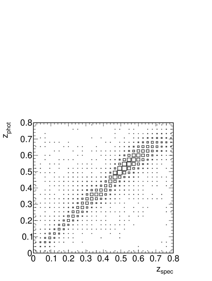
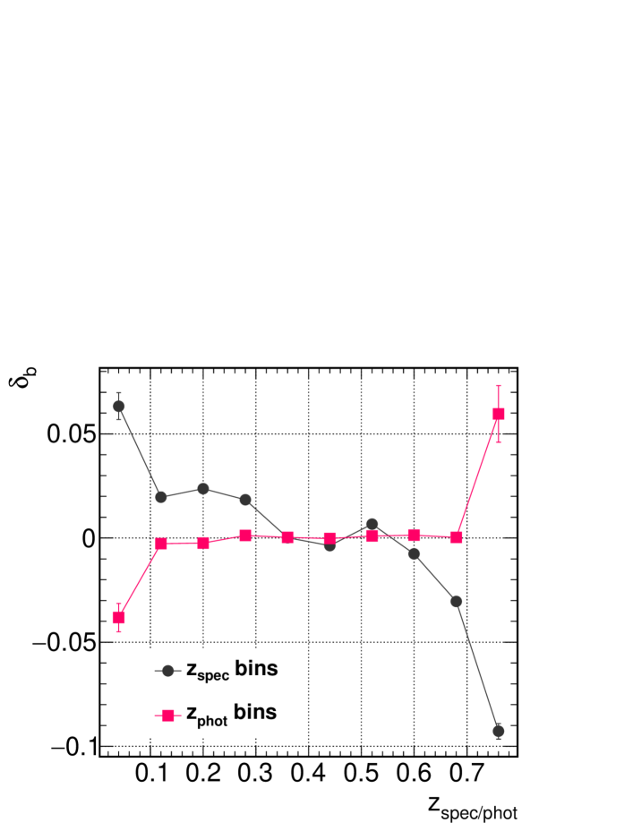
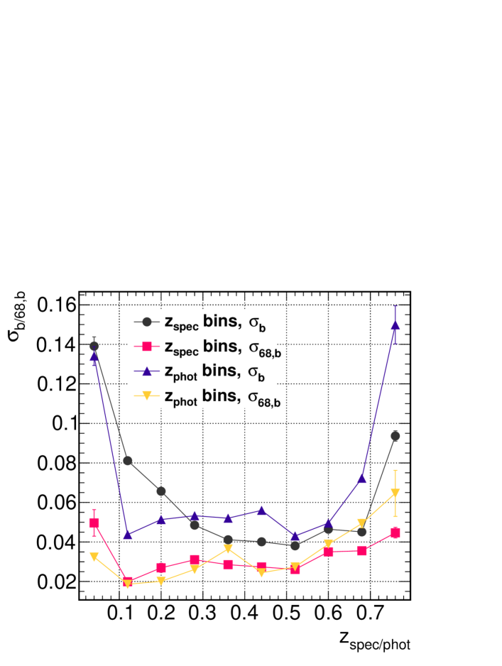
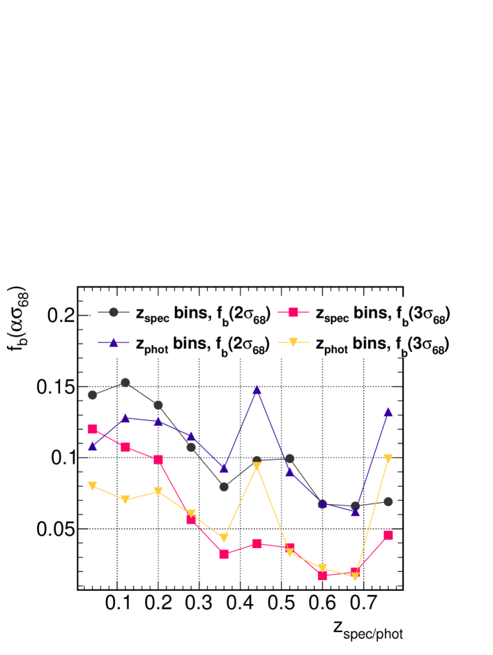
We observe a strong correlation between and . Fig. 5(b) - LABEL:sub@FIG_boss_singleANNmetrics3, show the photo- bias, scatter and outlier fractions as a function of the true and of the derived redshift values of ANNz2. All metrics exhibit worse performance at the edges of the redshift range, due in part to the relatively small number of respective training objects.
An additional important quantity which characterizes the performance of the code is the associated photo- uncertainty. For ANNz1, uncertainties were derived using a chain rule, propagating the uncertainties on the algorithm-inputs, to an uncertainty on the value of the final photo-. The disadvantage of such a scheme is that the uncertainty on photometric inputs, such as magnitudes, is not always precise in itself. This is due to the fact that in most cases, the available uncertainty estimation only represents the Poissonian noise on the corresponding photon-count. It therefore does not take into account other systematic uncertainties or correlations between observables.
In order to compute the uncertainty associated with our photo- estimator, denoted hereafter as , a data-driven method is employed. This is done by assuming that objects with similar combinations of photometric properties should also have similar photo- uncertainties. We derive the uncertainty using the K-nearest neighbours (KNN) method. We would emphasise that the latter should not be confused with K-nearest neighbours machine learning. For the calculation of , no additional training of an MLM is required. Rather, a simple search in parameter-space is performed.
For example, let us assume that magnitudes are used as inputs for training. In this case, the distance in parameter-space between a pair of galaxies, and , can be defined as
| (1) |
where the symbols stand for the five magnitudes, , , , and , for the two galaxies. The first step in the calculation is to find the nearest neighbours to our target object, defined as those with the smallest value of from the entire training sample. For each of the neighbours, we calculate the photo- bias. For neighbour , the latter is defined as , where is the estimated photo- of the objects, and is the respective spectroscopic redshift. The width of the distribution of values is then taken as the uncertainty on the photo- of the target object, .121212 In practice, we calculate the photo- uncertainty separately for shifts to lower or to higher values of redshift. However, for the sake of brevity, we refer to as symmetric in the following.
This technique has been shown to produce realistic photometric uncertainties, as e.g., in Oyaizu et al. (2008), so long as the training dataset is representative of the evaluated photometric sample. Additionally, the authors there discussed the optimal value for . It was explained that on the one hand, should be large enough that the uncertainty estimation is not limited by shot noise; on the other hand, should not be set too high, so that the estimate remains relatively local in the input parameter space. For the current study, a nominal value, , was selected.
We would like to assert that the uncertainty estimator represents the correct underlying photo- scatter in our analysis. For this purpose, we define the metric
| (2) |
the ratio between the photo- bias and the associated uncertainty. The distribution of the values of for the entire sample is expected to be centred close to zero, and to have a width close to unity.
The distributions of for our ANNz1 and ANNz2 solutions are shown in Fig. 6.
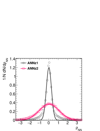
We proceed by fitting a Gaussian function to each dataset. We find that both distributions have a mean value which is consistent with zero to a precision better than . In addition, the distribution of for ANNz1 has a width of , while the corresponding value for ANNz2 is . This indicates that the uncertainty estimation for the ANNz2 photo-s is significantly more reliable in comparison.
4.3 Randomized regression PDF
As mentioned above, we construct our PDF by combining multiple MLM estimators, each folded with their respective single-value uncertainty estimator. The steps of the algorithm may be summarized as follows:
-
1.
A collection of MLMs is trained.
-
2.
The ensemble of estimators goes through pre-selection, which includes ranking the solutions by their performance. The MLM which performs best is chosen as the single-value estimator.
-
3.
The MLMs are folded with their corresponding intrinsic uncertainty, . They are then combined in different ways into a set of candidate-PDFs. The MLM combinations are chosen randomly, taking into account the ranking in performance.
-
4.
The performance of the candidates is compared, using the parameter , defined below. The solution which best describes the true redshift distribution is selected as the final PDF.
The first step in the calculation is the training of a set of randomized MLMs. These differ from each other in several ways. The latter includes setting unique random seed initializations, as well as changing the configuration parameters of a given algorithm.131313 See Sect. 5.1 and Appendix A for details. For instance, this may refer to using various types and numbers of neurons in an ANN, or to arranging neurons in different layouts of hidden layers; for BDTs, the number of trees and the type of boosting/bagging algorithm may be changed, etc.
In general, the choice of input parameters also has an effect on the performance (Hoyle et al., 2015b). A randomized MLM therefore has the option to only use a subset of the given input parameters, or to train with predefined functional combinations of parameters. These combinations may also incorporate complicated scenarios. For instance, missing inputs for a specific object may be mapped to predefined numerical values, such as the magnitude limits of the survey.
Additionally, TMVA provides the option to perform transformations on the input parameters, including normalization and principal component decomposition. The transformations are done prior to training, as part of the internal pipeline of the code. Applying transformations on inputs has the potential to improve the performance of machine learning. For instance, Soumagnac et al. (2015) used principal component analysis to augment their algorithm, by reducing the dimensionality of a classification task. For photo- inference, transformation are most useful when combining input observables of different types, such as magnitudes and surface brightness.
Finally, the user may define training weights using functional expressions of both input parameters and observer parameters (parameters not used directly for the training). The weights are applied during the training; they may e.g., be used to reduce the impact of noisy data on the result. These may come in addition to the weights meant to account for unrepresentative training datasets, which are discussed in the next section.
Once a set of randomized MLMs is initialized, the various methods are each trained. Subsequently, a distribution of photo- solutions for each galaxy is generated. A selection procedure is applied to the ensemble of answers, discarding outlier solutions which have very large values of , and , compared to the entire ensemble. The selected MLMs are then used to identify a single photo- estimator, based on the method with the best performance. The latter is denoted in the following as .
In the next step, the various MLMs are folded with their respective single-value uncertainty. They are then used in concert in order to derive a complete probability distribution function. The most trivial combination, is one in which we accept all MLMs with equal weights. This, however, does not necessarily result in the best outcome, as the inclusion of estimators with e.g., large scatter, degrades the performance. We therefore derive a dynamic weighting scheme for the combination of MLMs. The weights are determined, using the cumulative distribution function (CDF) of a candidate-PDF,
| (3) |
The latter is defined as the integrated PDF for redshifts smaller than some reference value, taken here as the true redshift, . Here the differential PDF for a given redshift is denoted by , and corresponds to the lower bound of the PDF.
Let us consider a photo- PDF which correctly describes the underlying redshift distribution. In this case, one may think of as a random variable which is distributed according to the PDF. It then follows that would be a flat distribution. As further illustration, one may imagine the inverse problem. Supposing we generate a collection of random numbers, uniformly distributed between 0 and 1. We then use these to calculate , the inverse of the CDF (the quantile function). In this case, the distribution of values would correspond to redshifts; it should then recover our PDF, assuming the PDF correctly represents the underlying uncertainty on our photo- inference.
The CDF of redshifts has previously been used to constrain photo- PDFs, as e.g., in Bordoloi et al. (2010). There it was the basis for modifying PDFs which were constructed from likelihood functions, as part of a template fitting algorithm. In ANNz2, is used for the initial derivation procedure of the PDF. This is done by selecting from the collection of candidate-PDFs, the solution for which is as close as possible to a uniform distribution.
4.4 Representativeness and completeness of the training sample
Up to this point, we have discussed how the uncertainty on input parameters and the differences between specific MLMs are treated in ANNz2. However, machine learning methods based on training are susceptible to additional systematic effects. Two possible sources of major bias come about for training datasets which are not representative or are not complete.
One possible source of bias is the exact composition of the training dataset. Let us consider an evaluated object from a photometric dataset, for which we have comparable training objects. It is then important that the relative fraction of these training objects within the training sample be the same as in the photometric dataset. If this is not the case, the training sample is usually referred to as unrepresentative.
In order to illustrate the point, a simple example is shown in Fig. 7. The figure includes the distributions of the r-band magnitude, , of objects in hypothetical training and reference samples. The latter represents a complete and unbiased representation of the of galaxies for some survey. In this case, the distribution of in the training dataset is quite different from that in the reference sample. An MLM trained using this training dataset will e.g., give too high significance to training examples with values close to .
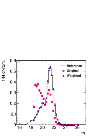
The problem may be alleviated by reweighting the training sample. The purpose of the weights is to assign a correction factor to galaxies as a function of the input parameters. The weighted distribution of galaxies should be such, that the relative fraction of objects in each region in the parameter space is the same as in the reference sample. These weights are then used as part of the training; they are also further propagated to the metric calculations, to be used during the PDF optimization phase. The reweighting procedure is implemented as part of the internal pipeline of ANNz2, requiring only the definition of the reference dataset by the user of the code.
The weights are derived by matching the density of objects in the input parameter space to that in the reference sample (Lima et al., 2008). This way, all inputs are reweighted simultaneously, accounting for any intrinsic correlations. We derive the weights using a kd-tree, calculating the number of neighbours of an object in the training sample within some distance (see Equations 1). We then find the number of neighbours of the same object within the same distance, but in the reference sample. The weight is finally taken as the ratio of these two numbers.
One may notice in Fig. 7 that for , the weighted training dataset does not match the reference sample. The reason for this, is that the original training sample does not have any corresponding objects. In this case, we usually refer to the training dataset as incomplete. In general, an MLM should only be used on objects which have features that are represented in the training dataset. In cases where no training examples exist, both the photo- and the corresponding photo- uncertainty are equally unreliable.
ANNz2 has a validation mechanism to check whether an evaluated object falls under an incomplete region of the training sample. Unfortunately, there is no systematic way to correct the photo- of objects which do not have comparable training examples. These can instead be flagged as unreliable.
The algorithm uses a kd-tree to derive the density of objects from the training sample, which have similar properties as the evaluated object. We begin by computing , the distance in parameter-space between the evaluated object, , and the closest corresponding object from the training sample, (see Equations 1). We then derive , the distance from , within which objects from the training sample are found. Finally, we define our quality criteria as
| (4) |

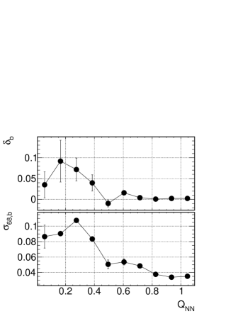
The parameter represents a typical distance-ratio between the evaluated object, and similar training objects. For dense regions of the training sample, , which corresponds to . Conversely, for sparse regions, one would have to search far away in order to find object-, resulting in low values of . The steepness of the distribution of depends on the choice of , and on the properties of the dataset. We nominally use , though this parameter may be changed by the user of the code.
The parameter can be used to reject low-fidelity photo-s. The exact cut on should be determined on a case-by-case basis. It should take into account the fraction of excluded objects, and the relative improvement in performance. To illustrate the properties of , we use the hypothetical training and reference samples defined for Fig. 7. For the purpose of the example, we take the reference sample as the evaluated dataset. The corresponding distribution of values is presented in Fig. 8(a). We quantify our results in Fig. 8(b). Here, we present the dependence on of the photo- bias, , and of the scatter, . As desired, the performance improves as the value of increases. For this example, a conservative cut would be to reject galaxies with .
5 Performance of the estimators of ANNz2
5.1 Toy analysis
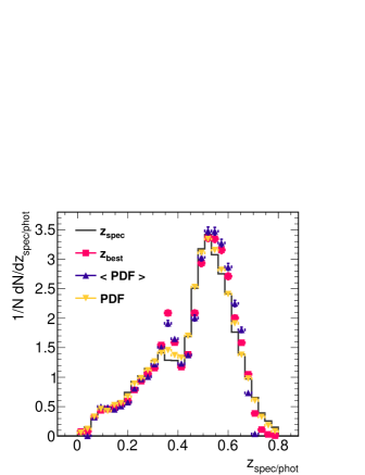
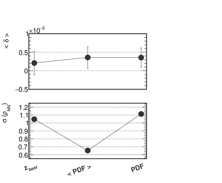
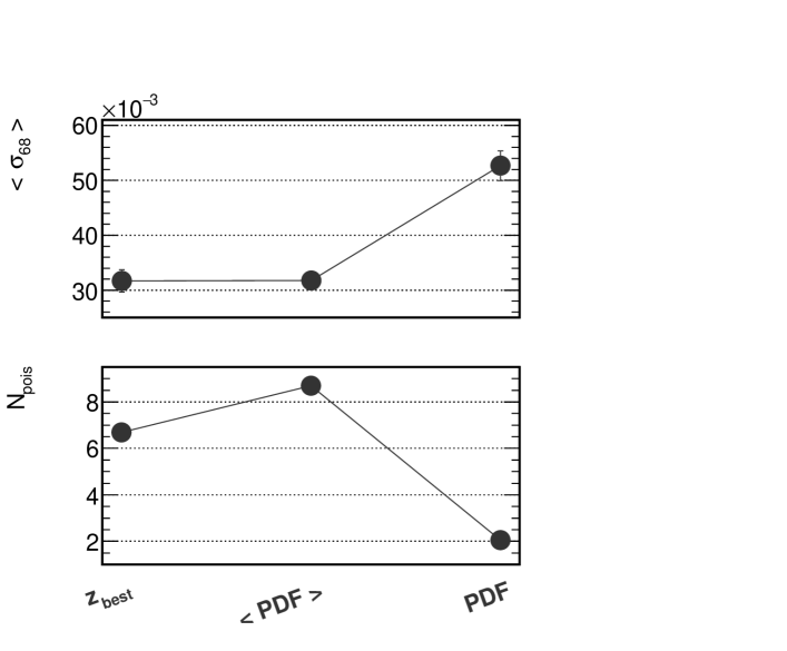
Figure 9 shows the distribution of the nominal photo- estimators of ANNz2 for our SDSS dataset. These include the single-value photo- estimator, , the single-value average of the randomized regression PDF, , and the full PDF solution, .
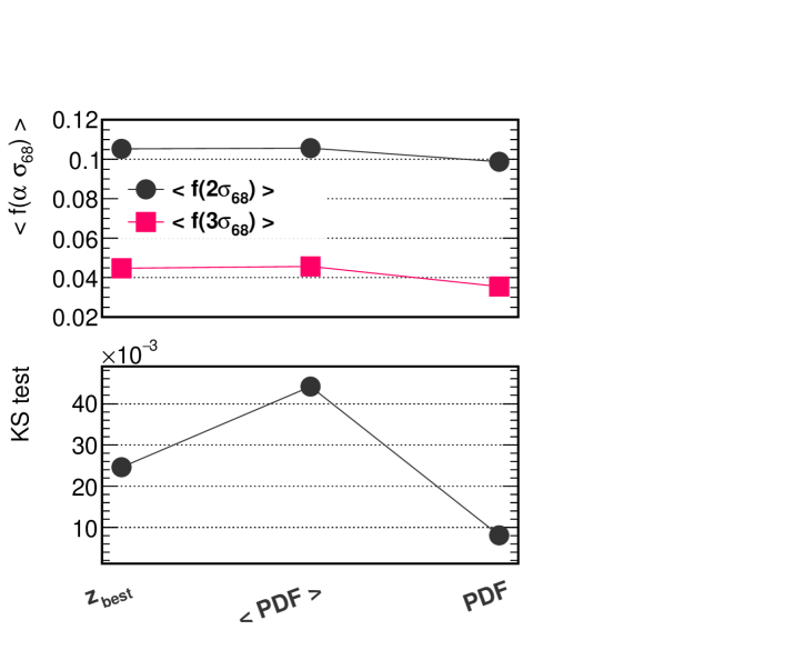
The corresponding performance metrics are presented in Fig. 10; the bias, ; the scatter, ; and the outlier fractions, and . In addition, we include the metric , defined as the width of the distribution of (see Equations 2). Finally, the and -test statistics of the various distributions are shown as well.
The solution is the same one shown in Fig. 5, and corresponds to an ANN with architecture , where corresponds to the number of input parameters (in this case, five magnitudes). The ensemble of MLMs used for the PDF is composed of 50 ANNs and 50 BDTs, with specific MLM options chosen at random as described next. In addition, for both the ANNs and the BDTs, the input parameters for the training were chosen as either the five magnitudes, combinations of magnitude and colours, or subsets of the latter. Furthermore, variable transformations on the input parameters (normalization, principal component analysis, decorrelation) were switched on or off at random.
The ANNs were configured with variations of the following parameters:141414 See Appendix A for details on the configuration options. the numbers of hidden layers was varied between 2 and 4; the number of neurons in a hidden layer was varied between and ; the neuron activation function was chosen as either a sigmoid or a tanh function; use of a regulator was switched on or off; the number of steps between convergence tests was randomized between 100 and 500 steps; the MLMs were trained using back-propagation, with or without the use of second derivatives of the ANN error function.
The BDTs were defined using the following settings: the number of trees was randomized between 300 and 1200; the boosting algorithm was changed between the available options in TMVA; the threshold criteria for splitting nodes was varied between and of the number of training objects per node; the separation criteria for testing node-splitting was chosen at random.
We observe that the three photo- estimators, , and , all have an average bias which is consistent with zero. Comparing the scatter, the full PDF has a larger scatter relative to the single-value estimators. This is expected, as the calculation for PDFs is performed bin-by-bin, taking into account the tails of the PDF. For approximately symmetric PDFs, the tails cancel out. They therefore do not affect the bias or scatter of the average of the PDF. However, for the full solution, the negative and positive contributions from the tails increase . The scatter for the full PDF is therefore larger by construction. The increased value of the PDF scatter is not a disadvantage. Rather, it represents a more realistic estimation of the underlying uncertainty on the photo-s. This is reflected by the value of , which is much better (closer to 1) for the estimator, than for its average.
Finally, the shape of the full PDF provides a better description of the underlying redshift distribution, as expressed by the low values of the and -test statistics. The difference in the performance may even be appreciated by eye from Figure 9. Specifically, the stacked provides a better estimation of the true redshift for and for , where the single-value solutions are less precise.
5.2 Other applications of ANNz2
We have only commented here on performance metrics for ANNz2, such as photo- bias, and compatibility with the underlying redshift distribution. However, to fully qualify the algorithm, one would need to perform a Cosmological analysis involving photometric redshifts (Rau et al., 2015). Such a study is beyond the scope of the current work. However, ANNz2 has already been used for several DES analyses, and is included in the first public data release of the experiment.
In Bonnett et al. (2015), the performance of ANNz2 was compared with that of three other codes, SkyNet, TPZ and BPZ. The first two are machine-learning codes which employ a similar algorithm using different MLM types, while BPZ is a template-fitting code. The comparison was done in the context of the first DES Cosmology results (DES Collaboration, 2015), where the difference between the photo-s were propagated to the systematic uncertainty on a weak lensing analysis. One should notice that Bonnett et al. (2015) performed the comparison between the different estimators by first assigning galaxies to one set of redshift bins. The latter were determined by the nominal code in the study, SkyNet. The photo-s of the various codes for a given galaxy sub-sample (SkyNet photo- bin) were then compared. This may produce a selection bias; effectively, the PDF for each code is constrained by the results of SkyNet. However, even given this possible bias, ANNz2 was found to be compatible with the other codes.
In another study (Leistedt et al., 2015), a systematic test of variations in the observing conditions in DES was performed, comparing ANNz2, TPZ and BPZ. In this case, it was shown that ANNz2 minimizes the variations in the photo- distribution due to degraded input data, and that it reduces the amount of outliers.
6 Summary
ANNz2 is a new major version of the public photometric redshift estimation software, first developed by Collister and Lahav (2004). It has already been used as part of the first weak lensing analysis of the Dark Energy Survey, and is included in the first data release of the experiment. The code is also planned to be incorporated in the software pipelines of future projects. In this paper we have introduced the algorithm available in the new implementation, and have illustrated the performance of the code using spectroscopic data.
ANNz2 incorporates several machine learning methods, such as artificial neural networks and boosted decision/regression trees. The different algorithms are used in concert in order to optimize the photo- reconstruction, and to estimate the associated uncertainties. This is done by generating a wide selection of machine learning methods, utilizing e.g., different ANN architectures and BDT algorithms. The final product of ANNz2 is either a single-value photo- estimator, or a full photo- probability distribution function. PDF derivation is an important new feature of ANNz2, not available in the previous version of the code.
PDFs are calculated by ANNz2 using two different approaches. The nominal approach is a new technique, called randomized regression. In this mode, optimization is performed by ranking the different solutions according to their performance, which is determined by the respective photo- bias, scatter and outlier fraction parameters. The single solution with the best performance is chosen as the nominal photo- estimator of ANNz2. In addition, the entire collection of solutions is used in order to derive a photo- PDF. The PDF is constructed in two phases. In the first phase, each solution is folded with a distribution of uncertainty values, which is derived using the KNN uncertainty estimation method. In the second phase, the ensemble of solutions is combined. This is done using dynamically determined weighting schemes, intended to optimize the final PDF. Additionally, we have implemented in ANNz2 a second approach for PDF-derivation, called binned classification. The latter has been used in the past, and is not discussed in the current paper.
ANNz2 also includes an implementation of a method to correct for training samples which are not representative of the features of the evaluated dataset. In addition, we introduce a new method to account for samples which are not complete. The former is performed by applying weights to training objects during training and during photo- optimization, in order to match the properties of the evaluated dataset. For the latter, a quality flag is generated for each evaluated object. The flag indicates whether the derived photo- solution is reliable, based on the completeness of the sample.
Acknowledgements
We would like to thank Manda Banerji, Christopher Bonnett, Antonella Palmese and Maayane Soumagnac for the useful discussions regarding the nature of photometric redshifts and machine learning. We would also like to thank the photo- working groups of DES and of the Euclid experiment for giving feedback on the code.
OL acknowledges an European Research Council Advanced Grant FP7/291329, which also supported IS. FBA acknowledges the Royal Society for a Royal Society University Research Fellowship.
This work uses publicly available data from the SDSS. Funding for SDSS-III has been provided by the Alfred P. Sloan Foundation, the Participating Institutions, the National Science Foundation, and the U.S. Department of Energy Office of Science. The SDSS-III website is http://www.sdss3.org/.
References
- Abdalla et al. (2008) Abdalla, F. B., Amara, A., Capak, P., et al.: 2008, MNRAS 387, 969
- Abdalla et al. (2011) Abdalla, F. B., Banerji, M., Lahav, O., and Rashkov, V.: 2011, MNRAS 417, 1891
- Ahn et al. (2014) Ahn, C. P., Alexandroff, R., Allende Prieto, C., et al.: 2014, ApJS 211, 17
- Arnouts et al. (1999) Arnouts, S., Cristiani, S., Moscardini, L., et al.: 1999, MNRAS 310, 540
- Banerji et al. (2008) Banerji, M., Abdalla, F. B., Lahav, O., and Lin, H.: 2008, MNRAS 386, 1219
- Benitez (2000) Benitez, N.: 2000, ApJ 536, 571
- Benítez et al. (2009) Benítez, N., Moles, M., Aguerri, J. A. L., et al.: 2009, ApJ 692, L5
- Bolzonella et al. (2000) Bolzonella, M., Miralles, J.-M., and Pelló, R.: 2000, A&A 363, 476
- Bonnett (2015) Bonnett, C.: 2015, MNRAS 449(1), 1043
- Bonnett et al. (2015) Bonnett, C., Troxel, M. A., Hartley, W., et al.: 2015, ArXiv e-prints
- Bordoloi et al. (2010) Bordoloi, R., Lilly, S. J., and Amara, A.: 2010, MNRAS 406(2), 881
- Brun and Rademakers (1997) Brun, R. and Rademakers, F.: 1997, Nucl.Instrum.Meth. A389, 81
- Bruzual A. and Charlot (1993) Bruzual A., G. and Charlot, S.: 1993, ApJ 405, 538
- Carrasco Kind and Brunner (2013) Carrasco Kind, M. and Brunner, R. J.: 2013, MNRAS 432, 1483
- Carrasco Kind and Brunner (2014) Carrasco Kind, M. and Brunner, R. J.: 2014, MNRAS 438, 3409
- Coleman et al. (1980) Coleman, G. D., Wu, C.-C., and Weedman, D. W.: 1980, ApJS 43, 393
- Collister and Lahav (2004) Collister, A. A. and Lahav, O.: 2004, PASP 116, 345
- Connolly et al. (1995) Connolly, A. J., Csabai, I., Szalay, A. S., et al.: 1995, AJ 110, 2655
- Dawson et al. (2013) Dawson, K. S., Schlegel, D. J., Ahn, C. P., et al.: 2013, AJ 145, 10
- DES Collaboration (2015) DES Collaboration: 2015, ArXiv:1507.05552
- Feldmann et al. (2006) Feldmann, R., Carollo, C. M., Porciani, C., et al.: 2006, MNRAS 372, 565
- Firth et al. (2003) Firth, A. E., Lahav, O., and Somerville, R. S.: 2003, MNRAS 339, 1195
- Geach (2012) Geach, J. E.: 2012, MNRAS 419, 2633
- Gerdes et al. (2010) Gerdes, D. W., Sypniewski, A. J., McKay, T. A., et al.: 2010, ApJ 715, 823
- Hastie et al. (2001) Hastie, T., Tibshirani, R., and Friedman, J.: 2001, The Elements of Statistical Learning, Springer Series in Statistics, Springer New York Inc., New York, NY, USA
- Hildebrandt et al. (2010) Hildebrandt, H., Arnouts, S., Capak, P., et al.: 2010, A&A 523, A31
- Hoecker et al. (2007) Hoecker, A., Speckmayer, P., Stelzer, J., et al.: 2007, PoS ACAT, 040
- Hoyle et al. (2015a) Hoyle, B., Rau, M. M., Bonnett, C., Seitz, S., and Weller, J.: 2015a, MNRAS 450, 305
- Hoyle et al. (2015b) Hoyle, B., Rau, M. M., Zitlau, R., Seitz, S., and Weller, J.: 2015b, MNRAS 449, 1275
- Hu (1999) Hu, W.: 1999, ApJ 522, L21
- Ilbert et al. (2006) Ilbert, O., Arnouts, S., McCracken, H. J., et al.: 2006, A&A 457, 841
- Leistedt et al. (2015) Leistedt, B., Peiris, H. V., Elsner, F., et al.: 2015, ArXiv e-prints
- Lima et al. (2008) Lima, M., Cunha, C. E., Oyaizu, H., et al.: 2008, MNRAS 390, 118
- MacKay (2003) MacKay, D. J.: 2003, Information theory, inference and learning algorithms, Cambridge university press
- Mandelbaum et al. (2008) Mandelbaum, R., Seljak, U., Hirata, C. M., et al.: 2008, MNRAS 386, 781
- Mobasher et al. (2007) Mobasher, B., Capak, P., Scoville, N. Z., et al.: 2007, Astrophys. J. Suppl. 172, 117
- Myers et al. (2009) Myers, A. D., White, M., and Ball, N. M.: 2009, MNRAS 399, 2279
- Newman et al. (2015) Newman, J. A., Abate, A., Abdalla, F. B., et al.: 2015, Astropart. Phys. 63, 81, [Erratum: Astropart. Phys.65,112(2015)]
- Oyaizu et al. (2008) Oyaizu, H., Lima, M., Cunha, C. E., Lin, H., and Frieman, J.: 2008, ApJ 689, 709
- Rau et al. (2015) Rau, M. M., Seitz, S., Brimioulle, F., et al.: 2015, MNRAS 452(4), 3710
- Sánchez et al. (2014) Sánchez, C., Carrasco Kind, M., Lin, H., et al.: 2014, MNRAS 445, 1482
- Schmidt (2007) Schmidt, S.: 2007, Galaxy Evolution: The DRaGONS Survey and Luminosity Functions with Photometric Redshifts, University of Pittsburgh
- Soumagnac et al. (2015) Soumagnac, M. T., Abdalla, F. B., Lahav, O., et al.: 2015, MNRAS 450(1), 666
- Way and Klose (2012) Way, M. J. and Klose, C. D.: 2012, PASP 124, 274
- Zhan and Knox (2006) Zhan, H. and Knox, L.: 2006, ArXiv Astrophysics e-prints
Appendix
Appendix A Quick-start guide
To illustrate the use of ANNz2, we provide a short guide for running the code. The following is limited to describing the randomized regression mode, corresponding to version 2.1.2 of the code. Please see the on-line documentation151515 See https://github.com/IftachSadeh/ANNZ . for further details, as well as up to date instructions.
A.1 Work-flow
Randomized regression is run using the following consecutive shell commands. In this example, the commands employ the Python control script, annz_rndReg_quick.py, which is provided with the code:
These correspond to the four stages of the pipeline: data processing, training, optimization, and evaluation.
In the following, we describe each of these stages. We use Python pseudo-code to represent the content of the example script. The dictionary syntax, ANNz[”XXX”], stands for a job-option parameter labelled XXX, which is exposed to ANNz2. All other variables are internal to the control script.
A.2 Data processing
In the initial stage, the training and validation samples defined by the user are ingested. If the user does not explicitly define separate input files for training and for validation, the complete sample is randomly split.
The user also has the option to define a reference sample, which represents the dataset which is eventually evaluated. If this reference is provided, training weights are calculated, as described in Sect. 4.4.
For example, the user may define,
Here inAsciiFiles defines the input file containing the dataset for training and validation. The corresponding list of variables in this file is defined in inAsciiVars. For brevity, we define only a few inputs here; these are formatted as a semicolon-separated list of variable type and name. The former are e.g., F, standing for floating precision, D, standing for double precision, and C, standing for a string variable. The variable names, m_u, e_u, m_g and e_g stand in this example for a pair of magnitudes and their corresponding errors; the variable z_spec stands for the spectroscopic redshift; the variable survey stands for the name of the spectroscopic survey. We note that our use of magnitudes, while useful for photo- estimation, has no particular significance. The user may assign any type of input (with any assigned name) as part of the input dataset.
Setting the variable useWgtKNN to True activates the calculation of training weights. The associated parameters are inAsciiFiles_wgtKNN and inAsciiVars_wgtKNN, respectively used to define the file-name of the reference sample, and the corresponding list of variables it contains. The parameter, weightVarNames_wgtKNN defines the variables which are used for the KNN search. In this example, distance between neighbours is defined in magnitude (m_u, m_g), in magnitude-error (e_u, e_g) and in colour (m_u-m_g). Any functional combination of input parameters may be used for the KNN search, for any variable which is defined in both inAsciiVars and inAsciiVars_wgtKNN.
Once training weights are calculated, they are propagated automatically to all calculations in the following stages. This includes the training of MLMs, the optimization process and the performance plots generated as part of the output of the code. The training weights themselves are also included as part of the output of ANNz2, for every object from the training and validation samples. ANNz2 may thus also be used to calculate representativeness weights for use by other codes.
A.3 Training
In the second stage of the pipeline, a collection of MLMs is trained. The MLMs may be trained consecutively, or in parallel (e.g., using a batch-system).
For example, the user may set the following options:
The target of the regression (the spectroscopic redshift) is defined in zTrg, with the allowed limits for the latter set in minValZ and maxValZ. In this case, randomized MLMs will be trained (specified by nMLMs). The variables used as input for the training are defined in inputVariables. One can select any functional combination of the available parameters which have previously been defined in inAsciiVars, including logical expressions. An example for the latter is the choice made for the third option. Here magnitudes are mapped to some effective magnitude-limit, which may prevent training with noisy data.
The type of MLM for each of the randomized ensemble is defined in the userMLMopts parameter. The current example shows configurations of an ANN, a BDT and a KNN. Here, the ANN is defined as having two hidden layers, the first with N and the second with N+5 neurons, where N is the number of input parameters; the selected type of neuron is a sigmoid function; a regulator is used for the training; the training method is chosen as BFGS (using second derivatives of the error function); a maximum of training cycles are allowed. The BDT is defined as being composed of trees (NTrees); a minimum of of training objects is included in each tree-node (MinNodeSize); training employs the AdaBoost boosting algorithm (BoostType). The KNN in this example is defined simply as using near neighbours.
Of the key-words defined for userMLMopts, the only pattern unique to ANNz2 is (ANNZ_MLM = XXX), here with XXX being ANN, BDT or KNN. This tag defines for ANNz2 which MLM type to use. All other job-options are native to TMVA. For instance, an ANN may be trained with TrainingMethod = BP, GA, or BFGS; a BDT may use boosting (BoostType = AdaBoost, RealAdaBoost, AdaBoostR2, or Grad), or it may use bagging (ABaggingNN), etc. The various possible settings are defined in the TMVA manual,161616 See http://tmva.sourceforge.net/optionRef.html . along with overviews of the corresponding algorithms. All machine learning methods available through TMVA may be used in ANNz2. However, in our experience, ANNs and BDTs perform best for the task of photo- inference.
In the current example, the user has also requested that the variables used for training the BDT will have gone through transformations prior to training. The latter are defined using the VarTransform parameter, with N representing normalization, D, decorrelation, and P standing for principle-component decomposition. The VarTransform flag may be added to any userMLMopts option string, for any type of MLM. The transformations are performed as part of the internal pipeline of the code, and are automatically applied to evaluated objects.
The empty selection for userMLMopts indicates for ANNz2 that MLM configuration parameters should be chosen on the fly. This is done as part of the internal pipeline of the code, and results in randomized configurations of ANNs and BDTs.
In the example, we also show how the user may define cuts for the training and validation samples (userCuts_train, userCuts_valid). For instance, assuming we have spectroscopic data from several surveys, the user has chosen to only train with galaxies from the ”SDSS” survey. In addition, a cut is set to only use objects with e_u below certain limits. Such choices are useful for comparing the performance for different training sub-samples. Additionally, weights may be defined for the training and validation samples using userWeights_train and userWeights_valid. These take effect in addition to the representativeness weights, provided the latter were calculated in the previous stage. We note that the various cut and weight expressions can be set to different values for each of the randomized MLMs. For instance, the user may choose to impose a cut on magnitude errors for half of the randomized MLMs, to asses if such a constraint improves the performance or not.
A.4 Optimization
In the optimization stage, the performance of the ensemble of trained MLMs is derived. The optimal solution is chosen as , and a PDF is derived.
There are several control options which the user may set,
The first block shows how the user may define the binning-scheme for the PDFs. One may set one of the following: userPdfBins can be used to define a specific set of bins; nPDFbins can be used to divide the allowed range of the regression target into (in this case) bins of equal width; pdfBinWidth can be used to divide the allowed range into a dynamically determined number of bins, which all have a width of (in this case) .
In general, all derived MLMs are combined to form the PDF. However, it is possible to set exclusion criteria, and reject those which perform badly. The parameters max_bias_PDF, max_sigma68_PDF and max_frac68_PDF represent these criteria; these respectively define upper limits on the values of the bias, the scatter, and corresponding combined outlier fraction. Individual MLMs with metric values higher than the upper limits, are not incorporated into the PDF.
By default, only and the PDF are included in the output of ANNz2. However, it is possible for the user to define additional MLM estimators to be written out. This is done using the MLMsToStore parameter, which may include any MLM-id in the range, .
A.5 Evaluation
In the final stage of the pipeline, the user defines a dataset, for which the photo- estimators are calculated. Additionally, the quality parameter for incomplete training, , can be calculated on request.
For example, it is possible to choose the following configuration:
where the inAsciiFiles and inAsciiVars variables are set as for the initial data processing stage. We note that inAsciiVars does not need to exactly correspond to the same structure as for the previous stages. However, it must include all variables which were used for training MLMs (see inputVariables).
If the addInTrainFlag parameter is set to True, the estimator is added to the output. For the calculation of , the user needs to define weightVarNames_inTrain, the list of variables to be used for the KNN search. The user also has the option to set the value of (see Sect. 4.4), using the parameter, minNobjInVol_inTrain.