, , ,

Distribution of the position of a driven tracer in a hardcore lattice gas

Pierre Illien, Olivier Bénichou, Gleb Oshanin and Raphaël Voituriez Université Pierre-et-Marie-Curie (Paris 6) - Laboratoire de Physique Théorique de la Matière Condensée (UMR CNRS 7600), 4 place Jussieu, 75005 Paris, France illien@lptmc.jussieu.fr benichou@lptmc.jussieu.fr oshanin@lptmc.jussieu.fr voiturie@lptmc.jussieu.fr
Abstract

We study the position of a biased tracer particle (TP) in a bath of hardcore particles moving on a lattice of arbitrary dimension and in contact with a reservoir. Starting from the master equation satisfied by the joint probability of the TP position and the bath configuration and resorting to a mean-field-type approximation, we presented a computation of the fluctuations of the TP position in a previous publication [Phys. Rev. E 87, 032164 (2013)]. Counterintuitively, on a one-dimensional lattice, the diffusion coefficient of the TP was shown to be a non-monotonic function of the density of bath particles, and reaches a maximum for a nonzero value of the density. Here, we: (i) give the details of this computation and offer a physical insight into the understanding of the non-monotonicity of the diffusion coefficient; (ii) extend the mean-field-type approximation to decouple higher-order correlation functions, and obtain the evolution equation satisfied by the cumulant generating function of the position of the TP, valid in any space dimension. In the particular case of a one-dimensional lattice, we solve this equation and obtain the probability distribution of the TP position. We show that the position rescaled by its fluctuations is asymptotically distributed accordingly to a Gaussian distribution in the long-time limit.

1 Introduction

1.1 Context

Studying the dynamics of an active particle or a particle submitted to an external force travelling in a crowded environment is a frequent problem in physics and in biology. Different examples are found in biophysics, when one considers molecular motors, motile living cells or bacteria [1, 2], or in the study of biased intruders in granular systems [3] or colloidal suspensions [4]. The determination of the dynamics of this tracer particle (TP) is consequently an important question, with different applications. In particular, new experimental tools allow the study of a medium using a microscopic probe particle submitted to an external force. This field of research, commonly named active microrheology, has been applied to different systems in the past decades, among which biological cells [5, 6], complex fluids [7, 8] and colloidal suspensions [4, 9].

From a theoretical point of view, the difficulty lies in the modeling of the environment of the tracer particle (TP), which is constituted of a large number of interacting bath particles. In most analytical approaches, the evolution of the position of the TP is studied with some effective description of the bath of particles [10], which do not take into account the correlations between the position of the TP and the density profiles of the surrounding bath. In the situation where the TP and the bath particles have comparable sizes, the response of the probe to the external forcing, and in particular its fluctuations, cannot be accounted for correctly with an effective treatment.

Here, we study the diffusion of a driven tracer in a lattice gas of hardcore particles. This minimal model explicitly takes into account the bath dynamics: the driven TP performs a biased nearest-neighbor random walk, in a bath of particles performing symmetric nearest-neighbor random walks, with the restriction that each site is occupied by at most one particle. We assume that the lattice is in contact with a reservoir of particles, so that the bath particles present on the lattice may desorb back to the reservoir, and particles from the reservoir may adsorb onto vacant lattice sites. This so-called Langmuir kinetics is relevant to describe situations where a gas or a vapor is brought in contact with a solid surface, on which the gas particles may form an adsorbed layer. The transport properties of the adsorbed particles have been shown to control many different processes, such as spreading of molecular films on solid surfaces [11] or dewetting [12, 13]. The particular case where the Langmuir kinetics is coupled to a Totally Asymmetric Exclusion Process was investigated theoretically [14, 15], and has been show to be relevant to describe the directional motion of molecular motors on a cytoskeletal filament, with random attachment and detachment of the motors [16, 17].

Studying the transport properties of a biased TP in a hardcore lattice gas is actually a complex N𝑁N-body problem. In the situation where the density of bath particles ρ𝜌\rho is very high and where the number of particles on the lattice is conserved, the problem can be treated exactly to obtain results at leading order in (1ρ)1𝜌(1-\rho) [18, 19, 20, 21]. For an arbitrary density of particles, exact results were established concerning the mean position of the TP in the one-dimensional situation [22], and concerning the validity of the Einstein relation [23]. The situation where the lattice is populated by an arbitrary density of particles and where it is in contact with a reservoir of particles was addressed by resorting to a mean-field-type approximation consisting of the decoupling of relevant correlation functions, allowing the computation of the mean position of the TP and of the bath density profiles in the long-time limit, in the case of a one-dimensional lattice [24] and for lattices of higher dimension [25, 26, 27, 28]. Numerical simulations sampling exactly the master equation of the problem revealed the accuracy of the decoupling approximation in a wide range of parameters. The situation where the bath particles are fixed and can appear and disappear with prescribed rates, known as dynamical percolation [29], was also considered [30].

More recently, by extending the decoupling approximation initially proposed to study the mean position of the TP, its fluctuations have been studied [31]. An evolution equation for the fluctuations of the TP on a lattice of arbitrary dimension was obtained. This equation was solved explicitly in the case of a one-dimensional lattice, and in the stationary limit. The analysis of the solutions revealed a striking feature of the diffusion coefficient: in a wide range of parameters, it is shown to be a nonmonotonic function of the density of particles on the lattice. Counterintuitively, the diffusion coefficient of the TP can then be enhanced by the presence of bath particles in its environment.

Recently, this nonmonotonicity was also observed in the situation where the TP is dragged in a bath of soft particles [32, 33], and then appears to be a generic feature of biased intruders in crowded environments.

1.2 Main results of this paper and overview

In this paper, we first give a detailed computation of the results presented in [31]: we establish the evolution equation of the fluctuations of the TP position in arbitrary dimension under the decoupling approximation, and solve it in the case of a one-dimensional lattice. We show that the non-monotonicity of the diffusion coefficient with respect to the density of particles on the lattice is correlated to a non-monotonicity of some cross-correlation functions with respect to the distance to the TP.

The main result of this paper is the following: we go one step further and generalize the mean-field-type approximation in order to calculate the cumulant generating function of the position of the TP, and therefore its complete probability distribution. Denoting by 𝑿tsubscript𝑿𝑡\boldsymbol{X}_{t} the position of the TP, by Xt=𝑿t𝒆1subscript𝑋𝑡subscript𝑿𝑡subscript𝒆1X_{t}=\boldsymbol{X}_{t}\cdot\boldsymbol{e}_{1} its projection along the direction of the bias, and defining the cumulant generating function Ψ(u;t)lneiuXtΨ𝑢𝑡superscriptei𝑢subscript𝑋𝑡\Psi(u;t)\equiv\ln\langle\mathrm{e}^{\mathrm{i}uX_{t}}\rangle, we obtain in the long-time limit

Ψ(u;t)tΦ(u)t,Ψ𝑢𝑡𝑡similar-toΦ𝑢𝑡\Psi(u;t)\underset{t\to\infty}{\sim}\Phi(u)t, (1)

with

Φ(u)=p1τ(eiuσ1)[1eiuXtη𝑿t+𝒆1eiuXt]+p1τ(eiuσ1)[1eiuXtη𝑿t𝒆1eiuXt],Φ𝑢subscript𝑝1𝜏superscriptei𝑢𝜎1delimited-[]1delimited-⟨⟩superscriptei𝑢subscript𝑋𝑡subscript𝜂subscript𝑿𝑡subscript𝒆1delimited-⟨⟩superscriptei𝑢subscript𝑋𝑡subscript𝑝1𝜏superscriptei𝑢𝜎1delimited-[]1delimited-⟨⟩superscriptei𝑢subscript𝑋𝑡subscript𝜂subscript𝑿𝑡subscript𝒆1delimited-⟨⟩superscriptei𝑢subscript𝑋𝑡\Phi(u)=\frac{p_{1}}{\tau}\left(\mathrm{e}^{\mathrm{i}u\sigma}-1\right)\left[1-\frac{\left\langle\mathrm{e}^{\mathrm{i}uX_{t}}\eta_{\boldsymbol{X}_{t}+\boldsymbol{e}_{1}}\right\rangle}{\left\langle\mathrm{e}^{\mathrm{i}uX_{t}}\right\rangle}\right]+\frac{p_{-1}}{\tau}\left(\mathrm{e}^{-\mathrm{i}u\sigma}-1\right)\left[1-\frac{\left\langle\mathrm{e}^{\mathrm{i}uX_{t}}\eta_{\boldsymbol{X}_{t}-\boldsymbol{e}_{1}}\right\rangle}{\left\langle\mathrm{e}^{\mathrm{i}uX_{t}}\right\rangle}\right], (2)

where pνsubscript𝑝𝜈p_{\nu} is the jump probability of the TP in the direction ν𝜈\nu of the lattice, τ𝜏\tau is its characteristic jump time, σ𝜎\sigma is the lattice spacing and η𝒓subscript𝜂𝒓\eta_{\boldsymbol{r}} is the occupation number at site 𝒓𝒓\boldsymbol{r}. The evolution equations for the correlation functions w~𝒓(u;t)=eiuXtη𝑿t+𝒓/eiuXtsubscript~𝑤𝒓𝑢𝑡delimited-⟨⟩superscriptei𝑢subscript𝑋𝑡subscript𝜂subscript𝑿𝑡𝒓delimited-⟨⟩superscriptei𝑢subscript𝑋𝑡\widetilde{w}_{\boldsymbol{r}}(u;t)={\left\langle\mathrm{e}^{\mathrm{i}uX_{t}}\eta_{\boldsymbol{X}_{t}+\boldsymbol{r}}\right\rangle}/{\left\langle\mathrm{e}^{\mathrm{i}uX_{t}}\right\rangle} are obtained using an extension of the mean-field-type approximation proposed to study the mean and fluctuations of the position of the TP. This result is given by Eqs. (74) and (75), where the quantities k𝒓(t)=η𝑿t+𝒓subscript𝑘𝒓𝑡delimited-⟨⟩subscript𝜂subscript𝑿𝑡𝒓k_{\boldsymbol{r}}(t)=\left\langle\eta_{\boldsymbol{X}_{t}+\boldsymbol{r}}\right\rangle are the density profiles in the reference frame of the TP and are the solutions of Eqs. (15) and (16). The equations satisfied by the correlation functions w~𝒓(u;t)subscript~𝑤𝒓𝑢𝑡\widetilde{w}_{\boldsymbol{r}}(u;t) are solved in the particular case of a one-dimensional lattice, and we compute the probability distribution of the position of the TP. We show that all the cumulants of the TP position scale as t𝑡t.

We also consider the random variable obtained by rescaling the position of the TP by t𝑡\sqrt{t}. For this random variable, all the cumulants of order greater than 222 vanish in the long-time limit, which shows that the position of the TP is asymptotically Gaussian.

The article is organized as follows. In section 2, we present the model and give the master equation governing the joint probability of the position of the TP and of the bath particles configuration. In section 3, we give the evolution equations of the first two cumulants. These equations involve the density profiles around the TP and some tracer-bath cross-correlation functions, whose evolution equations are explicitly given in a closed form by resorting to a mean-field-type approximation. In section 4, we generalize this approximation in order to obtain a closed set of equations for the cumulant generating function of the TP position. These equations are valid in arbitrary dimension, and they give in principle the whole probability distribution of the TP position. As a particular case, we also obtain the equation satisfied by the third-cumulant of the distribution. In section 5, we solve the equations obtained under the decoupling approximation in the particular case of a one-dimensional lattice, and then obtain explicit expressions for the first three cumulants, as well as an implicit determination of the cumulant generating function. In section 6, these analytical solutions are compared with results from Monte-Carlo numerical simulations that exactly sample the master equation. We summarize our results and give an outlook in section 7.

2 Model and master equation

2.1 Model

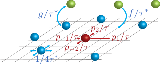
We consider a d𝑑d-dimensional hypercubic lattice (we denote by σ𝜎\sigma its spacing) in contact with a reservoir of particles (see Fig. 1). We adopt a continuous-time description of the system. We assume that the particles in the reservoir adsorb onto empty lattice sites at a fixed rate f/τ𝑓superscript𝜏f/\tau^{*}. The particles adsorbed on the lattice desorb back to the reservoir with a rate g/τ𝑔superscript𝜏g/\tau^{*}. The adsorbed particles perform symmetric nearest-neighbor random walks, and jump to any of the 2d2𝑑2d neighboring sites with a rate 1/(2dτ)12𝑑superscript𝜏1/(2d\tau^{*}). All the particles present on the lattice interact with a hardcore exclusion rule, such that each lattice site is occupied by at most one particle.

We introduce the occupation variable η𝒓subscript𝜂𝒓\eta_{{\boldsymbol{r}}}, which takes two values: 111, if the site 𝒓𝒓{\boldsymbol{r}} is occupied by an adsorbed particle, and 00, otherwise. The mean density of the bath particles, η𝒓delimited-⟨⟩subscript𝜂𝒓\langle\eta_{\boldsymbol{r}}\rangle, is equal to ρ=f/(f+g)𝜌𝑓𝑓𝑔\rho=f/(f+g) in the long-time limit. However, the number of bath particles adsorbed on the lattice is not constant. The case where the number of particles on the lattice is conserved can be retrieved by taking the limits f0𝑓0f\to 0 and g0𝑔0g\to 0 with a fixed value of the density ρ=f/(f+g)𝜌𝑓𝑓𝑔\rho=f/(f+g) .

Refer to caption
Figure 1: Model and notations in the two-dimensional case.

We also introduce a tracer particle (TP). The TP cannot desorb from the lattice and it is submitted to an external force, such that it preferentially jumps in the direction of the unit vector 𝒆1subscript𝒆1\boldsymbol{e}_{1}. We suppose that the TP, whose position at time t𝑡t is a random variable denoted by 𝑿tsubscript𝑿𝑡\boldsymbol{X}_{t}, waits a random time distributed accordingly to an exponential distribution of mean τ𝜏\tau, and attempts to jump onto one of the neighboring sites 𝑿t+𝒆μsubscript𝑿𝑡subscript𝒆𝜇\boldsymbol{X}_{t}+\boldsymbol{e}_{\mu} (𝒆μ{𝒆±1,,𝒆±d}subscript𝒆𝜇subscript𝒆plus-or-minus1subscript𝒆plus-or-minus𝑑\boldsymbol{e}_{\mu}\in\{\boldsymbol{e}_{\pm 1},\cdots,\boldsymbol{e}_{\pm d}\}). For simplicity, we use the notation 𝒆ν𝒆νsubscript𝒆𝜈subscript𝒆𝜈\boldsymbol{e}_{-\nu}\equiv-\boldsymbol{e}_{\nu}. The probability for the TP to jump in direction ν𝜈\nu is denoted by pνsubscript𝑝𝜈p_{\nu}. The equations presented below and their solutions are valid for any choice of the jump probabilities. However, it can be convenient to assume that the bias originates from an external force 𝑭=F𝒆1𝑭𝐹subscript𝒆1\boldsymbol{F}=F\boldsymbol{e}_{1}, so that the jump probability in direction ν𝜈\nu writes

pν=e12β𝑭𝒆νμ{±1,±d}e12β𝑭𝒆μsubscript𝑝𝜈superscripte12𝛽𝑭subscript𝒆𝜈subscript𝜇plus-or-minus1plus-or-minus𝑑superscripte12𝛽𝑭subscript𝒆𝜇p_{\nu}=\frac{\mathrm{e}^{\frac{1}{2}\beta\boldsymbol{F}\cdot{\boldsymbol{e}}_{\nu}}}{\sum_{\mu\in\{\pm 1,...\pm d\}}\mathrm{e}^{\frac{1}{2}\beta\boldsymbol{F}\cdot\boldsymbol{e}_{\mu}}} (3)

where β=1/(kBT)𝛽1subscript𝑘B𝑇\beta=1/(k_{\mathrm{B}}T) is the inverse temperature, and will be taken equal to one. Note that this choice of pνsubscript𝑝𝜈p_{\nu} fulfills the detailed balance condition. After the direction of the jump has been chosen, the TP hops to the target site if it is vacant; it remains on the same site otherwise.

2.2 Master equation

We begin by introducing some auxiliary definitions. We define η{η𝒓}𝜂subscript𝜂𝒓\eta\equiv\{\eta_{\boldsymbol{r}}\} as the entire set of the occupation variables, which is the configuration of the lattice at a given time. Next, we define the joint probability P(𝑿,η;t)𝑃𝑿𝜂𝑡P(\boldsymbol{X},\eta;t), which is the probability for the TP to be at site 𝑿𝑿\boldsymbol{X} at time t𝑡t with the bath particles in a given configuration η𝜂\eta. Next, we define η𝒓,νsuperscript𝜂𝒓𝜈\eta^{{\boldsymbol{r}},\nu} as the configuration obtained from η𝜂\eta by exchanging the occupation numbers of sites 𝒓𝒓{\boldsymbol{r}} and 𝒓+𝒆ν𝒓subscript𝒆𝜈\boldsymbol{r}+\boldsymbol{e}_{\nu} (Kawasaki-type exchange [34] due to the hop of a bath particle) and η^𝒓superscript^𝜂𝒓{\hat{\eta}}^{\boldsymbol{r}} as the configuration obtained from η𝜂\eta by the change η𝒓1η𝒓subscript𝜂𝒓1subscript𝜂𝒓\eta_{\boldsymbol{r}}\to 1-\eta_{\boldsymbol{r}} (Glauber-type exchange [35] due to adsorption/desorption events). The time evolution of the joint probability P(𝑿,η;t)𝑃𝑿𝜂𝑡P(\boldsymbol{X},\eta;t) is given by the master equation :

2dτtP(𝑿,η;t)=2𝑑superscript𝜏subscript𝑡𝑃𝑿𝜂𝑡absent\displaystyle 2d\tau^{*}\partial_{t}P(\boldsymbol{X},\eta;t)= μ=1d𝒓𝑿𝒆μ,𝑿[P(𝑿,η𝒓,μ;t)P(𝑿,η;t)]superscriptsubscript𝜇1𝑑subscript𝒓𝑿subscript𝒆𝜇𝑿delimited-[]𝑃𝑿superscript𝜂𝒓𝜇𝑡𝑃𝑿𝜂𝑡\displaystyle\sum_{\mu=1}^{d}\sum_{{\boldsymbol{r}}\neq\boldsymbol{X}-\boldsymbol{e}_{\mu},\boldsymbol{X}}\left[P(\boldsymbol{X},\eta^{{\boldsymbol{r}},\mu};t)-P(\boldsymbol{X},\eta;t)\right] (4)
+2dττμpμ[(1η𝑿)P(𝑿𝒆μ,η;t)(1η𝑿+𝒆μ)P(𝑿,η;t)]2𝑑superscript𝜏𝜏subscript𝜇subscript𝑝𝜇delimited-[]1subscript𝜂𝑿𝑃𝑿subscript𝒆𝜇𝜂𝑡1subscript𝜂𝑿subscript𝒆𝜇𝑃𝑿𝜂𝑡\displaystyle+\frac{2d\tau^{*}}{\tau}\sum_{\mu}p_{\mu}\left[\left(1-\eta_{\boldsymbol{X}}\right)P(\boldsymbol{X}-\boldsymbol{e}_{\mu},\eta;t)-\left(1-\eta_{\boldsymbol{X}+\boldsymbol{e}_{\mu}}\right)P(\boldsymbol{X},\eta;t)\right]
+2dg𝒓𝑿[(1η𝒓)P(𝑿,η^𝒓;t)η𝒓P(𝑿,η;t)]2𝑑𝑔subscript𝒓𝑿delimited-[]1subscript𝜂𝒓𝑃𝑿superscript^𝜂𝒓𝑡subscript𝜂𝒓𝑃𝑿𝜂𝑡\displaystyle+2dg\sum_{{\boldsymbol{r}}\neq\boldsymbol{X}}\left[\left(1-\eta_{\boldsymbol{r}}\right)P(\boldsymbol{X},\hat{\eta}^{{\boldsymbol{r}}};t)-\eta_{\boldsymbol{r}}P(\boldsymbol{X},\eta;t)\right]
+2df𝒓𝑿[η𝒓P(𝑿,η^𝒓;t)(1η𝒓)P(𝑿,η;t)].2𝑑𝑓subscript𝒓𝑿delimited-[]subscript𝜂𝒓𝑃𝑿superscript^𝜂𝒓𝑡1subscript𝜂𝒓𝑃𝑿𝜂𝑡\displaystyle+2df\sum_{{\boldsymbol{r}}\neq\boldsymbol{X}}\left[\eta_{\boldsymbol{r}}P(\boldsymbol{X},\hat{\eta}^{{\boldsymbol{r}}};t)-\left(1-\eta_{\boldsymbol{r}}\right)P(\boldsymbol{X},\eta;t)\right].

The first term of the right-hand-side of (4) describes the diffusion of adsorbed particles, the second term corresponds to the diffusion of the TP, and the third and fourth terms are associated to the desorption and adsorption events of the bath particles.

If no otherwise specified, the sum over an index μ𝜇\mu runs over the 2d2𝑑2d elements {±1,,±d}plus-or-minus1plus-or-minus𝑑\{\pm 1,\cdots,\pm d\}. In what follows, the brackets delimited-⟨⟩\left\langle\cdot\right\rangle denote an average over the TP position and bath particles configurations with weight P(𝑿,η;t)𝑃𝑿𝜂𝑡P(\boldsymbol{X},\eta;t), and Xt=𝑿t𝒆1subscript𝑋𝑡subscript𝑿𝑡subscript𝒆1X_{t}=\boldsymbol{X}_{t}\cdot\boldsymbol{e}_{1} denotes the position of the TP along the direction of the external force.

3 Equations satisfied by the first cumulants

3.1 Mean position

The time evolution of the first moment Xtdelimited-⟨⟩subscript𝑋𝑡\langle X_{t}\rangle of the TP position can be obtained by multiplying both sides of (4) by (𝑿𝒆1)𝑿subscript𝒆1(\boldsymbol{X}\cdot\boldsymbol{e}_{1}) and summing over all possible configurations (𝑿,η)𝑿𝜂(\boldsymbol{X},\eta). An alternative way to compute Xtdelimited-⟨⟩subscript𝑋𝑡\left\langle X_{t}\right\rangle is to write that during an infinitesimal time interval ΔtΔ𝑡\Delta t, the TP position Xtsubscript𝑋𝑡X_{t} evolves according to

Xt+Δt={Xt+σwith probability p1(1η𝑿t+𝒆1)Δtτ,Xtσwith probability p1(1η𝑿t+𝒆1)Δtτ,Xtwith probability 1p1(1η𝑿t+𝒆1)Δtτp1(1η𝑿t+𝒆1)Δtτ,subscript𝑋𝑡Δ𝑡casessubscript𝑋𝑡𝜎with probability p1(1η𝑿t+𝒆1)Δtτsubscript𝑋𝑡𝜎with probability p1(1η𝑿t+𝒆1)Δtτsubscript𝑋𝑡with probability 1p1(1η𝑿t+𝒆1)Δtτp1(1η𝑿t+𝒆1)ΔtτX_{t+\Delta t}=\begin{cases}X_{t}+\sigma&\text{with probability $p_{1}(1-\eta_{\boldsymbol{X}_{t}+\boldsymbol{e}_{1}})\frac{\Delta t}{\tau}$},\\ X_{t}-\sigma&\text{with probability $p_{-1}(1-\eta_{\boldsymbol{X}_{t}+\boldsymbol{e}_{-1}})\frac{\Delta t}{\tau}$},\\ X_{t}&\text{with probability $1-p_{1}(1-\eta_{\boldsymbol{X}_{t}+\boldsymbol{e}_{1}})\frac{\Delta t}{\tau}-p_{-1}(1-\eta_{\boldsymbol{X}_{t}+\boldsymbol{e}_{-1}})\frac{\Delta t}{\tau}$},\end{cases} (5)

and take the average of this equation. Both methods result in the following exact equation:

ddtXt=στ{p1[1k𝒆1(t)]p1[1k𝒆1(t)]},dd𝑡delimited-⟨⟩subscript𝑋𝑡𝜎𝜏subscript𝑝1delimited-[]1subscript𝑘subscript𝒆1𝑡subscript𝑝1delimited-[]1subscript𝑘subscript𝒆1𝑡\frac{\mathrm{d}}{\mathrm{d}t}\left\langle X_{t}\right\rangle=\frac{\sigma}{\tau}\left\{p_{1}\left[1-k_{\boldsymbol{e}_{1}}(t)\right]-p_{-1}\left[1-k_{\boldsymbol{e}_{-1}}(t)\right]\right\}, (6)

where k𝒓(t)η𝑿t+𝒓subscript𝑘𝒓𝑡delimited-⟨⟩subscript𝜂subscript𝑿𝑡𝒓k_{\boldsymbol{r}}(t)\equiv\left\langle\eta_{\boldsymbol{X}_{t}+\boldsymbol{r}}\right\rangle is the probability of having at time t𝑡t an adsorbed particle at position 𝒓𝒓\boldsymbol{r}, defined in the frame of reference moving with the TP. In other words, k𝒓(t)subscript𝑘𝒓𝑡k_{\boldsymbol{r}}(t) can be thought of as being the density profile as seen from the moving TP.

Note that the approximation obtained by replacing all the local average densities k𝒓(t)subscript𝑘𝒓𝑡k_{\boldsymbol{r}}(t) by the global density ρ𝜌\rho in Eq. (6) (that we will refer to as the trivial mean-field approximation) yields

ddtXt=στ(p1p1)(1ρ).dd𝑡delimited-⟨⟩subscript𝑋𝑡𝜎𝜏subscript𝑝1subscript𝑝11𝜌\frac{\mathrm{d}}{\mathrm{d}t}\left\langle X_{t}\right\rangle=\frac{\sigma}{\tau}(p_{1}-p_{-1})(1-\rho). (7)

A more accurate determination of the evolution of the mean position of the TP is given by Eq. (6) and relies on the calculation of the quantities k𝒆±1(t)subscript𝑘subscript𝒆plus-or-minus1𝑡k_{\boldsymbol{e}_{\pm 1}}(t), which are the mean density of bath particles at the sites in the vicinity of the TP. This actually requires the computation of the density profile k𝒓(t)subscript𝑘𝒓𝑡k_{\boldsymbol{r}}(t) for arbitrary 𝒓𝒓\boldsymbol{r}. The evolution equations for k𝒓(t)subscript𝑘𝒓𝑡k_{\boldsymbol{r}}(t) may be obtained by multiplying the master equation (4) by η𝑿+𝒓subscript𝜂𝑿𝒓\eta_{\boldsymbol{X}+\boldsymbol{r}} and summing over all the configurations of (𝑿,η)𝑿𝜂(\boldsymbol{X},\eta). We get the following equation :

2dτtk𝒓(t)2𝑑superscript𝜏subscript𝑡subscript𝑘𝒓𝑡\displaystyle 2d\tau^{*}\partial_{t}k_{\boldsymbol{r}}(t) =\displaystyle= μ(μδ𝒓,𝒆μμ)k𝒓(t)2d(f+g)k𝒓(t)+2dfsubscript𝜇subscript𝜇subscript𝛿𝒓subscript𝒆𝜇subscript𝜇subscript𝑘𝒓𝑡2𝑑𝑓𝑔subscript𝑘𝒓𝑡2𝑑𝑓\displaystyle\sum_{\mu}\left(\nabla_{\mu}-\delta_{\boldsymbol{r},\boldsymbol{e}_{\mu}}\nabla_{-\mu}\right)k_{\boldsymbol{r}}(t)-2d(f+g)k_{\boldsymbol{r}}(t)+2df (8)
+2dττνpν(1η𝑿t+𝒆ν)νη𝑿t+𝒓,2𝑑superscript𝜏𝜏subscript𝜈subscript𝑝𝜈delimited-⟨⟩1subscript𝜂subscript𝑿𝑡subscript𝒆𝜈subscript𝜈subscript𝜂subscript𝑿𝑡𝒓\displaystyle+\frac{2d\tau^{*}}{\tau}\sum_{\nu}p_{\nu}\left\langle(1-\eta_{\boldsymbol{X}_{t}+\boldsymbol{e}_{\nu}})\nabla_{\nu}\eta_{\boldsymbol{X}_{t}+\boldsymbol{r}}\right\rangle,

where we define the operator μsubscript𝜇\nabla_{\mu} acting on any space-dependent function f𝑓f:

μf(𝒓)=f(𝒓+𝒆μ)f(𝒓).subscript𝜇𝑓𝒓𝑓𝒓subscript𝒆𝜇𝑓𝒓\nabla_{\mu}f(\boldsymbol{r})=f(\boldsymbol{r}+\boldsymbol{e}_{\mu})-f(\boldsymbol{r}). (9)

Eq. (8) is not closed with respect to the density profiles k𝒓subscript𝑘𝒓k_{\boldsymbol{r}}, but involves the correlation functions η𝑿t+𝒆μη𝑿t+𝒓delimited-⟨⟩subscript𝜂subscript𝑿𝑡subscript𝒆𝜇subscript𝜂subscript𝑿𝑡𝒓\left\langle\eta_{\boldsymbol{X}_{t}+\boldsymbol{e}_{\mu}}\eta_{\boldsymbol{X}_{t}+\boldsymbol{r}}\right\rangle. The evolution equations for these correlation functions can be obtained from the master equation (4), and one can show that they actually involve higher-order correlation functions. Consequently, we face the problem of solving an infinite hierarchy of coupled equations for the correlation functions. We then resort to an approximation, obtained by writing the occupation variables as η𝑹=η𝑹+δη𝑹subscript𝜂𝑹delimited-⟨⟩subscript𝜂𝑹𝛿subscript𝜂𝑹\eta_{\boldsymbol{R}}=\left\langle\eta_{\boldsymbol{R}}\right\rangle+\delta\eta_{\boldsymbol{R}}, and by discarding the terms of order (δη𝑹)2superscript𝛿subscript𝜂𝑹2(\delta\eta_{\boldsymbol{R}})^{2}. We obtain

η𝑿t+𝒓η𝑿t+𝒆μdelimited-⟨⟩subscript𝜂subscript𝑿𝑡𝒓subscript𝜂subscript𝑿𝑡subscript𝒆𝜇\displaystyle\left\langle\eta_{\boldsymbol{X}_{t}+{\boldsymbol{r}}}\eta_{\boldsymbol{X}_{t}+\boldsymbol{e}_{\mu}}\right\rangle =\displaystyle= (η𝑿t+𝒓+δη𝑿t+𝒓)(η𝑿t+𝒆μ+δη𝑿t+𝒆μ)delimited-⟨⟩delimited-⟨⟩subscript𝜂subscript𝑿𝑡𝒓𝛿subscript𝜂subscript𝑿𝑡𝒓delimited-⟨⟩subscript𝜂subscript𝑿𝑡subscript𝒆𝜇𝛿subscript𝜂subscript𝑿𝑡subscript𝒆𝜇\displaystyle\left\langle(\left\langle\eta_{\boldsymbol{X}_{t}+\boldsymbol{r}}\right\rangle+\delta\eta_{\boldsymbol{X}_{t}+\boldsymbol{r}})(\left\langle\eta_{\boldsymbol{X}_{t}+\boldsymbol{e}_{\mu}}\right\rangle+\delta\eta_{\boldsymbol{X}_{t}+\boldsymbol{e}_{\mu}})\right\rangle (10)
similar-to-or-equals\displaystyle\simeq η𝑿t+𝒓η𝑿t+𝒆μdelimited-⟨⟩subscript𝜂subscript𝑿𝑡𝒓delimited-⟨⟩subscript𝜂subscript𝑿𝑡subscript𝒆𝜇\displaystyle\left\langle\eta_{\boldsymbol{X}_{t}+{\boldsymbol{r}}}\right\rangle\left\langle\eta_{\boldsymbol{X}_{t}+\boldsymbol{e}_{\mu}}\right\rangle (11)
similar-to-or-equals\displaystyle\simeq k𝒓(t)k𝒆μ(t),subscript𝑘𝒓𝑡subscript𝑘subscript𝒆𝜇𝑡\displaystyle k_{\boldsymbol{r}}(t)k_{\boldsymbol{e}_{\mu}}(t), (12)

which is valid for 𝒓𝒆μ𝒓subscript𝒆𝜇\boldsymbol{r}\neq\boldsymbol{e}_{\mu}. In the particular case where 𝒓=𝒆μ𝒓subscript𝒆𝜇\boldsymbol{r}=\boldsymbol{e}_{\mu}, recalling that η𝑿t+𝒆μ{0,1}subscript𝜂subscript𝑿𝑡subscript𝒆𝜇01\eta_{\boldsymbol{X}_{t}+\boldsymbol{e}_{\mu}}\in\{0,1\}, we get

(η𝑿t+𝒆μ)2delimited-⟨⟩superscriptsubscript𝜂subscript𝑿𝑡subscript𝒆𝜇2\displaystyle\left\langle({\eta_{\boldsymbol{X}_{t}+\boldsymbol{e}_{\mu}}})^{2}\right\rangle =\displaystyle= η𝑿t+𝒆μdelimited-⟨⟩subscript𝜂subscript𝑿𝑡subscript𝒆𝜇\displaystyle\left\langle{\eta_{\boldsymbol{X}_{t}+\boldsymbol{e}_{\mu}}}\right\rangle (13)
=\displaystyle= k𝒆μ(t).subscript𝑘subscript𝒆𝜇𝑡\displaystyle k_{\boldsymbol{e}_{\mu}}(t). (14)

The approximation (12) then relies on the decoupling of the correlation functions η𝑿t+𝒓η𝑿t+𝒆μdelimited-⟨⟩subscript𝜂subscript𝑿𝑡𝒓subscript𝜂subscript𝑿𝑡subscript𝒆𝜇\left\langle\eta_{\boldsymbol{X}_{t}+{\boldsymbol{r}}}\eta_{\boldsymbol{X}_{t}+\boldsymbol{e}_{\mu}}\right\rangle. It can be seen as a mean-field type approximation, and will be generalized later to study the other cumulants of the TP position. It will be referred to as the decoupling approximation in what follows. This approximation will be shown to be very accurate later on.

Using this approximation in Eq. (8), we obtain

2dτtk𝒓(t)=L~k𝒓(t)+2df,2𝑑superscript𝜏subscript𝑡subscript𝑘𝒓𝑡~𝐿subscript𝑘𝒓𝑡2𝑑𝑓2d\tau^{*}\partial_{t}k_{\boldsymbol{r}}(t)=\widetilde{L}k_{\boldsymbol{r}}(t)+2df, (15)

if 𝒓𝒆ν𝒓subscript𝒆𝜈\boldsymbol{r}\neq\boldsymbol{e}_{\nu}. For the sites 𝒓=𝒆ν𝒓subscript𝒆𝜈{\boldsymbol{r}}=\boldsymbol{e}_{\nu} with ν={±1,±2,,±d}𝜈plus-or-minus1plus-or-minus2plus-or-minus𝑑\nu=\{\pm 1,\pm 2,\ldots,\pm d\} we find

2dτtk𝒆ν(t)=[L~+Aν(t)]k𝒆ν(t)+2df,2𝑑superscript𝜏subscript𝑡subscript𝑘subscript𝒆𝜈𝑡delimited-[]~𝐿subscript𝐴𝜈𝑡subscript𝑘subscript𝒆𝜈𝑡2𝑑𝑓2d\tau^{*}\partial_{t}k_{\boldsymbol{e}_{\nu}}(t)=[\widetilde{L}+A_{\nu}(t)]k_{\boldsymbol{e}_{\nu}}(t)+2df, (16)

where L~~𝐿\widetilde{L} is the operator

L~μAμ(t)μ2d(f+g),~𝐿subscript𝜇subscript𝐴𝜇𝑡subscript𝜇2𝑑𝑓𝑔\widetilde{L}\equiv\sum_{\mu}A_{\mu}(t)\nabla_{\mu}-2d(f+g), (17)

and the coefficients Aμ(t)subscript𝐴𝜇𝑡A_{\mu}(t) are defined by

Aμ(t)1+2dττpμ[1k𝒆μ(t)].subscript𝐴𝜇𝑡12𝑑superscript𝜏𝜏subscript𝑝𝜇delimited-[]1subscript𝑘subscript𝒆𝜇𝑡A_{\mu}(t)\equiv 1+\frac{2d\tau^{*}}{\tau}p_{\mu}[1-k_{\boldsymbol{e}_{\mu}}(t)]. (18)

The occupation number of the origin is taken equal to zero by convention. Note that Eq. (16) represents, from the mathematical point of view, the boundary conditions for the general evolution equation (15), imposed on the sites in the immediate vicinity of the TP. Eqs. (15) and (16) together with Eq. (18) thus constitute a closed system of equations which suffices to compute the density profiles k𝒓(t)subscript𝑘𝒓𝑡k_{\boldsymbol{r}}(t). These equations were first obtained by Bénichou et al., and solved in the case of a one-dimensional lattice [24] and of higher-dimensional lattices [27, 26].

3.2 Fluctuations of the TP position

The time evolution of the second moment Xt2delimited-⟨⟩superscriptsubscript𝑋𝑡2\langle{X_{t}}^{2}\rangle is obtained by multiplying the master equation by (𝑿𝒆1)2superscript𝑿subscript𝒆12(\boldsymbol{X}\cdot\boldsymbol{e}_{1})^{2}, and averaging over the TP position and the bath configuration; or, alternatively, averaging the balance equation (5). The details of this calculation are given in A. We get

ddtXt2dd𝑡delimited-⟨⟩superscriptsubscript𝑋𝑡2absent\displaystyle\frac{\mathrm{d}}{\mathrm{d}t}\langle{X_{t}}^{2}\rangle\equiv ddt(𝑿t𝒆1)2dd𝑡delimited-⟨⟩superscriptsubscript𝑿𝑡subscript𝒆12\displaystyle\frac{\mathrm{d}}{\mathrm{d}t}\left\langle(\boldsymbol{X}_{t}\cdot\boldsymbol{e}_{1})^{2}\right\rangle
=\displaystyle= 2στ{p1[Xtg𝒆1(t)]p1[Xtg𝒆1(t)]}2𝜎𝜏subscript𝑝1delimited-[]delimited-⟨⟩subscript𝑋𝑡subscript𝑔subscript𝒆1𝑡subscript𝑝1delimited-[]delimited-⟨⟩subscript𝑋𝑡subscript𝑔subscript𝒆1𝑡\displaystyle\frac{2\sigma}{\tau}\left\{p_{1}\left[\langle X_{t}\rangle-g_{\boldsymbol{e}_{1}}(t)\right]-p_{-1}\left[\langle X_{t}\rangle-g_{\boldsymbol{e}_{-1}}(t)\right]\right\}
+σ2τ{p1[1k𝒆1(t)]+p1[1k𝒆1(t)]},superscript𝜎2𝜏subscript𝑝1delimited-[]1subscript𝑘subscript𝒆1𝑡subscript𝑝1delimited-[]1subscript𝑘subscript𝒆1𝑡\displaystyle+\frac{\sigma^{2}}{\tau}\left\{p_{1}\left[1-k_{\boldsymbol{e}_{1}}(t)\right]+p_{-1}\left[1-k_{\boldsymbol{e}_{-1}}(t)\right]\right\}, (19)

where g𝒓(t)Xtη𝑿t+𝒓subscript𝑔𝒓𝑡delimited-⟨⟩subscript𝑋𝑡subscript𝜂subscript𝑿𝑡𝒓g_{\boldsymbol{r}}(t)\equiv\left\langle X_{t}\,\eta_{\boldsymbol{X}_{t}+{\boldsymbol{r}}}\right\rangle. Knowing that

ddtXt2=2Xt(ddtXt),dd𝑡superscriptdelimited-⟨⟩subscript𝑋𝑡22delimited-⟨⟩subscript𝑋𝑡dd𝑡delimited-⟨⟩subscript𝑋𝑡\frac{\mathrm{d}}{\mathrm{d}t}\langle{X_{t}}\rangle^{2}=2\langle X_{t}\rangle\left(\frac{\mathrm{d}}{\mathrm{d}t}\langle X_{t}\rangle\right), (20)

and using Eq. (6), we can deduce an expression for the second cumulant of the TP position in the first direction:

ddt(Xt2Xt2)=dd𝑡delimited-⟨⟩superscriptsubscript𝑋𝑡2superscriptdelimited-⟨⟩subscript𝑋𝑡2absent\displaystyle\frac{\mathrm{d}}{\mathrm{d}t}\left(\left\langle{X_{t}}^{2}\right\rangle-\left\langle{X_{t}}\right\rangle^{2}\right)= 2στ[p1g~𝒆1(t)p1g~𝒆1(t)]2𝜎𝜏delimited-[]subscript𝑝1subscript~𝑔subscript𝒆1𝑡subscript𝑝1subscript~𝑔subscript𝒆1𝑡\displaystyle-\frac{2\sigma}{\tau}\left[p_{1}\widetilde{g}_{\boldsymbol{e}_{1}}(t)-p_{-1}\widetilde{g}_{\boldsymbol{e}_{-1}}(t)\right]
+σ2τ{p1[1k𝒆1(t)]+p1[1k𝒆1(t)]},superscript𝜎2𝜏subscript𝑝1delimited-[]1subscript𝑘subscript𝒆1𝑡subscript𝑝1delimited-[]1subscript𝑘subscript𝒆1𝑡\displaystyle+\frac{\sigma^{2}}{\tau}\left\{p_{1}\left[1-k_{\boldsymbol{e}_{1}}(t)\right]+p_{-1}\left[1-k_{\boldsymbol{e}_{-1}}(t)\right]\right\}, (21)

where

g~𝒓(t)δXtδη𝑿t+𝒓,subscript~𝑔𝒓𝑡delimited-⟨⟩𝛿subscript𝑋𝑡𝛿subscript𝜂subscript𝑿𝑡𝒓\widetilde{g}_{\boldsymbol{r}}(t)\equiv\left\langle\delta X_{t}\delta\eta_{\boldsymbol{X}_{t}+{\boldsymbol{r}}}\right\rangle, (22)

with δXtXtXt𝛿subscript𝑋𝑡subscript𝑋𝑡delimited-⟨⟩subscript𝑋𝑡\delta X_{t}\equiv X_{t}-\left\langle X_{t}\right\rangle and δη𝑿t+𝒓=η𝑿t+𝒓η𝑿t+𝒓𝛿subscript𝜂subscript𝑿𝑡𝒓subscript𝜂subscript𝑿𝑡𝒓delimited-⟨⟩subscript𝜂subscript𝑿𝑡𝒓\delta\eta_{\boldsymbol{X}_{t}+{\boldsymbol{r}}}=\eta_{\boldsymbol{X}_{t}+{\boldsymbol{r}}}-\left\langle\eta_{\boldsymbol{X}_{t}+{\boldsymbol{r}}}\right\rangle. It then suffices to determine g~𝒆±1(t)subscript~𝑔subscript𝒆plus-or-minus1𝑡\widetilde{g}_{\boldsymbol{e}_{\pm 1}}(t) to compute the fluctuations of the TP position.

In the trivial mean-field approximation, one has k𝒓=ρsubscript𝑘𝒓𝜌k_{\boldsymbol{r}}=\rho and g~𝒓=0subscript~𝑔𝒓0\widetilde{g}_{\boldsymbol{r}}=0 for any 𝒓𝒓\boldsymbol{r}. Eq. (21) then reduces to

ddt(Xt2Xt2)=σ2τ(p1+p1)(1ρ).dd𝑡delimited-⟨⟩superscriptsubscript𝑋𝑡2superscriptdelimited-⟨⟩subscript𝑋𝑡2superscript𝜎2𝜏subscript𝑝1subscript𝑝11𝜌\frac{\mathrm{d}}{\mathrm{d}t}\left(\left\langle{X_{t}}^{2}\right\rangle-\left\langle{X_{t}}\right\rangle^{2}\right)=\frac{\sigma^{2}}{\tau}(p_{1}+p_{-1})(1-\rho). (23)

Note that Eq. (23) corresponds to the standard result for the fluctuations of the position of a biased random walker, where the time t𝑡t is renormalized by the fraction of unoccupied sites 1ρ1𝜌1-\rho. In the particular case of a one-dimensional lattice where p1+p1=1subscript𝑝1subscript𝑝11p_{1}+p_{-1}=1, the fluctuations of the TP position do not depend on the bias. This is in contrast with the case where the TP has a discrete time evolution [36].

The evolution equations for g~𝒓(t)subscript~𝑔𝒓𝑡\widetilde{g}_{\boldsymbol{r}}(t) are obtained by multiplying the master equation (4) by δXη𝑿+𝒓𝛿𝑋subscript𝜂𝑿𝒓\delta X\eta_{\boldsymbol{X}+\boldsymbol{r}} and summing over all the configurations of (𝑿,η)𝑿𝜂(\boldsymbol{X},\eta). The details of the calculation are given in B. We get the following equation

2dτtg~𝒓(t)=2𝑑superscript𝜏subscript𝑡subscript~𝑔𝒓𝑡absent\displaystyle 2d\tau^{*}\partial_{t}\widetilde{g}_{\boldsymbol{r}}(t)= μ(μδ𝒓,𝒆μμ)g~𝒓(t)2d(f+g)g~𝒓(t)subscript𝜇subscript𝜇subscript𝛿𝒓subscript𝒆𝜇subscript𝜇subscript~𝑔𝒓𝑡2𝑑𝑓𝑔subscript~𝑔𝒓𝑡\displaystyle\sum_{\mu}\left(\nabla_{\mu}-\delta_{{\boldsymbol{r}},{\boldsymbol{e}_{\mu}}}\nabla_{-\mu}\right)\widetilde{g}_{\boldsymbol{r}}(t)-2d(f+g)\widetilde{g}_{\boldsymbol{r}}(t)
+2dττμpμδXt(1η𝑿t+𝒆μ)μη𝑿t+𝒓2𝑑superscript𝜏𝜏subscript𝜇subscript𝑝𝜇delimited-⟨⟩𝛿subscript𝑋𝑡1subscript𝜂subscript𝑿𝑡subscript𝒆𝜇subscript𝜇subscript𝜂subscript𝑿𝑡𝒓\displaystyle+\frac{2d\tau^{*}}{\tau}\sum_{\mu}p_{\mu}\left\langle\delta X_{t}(1-\eta_{\boldsymbol{X}_{t}+\boldsymbol{e}_{\mu}})\nabla_{\mu}\eta_{\boldsymbol{X}_{t}+\boldsymbol{r}}\right\rangle
+2dττσ[p1(1η𝑿t+𝒆1)η𝑿t+𝒓+𝒆1p1(1η𝑿t+𝒆1)η𝑿t+𝒓+𝒆1]2𝑑superscript𝜏𝜏𝜎delimited-[]subscript𝑝1delimited-⟨⟩1subscript𝜂subscript𝑿𝑡subscript𝒆1subscript𝜂subscript𝑿𝑡𝒓subscript𝒆1subscript𝑝1delimited-⟨⟩1subscript𝜂subscript𝑿𝑡subscript𝒆1subscript𝜂subscript𝑿𝑡𝒓subscript𝒆1\displaystyle+\frac{2d\tau^{*}}{\tau}\sigma\left[p_{1}\left\langle(1-\eta_{\boldsymbol{X}_{t}+\boldsymbol{e}_{1}})\eta_{\boldsymbol{X}_{t}+\boldsymbol{r}+\boldsymbol{e}_{1}}\right\rangle-p_{-1}\left\langle(1-\eta_{\boldsymbol{X}_{t}+\boldsymbol{e}_{-1}})\eta_{\boldsymbol{X}_{t}+\boldsymbol{r}+\boldsymbol{e}_{-1}}\right\rangle\right]
2dττσ[p1(1k𝒆1)p1(1k𝒆1)]k𝒓(t).2𝑑superscript𝜏𝜏𝜎delimited-[]subscript𝑝11subscript𝑘subscript𝒆1subscript𝑝11subscript𝑘subscript𝒆1subscript𝑘𝒓𝑡\displaystyle-\frac{2d\tau^{*}}{\tau}\sigma\left[p_{1}(1-k_{\boldsymbol{e}_{1}})-p_{-1}(1-k_{\boldsymbol{e}_{-1}})\right]k_{\boldsymbol{r}}(t). (24)

We then notice that this evolution equation involves higher-order correlation functions, of the form δXtη𝑿t+𝒓η𝑿t+𝒆μdelimited-⟨⟩𝛿subscript𝑋𝑡subscript𝜂subscript𝑿𝑡𝒓subscript𝜂subscript𝑿𝑡subscript𝒆𝜇\left\langle\delta X_{t}\eta_{\boldsymbol{X}_{t}+{\boldsymbol{r}}}\eta_{\boldsymbol{X}_{t}+\boldsymbol{e}_{\mu}}\right\rangle. As previously, their computation would lead to an infinite hierarchy of coupled equations. We then write an extension of the decoupling approximation (12), obtained by writing η𝑹=η𝑹+δη𝑹subscript𝜂𝑹delimited-⟨⟩subscript𝜂𝑹𝛿subscript𝜂𝑹\eta_{\boldsymbol{R}}=\left\langle\eta_{\boldsymbol{R}}\right\rangle+\delta\eta_{\boldsymbol{R}} and discarding the terms of order (δη𝑹)2superscript𝛿subscript𝜂𝑹2(\delta\eta_{\boldsymbol{R}})^{2}. We find

δXtη𝑿t+𝒓η𝑿t+𝒆μdelimited-⟨⟩𝛿subscript𝑋𝑡subscript𝜂subscript𝑿𝑡𝒓subscript𝜂subscript𝑿𝑡subscript𝒆𝜇\displaystyle\left\langle\delta X_{t}\eta_{\boldsymbol{X}_{t}+{\boldsymbol{r}}}\eta_{\boldsymbol{X}_{t}+\boldsymbol{e}_{\mu}}\right\rangle similar-to-or-equals\displaystyle\simeq η𝑿t+𝒓δXtη𝑿t+𝒆μ+δXtη𝑿t+𝒓η𝑿t+𝒆μ,delimited-⟨⟩subscript𝜂subscript𝑿𝑡𝒓delimited-⟨⟩𝛿subscript𝑋𝑡subscript𝜂subscript𝑿𝑡subscript𝒆𝜇delimited-⟨⟩𝛿subscript𝑋𝑡subscript𝜂subscript𝑿𝑡𝒓delimited-⟨⟩subscript𝜂subscript𝑿𝑡subscript𝒆𝜇\displaystyle\left\langle\eta_{\boldsymbol{X}_{t}+{\boldsymbol{r}}}\right\rangle\left\langle\delta X_{t}\eta_{\boldsymbol{X}_{t}+\boldsymbol{e}_{\mu}}\right\rangle+\left\langle\delta X_{t}\eta_{\boldsymbol{X}_{t}+\boldsymbol{r}}\right\rangle\left\langle\eta_{\boldsymbol{X}_{t}+\boldsymbol{e}_{\mu}}\right\rangle, (25)
=\displaystyle= k𝒓(t)g~𝒆μ(t)+k𝒆μ(t)g~𝒓(t),subscript𝑘𝒓𝑡subscript~𝑔subscript𝒆𝜇𝑡subscript𝑘subscript𝒆𝜇𝑡subscript~𝑔𝒓𝑡\displaystyle k_{\boldsymbol{r}}(t)\widetilde{g}_{\boldsymbol{e}_{\mu}}(t)+k_{\boldsymbol{e}_{\mu}}(t)\widetilde{g}_{\boldsymbol{r}}(t), (26)

which is valid for 𝒓𝒆μ𝒓subscript𝒆𝜇\boldsymbol{r}\neq\boldsymbol{e}_{\mu}. For 𝒓=𝒆μ𝒓subscript𝒆𝜇\boldsymbol{r}=\boldsymbol{e}_{\mu}, using the relation (η𝑿t+𝒆μ)2=η𝑿t+𝒆μsuperscriptsubscript𝜂subscript𝑿𝑡subscript𝒆𝜇2subscript𝜂subscript𝑿𝑡subscript𝒆𝜇({\eta_{\boldsymbol{X}_{t}+\boldsymbol{e}_{\mu}}})^{2}=\eta_{\boldsymbol{X}_{t}+\boldsymbol{e}_{\mu}}, we obtain

δXt(η𝑿t+𝒆μ)2=g~𝒆μ.delimited-⟨⟩𝛿subscript𝑋𝑡superscriptsubscript𝜂subscript𝑿𝑡subscript𝒆𝜇2subscript~𝑔subscript𝒆𝜇\left\langle\delta X_{t}({\eta_{\boldsymbol{X}_{t}+{\boldsymbol{e}_{\mu}}}})^{2}\right\rangle=\widetilde{g}_{\boldsymbol{e}_{\mu}}. (27)

If 𝒓{𝒆±1,,𝒆±d}𝒓subscript𝒆plus-or-minus1subscript𝒆plus-or-minus𝑑\boldsymbol{r}\notin\{\boldsymbol{e}_{\pm 1},\dots,\boldsymbol{e}_{\pm d}\}, expandind the term of second line of Eq. (24), we obtain

2dττμpμδXt(1η𝑿t+𝒆μ)μη𝑿t+𝒓2𝑑superscript𝜏𝜏subscript𝜇subscript𝑝𝜇delimited-⟨⟩𝛿subscript𝑋𝑡1subscript𝜂subscript𝑿𝑡subscript𝒆𝜇subscript𝜇subscript𝜂subscript𝑿𝑡𝒓\displaystyle\frac{2d\tau^{*}}{\tau}\sum_{\mu}p_{\mu}\left\langle\delta X_{t}(1-\eta_{\boldsymbol{X}_{t}+\boldsymbol{e}_{\mu}})\nabla_{\mu}\eta_{\boldsymbol{X}_{t}+\boldsymbol{r}}\right\rangle
=2dττμpμ[δXtη𝑿t+𝒓+𝒆μδXtη𝑿t+𝒓δXtη𝑿t+𝒆μη𝑿t+𝒓+𝒆μ+δXtη𝑿t+𝒆μη𝑿t+𝒓],absent2𝑑superscript𝜏𝜏subscript𝜇subscript𝑝𝜇delimited-[]delimited-⟨⟩𝛿subscript𝑋𝑡subscript𝜂subscript𝑿𝑡𝒓subscript𝒆𝜇delimited-⟨⟩𝛿subscript𝑋𝑡subscript𝜂subscript𝑿𝑡𝒓delimited-⟨⟩𝛿subscript𝑋𝑡subscript𝜂subscript𝑿𝑡subscript𝒆𝜇subscript𝜂subscript𝑿𝑡𝒓subscript𝒆𝜇delimited-⟨⟩𝛿subscript𝑋𝑡subscript𝜂subscript𝑿𝑡subscript𝒆𝜇subscript𝜂subscript𝑿𝑡𝒓\displaystyle=\frac{2d\tau^{*}}{\tau}\sum_{\mu}p_{\mu}\left[\left\langle\delta X_{t}\eta_{\boldsymbol{X}_{t}+\boldsymbol{r}+\boldsymbol{e}_{\mu}}\right\rangle-\left\langle\delta X_{t}\eta_{\boldsymbol{X}_{t}+\boldsymbol{r}}\right\rangle-\left\langle\delta X_{t}\eta_{\boldsymbol{X}_{t}+\boldsymbol{e}_{\mu}}\eta_{\boldsymbol{X}_{t}+\boldsymbol{r}+\boldsymbol{e}_{\mu}}\right\rangle+\left\langle\delta X_{t}\eta_{\boldsymbol{X}_{t}+\boldsymbol{e}_{\mu}}\eta_{\boldsymbol{X}_{t}+\boldsymbol{r}}\right\rangle\right],

and using the definitions of g~𝒓subscript~𝑔𝒓\widetilde{g}_{\boldsymbol{r}} (Eq. (22)) as well as the decoupling approximation (Eq. (26)), we obtain

2dττμpμδXt(1η𝑿t+𝒆μ)μη𝑿t+𝒓2𝑑superscript𝜏𝜏subscript𝜇subscript𝑝𝜇delimited-⟨⟩𝛿subscript𝑋𝑡1subscript𝜂subscript𝑿𝑡subscript𝒆𝜇subscript𝜇subscript𝜂subscript𝑿𝑡𝒓\displaystyle\frac{2d\tau^{*}}{\tau}\sum_{\mu}p_{\mu}\left\langle\delta X_{t}(1-\eta_{\boldsymbol{X}_{t}+\boldsymbol{e}_{\mu}})\nabla_{\mu}\eta_{\boldsymbol{X}_{t}+\boldsymbol{r}}\right\rangle (29)
=2dττμpμ[μg~𝒓(t)g~𝒆μ(t)μk𝒓(t)k𝒆μ(t)μg~𝒓(t)].absent2𝑑superscript𝜏𝜏subscript𝜇subscript𝑝𝜇delimited-[]subscript𝜇subscript~𝑔𝒓𝑡subscript~𝑔subscript𝒆𝜇𝑡subscript𝜇subscript𝑘𝒓𝑡subscript𝑘subscript𝒆𝜇𝑡subscript𝜇subscript~𝑔𝒓𝑡\displaystyle=\frac{2d\tau^{*}}{\tau}\sum_{\mu}p_{\mu}\left[\nabla_{\mu}\widetilde{g}_{\boldsymbol{r}}(t)-\widetilde{g}_{\boldsymbol{e}_{\mu}}(t)\nabla_{\mu}k_{\boldsymbol{r}}(t)-k_{\boldsymbol{e}_{\mu}}(t)\nabla_{\mu}\widetilde{g}_{\boldsymbol{r}}(t)\right]. (30)

Then, we gather the first three terms of the r.h.s. of Eq. (24) and obtain

μμg~𝒓(t)2d(f+g)g~𝒓(t)+2dττμpμδXt(1η𝑿t+𝒆μ)μη𝑿t+𝒓subscript𝜇subscript𝜇subscript~𝑔𝒓𝑡2𝑑𝑓𝑔subscript~𝑔𝒓𝑡2𝑑superscript𝜏𝜏subscript𝜇subscript𝑝𝜇delimited-⟨⟩𝛿subscript𝑋𝑡1subscript𝜂subscript𝑿𝑡subscript𝒆𝜇subscript𝜇subscript𝜂subscript𝑿𝑡𝒓\displaystyle\sum_{\mu}\nabla_{\mu}\widetilde{g}_{\boldsymbol{r}}(t)-2d(f+g)\widetilde{g}_{\boldsymbol{r}}(t)+\frac{2d\tau^{*}}{\tau}\sum_{\mu}p_{\mu}\left\langle\delta X_{t}(1-\eta_{\boldsymbol{X}_{t}+\boldsymbol{e}_{\mu}})\nabla_{\mu}\eta_{\boldsymbol{X}_{t}+\boldsymbol{r}}\right\rangle
=μ{1+2dττ[1k𝒆μ(t)]}μg~𝒓(t)2d(f+g)g~𝒓(t)2dττμpμg~𝒆μ(t)μk𝒓(t)absentsubscript𝜇12𝑑superscript𝜏𝜏delimited-[]1subscript𝑘subscript𝒆𝜇𝑡subscript𝜇subscript~𝑔𝒓𝑡2𝑑𝑓𝑔subscript~𝑔𝒓𝑡2𝑑superscript𝜏𝜏subscript𝜇subscript𝑝𝜇subscript~𝑔subscript𝒆𝜇𝑡subscript𝜇subscript𝑘𝒓𝑡\displaystyle=\sum_{\mu}\left\{1+\frac{2d\tau^{*}}{\tau}\left[1-k_{\boldsymbol{e}_{\mu}}(t)\right]\right\}\nabla_{\mu}\widetilde{g}_{\boldsymbol{r}}(t)-2d(f+g)\widetilde{g}_{\boldsymbol{r}}(t)-\frac{2d\tau^{*}}{\tau}\sum_{\mu}p_{\mu}\widetilde{g}_{\boldsymbol{e}_{\mu}}(t)\nabla_{\mu}k_{\boldsymbol{r}}(t)
=L~g~𝒓(t)2dττμpμg~𝒆μ(t)μk𝒓(t).absent~𝐿subscript~𝑔𝒓𝑡2𝑑superscript𝜏𝜏subscript𝜇subscript𝑝𝜇subscript~𝑔subscript𝒆𝜇𝑡subscript𝜇subscript𝑘𝒓𝑡\displaystyle=\widetilde{L}\widetilde{g}_{\boldsymbol{r}}(t)-\frac{2d\tau^{*}}{\tau}\sum_{\mu}p_{\mu}\widetilde{g}_{\boldsymbol{e}_{\mu}}(t)\nabla_{\mu}k_{\boldsymbol{r}}(t). (31)

The last two terms of Eq. (24) are recast using the decoupling approximation from Eq. (12). One obtains

2dττσ[p1(1η𝑿t+𝒆1)η𝑿t+𝒓+𝒆1p1(1η𝑿t+𝒆1)η𝑿t+𝒓+𝒆1]2𝑑superscript𝜏𝜏𝜎delimited-[]subscript𝑝1delimited-⟨⟩1subscript𝜂subscript𝑿𝑡subscript𝒆1subscript𝜂subscript𝑿𝑡𝒓subscript𝒆1subscript𝑝1delimited-⟨⟩1subscript𝜂subscript𝑿𝑡subscript𝒆1subscript𝜂subscript𝑿𝑡𝒓subscript𝒆1\displaystyle\frac{2d\tau^{*}}{\tau}\sigma\left[p_{1}\left\langle(1-\eta_{\boldsymbol{X}_{t}+\boldsymbol{e}_{1}})\eta_{\boldsymbol{X}_{t}+\boldsymbol{r}+\boldsymbol{e}_{1}}\right\rangle-p_{-1}\left\langle(1-\eta_{\boldsymbol{X}_{t}+\boldsymbol{e}_{-1}})\eta_{\boldsymbol{X}_{t}+\boldsymbol{r}+\boldsymbol{e}_{-1}}\right\rangle\right]
2dττσ{p1[1k𝒆1(t)]p1[1k𝒆1(t)]}k𝒓(t)2𝑑superscript𝜏𝜏𝜎subscript𝑝1delimited-[]1subscript𝑘subscript𝒆1𝑡subscript𝑝1delimited-[]1subscript𝑘subscript𝒆1𝑡subscript𝑘𝒓𝑡\displaystyle-\frac{2d\tau^{*}}{\tau}\sigma\left\{p_{1}[1-k_{\boldsymbol{e}_{1}}(t)]-p_{-1}[1-k_{\boldsymbol{e}_{-1}}(t)]\right\}k_{\boldsymbol{r}}(t) (32)
=2dττσ[p1(k𝒓+𝒆1k𝒆1k𝒓+𝒆1)p1(k𝒓+𝒆1k𝒆1k𝒓+𝒆1)]absent2𝑑superscript𝜏𝜏𝜎delimited-[]subscript𝑝1subscript𝑘𝒓subscript𝒆1subscript𝑘subscript𝒆1subscript𝑘𝒓subscript𝒆1subscript𝑝1subscript𝑘𝒓subscript𝒆1subscript𝑘subscript𝒆1subscript𝑘𝒓subscript𝒆1\displaystyle=\frac{2d\tau^{*}}{\tau}\sigma\left[p_{1}(k_{\boldsymbol{r}+\boldsymbol{e}_{1}}-k_{\boldsymbol{e}_{1}}k_{\boldsymbol{r}+\boldsymbol{e}_{1}})-p_{-1}(k_{\boldsymbol{r}+\boldsymbol{e}_{-1}}-k_{\boldsymbol{e}_{-1}}k_{\boldsymbol{r}+\boldsymbol{e}_{-1}})\right]
2dττσ{p1[1k𝒆1(t)]p1[1k𝒆1(t)]}k𝒓(t)2𝑑superscript𝜏𝜏𝜎subscript𝑝1delimited-[]1subscript𝑘subscript𝒆1𝑡subscript𝑝1delimited-[]1subscript𝑘subscript𝒆1𝑡subscript𝑘𝒓𝑡\displaystyle-\frac{2d\tau^{*}}{\tau}\sigma\left\{p_{1}[1-k_{\boldsymbol{e}_{1}}(t)]-p_{-1}[1-k_{\boldsymbol{e}_{-1}}(t)]\right\}k_{\boldsymbol{r}}(t) (33)
=2dττσ{p1[1k𝒆1(t)]1k𝒓(t)p1[1k𝒆1(t)]1k𝒓(t)}.absent2𝑑superscript𝜏𝜏𝜎subscript𝑝1delimited-[]1subscript𝑘subscript𝒆1𝑡subscript1subscript𝑘𝒓𝑡subscript𝑝1delimited-[]1subscript𝑘subscript𝒆1𝑡subscript1subscript𝑘𝒓𝑡\displaystyle=\frac{2d\tau^{*}}{\tau}\sigma\left\{p_{1}[1-k_{\boldsymbol{e}_{1}}(t)]\nabla_{1}k_{\boldsymbol{r}}(t)-p_{-1}[1-k_{\boldsymbol{e}_{-1}}(t)]\nabla_{-1}k_{\boldsymbol{r}}(t)\right\}. (34)

Using Eqs. (24), (31) and (34), we finally obtain the following equation for the evolution of the correlation functions g~𝒓subscript~𝑔𝒓\widetilde{g}_{\boldsymbol{r}}:

2dτtg~𝒓(t)=2𝑑superscript𝜏subscript𝑡subscript~𝑔𝒓𝑡absent\displaystyle 2d\tau^{*}\partial_{t}\widetilde{g}_{\boldsymbol{r}}(t)= L~g~𝒓(t)+2dττσ{p1[1k𝒆1(t)]1k𝒓(t)p1[1k𝒆1(t)]1k𝒓(t)}~𝐿subscript~𝑔𝒓𝑡2𝑑superscript𝜏𝜏𝜎subscript𝑝1delimited-[]1subscript𝑘subscript𝒆1𝑡subscript1subscript𝑘𝒓𝑡subscript𝑝1delimited-[]1subscript𝑘subscript𝒆1𝑡subscript1subscript𝑘𝒓𝑡\displaystyle\widetilde{L}\widetilde{g}_{\boldsymbol{r}}(t)+\frac{2d\tau^{*}}{\tau}\sigma\left\{p_{1}[1-k_{\boldsymbol{e}_{1}}(t)]\nabla_{1}k_{\boldsymbol{r}}(t)-p_{-1}[1-k_{\boldsymbol{e}_{-1}}(t)]\nabla_{-1}k_{\boldsymbol{r}}(t)\right\}
2dττμpμg~𝒆μ(t)μk𝒓(t),2𝑑superscript𝜏𝜏subscript𝜇subscript𝑝𝜇subscript~𝑔subscript𝒆𝜇𝑡subscript𝜇subscript𝑘𝒓𝑡\displaystyle-\frac{2d\tau^{*}}{\tau}\sum_{\mu}p_{\mu}\widetilde{g}_{\boldsymbol{e}_{\mu}}(t)\nabla_{\mu}k_{\boldsymbol{r}}(t), (35)

which holds for all 𝒓𝒓\boldsymbol{r}, except for 𝒓={𝟎,𝒆±1,,𝒆±d}𝒓0subscript𝒆plus-or-minus1subscript𝒆plus-or-minus𝑑\boldsymbol{r}=\{{\bf 0},\boldsymbol{e}_{\pm 1},\ldots,\boldsymbol{e}_{\pm d}\}.

On the other hand, for the special sites 𝒓=𝒆ν𝒓subscript𝒆𝜈{\boldsymbol{r}}={\boldsymbol{e}_{\nu}} with ν={±1,,±d}𝜈plus-or-minus1plus-or-minus𝑑\nu=\{\pm 1,\ldots,\pm d\}, the term in the second line of Eq. (24) can be rewritten as

2dττμpμδXt(1η𝑿t+𝒆μ)μη𝑿t+𝒆ν2𝑑superscript𝜏𝜏subscript𝜇subscript𝑝𝜇delimited-⟨⟩𝛿subscript𝑋𝑡1subscript𝜂subscript𝑿𝑡subscript𝒆𝜇subscript𝜇subscript𝜂subscript𝑿𝑡subscript𝒆𝜈\displaystyle\frac{2d\tau^{*}}{\tau}\sum_{\mu}p_{\mu}\left\langle\delta X_{t}(1-\eta_{\boldsymbol{X}_{t}+\boldsymbol{e}_{\mu}})\nabla_{\mu}\eta_{\boldsymbol{X}_{t}+\boldsymbol{e}_{\nu}}\right\rangle (36)
=2dττμpμδXt(1η𝑿t+𝒆μ)(η𝑿t+𝒆ν+𝒆μη𝑿t+𝒆ν)absent2𝑑superscript𝜏𝜏subscript𝜇subscript𝑝𝜇delimited-⟨⟩𝛿subscript𝑋𝑡1subscript𝜂subscript𝑿𝑡subscript𝒆𝜇subscript𝜂subscript𝑿𝑡subscript𝒆𝜈subscript𝒆𝜇subscript𝜂subscript𝑿𝑡subscript𝒆𝜈\displaystyle=\frac{2d\tau^{*}}{\tau}\sum_{\mu}p_{\mu}\left\langle\delta X_{t}(1-\eta_{\boldsymbol{X}_{t}+\boldsymbol{e}_{\mu}})(\eta_{\boldsymbol{X}_{t}+\boldsymbol{e}_{\nu}+\boldsymbol{e}_{\mu}}-\eta_{\boldsymbol{X}_{t}+\boldsymbol{e}_{\nu}})\right\rangle (37)
=2dττμ±νpμδXt(1η𝑿t+𝒆μ)(η𝑿t+𝒆ν+𝒆μη𝑿t+𝒆ν)absent2𝑑superscript𝜏𝜏subscript𝜇plus-or-minus𝜈subscript𝑝𝜇delimited-⟨⟩𝛿subscript𝑋𝑡1subscript𝜂subscript𝑿𝑡subscript𝒆𝜇subscript𝜂subscript𝑿𝑡subscript𝒆𝜈subscript𝒆𝜇subscript𝜂subscript𝑿𝑡subscript𝒆𝜈\displaystyle=\frac{2d\tau^{*}}{\tau}\sum_{\mu\neq\pm\nu}p_{\mu}\left\langle\delta X_{t}(1-\eta_{\boldsymbol{X}_{t}+\boldsymbol{e}_{\mu}})(\eta_{\boldsymbol{X}_{t}+\boldsymbol{e}_{\nu}+\boldsymbol{e}_{\mu}}-\eta_{\boldsymbol{X}_{t}+\boldsymbol{e}_{\nu}})\right\rangle (38)
+2dττpνδXt(1η𝑿t+𝒆ν)(η𝑿t+2𝒆νη𝑿t+𝒆ν)2𝑑superscript𝜏𝜏subscript𝑝𝜈delimited-⟨⟩𝛿subscript𝑋𝑡1subscript𝜂subscript𝑿𝑡subscript𝒆𝜈subscript𝜂subscript𝑿𝑡2subscript𝒆𝜈subscript𝜂subscript𝑿𝑡subscript𝒆𝜈\displaystyle+\frac{2d\tau^{*}}{\tau}p_{\nu}\left\langle\delta X_{t}(1-\eta_{\boldsymbol{X}_{t}+\boldsymbol{e}_{\nu}})(\eta_{\boldsymbol{X}_{t}+2\boldsymbol{e}_{\nu}}-\eta_{\boldsymbol{X}_{t}+\boldsymbol{e}_{\nu}})\right\rangle (39)
+2dττpνδXt(1η𝑿t+𝒆ν)(η𝑿tη𝑿t+𝒆ν).2𝑑superscript𝜏𝜏subscript𝑝𝜈delimited-⟨⟩𝛿subscript𝑋𝑡1subscript𝜂subscript𝑿𝑡subscript𝒆𝜈subscript𝜂subscript𝑿𝑡subscript𝜂subscript𝑿𝑡subscript𝒆𝜈\displaystyle+\frac{2d\tau^{*}}{\tau}p_{-\nu}\left\langle\delta X_{t}(1-\eta_{\boldsymbol{X}_{t}+\boldsymbol{e}_{-\nu}})(\eta_{\boldsymbol{X}_{t}}-\eta_{\boldsymbol{X}_{t}+\boldsymbol{e}_{\nu}})\right\rangle. (40)

The first term can be written in terms of k𝒓subscript𝑘𝒓k_{\boldsymbol{r}} and g~𝒓subscript~𝑔𝒓\widetilde{g}_{\boldsymbol{r}} using Eq. (29). The last two terms are rewritten using the decoupling approximation (Eq. (26)), the property (η𝒓)2=η𝒓superscriptsubscript𝜂𝒓2subscript𝜂𝒓(\eta_{\boldsymbol{r}})^{2}=\eta_{\boldsymbol{r}}, and the conventions k𝟎=g~𝟎=0subscript𝑘0subscript~𝑔00k_{\mathbf{0}}=\widetilde{g}_{\mathbf{0}}=0. We obtain

2dττμpμδXt(1η𝑿t+𝒆μ)μη𝑿t+𝒆ν2𝑑superscript𝜏𝜏subscript𝜇subscript𝑝𝜇delimited-⟨⟩𝛿subscript𝑋𝑡1subscript𝜂subscript𝑿𝑡subscript𝒆𝜇subscript𝜇subscript𝜂subscript𝑿𝑡subscript𝒆𝜈\displaystyle\frac{2d\tau^{*}}{\tau}\sum_{\mu}p_{\mu}\left\langle\delta X_{t}(1-\eta_{\boldsymbol{X}_{t}+\boldsymbol{e}_{\mu}})\nabla_{\mu}\eta_{\boldsymbol{X}_{t}+\boldsymbol{e}_{\nu}}\right\rangle
=\displaystyle= 2dττμ±νpμ[μg~𝒓(t)g~𝒆μ(t)μk𝒓(t)k𝒆μ(t)μg~𝒓(t)]2𝑑superscript𝜏𝜏subscript𝜇plus-or-minus𝜈subscript𝑝𝜇delimited-[]subscript𝜇subscript~𝑔𝒓𝑡subscript~𝑔subscript𝒆𝜇𝑡subscript𝜇subscript𝑘𝒓𝑡subscript𝑘subscript𝒆𝜇𝑡subscript𝜇subscript~𝑔𝒓𝑡\displaystyle\frac{2d\tau^{*}}{\tau}\sum_{\mu\neq\pm\nu}p_{\mu}\left[\nabla_{\mu}\widetilde{g}_{\boldsymbol{r}}(t)-\widetilde{g}_{\boldsymbol{e}_{\mu}}(t)\nabla_{\mu}k_{\boldsymbol{r}}(t)-k_{\boldsymbol{e}_{\mu}}(t)\nabla_{\mu}\widetilde{g}_{\boldsymbol{r}}(t)\right]
+2dττpν{g~2𝒆ν(t)[k𝒆ν(t)g~2𝒆ν(t)+k2𝒆ν(t)g~𝒆ν(t)]}2𝑑superscript𝜏𝜏subscript𝑝𝜈subscript~𝑔2subscript𝒆𝜈𝑡delimited-[]subscript𝑘subscript𝒆𝜈𝑡subscript~𝑔2subscript𝒆𝜈𝑡subscript𝑘2subscript𝒆𝜈𝑡subscript~𝑔subscript𝒆𝜈𝑡\displaystyle+\frac{2d\tau^{*}}{\tau}p_{\nu}\left\{\widetilde{g}_{2\boldsymbol{e}_{\nu}}(t)-[k_{\boldsymbol{e}_{\nu}}(t)\widetilde{g}_{2\boldsymbol{e}_{\nu}}(t)+k_{2\boldsymbol{e}_{\nu}}(t)\widetilde{g}_{\boldsymbol{e}_{\nu}}(t)]\right\}
+2dττpν{g~𝒆ν(t)+[k𝒆ν(t)g~𝒆ν(t)+k𝒆ν(t)g~𝒆ν(t)]}2𝑑superscript𝜏𝜏subscript𝑝𝜈subscript~𝑔subscript𝒆𝜈𝑡delimited-[]subscript𝑘subscript𝒆𝜈𝑡subscript~𝑔subscript𝒆𝜈𝑡subscript𝑘subscript𝒆𝜈𝑡subscript~𝑔subscript𝒆𝜈𝑡\displaystyle+\frac{2d\tau^{*}}{\tau}p_{-\nu}\left\{-\widetilde{g}_{\boldsymbol{e}_{\nu}}(t)+[k_{\boldsymbol{e}_{-\nu}}(t)\widetilde{g}_{\boldsymbol{e}_{\nu}}(t)+k_{\boldsymbol{e}_{\nu}}(t)\widetilde{g}_{\boldsymbol{e}_{-\nu}}(t)]\right\} (41)

Using Eq. (41), and after straightforward computations, the first three terms of the r.h.s. of Eq. (24) yield

μ(μδ𝒆ν,𝒆μμ)g~𝒓(t)2d(f+g)g~𝒆ν(t)+2dττμpμδXt(1η𝑿t+𝒆μ)μη𝑿t+𝒆νsubscript𝜇subscript𝜇subscript𝛿subscript𝒆𝜈subscript𝒆𝜇subscript𝜇subscript~𝑔𝒓𝑡2𝑑𝑓𝑔subscript~𝑔subscript𝒆𝜈𝑡2𝑑superscript𝜏𝜏subscript𝜇subscript𝑝𝜇delimited-⟨⟩𝛿subscript𝑋𝑡1subscript𝜂subscript𝑿𝑡subscript𝒆𝜇subscript𝜇subscript𝜂subscript𝑿𝑡subscript𝒆𝜈\displaystyle\sum_{\mu}\left(\nabla_{\mu}-\delta_{\boldsymbol{e}_{\nu},\boldsymbol{e}_{\mu}}\nabla_{-\mu}\right)\widetilde{g}_{\boldsymbol{r}}(t)-2d(f+g)\widetilde{g}_{\boldsymbol{e}_{\nu}}(t)+\frac{2d\tau^{*}}{\tau}\sum_{\mu}p_{\mu}\left\langle\delta X_{t}(1-\eta_{\boldsymbol{X}_{t}+\boldsymbol{e}_{\mu}})\nabla_{\mu}\eta_{\boldsymbol{X}_{t}+\boldsymbol{e}_{\nu}}\right\rangle
=[L~+Aν(t)]g~𝒆ν(t)2dττpνg~𝒆ν(t)k𝒆ν(t)2dττμpμg~𝒆μ(t)μk𝒆ν(t).absentdelimited-[]~𝐿subscript𝐴𝜈𝑡subscript~𝑔subscript𝒆𝜈𝑡2𝑑superscript𝜏𝜏subscript𝑝𝜈subscript~𝑔subscript𝒆𝜈𝑡subscript𝑘subscript𝒆𝜈𝑡2𝑑superscript𝜏𝜏subscript𝜇subscript𝑝𝜇subscript~𝑔subscript𝒆𝜇𝑡subscript𝜇subscript𝑘subscript𝒆𝜈𝑡\displaystyle=[\widetilde{L}+A_{\nu}(t)]\widetilde{g}_{\boldsymbol{e}_{\nu}}(t)-\frac{2d\tau^{*}}{\tau}p_{\nu}\widetilde{g}_{\boldsymbol{e}_{\nu}}(t)k_{\boldsymbol{e}_{\nu}}(t)-\frac{2d\tau^{*}}{\tau}\sum_{\mu}p_{\mu}\widetilde{g}_{\boldsymbol{e}_{\mu}}(t)\nabla_{\mu}k_{\boldsymbol{e}_{\nu}}(t). (42)

Finally, using again Eq. (34) to rewrite the last two terms of Eq. (24), we obtain the equation verified by g~𝒆ν(t)subscript~𝑔subscript𝒆𝜈𝑡\widetilde{g}_{\boldsymbol{e}_{\nu}}(t) for ν{±1,,±d}𝜈plus-or-minus1plus-or-minus𝑑\nu\in\{\pm 1,\dots,\pm d\}:

2dτtg~𝒆ν(t)=2𝑑superscript𝜏subscript𝑡subscript~𝑔subscript𝒆𝜈𝑡absent\displaystyle 2d\tau^{*}\partial_{t}\widetilde{g}_{\boldsymbol{e}_{\nu}}(t)= [L~+Aν(t)]g~𝒆ν(t)+2dττσ{p1[1k𝒆1(t)]1k𝒆ν(t)p1[1k𝒆1(t)]1k𝒆ν(t)}delimited-[]~𝐿subscript𝐴𝜈𝑡subscript~𝑔subscript𝒆𝜈𝑡2𝑑superscript𝜏𝜏𝜎subscript𝑝1delimited-[]1subscript𝑘subscript𝒆1𝑡subscript1subscript𝑘subscript𝒆𝜈𝑡subscript𝑝1delimited-[]1subscript𝑘subscript𝒆1𝑡subscript1subscript𝑘subscript𝒆𝜈𝑡\displaystyle[\widetilde{L}+A_{\nu}(t)]\widetilde{g}_{\boldsymbol{e}_{\nu}}(t)+\frac{2d\tau^{*}}{\tau}\sigma\left\{p_{1}[1-k_{\boldsymbol{e}_{1}}(t)]\nabla_{1}k_{\boldsymbol{e}_{\nu}}(t)-p_{-1}[1-k_{\boldsymbol{e}_{-1}}(t)]\nabla_{-1}k_{\boldsymbol{e}_{\nu}}(t)\right\}
2dττpνg~𝒆ν(t)k𝒆ν(t)2dττμpμg~𝒆μ(t)μk𝒆ν(t).2𝑑superscript𝜏𝜏subscript𝑝𝜈subscript~𝑔subscript𝒆𝜈𝑡subscript𝑘subscript𝒆𝜈𝑡2𝑑superscript𝜏𝜏subscript𝜇subscript𝑝𝜇subscript~𝑔subscript𝒆𝜇𝑡subscript𝜇subscript𝑘subscript𝒆𝜈𝑡\displaystyle-\frac{2d\tau^{*}}{\tau}p_{\nu}\widetilde{g}_{\boldsymbol{e}_{\nu}}(t)k_{\boldsymbol{e}_{\nu}}(t)-\frac{2d\tau^{*}}{\tau}\sum_{\mu}p_{\mu}\widetilde{g}_{\boldsymbol{e}_{\mu}}(t)\nabla_{\mu}k_{\boldsymbol{e}_{\nu}}(t). (43)

Eqs. (35) and (43) then form a closed system of equations for the quantities g~𝒓(t)subscript~𝑔𝒓𝑡\widetilde{g}_{\boldsymbol{r}}(t), provided that the quantities k𝒆ν(t)subscript𝑘subscript𝒆𝜈𝑡k_{\boldsymbol{e}_{\nu}}(t) are known. Note that Eqs. (35) and (43) are linear in the correlation functions g~𝒓(t)subscript~𝑔𝒓𝑡\widetilde{g}_{\boldsymbol{r}}(t), which can be written explicitly in terms of the density profiles k𝒓(t)subscript𝑘𝒓𝑡k_{\boldsymbol{r}}(t).

The quantities g~𝒆±1(t)subscript~𝑔subscript𝒆plus-or-minus1𝑡\widetilde{g}_{\boldsymbol{e}_{\pm 1}}(t) can be deduced from these equations, and one can compute the evolution of the fluctuations of the TP position using Eq. (21).

3.3 Stationary values

We turn to the limit t𝑡t\to\infty. We assume that the quantities k𝒓(t)subscript𝑘𝒓𝑡k_{\boldsymbol{r}}(t) and g~𝒓(t)subscript~𝑔𝒓𝑡\widetilde{g}_{\boldsymbol{r}}(t) have stationary values, so that

limttk𝒓(t)subscript𝑡subscript𝑡subscript𝑘𝒓𝑡\displaystyle\lim_{t\to\infty}\partial_{t}k_{\boldsymbol{r}}(t) =\displaystyle= 0,0\displaystyle 0, (44)
limttg~𝒓(t)subscript𝑡subscript𝑡subscript~𝑔𝒓𝑡\displaystyle\lim_{t\to\infty}\partial_{t}\widetilde{g}_{\boldsymbol{r}}(t) =\displaystyle= 0.0\displaystyle 0. (45)

The existence of these stationary values will be shown afterwards. We will use the simplified notations:

k𝒓subscript𝑘𝒓\displaystyle k_{\boldsymbol{r}} =\displaystyle= limtk𝒓(t),subscript𝑡subscript𝑘𝒓𝑡\displaystyle\lim_{t\to\infty}k_{\boldsymbol{r}}(t), (46)
g~𝒓subscript~𝑔𝒓\displaystyle\widetilde{g}_{\boldsymbol{r}} =\displaystyle= limtg~𝒓(t),subscript𝑡subscript~𝑔𝒓𝑡\displaystyle\lim_{t\to\infty}\widetilde{g}_{\boldsymbol{r}}(t), (47)
Aμsubscript𝐴𝜇\displaystyle A_{\mu} =\displaystyle= limtAμ(t).subscript𝑡subscript𝐴𝜇𝑡\displaystyle\lim_{t\to\infty}A_{\mu}(t). (48)

We also define the observables:

V𝑉\displaystyle V \displaystyle\equiv limtddtXt,subscript𝑡dd𝑡delimited-⟨⟩subscript𝑋𝑡\displaystyle\lim_{t\to\infty}\frac{\mathrm{d}}{\mathrm{d}t}\left\langle X_{t}\right\rangle, (49)
K𝐾\displaystyle K \displaystyle\equiv limt12ddt(Xt2Xt2)subscript𝑡12dd𝑡delimited-⟨⟩superscriptsubscript𝑋𝑡2superscriptdelimited-⟨⟩subscript𝑋𝑡2\displaystyle\lim_{t\to\infty}\frac{1}{2}\frac{\mathrm{d}}{\mathrm{d}t}\left(\left\langle{X_{t}}^{2}\right\rangle-\left\langle{X_{t}}\right\rangle^{2}\right) (50)

so that V𝑉V and K𝐾K represent respectively the velocity and the diffusion coefficient of the TP in the stationary state. Using Eq. (6), the velocity V𝑉V can be written in terms of the functions k𝒓subscript𝑘𝒓k_{\boldsymbol{r}}:

V=στ[p1(1k𝒆1)p1(1k𝒆1)].𝑉𝜎𝜏delimited-[]subscript𝑝11subscript𝑘subscript𝒆1subscript𝑝11subscript𝑘subscript𝒆1V=\frac{\sigma}{\tau}\left[p_{1}\left(1-k_{\boldsymbol{e}_{1}}\right)-p_{-1}\left(1-k_{\boldsymbol{e}_{-1}}\right)\right]. (51)

Similarly, using Eq. (21), the diffusion coefficient can be written

K=σ22dτ[p1(1k𝒆1)+p1(1k𝒆1)]σdτ(p1g~𝒆1p1g~𝒆1).𝐾superscript𝜎22𝑑𝜏delimited-[]subscript𝑝11subscript𝑘subscript𝒆1subscript𝑝11subscript𝑘subscript𝒆1𝜎𝑑𝜏subscript𝑝1subscript~𝑔subscript𝒆1subscript𝑝1subscript~𝑔subscript𝒆1K=\frac{\sigma^{2}}{2d\tau}\left[p_{1}\left(1-k_{\boldsymbol{e}_{1}}\right)+p_{-1}\left(1-k_{\boldsymbol{e}_{-1}}\right)\right]-\frac{\sigma}{d\tau}\left(p_{1}\widetilde{g}_{\boldsymbol{e}_{1}}-p_{-1}\widetilde{g}_{\boldsymbol{e}_{-1}}\right). (52)

The stationary values of the density profiles k𝒓subscript𝑘𝒓k_{\boldsymbol{r}} (in particular k𝒆±1subscript𝑘subscript𝒆plus-or-minus1k_{\boldsymbol{e}_{\pm 1}} and therefore the velocity V𝑉V) are obtained by solving Eqs. (15) and (16) with tk𝒓(t)=0subscript𝑡subscript𝑘𝒓𝑡0\partial_{t}k_{\boldsymbol{r}}(t)=0. Similarly, solving Eqs. (35) and (43) with tg~𝒓(t)=0subscript𝑡subscript~𝑔𝒓𝑡0\partial_{t}\widetilde{g}_{\boldsymbol{r}}(t)=0, one obtains the stationary values of g~𝒆±1subscript~𝑔subscript𝒆plus-or-minus1\widetilde{g}_{\boldsymbol{e}_{\pm 1}} and the diffusion coefficient K𝐾K.

Note that these stationary equations are valid in any dimension, and allow to compute the velocity and diffusion coefficient of the TP under the approximations presented above (Eqs. (12) and (26)). Their solutions will be presented in the case of a one-dimensional system in section 5.

4 Cumulant generating function

4.1 Governing equations

In the previous sections, using a decoupling approximation, we were able to determine the stationary equations satisfied by the quantities k𝒓=η𝒓subscript𝑘𝒓delimited-⟨⟩subscript𝜂𝒓k_{\boldsymbol{r}}=\left\langle\eta_{\boldsymbol{r}}\right\rangle and g~𝒓=δXtδηXt+𝒓subscript~𝑔𝒓delimited-⟨⟩𝛿subscript𝑋𝑡𝛿subscript𝜂subscript𝑋𝑡𝒓\widetilde{g}_{\boldsymbol{r}}=\left\langle\delta X_{t}\delta\eta_{X_{t}+\boldsymbol{r}}\right\rangle, which are involved in the expression of the stationary velocity V𝑉V (Eq. (51)) and of the stationary diffusion coefficient K𝐾K (Eq. (52)) of the TP. Here, we aim at calculating the higher-order cumulants of Xtsubscript𝑋𝑡X_{t}, defined by

κn(t)1innΨ(u;t)un|u=0,subscript𝜅𝑛𝑡evaluated-at1superscripti𝑛superscript𝑛Ψ𝑢𝑡superscript𝑢𝑛𝑢0\kappa_{n}(t)\equiv\frac{1}{\mathrm{i}^{n}}\left.\frac{\partial^{n}\Psi(u;t)}{\partial u^{n}}\right|_{u=0}, (53)

where the quantity

Ψ(u;t)lneiuXtΨ𝑢𝑡superscriptei𝑢subscript𝑋𝑡\Psi(u;t)\equiv\ln\left\langle\mathrm{e}^{\mathrm{i}uX_{t}}\right\rangle (54)

is known as the second characteristic function (or cumulant generating function) of Xtsubscript𝑋𝑡X_{t}. Using the balance equation (5), we get the relation

eiuXt+Δt=eiu(Xt+σ)Δtτp1(1η𝑿t+𝒆1)+eiu(Xtσ)Δtτp1(1η𝑿t+𝒆1)delimited-⟨⟩superscriptei𝑢subscript𝑋𝑡Δ𝑡delimited-⟨⟩superscriptei𝑢subscript𝑋𝑡𝜎Δ𝑡𝜏subscript𝑝11subscript𝜂subscript𝑿𝑡subscript𝒆1delimited-⟨⟩superscriptei𝑢subscript𝑋𝑡𝜎Δ𝑡𝜏subscript𝑝11subscript𝜂subscript𝑿𝑡subscript𝒆1\displaystyle\left\langle\mathrm{e}^{\mathrm{i}uX_{t+\Delta t}}\right\rangle=\left\langle\mathrm{e}^{\mathrm{i}u(X_{t}+\sigma)}\frac{\Delta t}{\tau}p_{1}(1-\eta_{\boldsymbol{X}_{t}+\boldsymbol{e}_{1}})\right\rangle+\left\langle\mathrm{e}^{\mathrm{i}u(X_{t}-\sigma)}\frac{\Delta t}{\tau}p_{-1}(1-\eta_{\boldsymbol{X}_{t}+\boldsymbol{e}_{-1}})\right\rangle
+eiuXt[1Δtτ(p1(1η𝑿t+𝒆1)+p1(1η𝑿t+𝒆1)].\displaystyle+\left\langle\mathrm{e}^{\mathrm{i}uX_{t}}\left[1-\frac{\Delta t}{\tau}(p_{1}(1-\eta_{\boldsymbol{X}_{t}+\boldsymbol{e}_{1}})+p_{-1}(1-\eta_{\boldsymbol{X}_{t}+\boldsymbol{e}_{-1}})\right]\right\rangle. (55)

Note that this equation involves two different averages: an average over the direction of the step taken by the TP, and an average on the realizations. Eq. (55) leads to

ddteiuXt=p1τ(eiuσ1)eiuXt(1η𝑿t+𝒆1)+p1τ(eiuσ1)eiuXt(1η𝑿t+𝒆1),dd𝑡delimited-⟨⟩superscriptei𝑢subscript𝑋𝑡subscript𝑝1𝜏superscriptei𝑢𝜎1delimited-⟨⟩superscriptei𝑢subscript𝑋𝑡1subscript𝜂subscript𝑿𝑡subscript𝒆1subscript𝑝1𝜏superscriptei𝑢𝜎1delimited-⟨⟩superscriptei𝑢subscript𝑋𝑡1subscript𝜂subscript𝑿𝑡subscript𝒆1\frac{\mathrm{d}}{\mathrm{d}t}\left\langle\mathrm{e}^{\mathrm{i}uX_{t}}\right\rangle=\frac{p_{1}}{\tau}\left(\mathrm{e}^{\mathrm{i}u\sigma}-1\right)\left\langle\mathrm{e}^{\mathrm{i}uX_{t}}(1-\eta_{\boldsymbol{X}_{t}+\boldsymbol{e}_{1}})\right\rangle+\frac{p_{-1}}{\tau}\left(\mathrm{e}^{-\mathrm{i}u\sigma}-1\right)\left\langle\mathrm{e}^{\mathrm{i}uX_{t}}(1-\eta_{\boldsymbol{X}_{t}+\boldsymbol{e}_{-1}})\right\rangle, (56)

and, using the definition of Ψ(u;t)Ψ𝑢𝑡\Psi(u;t) from Eq. (54):

dΨdtdΨd𝑡\displaystyle\frac{\mathrm{d}\Psi}{\mathrm{d}t} =1eiuXtddteiuXtabsent1delimited-⟨⟩superscriptei𝑢subscript𝑋𝑡dd𝑡delimited-⟨⟩superscriptei𝑢subscript𝑋𝑡\displaystyle=\frac{1}{\left\langle\mathrm{e}^{\mathrm{i}uX_{t}}\right\rangle}\frac{\mathrm{d}}{\mathrm{d}t}\left\langle\mathrm{e}^{\mathrm{i}uX_{t}}\right\rangle (57)
=p1τ(eiuσ1)[1eiuXtη𝑿t+𝒆1eiuXt]+p1τ(eiuσ1)[1eiuXtη𝑿t+𝒆1eiuXt].absentsubscript𝑝1𝜏superscriptei𝑢𝜎1delimited-[]1delimited-⟨⟩superscriptei𝑢subscript𝑋𝑡subscript𝜂subscript𝑿𝑡subscript𝒆1delimited-⟨⟩superscriptei𝑢subscript𝑋𝑡subscript𝑝1𝜏superscriptei𝑢𝜎1delimited-[]1delimited-⟨⟩superscriptei𝑢subscript𝑋𝑡subscript𝜂subscript𝑿𝑡subscript𝒆1delimited-⟨⟩superscriptei𝑢subscript𝑋𝑡\displaystyle=\frac{p_{1}}{\tau}\left(\mathrm{e}^{\mathrm{i}u\sigma}-1\right)\left[1-\frac{\left\langle\mathrm{e}^{\mathrm{i}uX_{t}}\eta_{\boldsymbol{X}_{t}+\boldsymbol{e}_{1}}\right\rangle}{\left\langle\mathrm{e}^{\mathrm{i}uX_{t}}\right\rangle}\right]+\frac{p_{-1}}{\tau}\left(\mathrm{e}^{-\mathrm{i}u\sigma}-1\right)\left[1-\frac{\left\langle\mathrm{e}^{\mathrm{i}uX_{t}}\eta_{\boldsymbol{X}_{t}+\boldsymbol{e}_{-1}}\right\rangle}{\left\langle\mathrm{e}^{\mathrm{i}uX_{t}}\right\rangle}\right]. (58)

We define the following correlation functions

w𝒓(u;t)eiuXtη𝑿t+𝒓andw~𝒓(u;t)eiuXtη𝑿t+𝒓eiuXt.subscript𝑤𝒓𝑢𝑡delimited-⟨⟩superscriptei𝑢subscript𝑋𝑡subscript𝜂subscript𝑿𝑡𝒓andsubscript~𝑤𝒓𝑢𝑡delimited-⟨⟩superscriptei𝑢subscript𝑋𝑡subscript𝜂subscript𝑿𝑡𝒓delimited-⟨⟩superscriptei𝑢subscript𝑋𝑡w_{\boldsymbol{r}}(u;t)\equiv\left\langle\mathrm{e}^{\mathrm{i}uX_{t}}\eta_{\boldsymbol{X}_{t}+\boldsymbol{r}}\right\rangle\mathrm{~{}~{}~{}and~{}~{}~{}}\widetilde{w}_{\boldsymbol{r}}(u;t)\equiv\frac{\left\langle\mathrm{e}^{\mathrm{i}uX_{t}}\eta_{\boldsymbol{X}_{t}+\boldsymbol{r}}\right\rangle}{\left\langle\mathrm{e}^{\mathrm{i}uX_{t}}\right\rangle}. (59)

Finally, we obtain the following evolution equation for the cumulant generating function of the TP position:

dΨdt=p1τ(eiuσ1)[1w~𝒆1(u;t)]+p1τ(eiuσ1)[1w~𝒆1(u;t)].dΨd𝑡subscript𝑝1𝜏superscriptei𝑢𝜎1delimited-[]1subscript~𝑤subscript𝒆1𝑢𝑡subscript𝑝1𝜏superscriptei𝑢𝜎1delimited-[]1subscript~𝑤subscript𝒆1𝑢𝑡\frac{\mathrm{d}\Psi}{\mathrm{d}t}=\frac{p_{1}}{\tau}\left(\mathrm{e}^{\mathrm{i}u\sigma}-1\right)\left[1-\widetilde{w}_{\boldsymbol{e}_{1}}(u;t)\right]+\frac{p_{-1}}{\tau}\left(\mathrm{e}^{-\mathrm{i}u\sigma}-1\right)\left[1-\widetilde{w}_{\boldsymbol{e}_{-1}}(u;t)\right]. (60)

Assuming that the quantities w~𝒆1(u;t)subscript~𝑤subscript𝒆1𝑢𝑡\widetilde{w}_{\boldsymbol{e}_{1}}(u;t) and w~𝒆1(u;t)subscript~𝑤subscript𝒆1𝑢𝑡\widetilde{w}_{\boldsymbol{e}_{-1}}(u;t) reach stationary values when t𝑡t\to\infty (their existence will be shown a posteriori), the second characteristic function has the following asymptotic behavior :

Ψ(u;t)tΦ(u)t,Ψ𝑢𝑡𝑡similar-toΦ𝑢𝑡\Psi(u;t)\underset{t\to\infty}{\sim}\Phi(u)t, (61)

with

Φ(u)=p1τ(eiuσ1)[1w~𝒆1(u)]+p1τ(eiuσ1)[1w~𝒆1(u)].Φ𝑢subscript𝑝1𝜏superscriptei𝑢𝜎1delimited-[]1subscript~𝑤subscript𝒆1𝑢subscript𝑝1𝜏superscriptei𝑢𝜎1delimited-[]1subscript~𝑤subscript𝒆1𝑢\Phi(u)=\frac{p_{1}}{\tau}\left(\mathrm{e}^{\mathrm{i}u\sigma}-1\right)\left[1-\widetilde{w}_{\boldsymbol{e}_{1}}(u)\right]+\frac{p_{-1}}{\tau}\left(\mathrm{e}^{-\mathrm{i}u\sigma}-1\right)\left[1-\widetilde{w}_{\boldsymbol{e}_{-1}}(u)\right]. (62)

The relation (61) indicates that all the cumulants of Xtsubscript𝑋𝑡X_{t} are linear in time in the long-time limit. In particular, this implies that the n𝑛n-th moment of the rescaled variable Zt=(XtXt)/Xt2Xt2subscript𝑍𝑡subscript𝑋𝑡delimited-⟨⟩subscript𝑋𝑡delimited-⟨⟩superscriptsubscript𝑋𝑡2superscriptdelimited-⟨⟩subscript𝑋𝑡2Z_{t}=(X_{t}-\left\langle X_{t}\right\rangle)/\sqrt{\left\langle{X_{t}}^{2}\right\rangle-\left\langle X_{t}\right\rangle^{2}} scales as t1n/2superscript𝑡1𝑛2t^{1-n/2} in the long-time limit. All the moments of Ztsubscript𝑍𝑡Z_{t} of order greater than 222 vanish when t𝑡t\to\infty, and Ztsubscript𝑍𝑡Z_{t} is distributed accordingly to a Gaussian distribution at large times.

This calculation allows us to compute the full distribution of Xtsubscript𝑋𝑡X_{t} in the long-time limit. Assuming that the u𝑢u-dependance of w~𝒆±1(u)subscript~𝑤subscript𝒆plus-or-minus1𝑢\widetilde{w}_{\boldsymbol{e}_{\pm 1}}(u) is known, we can derive from the previous equations the probability density function (p.d.f.) Pt(x)Prob[Xt=x]subscript𝑃𝑡𝑥Probdelimited-[]subscript𝑋𝑡𝑥P_{t}(x)\equiv\mathrm{Prob}[X_{t}=x] as follows. The quantity eiuXt=eΨ(u;t)delimited-⟨⟩superscriptei𝑢subscript𝑋𝑡superscripteΨ𝑢𝑡\left\langle\mathrm{e}^{\mathrm{i}uX_{t}}\right\rangle=\mathrm{e}^{\Psi(u;t)} is defined by

eiuXt=x=Pt(x)eiux.delimited-⟨⟩superscriptei𝑢subscript𝑋𝑡superscriptsubscript𝑥subscript𝑃𝑡𝑥superscriptei𝑢𝑥\left\langle\mathrm{e}^{\mathrm{i}uX_{t}}\right\rangle=\sum_{x=-\infty}^{\infty}P_{t}(x)\mathrm{e}^{\mathrm{i}ux}. (63)

eΨ(u;t)superscripteΨ𝑢𝑡\mathrm{e}^{\Psi(u;t)} is then the Fourier transform of the p.d.f. Pt(x)subscript𝑃𝑡𝑥P_{t}(x), which can be obtained by the inverse Fourier transform:

Pt(x)=ππdu2πeiuxeΨ(u;t),subscript𝑃𝑡𝑥superscriptsubscript𝜋𝜋d𝑢2𝜋superscriptei𝑢𝑥superscripteΨ𝑢𝑡P_{t}(x)=\int_{-\pi}^{\pi}\frac{\mathrm{d}u}{2\pi}\mathrm{e}^{-\mathrm{i}ux}\mathrm{e}^{\Psi(u;t)}, (64)

and, using the expression of the long-time limit of Ψ(t)Ψ𝑡\Psi(t) (Eqs. (61) and (62)),

Pt(x)tππdu2πexp{p1tτ(eiuσ1)[1w~𝒆1(u)]+p1tτ(eiuσ1)[1w~𝒆1(u)]iux}.subscript𝑃𝑡𝑥𝑡similar-tosuperscriptsubscript𝜋𝜋d𝑢2𝜋subscript𝑝1𝑡𝜏superscriptei𝑢𝜎1delimited-[]1subscript~𝑤subscript𝒆1𝑢subscript𝑝1𝑡𝜏superscriptei𝑢𝜎1delimited-[]1subscript~𝑤subscript𝒆1𝑢i𝑢𝑥P_{t}(x)\underset{t\to\infty}{\sim}\int_{-\pi}^{\pi}\frac{\mathrm{d}u}{2\pi}\exp\left\{\frac{p_{1}t}{\tau}(\mathrm{e}^{\mathrm{i}u\sigma}-1)[1-\widetilde{w}_{\boldsymbol{e}_{1}}(u)]+\frac{p_{-1}t}{\tau}(\mathrm{e}^{-\mathrm{i}u\sigma}-1)[1-\widetilde{w}_{\boldsymbol{e}_{-1}}(u)]-\mathrm{i}ux\right\}. (65)

Consequently, it suffices to determine the u𝑢u-dependence of w~𝒆±1(u;t)subscript~𝑤subscript𝒆plus-or-minus1𝑢𝑡\widetilde{w}_{\boldsymbol{e}_{\pm 1}}(u;t) to obtain the p.d.f. of the TP position. In what follows, we establish the evolution equations for the quantities w~𝒓(u;t)subscript~𝑤𝒓𝑢𝑡\widetilde{w}_{\boldsymbol{r}}(u;t) starting again from the master equation (4).

4.2 Evolution equations of the quantities w~𝒓(u;t)subscript~𝑤𝒓𝑢𝑡\widetilde{w}_{\boldsymbol{r}}(u;t)

The evolution equation of the correlation functions w𝒓(u;t)subscript𝑤𝒓𝑢𝑡w_{\boldsymbol{r}}(u;t) (defined by Eq. (59)) can be obtained by multiplying both sides of the master equation (4) by the quantity η𝑿+𝒓eiuXsubscript𝜂𝑿𝒓superscriptei𝑢𝑋\eta_{\boldsymbol{X}+\boldsymbol{r}}\mathrm{e}^{\mathrm{i}uX} and averaging with respect to the bath configuration η𝜂\eta and the TP position 𝑿tsubscript𝑿𝑡\boldsymbol{X}_{t}. Extending the method used to derive the evolution equations of the correlation functions g~𝒓(t)subscript~𝑔𝒓𝑡\widetilde{g}_{\boldsymbol{r}}(t) starting from the master equation (4), it is found that w𝒓(u;t)subscript𝑤𝒓𝑢𝑡w_{\boldsymbol{r}}(u;t) obeys the following exact equation (see B):

2dτtw𝒓(u;t)=(μμδ𝒓,𝒆μμ)w𝒓(u;t)2d(f+g)w𝒓(u;t)+2dfeiuXt2𝑑superscript𝜏subscript𝑡subscript𝑤𝒓𝑢𝑡subscript𝜇subscript𝜇subscript𝛿𝒓subscript𝒆𝜇subscript𝜇subscript𝑤𝒓𝑢𝑡2𝑑𝑓𝑔subscript𝑤𝒓𝑢𝑡2𝑑𝑓delimited-⟨⟩superscriptei𝑢subscript𝑋𝑡\displaystyle 2d\tau^{*}\partial_{t}w_{\boldsymbol{r}}(u;t)=\left(\sum_{\mu}\nabla_{\mu}-\delta_{{\boldsymbol{r}},{\boldsymbol{e}_{\mu}}}\nabla_{-\mu}\right)w_{\boldsymbol{r}}(u;t)-2d(f+g)w_{\boldsymbol{r}}(u;t)+2df\left\langle\mathrm{e}^{\mathrm{i}uX_{t}}\right\rangle
+2dττμpμeiuXt(1η𝑿t+𝒆μ)μη𝑿t+𝒓2𝑑superscript𝜏𝜏subscript𝜇subscript𝑝𝜇delimited-⟨⟩superscriptei𝑢subscript𝑋𝑡1subscript𝜂subscript𝑿𝑡subscript𝒆𝜇subscript𝜇subscript𝜂subscript𝑿𝑡𝒓\displaystyle+\frac{2d\tau^{*}}{\tau}\sum_{\mu}p_{\mu}\left\langle\mathrm{e}^{\mathrm{i}uX_{t}}(1-\eta_{\boldsymbol{X}_{t}+\boldsymbol{e}_{\mu}})\nabla_{\mu}\eta_{\boldsymbol{X}_{t}+{\boldsymbol{r}}}\right\rangle
+2dττϵ=±1pϵ(eiuϵσ1)eiuXt(1η𝑿t+𝒆ϵ)η𝑿t+𝒓+𝒆ϵ.2𝑑superscript𝜏𝜏subscriptitalic-ϵplus-or-minus1subscript𝑝italic-ϵsuperscriptei𝑢italic-ϵ𝜎1delimited-⟨⟩superscriptei𝑢subscript𝑋𝑡1subscript𝜂subscript𝑿𝑡subscript𝒆italic-ϵsubscript𝜂subscript𝑿𝑡𝒓subscript𝒆italic-ϵ\displaystyle+\frac{2d\tau^{*}}{\tau}\sum_{\epsilon=\pm 1}p_{\epsilon}\left(\mathrm{e}^{\mathrm{i}u\epsilon\sigma}-1\right)\left\langle\mathrm{e}^{\mathrm{i}uX_{t}}(1-\eta_{\boldsymbol{X}_{t}+\boldsymbol{e}_{\epsilon}})\eta_{\boldsymbol{X}_{t}+{\boldsymbol{r}}+\boldsymbol{e}_{\epsilon}}\right\rangle. (66)

We then make the following decoupling hypothesis:

(eiuXteiuXt)η𝑿t+𝒓η𝑿t+𝒆μsimilar-to-or-equalsdelimited-⟨⟩superscriptei𝑢subscript𝑋𝑡delimited-⟨⟩superscriptei𝑢subscript𝑋𝑡subscript𝜂subscript𝑿𝑡𝒓subscript𝜂subscript𝑿𝑡subscript𝒆𝜇absent\displaystyle\left\langle\left(\mathrm{e}^{\mathrm{i}uX_{t}}-\left\langle\mathrm{e}^{\mathrm{i}uX_{t}}\right\rangle\right)\eta_{\boldsymbol{X}_{t}+\boldsymbol{r}}\eta_{\boldsymbol{X}_{t}+\boldsymbol{e}_{\mu}}\right\rangle\simeq (eiuXteiuXt)η𝑿t+𝒓η𝑿t+𝒆μdelimited-⟨⟩superscriptei𝑢subscript𝑋𝑡delimited-⟨⟩superscriptei𝑢subscript𝑋𝑡subscript𝜂subscript𝑿𝑡𝒓delimited-⟨⟩subscript𝜂subscript𝑿𝑡subscript𝒆𝜇\displaystyle\left\langle\left(\mathrm{e}^{\mathrm{i}uX_{t}}-\left\langle\mathrm{e}^{\mathrm{i}uX_{t}}\right\rangle\right)\eta_{\boldsymbol{X}_{t}+\boldsymbol{r}}\right\rangle\left\langle\eta_{\boldsymbol{X}_{t}+\boldsymbol{e}_{\mu}}\right\rangle
+(eiuXteiuXt)η𝑿t+𝒆μη𝑿t+𝒓,delimited-⟨⟩superscriptei𝑢subscript𝑋𝑡delimited-⟨⟩superscriptei𝑢subscript𝑋𝑡subscript𝜂subscript𝑿𝑡subscript𝒆𝜇delimited-⟨⟩subscript𝜂subscript𝑿𝑡𝒓\displaystyle+\left\langle\left(\mathrm{e}^{\mathrm{i}uX_{t}}-\left\langle\mathrm{e}^{\mathrm{i}uX_{t}}\right\rangle\right)\eta_{\boldsymbol{X}_{t}+\boldsymbol{e}_{\mu}}\right\rangle\left\langle\eta_{\boldsymbol{X}_{t}+\boldsymbol{r}}\right\rangle, (67)

which is valid for 𝒓𝒆μ𝒓subscript𝒆𝜇\boldsymbol{r}\neq\boldsymbol{e}_{\mu}. This is equivalent to

eiuXtη𝑿t+𝒓η𝑿t+𝒆μ=w𝒓(u;t)k𝒆μ(t)+k𝒓(t)w𝒆μ(u;t)eiuXtk𝒓(t)k𝒆μ(t).delimited-⟨⟩superscriptei𝑢subscript𝑋𝑡subscript𝜂subscript𝑿𝑡𝒓subscript𝜂subscript𝑿𝑡subscript𝒆𝜇subscript𝑤𝒓𝑢𝑡subscript𝑘subscript𝒆𝜇𝑡subscript𝑘𝒓𝑡subscript𝑤subscript𝒆𝜇𝑢𝑡delimited-⟨⟩superscriptei𝑢subscript𝑋𝑡subscript𝑘𝒓𝑡subscript𝑘subscript𝒆𝜇𝑡\left\langle\mathrm{e}^{\mathrm{i}uX_{t}}\eta_{\boldsymbol{X}_{t}+\boldsymbol{r}}\eta_{\boldsymbol{X}_{t}+\boldsymbol{e}_{\mu}}\right\rangle=w_{\boldsymbol{r}}(u;t)k_{\boldsymbol{e}_{\mu}}(t)+k_{\boldsymbol{r}}(t)w_{\boldsymbol{e}_{\mu}}(u;t)-\left\langle\mathrm{e}^{\mathrm{i}uX_{t}}\right\rangle k_{\boldsymbol{r}}(t)k_{\boldsymbol{e}_{\mu}}(t). (68)

For 𝒓=𝒆μ𝒓subscript𝒆𝜇\boldsymbol{r}=\boldsymbol{e}_{\mu}, one gets

eiuXt(η𝑿t+𝒆μ)2delimited-⟨⟩superscriptei𝑢subscript𝑋𝑡superscriptsubscript𝜂subscript𝑿𝑡subscript𝒆𝜇2\displaystyle\left\langle\mathrm{e}^{\mathrm{i}uX_{t}}(\eta_{\boldsymbol{X}_{t}+\boldsymbol{e}_{\mu}})^{2}\right\rangle =eiuXtη𝑿t+𝒆μabsentdelimited-⟨⟩superscriptei𝑢subscript𝑋𝑡subscript𝜂subscript𝑿𝑡subscript𝒆𝜇\displaystyle=\left\langle\mathrm{e}^{\mathrm{i}uX_{t}}\eta_{\boldsymbol{X}_{t}+\boldsymbol{e}_{\mu}}\right\rangle (69)
=w𝒆μ(u;t).absentsubscript𝑤subscript𝒆𝜇𝑢𝑡\displaystyle=w_{\boldsymbol{e}_{\mu}}(u;t). (70)

This decoupling approximation is an extension of the approximations (12) and (26): it is obtained by writing the occupation variables as η𝑹=η𝑹+δη𝑹subscript𝜂𝑹delimited-⟨⟩subscript𝜂𝑹𝛿subscript𝜂𝑹\eta_{\boldsymbol{R}}=\left\langle\eta_{\boldsymbol{R}}\right\rangle+\delta\eta_{\boldsymbol{R}}, and discarding the terms of order (δη𝑹)2superscript𝛿subscript𝜂𝑹2(\delta\eta_{\boldsymbol{R}})^{2}. Note that expanding Eq. (68) at order 0 and 1 in u𝑢u, we retrieve the decoupling approximations made for the correlation functions η𝑿t+𝒓η𝑿t+𝒆μdelimited-⟨⟩subscript𝜂subscript𝑿𝑡𝒓subscript𝜂subscript𝑿𝑡subscript𝒆𝜇\left\langle\eta_{\boldsymbol{X}_{t}+{\boldsymbol{r}}}\eta_{\boldsymbol{X}_{t}+\boldsymbol{e}_{\mu}}\right\rangle (Eq. (12)) and δXtη𝑿t+𝒓η𝑿t+𝒆μdelimited-⟨⟩𝛿subscript𝑋𝑡subscript𝜂subscript𝑿𝑡𝒓subscript𝜂subscript𝑿𝑡subscript𝒆𝜇\left\langle\delta X_{t}\eta_{\boldsymbol{X}_{t}+{\boldsymbol{r}}}\eta_{\boldsymbol{X}_{t}+\boldsymbol{e}_{\mu}}\right\rangle (Eq. (26)). Using this approximation in Eq. (66), and following a procedure similar to the one used to derive Eqs. (35) and (43) from Eq. (24) we obtain for 𝒓𝒆ν𝒓subscript𝒆𝜈\boldsymbol{r}\neq\boldsymbol{e}_{\nu},

2dτtw𝒓(u;t)=L~w𝒓(u;t)+2dfeiuXt+2dττμpμ[k𝒆μ(t)eiuXtw𝒆μ(u;t)]μk𝒓(t)2𝑑superscript𝜏subscript𝑡subscript𝑤𝒓𝑢𝑡~𝐿subscript𝑤𝒓𝑢𝑡2𝑑𝑓delimited-⟨⟩superscriptei𝑢subscript𝑋𝑡2𝑑superscript𝜏𝜏subscript𝜇subscript𝑝𝜇delimited-[]subscript𝑘subscript𝒆𝜇𝑡delimited-⟨⟩superscriptei𝑢subscript𝑋𝑡subscript𝑤subscript𝒆𝜇𝑢𝑡subscript𝜇subscript𝑘𝒓𝑡\displaystyle 2d\tau^{*}\partial_{t}w_{\boldsymbol{r}}(u;t)=\widetilde{L}w_{\boldsymbol{r}}(u;t)+2df\left\langle\mathrm{e}^{\mathrm{i}uX_{t}}\right\rangle+\frac{2d\tau^{*}}{\tau}\sum_{\mu}p_{\mu}\left[k_{\boldsymbol{e}_{\mu}}(t)\left\langle\mathrm{e}^{\mathrm{i}uX_{t}}\right\rangle-w_{\boldsymbol{e}_{\mu}}(u;t)\right]\nabla_{\mu}k_{\boldsymbol{r}}(t)
+2dττϵ=±1pϵ(eiuϵσ1){w𝒓+𝒆ϵ(u;t)[1k𝒆ϵ(t)]+k𝒓+𝒆ϵ(t)[eiuXtk𝒆ϵ(t)w𝒆ϵ(u;t)]}.2𝑑superscript𝜏𝜏subscriptitalic-ϵplus-or-minus1subscript𝑝italic-ϵsuperscriptei𝑢italic-ϵ𝜎1subscript𝑤𝒓subscript𝒆italic-ϵ𝑢𝑡delimited-[]1subscript𝑘subscript𝒆italic-ϵ𝑡subscript𝑘𝒓subscript𝒆italic-ϵ𝑡delimited-[]delimited-⟨⟩superscriptei𝑢subscript𝑋𝑡subscript𝑘subscript𝒆italic-ϵ𝑡subscript𝑤subscript𝒆italic-ϵ𝑢𝑡\displaystyle+\frac{2d\tau^{*}}{\tau}\sum_{\epsilon=\pm 1}p_{\epsilon}\left(\mathrm{e}^{\mathrm{i}u\epsilon\sigma}-1\right)\left\{w_{\boldsymbol{r}+\boldsymbol{e}_{\epsilon}}(u;t)[1-k_{\boldsymbol{e}_{\epsilon}}(t)]+k_{\boldsymbol{r}+\boldsymbol{e}_{\epsilon}}(t)\left[\left\langle\mathrm{e}^{\mathrm{i}uX_{t}}\right\rangle k_{\boldsymbol{e}_{\epsilon}}(t)-w_{\boldsymbol{e}_{\epsilon}}(u;t)\right]\right\}.
(71)

For 𝒓=𝒆ν𝒓subscript𝒆𝜈\boldsymbol{r}=\boldsymbol{e}_{\nu}, the evolution equation becomes :

2dτtw𝒆ν(u;t)=[L~+Aν(t)]w𝒆ν(u;t)+2dfeiuXt2𝑑superscript𝜏subscript𝑡subscript𝑤subscript𝒆𝜈𝑢𝑡delimited-[]~𝐿subscript𝐴𝜈𝑡subscript𝑤subscript𝒆𝜈𝑢𝑡2𝑑𝑓delimited-⟨⟩superscriptei𝑢subscript𝑋𝑡\displaystyle 2d\tau^{*}\partial_{t}w_{\boldsymbol{e}_{\nu}}(u;t)=[\widetilde{L}+A_{\nu}(t)]w_{\boldsymbol{e}_{\nu}}(u;t)+2df\left\langle\mathrm{e}^{\mathrm{i}uX_{t}}\right\rangle
+2dττμpμ[k𝒆μ(t)eiuXtw𝒆μ(u;t)]μk𝒆ν(t)+2dττpν[k𝒆ν(t)eiuXtw𝒆ν(u;t)]k𝒆ν(t)2𝑑superscript𝜏𝜏subscript𝜇subscript𝑝𝜇delimited-[]subscript𝑘subscript𝒆𝜇𝑡delimited-⟨⟩superscriptei𝑢subscript𝑋𝑡subscript𝑤subscript𝒆𝜇𝑢𝑡subscript𝜇subscript𝑘subscript𝒆𝜈𝑡2𝑑superscript𝜏𝜏subscript𝑝𝜈delimited-[]subscript𝑘subscript𝒆𝜈𝑡delimited-⟨⟩superscriptei𝑢subscript𝑋𝑡subscript𝑤subscript𝒆𝜈𝑢𝑡subscript𝑘subscript𝒆𝜈𝑡\displaystyle+\frac{2d\tau^{*}}{\tau}\sum_{\mu}p_{\mu}\left[k_{\boldsymbol{e}_{\mu}}(t)\left\langle\mathrm{e}^{\mathrm{i}uX_{t}}\right\rangle-w_{\boldsymbol{e}_{\mu}}(u;t)\right]\nabla_{\mu}k_{\boldsymbol{e}_{\nu}}(t)+\frac{2d\tau^{*}}{\tau}p_{\nu}\left[k_{\boldsymbol{e}_{\nu}}(t)\left\langle\mathrm{e}^{\mathrm{i}uX_{t}}\right\rangle-w_{\boldsymbol{e}_{\nu}}(u;t)\right]k_{\boldsymbol{e}_{\nu}}(t)
+2dττϵ=±1pϵ(eiuϵσ1){w𝒆ν+𝒆ϵ(u;t)[1k𝒆ϵ(t)]+k𝒆ν+𝒆ϵ(t)[eiuXtk𝒆ϵ(t)w𝒆ϵ(u;t)]}.2𝑑superscript𝜏𝜏subscriptitalic-ϵplus-or-minus1subscript𝑝italic-ϵsuperscriptei𝑢italic-ϵ𝜎1subscript𝑤subscript𝒆𝜈subscript𝒆italic-ϵ𝑢𝑡delimited-[]1subscript𝑘subscript𝒆italic-ϵ𝑡subscript𝑘subscript𝒆𝜈subscript𝒆italic-ϵ𝑡delimited-[]delimited-⟨⟩superscriptei𝑢subscript𝑋𝑡subscript𝑘subscript𝒆italic-ϵ𝑡subscript𝑤subscript𝒆italic-ϵ𝑢𝑡\displaystyle+\frac{2d\tau^{*}}{\tau}\sum_{\epsilon=\pm 1}p_{\epsilon}\left(\mathrm{e}^{\mathrm{i}u\epsilon\sigma}-1\right)\left\{w_{\boldsymbol{e}_{\nu}+\boldsymbol{e}_{\epsilon}}(u;t)[1-k_{\boldsymbol{e}_{\epsilon}}(t)]+k_{\boldsymbol{e}_{\nu}+\boldsymbol{e}_{\epsilon}}(t)\left[\left\langle\mathrm{e}^{\mathrm{i}uX_{t}}\right\rangle k_{\boldsymbol{e}_{\epsilon}}(t)-w_{\boldsymbol{e}_{\epsilon}}(u;t)\right]\right\}.
(72)

These equations are conveniently written in terms of the variable w~𝒓(u;t)subscript~𝑤𝒓𝑢𝑡\widetilde{w}_{\boldsymbol{r}}(u;t) by noticing that :

w~𝒓t=subscript~𝑤𝒓𝑡absent\displaystyle\frac{\partial\widetilde{w}_{\boldsymbol{r}}}{\partial t}= 1eiuXtw𝒓(u;t)tw𝒓(u;t)eiuXteiuXtt1delimited-⟨⟩superscriptei𝑢subscript𝑋𝑡subscript𝑤𝒓𝑢𝑡𝑡subscript𝑤𝒓𝑢𝑡delimited-⟨⟩superscriptei𝑢subscript𝑋𝑡delimited-⟨⟩superscriptei𝑢subscript𝑋𝑡𝑡\displaystyle\frac{1}{\left\langle\mathrm{e}^{\mathrm{i}uX_{t}}\right\rangle}\frac{\partial{w}_{\boldsymbol{r}}(u;t)}{\partial t}-\frac{{w}_{\boldsymbol{r}}(u;t)}{\left\langle\mathrm{e}^{\mathrm{i}uX_{t}}\right\rangle}\frac{\partial\left\langle\mathrm{e}^{\mathrm{i}uX_{t}}\right\rangle}{\partial t}
=\displaystyle= 1eiuXtw𝒓tw~𝒓(u;t)Ψt1delimited-⟨⟩superscriptei𝑢subscript𝑋𝑡subscript𝑤𝒓𝑡subscript~𝑤𝒓𝑢𝑡Ψ𝑡\displaystyle\frac{1}{\left\langle\mathrm{e}^{\mathrm{i}uX_{t}}\right\rangle}\frac{\partial{w}_{\boldsymbol{r}}}{\partial t}-\widetilde{w}_{\boldsymbol{r}}(u;t)\frac{\partial\Psi}{\partial t}
=\displaystyle= 1eiuXtw𝒓tw~𝒓(u;t){p1τ(eiuσ1)[1w~𝒆1(u;t)]+p1τ(eiuσ1)[1w~𝒆1(u;t)]}.1delimited-⟨⟩superscriptei𝑢subscript𝑋𝑡subscript𝑤𝒓𝑡subscript~𝑤𝒓𝑢𝑡subscript𝑝1𝜏superscriptei𝑢𝜎1delimited-[]1subscript~𝑤subscript𝒆1𝑢𝑡subscript𝑝1𝜏superscriptei𝑢𝜎1delimited-[]1subscript~𝑤subscript𝒆1𝑢𝑡\displaystyle\frac{1}{\left\langle\mathrm{e}^{\mathrm{i}uX_{t}}\right\rangle}\frac{\partial{w}_{\boldsymbol{r}}}{\partial t}-\widetilde{w}_{\boldsymbol{r}}(u;t)\left\{\frac{p_{1}}{\tau}\left(\mathrm{e}^{\mathrm{i}u\sigma}-1\right)\left[1-\widetilde{w}_{\boldsymbol{e}_{1}}(u;t)\right]+\frac{p_{-1}}{\tau}\left(\mathrm{e}^{-\mathrm{i}u\sigma}-1\right)\left[1-\widetilde{w}_{\boldsymbol{e}_{1}}(u;t)\right]\right\}.

Finally, we divide the evolution equations (71) and (72) by eiuXtdelimited-⟨⟩superscriptei𝑢subscript𝑋𝑡\left\langle\mathrm{e}^{\mathrm{i}uX_{t}}\right\rangle and obtain the evolution equations for w~𝒓(u;t)subscript~𝑤𝒓𝑢𝑡\widetilde{w}_{\boldsymbol{r}}(u;t), for 𝒓𝒆ν𝒓subscript𝒆𝜈\boldsymbol{r}\neq\boldsymbol{e}_{\nu} :

2dτtw~𝒓(u;t)=L~w~𝒓(u;t)+2df+2dττμpμ[k𝒆μ(t)w~𝒆μ(u;t)]μk𝒓(t)2𝑑superscript𝜏subscript𝑡subscript~𝑤𝒓𝑢𝑡~𝐿subscript~𝑤𝒓𝑢𝑡2𝑑𝑓2𝑑superscript𝜏𝜏subscript𝜇subscript𝑝𝜇delimited-[]subscript𝑘subscript𝒆𝜇𝑡subscript~𝑤subscript𝒆𝜇𝑢𝑡subscript𝜇subscript𝑘𝒓𝑡\displaystyle 2d\tau^{*}\partial_{t}\widetilde{w}_{\boldsymbol{r}}(u;t)=\widetilde{L}\widetilde{w}_{\boldsymbol{r}}(u;t)+2df+\frac{2d\tau^{*}}{\tau}\sum_{\mu}p_{\mu}\left[k_{\boldsymbol{e}_{\mu}}(t)-\widetilde{w}_{\boldsymbol{e}_{\mu}}(u;t)\right]\nabla_{\mu}k_{\boldsymbol{r}}(t)
+2dττϵ=±1pϵ(eiuϵσ1){ϵw~𝒓(u;t)k𝒆ϵ(t)[w~𝒓+𝒆ϵ(u;t)k𝒓+𝒆ϵ(t)]w~𝒆ϵ(u;t)[k𝒓+𝒆ϵ(t)w~𝒓(u;t)]},2𝑑superscript𝜏𝜏subscriptitalic-ϵplus-or-minus1subscript𝑝italic-ϵsuperscriptei𝑢italic-ϵ𝜎1subscriptitalic-ϵsubscript~𝑤𝒓𝑢𝑡subscript𝑘subscript𝒆italic-ϵ𝑡delimited-[]subscript~𝑤𝒓subscript𝒆italic-ϵ𝑢𝑡subscript𝑘𝒓subscript𝒆italic-ϵ𝑡subscript~𝑤subscript𝒆italic-ϵ𝑢𝑡delimited-[]subscript𝑘𝒓subscript𝒆italic-ϵ𝑡subscript~𝑤𝒓𝑢𝑡\displaystyle+\frac{2d\tau^{*}}{\tau}\sum_{\epsilon=\pm 1}p_{\epsilon}\left(\mathrm{e}^{\mathrm{i}u\epsilon\sigma}-1\right)\left\{\nabla_{\epsilon}\widetilde{w}_{\boldsymbol{r}}(u;t)-k_{\boldsymbol{e}_{\epsilon}}(t)[\widetilde{w}_{\boldsymbol{r}+\boldsymbol{e}_{\epsilon}}(u;t)-k_{\boldsymbol{r}+\boldsymbol{e}_{\epsilon}}(t)]-\widetilde{w}_{\boldsymbol{e}_{\epsilon}}(u;t)[k_{\boldsymbol{r}+\boldsymbol{e}_{\epsilon}}(t)-\widetilde{w}_{\boldsymbol{r}}(u;t)]\right\},
(74)

and for 𝒓=𝒆ν𝒓subscript𝒆𝜈\boldsymbol{r}=\boldsymbol{e}_{\nu} :

2dτtw~𝒆ν(u;t)=[L~+Aν(t)]w~𝒆ν(u;t)+2df2𝑑superscript𝜏subscript𝑡subscript~𝑤subscript𝒆𝜈𝑢𝑡delimited-[]~𝐿subscript𝐴𝜈𝑡subscript~𝑤subscript𝒆𝜈𝑢𝑡2𝑑𝑓\displaystyle 2d\tau^{*}\partial_{t}\widetilde{w}_{\boldsymbol{e}_{\nu}}(u;t)=[\widetilde{L}+A_{\nu}(t)]\widetilde{w}_{\boldsymbol{e}_{\nu}}(u;t)+2df
+2dττμpμ[k𝒆μ(t)w~𝒆μ(u;t)]μk𝒆ν(t)+2dττpν[k𝒆ν(t)w~𝒆ν(u;t)]k𝒆ν(t)2𝑑superscript𝜏𝜏subscript𝜇subscript𝑝𝜇delimited-[]subscript𝑘subscript𝒆𝜇𝑡subscript~𝑤subscript𝒆𝜇𝑢𝑡subscript𝜇subscript𝑘subscript𝒆𝜈𝑡2𝑑superscript𝜏𝜏subscript𝑝𝜈delimited-[]subscript𝑘subscript𝒆𝜈𝑡subscript~𝑤subscript𝒆𝜈𝑢𝑡subscript𝑘subscript𝒆𝜈𝑡\displaystyle+\frac{2d\tau^{*}}{\tau}\sum_{\mu}p_{\mu}\left[k_{\boldsymbol{e}_{\mu}}(t)-\widetilde{w}_{\boldsymbol{e}_{\mu}}(u;t)\right]\nabla_{\mu}k_{\boldsymbol{e}_{\nu}}(t)+\frac{2d\tau^{*}}{\tau}p_{\nu}\left[k_{\boldsymbol{e}_{\nu}}(t)-\widetilde{w}_{\boldsymbol{e}_{\nu}}(u;t)\right]k_{\boldsymbol{e}_{\nu}}(t)
+2dττϵ=±1pϵ(eiuϵσ1){ϵw~𝒆ν(u;t)k𝒆ϵ(t)[w~𝒆ν+𝒆ϵ(u;t)k𝒆ν+𝒆ϵ(t)]w~𝒆ϵ(u;t)[k𝒆ν+𝒆ϵ(t)w~𝒆ν(u;t)]}2𝑑superscript𝜏𝜏subscriptitalic-ϵplus-or-minus1subscript𝑝italic-ϵsuperscriptei𝑢italic-ϵ𝜎1subscriptitalic-ϵsubscript~𝑤subscript𝒆𝜈𝑢𝑡subscript𝑘subscript𝒆italic-ϵ𝑡delimited-[]subscript~𝑤subscript𝒆𝜈subscript𝒆italic-ϵ𝑢𝑡subscript𝑘subscript𝒆𝜈subscript𝒆italic-ϵ𝑡subscript~𝑤subscript𝒆italic-ϵ𝑢𝑡delimited-[]subscript𝑘subscript𝒆𝜈subscript𝒆italic-ϵ𝑡subscript~𝑤subscript𝒆𝜈𝑢𝑡\displaystyle+\frac{2d\tau^{*}}{\tau}\sum_{\epsilon=\pm 1}p_{\epsilon}\left(\mathrm{e}^{\mathrm{i}u\epsilon\sigma}-1\right)\left\{\nabla_{\epsilon}\widetilde{w}_{\boldsymbol{e}_{\nu}}(u;t)-k_{\boldsymbol{e}_{\epsilon}}(t)[\widetilde{w}_{\boldsymbol{e}_{\nu}+\boldsymbol{e}_{\epsilon}}(u;t)-k_{\boldsymbol{e}_{\nu}+\boldsymbol{e}_{\epsilon}}(t)]-\widetilde{w}_{\boldsymbol{e}_{\epsilon}}(u;t)[k_{\boldsymbol{e}_{\nu}+\boldsymbol{e}_{\epsilon}}(t)-\widetilde{w}_{\boldsymbol{e}_{\nu}}(u;t)]\right\}
(75)

These equations can in principle be solved in the stationary limit t𝑡{t\to\infty}, by setting tw~𝒓(u;t)=0subscript𝑡subscript~𝑤𝒓𝑢𝑡0\partial_{t}\widetilde{w}_{\boldsymbol{r}}(u;t)=0 in Eqs. (74) and (75) and obtaining the values of w~𝒓(u)subscript~𝑤𝒓𝑢\widetilde{w}_{\boldsymbol{r}}(u) satisfying these stationary equations. In particular, this allows us to obtain the u𝑢u-dependence of the functions w~𝒆±1(u)subscript~𝑤subscript𝒆plus-or-minus1𝑢\widetilde{w}_{\boldsymbol{e}_{\pm 1}}(u) and to deduce Pt(x)subscript𝑃𝑡𝑥P_{t}(x) from Eq. (65). These equations are valid in any dimension, and their solution gives the cumulant generating function and the probability distribution function of the TP position.

This resolution will be made explicit in the case of a one-dimensional lattice in section 6.5. We also notice that the functions w~𝒓(u;t)subscript~𝑤𝒓𝑢𝑡\widetilde{w}_{\boldsymbol{r}}(u;t) can be expanded in powers of u𝑢u to compute higher-order cumulants. In particular, we give in the next section the evolution equation satisfied by the third cumulant of the position of the TP.

4.3 Third-order cumulant

In this section, we study the third cumulant of the distribution of Xtsubscript𝑋𝑡X_{t}, which characterizes its skewness. We use Eqs. (74) and (75), describing the evolution of w~𝒓(u;t)subscript~𝑤𝒓𝑢𝑡\widetilde{w}_{\boldsymbol{r}}(u;t), to calculate the third order cumulant. We define the coefficient γ𝛾\gamma by the relation :

γlimt16ddt(XtXt)3.𝛾subscript𝑡16dd𝑡delimited-⟨⟩superscriptsubscript𝑋𝑡delimited-⟨⟩subscript𝑋𝑡3\gamma\equiv\lim_{t\to\infty}\frac{1}{6}\frac{\mathrm{d}}{\mathrm{d}t}{\left\langle\left(X_{t}-\left\langle X_{t}\right\rangle\right)^{3}\right\rangle}. (76)

Recalling the definition of Ψ(t)Ψ𝑡\Psi(t) from Eq. (54), we get the following expansion in powers of u𝑢u:

Ψ(t)=u0iuXt+(iu)22(XtXt)2+(iu)36(XtXt)3+Ψ𝑡𝑢0i𝑢delimited-⟨⟩subscript𝑋𝑡superscripti𝑢22delimited-⟨⟩superscriptsubscript𝑋𝑡delimited-⟨⟩subscript𝑋𝑡2superscripti𝑢36delimited-⟨⟩superscriptsubscript𝑋𝑡delimited-⟨⟩subscript𝑋𝑡3\Psi(t)\underset{u\to 0}{=}\mathrm{i}u\left\langle X_{t}\right\rangle+\frac{(\mathrm{i}u)^{2}}{2}\left\langle\left(X_{t}-\left\langle X_{t}\right\rangle\right)^{2}\right\rangle+\frac{(\mathrm{i}u)^{3}}{6}\left\langle\left(X_{t}-\left\langle X_{t}\right\rangle\right)^{3}\right\rangle+\dots (77)

In the long-time limit, and using the definitions of V𝑉V (Eq. (49)), K𝐾K (Eq. (52)) and γ𝛾\gamma (Eq. (76)), one gets

limtdΨdt=iuV+(iu)2K+(iu)3γ+subscript𝑡dΨd𝑡i𝑢𝑉superscripti𝑢2𝐾superscripti𝑢3𝛾\lim_{t\to\infty}\frac{\mathrm{d}\Psi}{\mathrm{d}t}=\mathrm{i}uV+(\mathrm{i}u)^{2}K+(\mathrm{i}u)^{3}\gamma+\dots (78)

We define the correlation function m~𝒓(t)subscript~𝑚𝒓𝑡\widetilde{m}_{\boldsymbol{r}}(t) by the relation

m~𝒓(t)(XtXt)2η𝑿t+𝒓k𝒓(t)[Xt2Xt2],subscript~𝑚𝒓𝑡delimited-⟨⟩superscriptsubscript𝑋𝑡delimited-⟨⟩subscript𝑋𝑡2subscript𝜂subscript𝑿𝑡𝒓subscript𝑘𝒓𝑡delimited-[]delimited-⟨⟩superscriptsubscript𝑋𝑡2superscriptdelimited-⟨⟩subscript𝑋𝑡2\widetilde{m}_{\boldsymbol{r}}(t)\equiv\left\langle(X_{t}-\langle X_{t}\rangle)^{2}\eta_{\boldsymbol{X}_{t}+{\boldsymbol{r}}}\right\rangle-k_{\boldsymbol{r}}(t)\left[\left\langle{X_{t}}^{2}\right\rangle-\left\langle X_{t}\right\rangle^{2}\right], (79)

so that the expansion of w~𝒓(t)subscript~𝑤𝒓𝑡\widetilde{w}_{\boldsymbol{r}}(t) in powers of u𝑢u writes

w~𝒓(t)=k𝒓(t)+iug~𝒓(t)+(iu)22m~𝒓(t)+𝒪(u3),subscript~𝑤𝒓𝑡subscript𝑘𝒓𝑡𝑖𝑢subscript~𝑔𝒓𝑡superscript𝑖𝑢22subscript~𝑚𝒓𝑡𝒪superscript𝑢3\widetilde{w}_{\boldsymbol{r}}(t)=k_{\boldsymbol{r}}(t)+iu\widetilde{g}_{\boldsymbol{r}}(t)+\frac{(iu)^{2}}{2}\widetilde{m}_{\boldsymbol{r}}(t)+\mathcal{O}\left(u^{3}\right), (80)

where we used the definitions of k𝒓(t)=η𝑿t+𝒓subscript𝑘𝒓𝑡delimited-⟨⟩subscript𝜂subscript𝑿𝑡𝒓k_{\boldsymbol{r}}(t)=\left\langle\eta_{\boldsymbol{X}_{t}+\boldsymbol{r}}\right\rangle and g~𝒓(t)=δXtδη𝑿t+𝒓subscript~𝑔𝒓𝑡delimited-⟨⟩𝛿subscript𝑋𝑡𝛿subscript𝜂subscript𝑿𝑡𝒓\widetilde{g}_{\boldsymbol{r}}(t)=\left\langle\delta X_{t}\delta\eta_{\boldsymbol{X}_{t}+{\boldsymbol{r}}}\right\rangle. Expanding both sides of Eq. (60) up to order 3 in u𝑢u in the limit t𝑡t\rightarrow\infty and using Eq. (78), one gets the following expression for γ𝛾\gamma :

γ=p1στ[16σ2(1k𝒆1)12σg~𝒆112m~𝒆1]p1στ[16σ2(1k𝒆1)+12σg~𝒆112m~𝒆1].𝛾subscript𝑝1𝜎𝜏delimited-[]16superscript𝜎21subscript𝑘subscript𝒆112𝜎subscript~𝑔subscript𝒆112subscript~𝑚subscript𝒆1subscript𝑝1𝜎𝜏delimited-[]16superscript𝜎21subscript𝑘subscript𝒆112𝜎subscript~𝑔subscript𝒆112subscript~𝑚subscript𝒆1\gamma=\frac{p_{1}\sigma}{\tau}\left[\frac{1}{6}\sigma^{2}(1-k_{\boldsymbol{e}_{1}})-\frac{1}{2}\sigma\widetilde{g}_{\boldsymbol{e}_{1}}-\frac{1}{2}\widetilde{m}_{\boldsymbol{e}_{1}}\right]-\frac{p_{-1}\sigma}{\tau}\left[\frac{1}{6}\sigma^{2}(1-k_{\boldsymbol{e}_{-1}})+\frac{1}{2}\sigma\widetilde{g}_{\boldsymbol{e}_{-1}}-\frac{1}{2}\widetilde{m}_{\boldsymbol{e}_{-1}}\right]. (81)

According to Eq. (80), the general evolution equations for w~𝒓(u;t)subscript~𝑤𝒓𝑢𝑡\widetilde{w}_{\boldsymbol{r}}(u;t) (Eqs. (74) and (75)) expanded at order 2 in u𝑢u then give the evolution equations of m~𝒓(t)subscript~𝑚𝒓𝑡\widetilde{m}_{\boldsymbol{r}}(t). We get:

  • for 𝒓𝐞𝝂𝒓subscript𝐞𝝂\boldsymbol{r}\neq\mathbf{e_{\boldsymbol{\nu}}} :

    2dτtm~𝒓(t)=L~m~𝒓(t)2dττμpμm~𝒆μ(t)μk𝒓(t)2𝑑superscript𝜏subscript𝑡subscript~𝑚𝒓𝑡~𝐿subscript~𝑚𝒓𝑡2𝑑superscript𝜏𝜏subscript𝜇subscript𝑝𝜇subscript~𝑚subscript𝒆𝜇𝑡subscript𝜇subscript𝑘𝒓𝑡\displaystyle 2d\tau^{*}\partial_{t}\widetilde{m}_{\boldsymbol{r}}(t)=\widetilde{L}\widetilde{m}_{\boldsymbol{r}}(t)-\frac{2d\tau^{*}}{\tau}\sum_{\mu}p_{\mu}\widetilde{m}_{\boldsymbol{e}_{\mu}}(t)\nabla_{\mu}k_{\boldsymbol{r}}(t)
    +2dττϵ=±1pϵσ{2ϵ[(1k𝒆ϵ(t))ϵg~𝒓(t)g~𝒆ϵ(t)ϵk𝒓(t)]+σ(1k𝒆ϵ(t))ϵk𝒓(t)}.2𝑑superscript𝜏𝜏subscriptitalic-ϵplus-or-minus1subscript𝑝italic-ϵ𝜎2italic-ϵdelimited-[]1subscript𝑘subscript𝒆italic-ϵ𝑡subscriptitalic-ϵsubscript~𝑔𝒓𝑡subscript~𝑔subscript𝒆italic-ϵ𝑡subscriptitalic-ϵsubscript𝑘𝒓𝑡𝜎1subscript𝑘subscript𝒆italic-ϵ𝑡subscriptitalic-ϵsubscript𝑘𝒓𝑡\displaystyle+\frac{2d\tau^{*}}{\tau}\sum_{\epsilon=\pm 1}p_{\epsilon}\sigma\left\{2\epsilon\left[(1-k_{\boldsymbol{e}_{\epsilon}}(t))\nabla_{\epsilon}\widetilde{g}_{\boldsymbol{r}}(t)-\widetilde{g}_{\boldsymbol{e}_{\epsilon}}(t)\nabla_{\epsilon}k_{\boldsymbol{r}}(t)\right]+\sigma(1-k_{\boldsymbol{e}_{\epsilon}}(t))\nabla_{\epsilon}k_{\boldsymbol{r}}(t)\right\}.
  • for 𝒓=𝒆ν𝒓subscript𝒆𝜈\boldsymbol{r}=\boldsymbol{e}_{\nu} :

    2dτtm~𝒆ν(t)=[L~+Aν(t)]m~𝒆ν(t)2dττμpμm~𝒆μ(t)μk𝒆ν(t)2dττpνm~𝒆ν(t)k𝒆ν(t)2𝑑superscript𝜏subscript𝑡subscript~𝑚subscript𝒆𝜈𝑡delimited-[]~𝐿subscript𝐴𝜈𝑡subscript~𝑚subscript𝒆𝜈𝑡2𝑑superscript𝜏𝜏subscript𝜇subscript𝑝𝜇subscript~𝑚subscript𝒆𝜇𝑡subscript𝜇subscript𝑘subscript𝒆𝜈𝑡2𝑑superscript𝜏𝜏subscript𝑝𝜈subscript~𝑚subscript𝒆𝜈𝑡subscript𝑘subscript𝒆𝜈𝑡\displaystyle 2d\tau^{*}\partial_{t}\widetilde{m}_{\boldsymbol{e}_{\nu}}(t)=[\widetilde{L}+A_{\nu}(t)]\widetilde{m}_{\boldsymbol{e}_{\nu}}(t)-\frac{2d\tau^{*}}{\tau}\sum_{\mu}p_{\mu}\widetilde{m}_{\boldsymbol{e}_{\mu}}(t)\nabla_{\mu}k_{\boldsymbol{e}_{\nu}}(t)-\frac{2d\tau^{*}}{\tau}p_{\nu}\widetilde{m}_{\boldsymbol{e}_{\nu}}(t)k_{\boldsymbol{e}_{\nu}}(t)
    +2dττϵ=±1pϵσ{2ϵ[(1k𝒆ϵ(t))ϵg~𝒆ν(t)g~𝒆ϵ(t)ϵk𝒆ν(t)]+σ(1k𝒆ϵ(t))ϵk𝒆ν(t)}.2𝑑superscript𝜏𝜏subscriptitalic-ϵplus-or-minus1subscript𝑝italic-ϵ𝜎2italic-ϵdelimited-[]1subscript𝑘subscript𝒆italic-ϵ𝑡subscriptitalic-ϵsubscript~𝑔subscript𝒆𝜈𝑡subscript~𝑔subscript𝒆italic-ϵ𝑡subscriptitalic-ϵsubscript𝑘subscript𝒆𝜈𝑡𝜎1subscript𝑘subscript𝒆italic-ϵ𝑡subscriptitalic-ϵsubscript𝑘subscript𝒆𝜈𝑡\displaystyle+\frac{2d\tau^{*}}{\tau}\sum_{\epsilon=\pm 1}p_{\epsilon}\sigma\left\{2\epsilon\left[(1-k_{\boldsymbol{e}_{\epsilon}}(t))\nabla_{\epsilon}\widetilde{g}_{\boldsymbol{e}_{\nu}}(t)-\widetilde{g}_{\boldsymbol{e}_{\epsilon}}(t)\nabla_{\epsilon}k_{\boldsymbol{e}_{\nu}}(t)\right]+\sigma(1-k_{\boldsymbol{e}_{\epsilon}}(t))\nabla_{\epsilon}k_{\boldsymbol{e}_{\nu}}(t)\right\}.

In the stationary limit, one computes from Eqs. (4.3) and (4.3) the quantities m~𝒆±1subscript~𝑚subscript𝒆plus-or-minus1\widetilde{m}_{\boldsymbol{e}_{\pm 1}} and then the coefficient γ𝛾\gamma from Eq. (81). This will be made explicit in the case of a one-dimensional lattice in section 5.3.

5 First cumulants and distribution of the TP position in one dimension

In this section, we focus on the one-dimensional version of the general model presented in section 2.1. This situation is related to a number of lattice models of interacting particles which have been widely studied in the mathematical and physical literature. In particular, in the situation where the number of particles on the lattice is conserved and where the TP is not biased, the model corresponds to the well-known single file problem, for which several results have been derived exactly [37, 38, 39, 40, 41, 42, 43, 44].

In what follows, we consider the equations derived in the previous section in the particular case of a one-dimensional lattice. We first recall the solutions of the equations satisfied by the density profiles k𝒓subscript𝑘𝒓k_{\boldsymbol{r}} that were obtained in previous studies, and give a detailed resolution of the equations verified by the correlation functions g~𝒓subscript~𝑔𝒓\widetilde{g}_{\boldsymbol{r}} and w~𝒓subscript~𝑤𝒓\widetilde{w}_{\boldsymbol{r}}.

5.1 Solution of the equation on k𝒓subscript𝑘𝒓k_{\boldsymbol{r}} in one dimension

The solutions of the equations verified by k𝒓subscript𝑘𝒓k_{\boldsymbol{r}} have already been presented [24], and we recall them here for completeness. In one dimension, we adopt the simplified notation k𝒓=kn𝒆1knsubscript𝑘𝒓subscript𝑘𝑛subscript𝒆1subscript𝑘𝑛k_{\boldsymbol{r}}=k_{n\boldsymbol{e}_{1}}\equiv k_{n}. The stationary limit of the general equation verified by the density profiles (Eq. (15)) is then a second order recurrence relation on the quantities knsubscript𝑘𝑛k_{n}. Its solution has the following form:

kn={ρ+K+r1nfor n>0,ρ+Kr2nfor n<0,subscript𝑘𝑛cases𝜌subscript𝐾superscriptsubscript𝑟1𝑛for n>0𝜌subscript𝐾superscriptsubscript𝑟2𝑛for n<0k_{n}=\begin{cases}\rho+K_{+}{r_{1}}^{n}&\text{for $n>0$},\\ \rho+K_{-}{r_{2}}^{n}&\text{for $n<0$},\end{cases} (84)

where

r12=A1+A1+2(f+g)(A1+A1+2(f+g))24A1A12A1,subscript𝑟12minus-or-plussubscript𝐴1subscript𝐴12𝑓𝑔superscriptsubscript𝐴1subscript𝐴12𝑓𝑔24subscript𝐴1subscript𝐴12subscript𝐴1r_{\begin{subarray}{c}1\\ 2\end{subarray}}=\frac{A_{1}+A_{-1}+2(f+g)\mp\sqrt{\Big{(}A_{1}+A_{-1}+2(f+g)\Big{)}^{2}-4A_{1}A_{-1}}}{2A_{1}}, (85)

while the amplitudes K±subscript𝐾plus-or-minusK_{\pm} are given respectively by

K+=ρA1A1A1A1r1,subscript𝐾𝜌subscript𝐴1subscript𝐴1subscript𝐴1subscript𝐴1subscript𝑟1K_{+}=\rho\frac{A_{1}-A_{-1}}{A_{-1}-A_{1}r_{1}}, (86)

and

K=ρA1A1A1/r2A1.subscript𝐾𝜌subscript𝐴1subscript𝐴1subscript𝐴1subscript𝑟2subscript𝐴1K_{-}=\rho\frac{A_{1}-A_{-1}}{A_{-1}/r_{2}-A_{1}}. (87)

We notice that r2>r1subscript𝑟2subscript𝑟1r_{2}>r_{1}, which indicates that the density profile behind the TP decreases slower than in front of it. We also note that K+>0subscript𝐾0K_{+}>0 and K<0subscript𝐾0K_{-}<0 which indicates that there is a jammed region ahead of the TP, and, on the contrary, a depleted region behind it.

One obtains a closed sed of two non-linear equations determining implicitly the parameters A1subscript𝐴1A_{1} and A1subscript𝐴1A_{-1}, from which one can compute the TP stationary velocity, related to A±1subscript𝐴plus-or-minus1A_{\pm 1} through

V=σ2τ(A1A1).𝑉𝜎2superscript𝜏subscript𝐴1subscript𝐴1V=\frac{\sigma}{2\tau^{*}}(A_{1}-A_{-1}). (88)

Substituting Eq. (84) into the definition of Aμsubscript𝐴𝜇A_{\mu} (Eq. (18)), we find

A1subscript𝐴1\displaystyle A_{1} =\displaystyle= 1+2p1ττ[1ρρA1A1A1/r1A1],12subscript𝑝1superscript𝜏𝜏delimited-[]1𝜌𝜌subscript𝐴1subscript𝐴1subscript𝐴1subscript𝑟1subscript𝐴1\displaystyle 1+\frac{2p_{1}\tau^{*}}{\tau}\left[1-\rho-\rho\frac{A_{1}-A_{-1}}{A_{-1}/r_{1}-A_{1}}\right], (89)
A1subscript𝐴1\displaystyle A_{-1} =\displaystyle= 1+2p1ττ[1ρρA1A1A1A1r2].12subscript𝑝1superscript𝜏𝜏delimited-[]1𝜌𝜌subscript𝐴1subscript𝐴1subscript𝐴1subscript𝐴1subscript𝑟2\displaystyle 1+\frac{2p_{-1}\tau^{*}}{\tau}\left[1-\rho-\rho\frac{A_{1}-A_{-1}}{A_{-1}-A_{1}r_{2}}\right]. (90)

For a given set of parameters (f𝑓f, g𝑔g, σ𝜎\sigma, τ𝜏\tau, τsuperscript𝜏\tau^{*} and p1subscript𝑝1p_{1}), the numerical resolution of this system leads to the values of A1subscript𝐴1A_{1} and A1subscript𝐴1A_{-1} and then, using Eq. (88), to the value of the stationary velocity of the TP. This approximated value of the stationary velocity will be compared to numerical simulations in section 6.2.

5.2 Solution of the equation on g~𝒓subscript~𝑔𝒓\widetilde{g}_{\boldsymbol{r}} in one dimension

We now go one step further and determine the diffusion coefficient K𝐾K. This in turn requires the knowledge of the functions g~𝒓subscript~𝑔𝒓\widetilde{g}_{\boldsymbol{r}}. For simplicity, we adopt the notations g~𝒓=g~n𝒆1=g~nsubscript~𝑔𝒓subscript~𝑔𝑛subscript𝒆1subscript~𝑔𝑛\widetilde{g}_{\boldsymbol{r}}=\widetilde{g}_{n\boldsymbol{e}_{1}}=\widetilde{g}_{n}. Using the expressions of knsubscript𝑘𝑛k_{n} from Eq. (84), the general equations satisfied by g~nsubscript~𝑔𝑛\widetilde{g}_{n} (Eqs. (35) and (43)) become:

  • for n>1𝑛1n>1:

    A1(g~n+1g~n)+A1(g~n1g~n)2(f+g)g~nsubscript𝐴1subscript~𝑔𝑛1subscript~𝑔𝑛subscript𝐴1subscript~𝑔𝑛1subscript~𝑔𝑛2𝑓𝑔subscript~𝑔𝑛\displaystyle A_{1}(\widetilde{g}_{n+1}-\widetilde{g}_{n})+A_{-1}(\widetilde{g}_{n-1}-\widetilde{g}_{n})-2(f+g)\widetilde{g}_{n} (91)
    +\displaystyle+ 2ττσ{p1K+r1n(1ρK+r1g~1σ)(r11)\displaystyle\frac{2\tau^{*}}{\tau}\sigma\left\{p_{1}K_{+}r_{1}^{n}\left(1-\rho-K_{+}r_{1}-\frac{\widetilde{g}_{1}}{\sigma}\right)(r_{1}-1)\right.
    \displaystyle- p1K+r1n(1ρK+r1+g~1σ)(r111)}=0,\displaystyle\left.p_{-1}K_{+}r_{1}^{n}\left(1-\rho-K_{+}r_{1}+\frac{\widetilde{g}_{-1}}{\sigma}\right)(r_{1}^{-1}-1)\right\}=0,
  • for n<1𝑛1n<-1:

    A1(g~n+1g~n)+A1(g~n1g~n)2(f+g)g~nsubscript𝐴1subscript~𝑔𝑛1subscript~𝑔𝑛subscript𝐴1subscript~𝑔𝑛1subscript~𝑔𝑛2𝑓𝑔subscript~𝑔𝑛\displaystyle A_{1}(\widetilde{g}_{n+1}-\widetilde{g}_{n})+A_{-1}(\widetilde{g}_{n-1}-\widetilde{g}_{n})-2(f+g)\widetilde{g}_{n} (92)
    +\displaystyle+ 2ττσ{p1Kr2n(1ρK+r1g~1σ)(r21)\displaystyle\frac{2\tau^{*}}{\tau}\sigma\left\{p_{1}K_{-}r_{2}^{n}\left(1-\rho-K_{+}r_{1}-\frac{\widetilde{g}_{1}}{\sigma}\right)(r_{2}-1)\right.
    \displaystyle- p1Kr2n(1ρK+r1+g~1σ)(r211)}=0,\displaystyle\left.p_{-1}K_{-}r_{2}^{n}\left(1-\rho-K_{+}r_{1}+\frac{\widetilde{g}_{-1}}{\sigma}\right)(r_{2}^{-1}-1)\right\}=0,
  • g~1subscript~𝑔1\widetilde{g}_{1} and g~1subscript~𝑔1\widetilde{g}_{-1} may be computed using the boundary conditions given by Eq. (43):

    A1g~2g~1(A1+2(f+g)+2ττp1(ρ+K+r12))+2ττp1(ρ+K+r1)g~1subscript𝐴1subscript~𝑔2subscript~𝑔1subscript𝐴12𝑓𝑔2superscript𝜏𝜏subscript𝑝1𝜌subscript𝐾superscriptsubscript𝑟122superscript𝜏𝜏subscript𝑝1𝜌subscript𝐾subscript𝑟1subscript~𝑔1\displaystyle A_{1}\widetilde{g}_{2}-\widetilde{g}_{1}\left(A_{-1}+2(f+g)+\frac{2\tau^{*}}{\tau}p_{1}(\rho+K_{+}r_{1}^{2})\right)+\frac{2\tau^{*}}{\tau}p_{-1}(\rho+K_{+}r_{1})\widetilde{g}_{-1}
    =2ττσp1(1ρK+r1)(ρ+K+r12)absent2superscript𝜏𝜏𝜎subscript𝑝11𝜌subscript𝐾subscript𝑟1𝜌subscript𝐾superscriptsubscript𝑟12\displaystyle=-\frac{2\tau^{*}}{\tau}\sigma p_{1}(1-\rho-K_{+}r_{1})(\rho+K_{+}r_{1}^{2})
    +2ττσ(p1(1ρK+r1)p1(1ρKr21))(ρ+K+r1),2superscript𝜏𝜏𝜎subscript𝑝11𝜌subscript𝐾subscript𝑟1subscript𝑝11𝜌subscript𝐾superscriptsubscript𝑟21𝜌subscript𝐾subscript𝑟1\displaystyle+\frac{2\tau^{*}}{\tau}\sigma(p_{1}(1-\rho-K_{+}r_{1})-p_{-1}(1-\rho-K_{-}r_{2}^{-1}))(\rho+K_{+}r_{1}), (93)
    A1g~2g~1(A1+2(f+g)+2ττp1(ρ+Kr22))+2ττp1(ρ+Kr21)g~1subscript𝐴1subscript~𝑔2subscript~𝑔1subscript𝐴12𝑓𝑔2superscript𝜏𝜏subscript𝑝1𝜌subscript𝐾superscriptsubscript𝑟222superscript𝜏𝜏subscript𝑝1𝜌subscript𝐾superscriptsubscript𝑟21subscript~𝑔1\displaystyle A_{-1}\widetilde{g}_{-2}-\widetilde{g}_{-1}\left(A_{1}+2(f+g)+\frac{2\tau^{*}}{\tau}p_{-1}(\rho+K_{-}r_{2}^{-2})\right)+\frac{2\tau^{*}}{\tau}p_{1}(\rho+K_{-}r_{2}^{-1})\widetilde{g}_{1}
    =2ττσp1(1ρKr21)(ρ+Kr22)absent2superscript𝜏𝜏𝜎subscript𝑝11𝜌subscript𝐾superscriptsubscript𝑟21𝜌subscript𝐾superscriptsubscript𝑟22\displaystyle=\frac{2\tau^{*}}{\tau}\sigma p_{-1}(1-\rho-K_{-}r_{2}^{-1})(\rho+K_{-}r_{2}^{-2})
    +2ττσ(p1(1ρK+r1)p1(1ρKr21))(ρ+Kr21).2superscript𝜏𝜏𝜎subscript𝑝11𝜌subscript𝐾subscript𝑟1subscript𝑝11𝜌subscript𝐾superscriptsubscript𝑟21𝜌subscript𝐾superscriptsubscript𝑟21\displaystyle+\frac{2\tau^{*}}{\tau}\sigma(p_{1}(1-\rho-K_{+}r_{1})-p_{-1}(1-\rho-K_{-}r_{2}^{-1}))(\rho+K_{-}r_{2}^{-1}). (94)

The general solution of Eqs. (91) and (92) can be written:

g~n=αr1nWA1r1A1r11nr1nforn>0,subscript~𝑔𝑛𝛼superscriptsubscript𝑟1𝑛𝑊subscript𝐴1subscript𝑟1subscript𝐴1superscriptsubscript𝑟11𝑛superscriptsubscript𝑟1𝑛for𝑛0\widetilde{g}_{n}=\alpha r_{1}^{n}-\frac{W}{A_{1}r_{1}-A_{-1}r_{1}^{-1}}nr_{1}^{n}\;\;{\rm for}\;n>0, (95)

and

g~n=βr2nWA1r2A1r21nr2nforn<0,subscript~𝑔𝑛𝛽superscriptsubscript𝑟2𝑛superscript𝑊subscript𝐴1subscript𝑟2subscript𝐴1superscriptsubscript𝑟21𝑛superscriptsubscript𝑟2𝑛for𝑛0\widetilde{g}_{n}=\beta r_{2}^{n}-\frac{W^{\prime}}{A_{1}r_{2}-A_{-1}r_{2}^{-1}}nr_{2}^{n}\;\;{\rm for}\;n<0, (96)

where α𝛼\alpha and β𝛽\beta are constants to be determined, and where

WK+2ττσ{p1(1ρK+r1g~1σ)(r11)p1(1ρKr1+g~1σ)(r111)},𝑊subscript𝐾2superscript𝜏𝜏𝜎subscript𝑝11𝜌subscript𝐾subscript𝑟1subscript~𝑔1𝜎subscript𝑟11subscript𝑝11𝜌subscript𝐾subscript𝑟1subscript~𝑔1𝜎superscriptsubscript𝑟111W\equiv K_{+}\frac{2\tau^{*}}{\tau}\sigma\left\{p_{1}\left(1-\rho-K_{+}r_{1}-\frac{\widetilde{g}_{1}}{\sigma}\right)(r_{1}-1)-p_{-1}\left(1-\rho-\frac{K_{-}}{r_{1}}+\frac{\widetilde{g}_{-1}}{\sigma}\right)(r_{1}^{-1}-1)\right\}, (97)
WK2ττσ{p1(1ρK+r1g~1σ)(r21)p1(1ρKr1+g~1σ)(r211)}.superscript𝑊subscript𝐾2superscript𝜏𝜏𝜎subscript𝑝11𝜌subscript𝐾subscript𝑟1subscript~𝑔1𝜎subscript𝑟21subscript𝑝11𝜌subscript𝐾subscript𝑟1subscript~𝑔1𝜎superscriptsubscript𝑟211W^{\prime}\equiv K_{-}\frac{2\tau^{*}}{\tau}\sigma\left\{p_{1}\left(1-\rho-K_{+}r_{1}-\frac{\widetilde{g}_{1}}{\sigma}\right)(r_{2}-1)-p_{-1}\left(1-\rho-\frac{K_{-}}{r_{1}}+\frac{\widetilde{g}_{-1}}{\sigma}\right)(r_{2}^{-1}-1)\right\}. (98)

Substituting Eq. (95) into Eq. (5.2), Eq. (96) into Eq. (5.2), and writing Eq. (95) for n=1𝑛1n=1 and Eq. (96) for n=1𝑛1n=-1, we obtain a linear system of four equations satisfied by α𝛼\alpha, β𝛽\beta, g~1subscript~𝑔1\widetilde{g}_{1} and g~1subscript~𝑔1\widetilde{g}_{-1}, which is straightforward to solve. The explicit expressions of g~1subscript~𝑔1\widetilde{g}_{1} and g~1subscript~𝑔1\widetilde{g}_{-1} are given in C. Note that they rely on the determination of the quantities K±subscript𝐾plus-or-minusK_{\pm} and r1,r2subscript𝑟1subscript𝑟2r_{1},r_{2}, which are determined numerically for a given set of parameters with the method detailed in section 5.1. Finally, for a given set of parameters, one can deduce the values of g~±1subscript~𝑔plus-or-minus1\widetilde{g}_{\pm 1} and the value of the diffusion coefficient using Eq. (52). Note that this calculation also gives access to the spatial dependence of the cross-correlations functions g~nsubscript~𝑔𝑛\widetilde{g}_{n} through Eqs. (95) and (96).

In section 6.3, we investigate the dependence of K𝐾K on the different parameters of the problem, and we confront the analytical prediction from the decoupling approximation to results from numerical simulations. We give a first insight into the understanding of the counter-intuitive non-monotonic dependence of K𝐾K over the density ρ𝜌\rho that was described in [31].

5.3 Solution of the equation on m~𝒓subscript~𝑚𝒓\widetilde{m}_{\boldsymbol{r}} in one dimension

We finally solve the equations satisfied by the correlation functions m~𝒆±1subscript~𝑚subscript𝒆plus-or-minus1\widetilde{m}_{\boldsymbol{e}_{\pm 1}}, from which we will compute the coefficient γ𝛾\gamma, related to the third cumulant of the distribution, and defined by Eq. (79). Starting from the general equations verified by m~𝒓subscript~𝑚𝒓\widetilde{m}_{\boldsymbol{r}} and valid in any dimension (Eqs. (4.3) and (4.3)), we study the one-dimensional case. For simplicity, we write m~𝒓=m~n𝒆1=m~nsubscript~𝑚𝒓subscript~𝑚𝑛subscript𝒆1subscript~𝑚𝑛\widetilde{m}_{\boldsymbol{r}}=\widetilde{m}_{n\boldsymbol{e}_{1}}=\widetilde{m}_{n}. The quantities m~nsubscript~𝑚𝑛\widetilde{m}_{n} are the solutions of the equations presented below:

  • for 𝒓𝒆ν𝒓subscript𝒆𝜈\boldsymbol{r}\neq\boldsymbol{e}_{\nu}, using Eq. (4.3), one gets :

    A1(m~n+1m~n)+A1(m~n1m~n)2(f+g)m~n=S(n)subscript𝐴1subscript~𝑚𝑛1subscript~𝑚𝑛subscript𝐴1subscript~𝑚𝑛1subscript~𝑚𝑛2𝑓𝑔subscript~𝑚𝑛𝑆𝑛A_{1}(\widetilde{m}_{n+1}-\widetilde{m}_{n})+A_{-1}(\widetilde{m}_{n-1}-\widetilde{m}_{n})-2(f+g)\widetilde{m}_{n}=S(n) (99)

    where S(n)𝑆𝑛S(n) can be expressed explicitly in terms of the functions knsubscript𝑘𝑛k_{n} and g~nsubscript~𝑔𝑛\widetilde{g}_{n}, determined respectively in sections 5.1 and 5.2. For n>0𝑛0n>0, we write S(n)𝑆𝑛S(n) under the following form :

    S(n)=(C1++nC2+)r1n.𝑆𝑛superscriptsubscript𝐶1𝑛superscriptsubscript𝐶2superscriptsubscript𝑟1𝑛S(n)=(C_{1}^{+}+nC_{2}^{+})r_{1}^{n}. (100)

    The explicit expressions of C1+superscriptsubscript𝐶1C_{1}^{+} and C2+superscriptsubscript𝐶2C_{2}^{+} are given in D. Consequently, the solution of Eq. (99) reads:

    m~n=Γr1n+(a+n2+b+n)r1n,subscript~𝑚𝑛Γsuperscriptsubscript𝑟1𝑛subscript𝑎superscript𝑛2subscript𝑏𝑛superscriptsubscript𝑟1𝑛\widetilde{m}_{n}=\Gamma r_{1}^{n}+(a_{+}n^{2}+b_{+}n)r_{1}^{n}, (101)

    with

    a+subscript𝑎\displaystyle a_{+} =\displaystyle= 12C2+A1r1A1r11,12superscriptsubscript𝐶2subscript𝐴1subscript𝑟1subscript𝐴1superscriptsubscript𝑟11\displaystyle\frac{1}{2}\frac{C_{2}^{+}}{A_{1}r_{1}-A_{-1}r_{1}^{-1}}, (102)
    b+subscript𝑏\displaystyle b_{+} =\displaystyle= 1A1r1A1r11[C1+a+(A1r1+A1r11].\displaystyle\frac{1}{A_{1}r_{1}-A_{-1}r_{1}^{-1}}[C_{1}^{+}-a_{+}(A_{1}r_{1}+A_{-1}r_{1}^{-1}]. (103)

    For n<0𝑛0n<0, a similar resolution leads to:

    m~n=δr2n+(an2+bn)r2n,subscript~𝑚𝑛𝛿superscriptsubscript𝑟2𝑛subscript𝑎superscript𝑛2subscript𝑏𝑛superscriptsubscript𝑟2𝑛\widetilde{m}_{n}=\delta r_{2}^{n}+(a_{-}n^{2}+b_{-}n)r_{2}^{n}, (104)

    with

    asubscript𝑎\displaystyle a_{-} =\displaystyle= 12C2A1r2A1r21,12superscriptsubscript𝐶2subscript𝐴1subscript𝑟2subscript𝐴1superscriptsubscript𝑟21\displaystyle\frac{1}{2}\frac{C_{2}^{-}}{A_{1}r_{2}-A_{-1}r_{2}^{-1}}, (105)
    bsubscript𝑏\displaystyle b_{-} =\displaystyle= 1A1r2A1r21[C1a(A1r2+A1r21],\displaystyle\frac{1}{A_{1}r_{2}-A_{-1}r_{2}^{-1}}[C_{1}^{-}-a_{-}(A_{1}r_{2}+A_{-1}r_{2}^{-1}], (106)

    and where the explicit expressions of C1superscriptsubscript𝐶1C_{1}^{-} and C2superscriptsubscript𝐶2C_{2}^{-} are given in D.

  • for 𝒓=𝒆1𝒓subscript𝒆1\boldsymbol{r}=\boldsymbol{e}_{1}, we obtain from Eq. (4.3):

    0=A1m~2m~1(A1+2(f+g)+2ττp1k2)+2ττp1m~1k1+φ1,0subscript𝐴1subscript~𝑚2subscript~𝑚1subscript𝐴12𝑓𝑔2superscript𝜏𝜏subscript𝑝1subscript𝑘22superscript𝜏𝜏subscript𝑝1subscript~𝑚1subscript𝑘1subscript𝜑10=A_{1}\widetilde{m}_{2}-\widetilde{m}_{1}\left(A_{-1}+2(f+g)+\frac{2\tau^{*}}{\tau}p_{1}k_{2}\right)+\frac{2\tau^{*}}{\tau}p_{-1}\widetilde{m}_{-1}k_{1}+\varphi_{1}, (107)

    with

    φ1=2dττp1{2σ[(g~2g~1)(1k1)g~1(k2k1)]+σ2(k2k1)(1k1)}subscript𝜑12𝑑superscript𝜏𝜏subscript𝑝12𝜎delimited-[]subscript~𝑔2subscript~𝑔11subscript𝑘1subscript~𝑔1subscript𝑘2subscript𝑘1superscript𝜎2subscript𝑘2subscript𝑘11subscript𝑘1\displaystyle\varphi_{1}=\frac{2d\tau^{*}}{\tau}p_{1}\left\{2\sigma\left[(\widetilde{g}_{2}-\widetilde{g}_{1})(1-k_{1})-\widetilde{g}_{1}(k_{2}-k_{1})\right]+\sigma^{2}(k_{2}-k_{1})(1-k_{1})\right\}
    +2dττp1{2σ[g~1(1k1)+g~1k1]σ2k1(1k1)}.2𝑑superscript𝜏𝜏subscript𝑝12𝜎delimited-[]subscript~𝑔11subscript𝑘1subscript~𝑔1subscript𝑘1superscript𝜎2subscript𝑘11subscript𝑘1\displaystyle+\frac{2d\tau^{*}}{\tau}p_{-1}\left\{-2\sigma\left[-\widetilde{g}_{1}(1-k_{-1})+\widetilde{g}_{-1}k_{1}\right]-\sigma^{2}k_{1}(1-k_{-1})\right\}. (108)
  • for 𝒓=𝒆1𝒓subscript𝒆1\boldsymbol{r}=\boldsymbol{e}_{-1} we obtain from Eq. (4.3):

    0=A1m~2m~1(A1+2(f+g)+2ττp1k2)+2ττp1m~1k1+φ1,0subscript𝐴1subscript~𝑚2subscript~𝑚1subscript𝐴12𝑓𝑔2superscript𝜏𝜏subscript𝑝1subscript𝑘22superscript𝜏𝜏subscript𝑝1subscript~𝑚1subscript𝑘1subscript𝜑10=A_{-1}\widetilde{m}_{-2}-\widetilde{m}_{-1}\left(A_{1}+2(f+g)+\frac{2\tau^{*}}{\tau}p_{-1}k_{-2}\right)+\frac{2\tau^{*}}{\tau}p_{1}\widetilde{m}_{1}k_{-1}+\varphi_{-1}, (109)

    with

    φ1=2dττp1{2σ[g~1(1k1)+g~1k1]σ2k1(1k1)}subscript𝜑12𝑑superscript𝜏𝜏subscript𝑝12𝜎delimited-[]subscript~𝑔11subscript𝑘1subscript~𝑔1subscript𝑘1superscript𝜎2subscript𝑘11subscript𝑘1\displaystyle\varphi_{-1}=\frac{2d\tau^{*}}{\tau}p_{-1}\left\{-2\sigma\left[-\widetilde{g}_{-1}(1-k_{1})+\widetilde{g}_{1}k_{-1}\right]-\sigma^{2}k_{-1}(1-k_{1})\right\}
    +2dττp1{2σ[(g~2g~1)(1k1)g~1(k2k1)]+σ2(k2k1)(1k1)}.2𝑑superscript𝜏𝜏subscript𝑝12𝜎delimited-[]subscript~𝑔2subscript~𝑔11subscript𝑘1subscript~𝑔1subscript𝑘2subscript𝑘1superscript𝜎2subscript𝑘2subscript𝑘11subscript𝑘1\displaystyle+\frac{2d\tau^{*}}{\tau}p_{-1}\left\{2\sigma\left[(\widetilde{g}_{-2}-\widetilde{g}_{-1})(1-k_{-1})-\widetilde{g}_{-1}(k_{-2}-k_{-1})\right]+\sigma^{2}(k_{-2}-k_{-1})(1-k_{-1})\right\}.

Writing Eq. (101) for n=1𝑛1n=1, Eq. (104) for n=1𝑛1n=-1, and considering the boundary conditions given by Eqs. (107) and (109), one obtains a linear system of four equations with unknowns m~1subscript~𝑚1\widetilde{m}_{1}, m~1subscript~𝑚1\widetilde{m}_{-1}, ΓΓ\Gamma and δ𝛿\delta :

(r10M13M140r21M23M24A1r120M33M340A1r22M43M44)(Γδm~1m~1)=(Y1Y2Y3Y4)matrixsubscript𝑟10subscript𝑀13subscript𝑀140superscriptsubscript𝑟21subscript𝑀23subscript𝑀24subscript𝐴1superscriptsubscript𝑟120subscript𝑀33subscript𝑀340subscript𝐴1superscriptsubscript𝑟22subscript𝑀43subscript𝑀44matrixΓ𝛿subscript~𝑚1subscript~𝑚1matrixsubscript𝑌1subscript𝑌2subscript𝑌3subscript𝑌4\begin{pmatrix}r_{1}&0&M_{13}&M_{14}\\ 0&r_{2}^{-1}&M_{23}&M_{24}\\ A_{1}r_{1}^{2}&0&M_{33}&M_{34}\\ 0&A_{-1}r_{2}^{-2}&M_{43}&M_{44}\end{pmatrix}\begin{pmatrix}\Gamma\\ \delta\\ \widetilde{m}_{1}\\ \widetilde{m}_{-1}\end{pmatrix}=\begin{pmatrix}Y_{1}\\ Y_{2}\\ Y_{3}\\ Y_{4}\end{pmatrix} (111)

where the expressions of the quantities Mijsubscript𝑀𝑖𝑗M_{ij} and Yjsubscript𝑌𝑗Y_{j} are given in D. Finally:

m~1=subscript~𝑚1absent\displaystyle\widetilde{m}_{1}= 1detM[(M44M22M42M24)(M11Y3+M31Y1)\displaystyle\frac{1}{\det M}\left[(M_{44}M_{22}-M_{42}M_{24})(M_{11}Y_{3}+M_{31}Y_{1})\right.
+(M34M11M31M14)(M42Y2+M22Y4)],\displaystyle\left.+(M_{34}M_{11}-M_{31}M_{14})(M_{42}Y_{2}+M_{22}Y_{4})\right], (112)
m~1=subscript~𝑚1absent\displaystyle\widetilde{m}_{-1}= 1detM[(M43M22M42M23)(M11Y3+M31Y1)\displaystyle\frac{1}{\det M}\left[(M_{43}M_{22}-M_{42}M_{23})(M_{11}Y_{3}+M_{31}Y_{1})\right.
+(M33M11M13M31)(M42Y2+M22Y4)].\displaystyle\left.+(M_{33}M_{11}-M_{13}M_{31})(M_{42}Y_{2}+M_{22}Y_{4})\right]. (113)

The procedure to compute the coefficient γ𝛾\gamma for a given set of parameters is the following. With the method presented in section 5.1, one can compute numerically the quantities K±subscript𝐾plus-or-minusK_{\pm}, r1subscript𝑟1r_{1}, r2subscript𝑟2r_{2} and k±1subscript𝑘plus-or-minus1k_{\pm 1} for a given set of parameters. Using the analytical expressions of g~±1subscript~𝑔plus-or-minus1\widetilde{g}_{\pm 1}, α𝛼\alpha and β𝛽\beta in terms of these quantities given in C, one computes m~±1subscript~𝑚plus-or-minus1\widetilde{m}_{\pm 1} with Eqs. (112) and (113). The coefficient γ𝛾\gamma is deduced from its definition (81).

5.4 Solution of the equations on w~𝒓subscript~𝑤𝒓\widetilde{w}_{\boldsymbol{r}} in one dimension

We now turn to the resolution of the equations satisfied by the correlation functions w~𝒓subscript~𝑤𝒓\widetilde{w}_{\boldsymbol{r}} in the specific case of a 1D lattice and in the stationary limit.

Starting from Eqs. (74) and (75) and assuming that there exists non-trivial stationary solutions, one gets the following equations satisfied by w~nw~n𝒆1subscript~𝑤𝑛subscript~𝑤𝑛subscript𝒆1\widetilde{w}_{n}\equiv\widetilde{w}_{n\boldsymbol{e}_{1}}:

B1w~n+1B2w~n+B3w~n1=(B4K+r1n+B5)subscript𝐵1subscript~𝑤𝑛1subscript𝐵2subscript~𝑤𝑛subscript𝐵3subscript~𝑤𝑛1subscript𝐵4subscript𝐾superscriptsubscript𝑟1𝑛subscript𝐵5\displaystyle B_{1}\widetilde{w}_{n+1}-B_{2}\widetilde{w}_{n}+B_{3}\widetilde{w}_{n-1}=-(B_{4}K_{+}r_{1}^{n}+B_{5}) forfor\displaystyle\mathrm{~{}~{}for~{}~{}} n>1𝑛1\displaystyle n>1 (114)
B1w~n+1B2w~n+B3w~n1=(C4Kr2n+B5)subscript𝐵1subscript~𝑤𝑛1subscript𝐵2subscript~𝑤𝑛subscript𝐵3subscript~𝑤𝑛1subscript𝐶4subscript𝐾superscriptsubscript𝑟2𝑛subscript𝐵5\displaystyle B_{1}\widetilde{w}_{n+1}-B_{2}\widetilde{w}_{n}+B_{3}\widetilde{w}_{n-1}=-(C_{4}K_{-}r_{2}^{n}+B_{5}) forfor\displaystyle\mathrm{~{}~{}for~{}~{}} n<1𝑛1\displaystyle n<-1 (115)
D1w~2D2w~1+D3w~1+D4+D5w~12+D6w~1w~1=0subscript𝐷1subscript~𝑤2subscript𝐷2subscript~𝑤1subscript𝐷3subscript~𝑤1subscript𝐷4subscript𝐷5superscriptsubscript~𝑤12subscript𝐷6subscript~𝑤1subscript~𝑤10\displaystyle D_{1}\widetilde{w}_{2}-D_{2}\widetilde{w}_{1}+D_{3}\widetilde{w}_{-1}+D_{4}+D_{5}\widetilde{w}_{1}^{2}+D_{6}\widetilde{w}_{1}\widetilde{w}_{-1}=0 forfor\displaystyle\mathrm{~{}~{}for~{}~{}} n=1𝑛1\displaystyle n=1 (116)
E1w~1E2w~1+E3w~2+E4+D6w~12+D5w~1w~1=0subscript𝐸1subscript~𝑤1subscript𝐸2subscript~𝑤1subscript𝐸3subscript~𝑤2subscript𝐸4subscript𝐷6superscriptsubscript~𝑤12subscript𝐷5subscript~𝑤1subscript~𝑤10\displaystyle E_{1}\widetilde{w}_{1}-E_{2}\widetilde{w}_{-1}+E_{3}\widetilde{w}_{-2}+E_{4}+D_{6}\widetilde{w}_{-1}^{2}+D_{5}\widetilde{w}_{1}\widetilde{w}_{-1}=0 forfor\displaystyle\mathrm{~{}~{}for~{}~{}} n=1𝑛1\displaystyle n=-1 (117)

where the expressions of the different coefficients Bisubscript𝐵𝑖B_{i}, Cisubscript𝐶𝑖C_{i}, Disubscript𝐷𝑖D_{i}, Eisubscript𝐸𝑖E_{i} are given in E. Eqs. (114) and (115) are associated to the characteristic equation

B1X2B2X+B3=0,subscript𝐵1superscript𝑋2subscript𝐵2𝑋subscript𝐵30B_{1}X^{2}-B_{2}X+B_{3}=0, (118)

which has the solutions

q1,2=B2±B224B1B32B1.subscript𝑞12plus-or-minussubscript𝐵2superscriptsubscript𝐵224subscript𝐵1subscript𝐵32subscript𝐵1q_{1,2}=\frac{B_{2}\pm\sqrt{B_{2}^{2}-4B_{1}B_{3}}}{2B_{1}}. (119)

An expansion in powers of u𝑢u shows that

q1=r1+𝒪(u)andq2=r2+𝒪(u).subscript𝑞1subscript𝑟1𝒪𝑢andsubscript𝑞2subscript𝑟2𝒪𝑢q_{1}=r_{1}+\mathcal{O}(u)\mathrm{~{}~{}~{}and~{}~{}~{}}q_{2}=r_{2}+\mathcal{O}(u). (120)

At order zero in u𝑢u, Eqs. (114) and (115) are equivalent to the stationary limit of Eqs. (15) and (16), so that their solutions must coincide at this order. Consequently, the general solution of Eq. (114) is of the form

w~n=α+q1nsubscript~𝑤𝑛subscript𝛼superscriptsubscript𝑞1𝑛\widetilde{w}_{n}=\alpha_{+}q_{1}^{n} (121)

The particular solution of Eq. (114) is easily calculated, and for n>0𝑛0n>0, we find

w~n=α+q1nB4K+B1r1B2+B3r11r1nB5B1B2+B3.subscript~𝑤𝑛subscript𝛼superscriptsubscript𝑞1𝑛subscript𝐵4subscript𝐾subscript𝐵1subscript𝑟1subscript𝐵2subscript𝐵3superscriptsubscript𝑟11superscriptsubscript𝑟1𝑛subscript𝐵5subscript𝐵1subscript𝐵2subscript𝐵3\widetilde{w}_{n}=\alpha_{+}q_{1}^{n}-\frac{B_{4}K_{+}}{B_{1}r_{1}-B_{2}+B_{3}r_{1}^{-1}}r_{1}^{n}-\frac{B_{5}}{B_{1}-B_{2}+B_{3}}. (122)

With similar arguments, we find for n<0𝑛0n<0

w~n=αq2nC4KB1r2B2+B3r21r2nB5B1B2+B3.subscript~𝑤𝑛subscript𝛼superscriptsubscript𝑞2𝑛subscript𝐶4subscript𝐾subscript𝐵1subscript𝑟2subscript𝐵2subscript𝐵3superscriptsubscript𝑟21superscriptsubscript𝑟2𝑛subscript𝐵5subscript𝐵1subscript𝐵2subscript𝐵3\widetilde{w}_{n}=\alpha_{-}q_{2}^{n}-\frac{C_{4}K_{-}}{B_{1}r_{2}-B_{2}+B_{3}r_{2}^{-1}}r_{2}^{n}-\frac{B_{5}}{B_{1}-B_{2}+B_{3}}. (123)

Finally, writing Eq. (122) (resp. Eq. (123)) for n=1𝑛1n=1 (resp. n=1𝑛1n=-1) and using Eqs. (116) and (117), we find the following nonlinear system of four equations whose unknowns are w~1subscript~𝑤1\widetilde{w}_{1}, w~1subscript~𝑤1\widetilde{w}_{-1}, α+subscript𝛼\alpha_{+} and αsubscript𝛼\alpha_{-} :

{w~1=α+q1B4K+B1r1B2+B3r11r1B5B1B2+B3w~1=αq21C4KB1r2B2+B3r21r21B5B1B2+B3D1[α+q12B4K+B1r1B2+B3r11r12B5B1B2+B3]D2w~1+D3w~1+D4+D5w~12+D6w~1w~1=0E1w~1E2w~1+E3[αq22C4KB1r2B2+B3r21r22B5B1B2+B3]+E4+D6w~12+D5w~1w~1=0.casessubscript~𝑤1subscript𝛼subscript𝑞1subscript𝐵4subscript𝐾subscript𝐵1subscript𝑟1subscript𝐵2subscript𝐵3superscriptsubscript𝑟11subscript𝑟1subscript𝐵5subscript𝐵1subscript𝐵2subscript𝐵3subscript~𝑤1subscript𝛼superscriptsubscript𝑞21subscript𝐶4subscript𝐾subscript𝐵1subscript𝑟2subscript𝐵2subscript𝐵3superscriptsubscript𝑟21superscriptsubscript𝑟21subscript𝐵5subscript𝐵1subscript𝐵2subscript𝐵3subscript𝐷1delimited-[]subscript𝛼superscriptsubscript𝑞12subscript𝐵4subscript𝐾subscript𝐵1subscript𝑟1subscript𝐵2subscript𝐵3superscriptsubscript𝑟11superscriptsubscript𝑟12subscript𝐵5subscript𝐵1subscript𝐵2subscript𝐵3subscript𝐷2subscript~𝑤1subscript𝐷3subscript~𝑤1subscript𝐷4subscript𝐷5superscriptsubscript~𝑤12subscript𝐷6subscript~𝑤1subscript~𝑤10subscript𝐸1subscript~𝑤1subscript𝐸2subscript~𝑤1subscript𝐸3delimited-[]subscript𝛼superscriptsubscript𝑞22subscript𝐶4subscript𝐾subscript𝐵1subscript𝑟2subscript𝐵2subscript𝐵3superscriptsubscript𝑟21superscriptsubscript𝑟22subscript𝐵5subscript𝐵1subscript𝐵2subscript𝐵3subscript𝐸4subscript𝐷6superscriptsubscript~𝑤12subscript𝐷5subscript~𝑤1subscript~𝑤10\left\{\begin{array}[]{l}\widetilde{w}_{1}=\alpha_{+}q_{1}-\dfrac{B_{4}K_{+}}{B_{1}r_{1}-B_{2}+B_{3}r_{1}^{-1}}r_{1}-\dfrac{B_{5}}{B_{1}-B_{2}+B_{3}}\\ \widetilde{w}_{-1}=\alpha_{-}q_{2}^{-1}-\dfrac{C_{4}K_{-}}{B_{1}r_{2}-B_{2}+B_{3}r_{2}^{-1}}r_{2}^{-1}-\dfrac{B_{5}}{B_{1}-B_{2}+B_{3}}\\ D_{1}\left[\alpha_{+}q_{1}^{2}-\dfrac{B_{4}K_{+}}{B_{1}r_{1}-B_{2}+B_{3}r_{1}^{-1}}r_{1}^{2}-\dfrac{B_{5}}{B_{1}-B_{2}+B_{3}}\right]\\ \indent-D_{2}\widetilde{w}_{1}+D_{3}\widetilde{w}_{-1}+D_{4}+D_{5}\widetilde{w}_{1}^{2}+D_{6}\widetilde{w}_{1}\widetilde{w}_{-1}=0\\ E_{1}\widetilde{w}_{1}-E_{2}\widetilde{w}_{-1}+E_{3}\left[\alpha_{-}q_{2}^{-2}-\dfrac{C_{4}K_{-}}{B_{1}r_{2}-B_{2}+B_{3}r_{2}^{-1}}r_{2}^{-2}-\dfrac{B_{5}}{B_{1}-B_{2}+B_{3}}\right]\\ \indent+E_{4}+D_{6}\widetilde{w}_{-1}^{2}+D_{5}\widetilde{w}_{1}\widetilde{w}_{-1}=0.\end{array}\right. (124)

The numerical resolution of this system of equations for specific values of u𝑢u allows us to calculate w~1subscript~𝑤1\widetilde{w}_{1} and w~1subscript~𝑤1\widetilde{w}_{-1} as functions of u𝑢u, and to deduce the stationary cumulant generating function ΨΨ\Psi as a function of u𝑢u. Using Eq. (65), one can calculate the probability distribution Pt(x)subscript𝑃𝑡𝑥P_{t}(x), valid in the asymptotic regime t𝑡t\to\infty.

In the next section, we analyze the solutions obtained for the velocity V𝑉V, the diffusion coefficient K𝐾K and the coefficient γ𝛾\gamma to study their dependence on the different parameters of the problem. These results, which were obtained using our decoupling approximation, are confronted to numerical simulations which exactly sample the master equation (4).

6 One-dimensional lattice: results and discussion

6.1 Algorithm and numerical methods

In order to verify the accuracy of the approximation involved in the computation of the cumulants of the TP position, we perform numerical simulations. We use a kinetic Monte-Carlo (or Gillespie) algorithm [45, 46] in order to get an exact sampling of the master equation (4) describing the dynamics of the system. The details of the numerical methods are given in F.

6.2 Velocity

For completeness, we present results for the velocity of the TP, which had already been presented in [24]. We study here the terminal velocity reached by the TP as a function of the density ρ𝜌\rho, for different values of the bias. As ρ𝜌\rho is in fact fixed by the values of f𝑓f and g𝑔g, we decide to vary f𝑓f for different values of g𝑔g in order to explore the whole range of parameters. Results are presented in Fig. 2. As expected, the velocity of the TP is a decreasing function of the bath density. We also confront the result from our decoupling approximation to the trivial mean-field solution (dashed line).

The discrepancy between the results from numerical simulations, which correspond to an exact sampling of the master equation (4), and the solution obtained using the decoupling approximation (12) is very small, and the agreement is particularly good close to ρ=0𝜌0\rho=0 and ρ=1𝜌1\rho=1. The decoupling approximation is then very accurate for the estimation of the velocity of the TP.
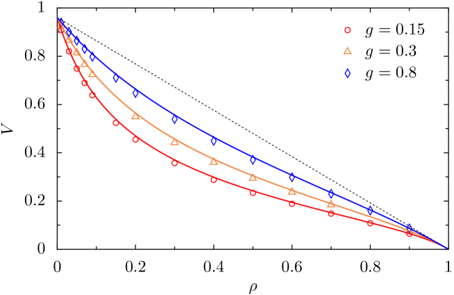
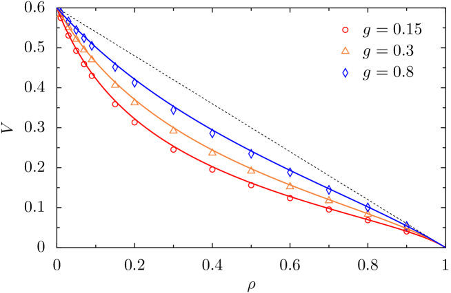
Refer to caption
Refer to caption
Figure 2: Stationary velocity V𝑉V of the TP as a function of the density for different values of the desorption rate g𝑔g obtained from numerical simulations (symbols) and from the decoupling approximation (lines). The bias is p1p1=0.96subscript𝑝1subscript𝑝10.96p_{1}-p_{-1}=0.96 (top) and p1p1=0.6subscript𝑝1subscript𝑝10.6p_{1}-p_{-1}=0.6 (bottom), the waiting times are τ=τ=1𝜏superscript𝜏1\tau=\tau^{*}=1. The dashed line is the trivial mean-field solution V=στ(p1p1)(1ρ)𝑉𝜎𝜏subscript𝑝1subscript𝑝11𝜌V=\frac{\sigma}{\tau}(p_{1}-p_{-1})(1-\rho).

6.3 Diffusion coefficient

6.3.1 Results

In a similar way, we study the diffusion coefficient as a function of the density ρ𝜌\rho, for different values of p1subscript𝑝1p_{1} and g𝑔g. We confront the analytical predictions to results from numerical simulations in Fig. 3. The dependence of the diffusion coefficient on the density of particles was first investigated in [31]. In the simulations results presented in that publication, the numerical errors were underestimated, and we present here refined results.
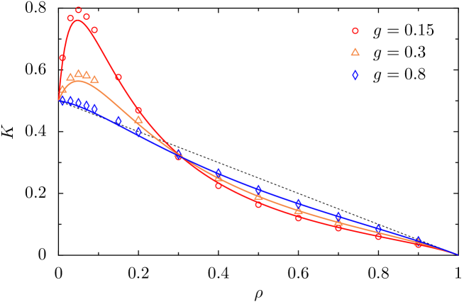
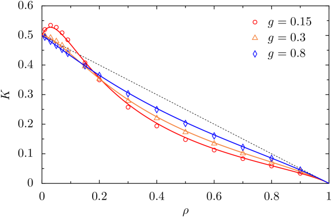
Refer to caption
Refer to caption
Figure 3: Stationary diffusion coefficient K𝐾K of the TP as a function of the density for different values of the desorption rate g𝑔g obtained from numerical simulations (symbols) and from the decoupling approximation (lines). The bias is p1p1=0.96subscript𝑝1subscript𝑝10.96p_{1}-p_{-1}=0.96 (top) and p1p1=0.6subscript𝑝1subscript𝑝10.6p_{1}-p_{-1}=0.6 (bottom), the waiting times are τ=τ=1𝜏superscript𝜏1\tau=\tau^{*}=1. The dashed line is the trivial mean-field solution K=σ22τ(1ρ)𝐾superscript𝜎22𝜏1𝜌K=\frac{\sigma^{2}}{2\tau}(1-\rho).

The analytical predictions as well as the numerical simulations reveal the existence of a striking effect: the diffusion coefficient can be a non-monotonic function of the density of bath particles. Conterintuitively, increasing the density of particles surrounding the TP may increase the TP diffusion coefficient in some range of parameters. This result is surprising, since one naturally expects that the diffusion coefficient will be maximal when there are no hardcore bath particles (i.e., when ρ=0𝜌0\rho=0). Consequently, this means that the diffusion of the TP may be enhanced by the presence of bath particles on the lattice. Moreover, we observe that for given values of p1subscript𝑝1p_{1} and g𝑔g, this extremum of the function K(ρ)𝐾𝜌K(\rho) may appear if the bias p1p1subscript𝑝1subscript𝑝1p_{1}-p_{-1} is large enough. This effect could be investigated in experimental situations (e.g. in microrheology) and could have interesting applications.

The discrepancy between the results from numerical simulations, which correspond to an exact sampling of the master equation (4), and the solution obtained using the decoupling approximations (Eqs. (12) and (26)) is small, except in the domain 0.05ρ0.15less-than-or-similar-to0.05𝜌less-than-or-similar-to0.150.05\lesssim\rho\lesssim 0.15. However, the approximate solution still gives a good qualitative description of the evolution of K𝐾K. The agreement is particularly good close to ρ=0𝜌0\rho=0 and ρ=1𝜌1\rho=1.

In what follows, we find the criterion on the parameters g𝑔g and p1subscript𝑝1p_{1} allowing the emergence of a maximum for K(ρ)𝐾𝜌K(\rho). In addition, we show that the non-monotonicity of the diffusion coefficient is actually correlated to the non-monotonicity of the cross-correlation functions g~nsubscript~𝑔𝑛\widetilde{g}_{n} in the domain n<0𝑛0n<0 (i.e. behind the TP).

6.3.2 Criterion for the existence of a maximum value of K𝐾K

In this section, we determine an explicit criterion for the existence of this maximum. This is equivalent to determine the parameters for which K(ρ)𝐾𝜌K(\rho) has a positive derivative at the origin. We will then solve the equation:

dKdρ|ρ=0=0.evaluated-atd𝐾d𝜌𝜌00\left.\frac{\mathrm{d}K}{\mathrm{d}\rho}\right|_{\rho=0}=0. (125)

If g𝑔g is fixed, as the density ρ𝜌\rho is related to f𝑓f and g𝑔g through ρ=f/(f+g)𝜌𝑓𝑓𝑔\rho=f/(f+g), this is equivalent to considering K𝐾K as a function of f𝑓f and solving

dKdf|f=0=0.evaluated-atd𝐾d𝑓𝑓00\left.\frac{\mathrm{d}K}{\mathrm{d}f}\right|_{f=0}=0. (126)

In what follows, we obtain the leading order term of K𝐾K in an expansion in powers of f𝑓f, the other parameters being constant. For simplicity, we introduce the quantities ττ/τsuperscript𝜏superscript𝜏𝜏\tau^{\prime}\equiv\tau^{*}/\tau and δp1p1𝛿subscript𝑝1subscript𝑝1\delta\equiv p_{1}-p_{-1}. Assuming that the quantities A±1subscript𝐴plus-or-minus1A_{\pm 1} have the following expansions

A±1=f0A±1(0)+A±1(1)f+𝒪(f2),subscript𝐴plus-or-minus1𝑓0subscriptsuperscript𝐴0plus-or-minus1subscriptsuperscript𝐴1plus-or-minus1𝑓𝒪superscript𝑓2A_{\pm 1}\underset{f\to 0}{=}A^{(0)}_{\pm 1}+A^{(1)}_{\pm 1}f+\mathcal{O}(f^{2}), (127)

and using Eqs. (89) and (90), we obtain

A±1=f01+(1±δ)ττg21±δ1+τ(1±δ)(δ2τ2+g(1+τ)±δδ2τ2+g2+2g(1+τ))f+𝒪(f2).subscript𝐴plus-or-minus1𝑓01plus-or-minus1𝛿superscript𝜏superscript𝜏superscript𝑔2plus-or-minus1𝛿1superscript𝜏plus-or-minus1𝛿plus-or-minussuperscript𝛿2superscriptsuperscript𝜏2𝑔1superscript𝜏𝛿superscript𝛿2superscriptsuperscript𝜏2superscript𝑔22𝑔1superscript𝜏𝑓𝒪superscript𝑓2A_{\pm 1}\underset{f\to 0}{=}1+(1\pm\delta)\tau^{\prime}-\frac{\tau^{\prime}}{g^{2}}\frac{1\pm\delta}{1+\tau^{\prime}(1\pm\delta)}\left(\delta^{2}{\tau^{\prime}}^{2}+g(1+\tau^{\prime})\pm\delta\sqrt{\delta^{2}{\tau^{\prime}}^{2}+g^{2}+2g(1+\tau^{\prime})}\right)f+\mathcal{O}(f^{2}). (128)

We can deduce from the expansions of A±1subscript𝐴plus-or-minus1A_{\pm 1} the expansions of K±subscript𝐾plus-or-minusK_{\pm}, r1subscript𝑟1r_{1} and r2subscript𝑟2r_{2} using Eqs. (85), (86) and (87). We then obtain the expansions of k±1subscript𝑘plus-or-minus1k_{\pm 1} and g~±1subscript~𝑔plus-or-minus1\widetilde{g}_{\pm 1} in powers of f𝑓f using the results from sections 5.1 and 5.2, and finally an expansion of K𝐾K with Eq. (52). These general expressions are too lengthy to be reproduced here, but we give them in the case τ=1superscript𝜏1\tau^{\prime}=1, which is the case we considered in our simulations:

K=f0σ22τ[1+N(g,δ)D(g,δ)f+𝒪(f2)]𝐾𝑓0superscript𝜎22𝜏delimited-[]1𝑁𝑔𝛿𝐷𝑔𝛿𝑓𝒪superscript𝑓2K\underset{f\to 0}{=}\frac{\sigma^{2}}{2\tau}\left[1+\frac{N(g,\delta)}{D(g,\delta)}f+\mathcal{O}(f^{2})\right] (129)

where

N(g,δ)=2[(δ24)g3+(3δ416)g2+δ2(3δ45δ2+4)g+δ4(δ43δ2+4)]𝑁𝑔𝛿2delimited-[]superscript𝛿24superscript𝑔33superscript𝛿416superscript𝑔2superscript𝛿23superscript𝛿45superscript𝛿24𝑔superscript𝛿4superscript𝛿43superscript𝛿24\displaystyle N(g,\delta)=2\left[(\delta^{2}-4)g^{3}+(3\delta^{4}-16)g^{2}+\delta^{2}(3\delta^{4}-5\delta^{2}+4)g+\delta^{4}(\delta^{4}-3\delta^{2}+4)\right]
δ2+g2+4g[2(δ44)(δ23)g2+δ2(δ4δ2+4)g+4δ4(δ22)],superscript𝛿2superscript𝑔24𝑔delimited-[]2superscript𝛿44superscript𝛿23superscript𝑔2superscript𝛿2superscript𝛿4superscript𝛿24𝑔4superscript𝛿4superscript𝛿22\displaystyle-\sqrt{\delta^{2}+g^{2}+4g}\left[2(\delta^{4}-4)(\delta^{2}-3)g^{2}+\delta^{2}(\delta^{4}-\delta^{2}+4)g+4\delta^{4}(\delta^{2}-2)\right], (130)
D(g,δ)=2(δ2)2(δ+2)2(δ2+g2+4g)g3.𝐷𝑔𝛿2superscript𝛿22superscript𝛿22superscript𝛿2superscript𝑔24𝑔superscript𝑔3\displaystyle D(g,\delta)=2(\delta-2)^{2}(\delta+2)^{2}(\delta^{2}+g^{2}+4g)g^{3}. (131)

For any value of δ𝛿\delta and g𝑔g, D(g,δ)>0𝐷𝑔𝛿0D(g,\delta)>0. For a given value of the bias δ𝛿\delta, the critical value of g𝑔g (denoted by gcsubscript𝑔cg_{\mathrm{c}}) allowing K𝐾K to reach a maximal value is then the solution of the equation:

N(gc,δ)=0,𝑁subscript𝑔c𝛿0N(g_{\mathrm{c}},\delta)=0, (132)

which can be determined numerically. We present the numerical solutions of Eq. (132) in Fig. 4 (curves in blue). On this figure, we also give the solutions obtained for other values of τsuperscript𝜏\tau^{\prime}. We conclude that, for a fixed value of the bias, K𝐾K is nonmonotonic if the desorption rate g𝑔g is large enough (or, for a fixed value of the desorption rate, if the bias is large enough).
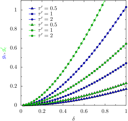
Refer to caption
Figure 4: Critical value of the desorption rate gcsubscript𝑔cg_{\mathrm{c}} as a function of δ𝛿\delta, for different values of the ratio τ=τ/τsuperscript𝜏superscript𝜏𝜏\tau^{\prime}=\tau^{*}/\tau, with σ=1𝜎1\sigma=1 and τ=1𝜏1\tau=1 obtained by the study of the behavior of K𝐾K at ρ0𝜌0\rho\to 0 (curves in blue). The region below the curves correspond to the range of parameters where K(ρ)𝐾𝜌K(\rho) is nonmonotonic. The critical value of the desorption rate gcsubscriptsuperscript𝑔cg^{\prime}_{\mathrm{c}} for which the cross-correlations g~~𝑔\widetilde{g} have the property g~1>g~2subscript~𝑔1subscript~𝑔2\widetilde{g}_{-1}>\widetilde{g}_{-2} is represented in green. The region below the curves correspond to the range of parameters where g~1>g~2subscript~𝑔1subscript~𝑔2\widetilde{g}_{-1}>\widetilde{g}_{-2}.

6.3.3 Influence of the cross-correlations functions on the non-monotonicity

We now aim to give a first insight into a better understanding of the non-monotonicity of the diffusion coefficient. We first notice that the diffusion coefficient K𝐾K (Eq. (52)) may be separated into three contributions:

K=KMF+K1+K2,𝐾subscript𝐾MFsubscript𝐾1subscript𝐾2K=K_{\rm MF}+K_{1}+K_{2}, (133)

with

KMFsubscript𝐾MF\displaystyle K_{\rm MF} =\displaystyle= σ2τ(1ρ),superscript𝜎2𝜏1𝜌\displaystyle\frac{\sigma^{2}}{\tau}(1-\rho), (134)
K1subscript𝐾1\displaystyle K_{1} =\displaystyle= σ2τ[p1(k1ρ)+p1(k1ρ)],superscript𝜎2𝜏delimited-[]subscript𝑝1subscript𝑘1𝜌subscript𝑝1subscript𝑘1𝜌\displaystyle-\frac{\sigma^{2}}{\tau}[p_{1}(k_{1}-\rho)+p_{-1}(k_{-1}-\rho)], (135)
K2subscript𝐾2\displaystyle K_{2} =\displaystyle= 2στ(p1g~1p1g~1).2𝜎𝜏subscript𝑝1subscript~𝑔1subscript𝑝1subscript~𝑔1\displaystyle-\frac{2\sigma}{\tau}(p_{1}\widetilde{g}_{1}-p_{-1}\widetilde{g}_{-1}). (136)

The first term is the trivial mean-field approximation of the problem, obtained by taking the average local densities k𝒓subscript𝑘𝒓k_{\boldsymbol{r}} equal to ρ𝜌\rho and the cross-correlation functions g~𝒓=δXtδηXt+𝒓subscript~𝑔𝒓delimited-⟨⟩𝛿subscript𝑋𝑡𝛿subscript𝜂subscript𝑋𝑡𝒓\widetilde{g}_{\boldsymbol{r}}=\left\langle\delta X_{t}\delta\eta_{X_{t}+\boldsymbol{r}}\right\rangle equal to zero. K1subscript𝐾1K_{1} may be seen as a contribution from the inhomogeneous density profiles, and K2subscript𝐾2K_{2} a contribution from the cross-correlations g~±1subscript~𝑔plus-or-minus1\widetilde{g}_{\pm 1}. For a given set of parameters which gives rise to a non-monotonic behavior (p1=0.98subscript𝑝10.98p_{1}=0.98 and g=0.15𝑔0.15g=0.15), we plot in Fig. 5 K𝐾K as well as the three contributions. The origin of the non-monotonicity of K𝐾K with respect to the density ρ𝜌\rho can then be attributed to K2subscript𝐾2K_{2}.

Refer to caption
Figure 5: Contributions in the expressions of K𝐾K as a function of the density, for the parameters p1=0.98subscript𝑝10.98p_{1}=0.98 and g=0.15𝑔0.15g=0.15.

The cross-correlation functions g~nsubscript~𝑔𝑛\widetilde{g}_{n} have nontrivial behaviors with respect to the distance n𝑛n to the TP. In particular, they appear to have a non-monotonous behavior in the domain n<0𝑛0n<0, i.e. behind the TP, for some values of the parameters. On Fig. 6, we plot the functions g~nsubscript~𝑔𝑛\widetilde{g}_{n} for different values of the density ρ𝜌\rho, for two sets of parameters: one for which the diffusion K𝐾K is known to be a non-monotonic function of the density (p1=0.98subscript𝑝10.98p_{1}=0.98 and g=0.2𝑔0.2g=0.2), and one for which it is monotonic (p1=0.98subscript𝑝10.98p_{1}=0.98 and g=0.6𝑔0.6g=0.6). On Fig. 7, we plot the functions g~nsubscript~𝑔𝑛\widetilde{g}_{n} for different values of the desorption parameter g𝑔g, for ρ=0.01𝜌0.01\rho=0.01, for p1=0.98subscript𝑝10.98p_{1}=0.98. The non-monotonicity of g~nsubscript~𝑔𝑛\widetilde{g}_{n} with the distance to the TP then seems to be correlated with that of K𝐾K with the density, as it occurs for g𝑔g small enough.

Refer to caption
Figure 6: Cross-correlations functions g~~𝑔\widetilde{g} as a function of the distance to the tracer n𝑛n for g=0.2𝑔0.2g=0.2 (left) and g=0.6𝑔0.6g=0.6 (right), and for different values of the density ρ𝜌\rho. In both cases, p1=0.98subscript𝑝10.98p_{1}=0.98.
Refer to caption
Figure 7: Cross-correlations functions g~~𝑔\widetilde{g} as a function of the distance to the tracer n𝑛n for ρ=0.01𝜌0.01\rho=0.01, p1=0.98subscript𝑝10.98p_{1}=0.98, and for different values of the desorption parameter g𝑔g.

In order to get a more quantitative comparison of these two effects (the non-monotonicity of K𝐾K with respect to the density ρ𝜌\rho and that of g~nsubscript~𝑔𝑛\widetilde{g}_{n} with respect to the distance to the TP n𝑛n in the domain n<0𝑛0n<0), we first determine, for a fixed value of the bias p1p1subscript𝑝1subscript𝑝1p_{1}-p_{-1}, and at leading order in f𝑓f, the critical value of gcsubscriptsuperscript𝑔cg^{\prime}_{\rm c} giving a non-monotonic behavior for g~nsubscript~𝑔𝑛\widetilde{g}_{n}, i.e. for which g~1>g~2subscript~𝑔1subscript~𝑔2\widetilde{g}_{-1}>\widetilde{g}_{-2}.

Using the small f𝑓f expansion of A±1subscript𝐴plus-or-minus1A_{\pm 1} (Eq. (128)), we easily deduce from the definitions of g~nsubscript~𝑔𝑛\widetilde{g}_{n} in the domain n<0𝑛0n<0 (Eq. (96)) an expression for g~1g~2subscript~𝑔1subscript~𝑔2\widetilde{g}_{-1}-\widetilde{g}_{-2} at leading order in f𝑓f. The general expression is too lengthy to be given here. We present it in the particular case where τ=1superscript𝜏1\tau^{\prime}=1:

g~1g~2=f02σfN(g,δ)D(g,δ)+𝒪(f2)subscript~𝑔1subscript~𝑔2𝑓02𝜎𝑓superscript𝑁𝑔𝛿superscript𝐷𝑔𝛿𝒪superscript𝑓2\widetilde{g}_{-1}-\widetilde{g}_{-2}\underset{f\to 0}{=}2\sigma f\frac{N^{\prime}(g,\delta)}{D^{\prime}(g,\delta)}+\mathcal{O}(f^{2}) (137)

with

N(g,δ)=superscript𝑁𝑔𝛿absent\displaystyle N^{\prime}(g,\delta)= (δg)[(1+δ)g22(δ22δ2)g+δ2(δ1)]𝛿𝑔delimited-[]1𝛿superscript𝑔22superscript𝛿22𝛿2𝑔superscript𝛿2𝛿1\displaystyle(\delta-g)\left[(1+\delta)g^{2}-2(\delta^{2}-2\delta-2)g+\delta^{2}(\delta-1)\right]
δ2+g2+4g[(1+δ)g2(3δ+2)(δ1)g+δ2(δ1)],superscript𝛿2superscript𝑔24𝑔delimited-[]1𝛿superscript𝑔23𝛿2𝛿1𝑔superscript𝛿2𝛿1\displaystyle-\sqrt{\delta^{2}+g^{2}+4g}\left[(1+\delta)g^{2}-(3\delta+2)(\delta-1)g+\delta^{2}(\delta-1)\right], (138)
D(g,δ)=superscript𝐷𝑔𝛿absent\displaystyle D^{\prime}(g,\delta)= 2gδ2+g2+4g{[2g2+(2δ+4)g+δ(δ+2)]δ2+g2+4g\displaystyle 2g\sqrt{\delta^{2}+g^{2}+4g}\Big{\{}\left[2g^{2}+(2\delta+4)g+\delta(\delta+2)\right]\sqrt{\delta^{2}+g^{2}+4g}
+2g3+2(δ+4)g2+2(δ+2)(δ+1)g+δ2(δ+2)}.\displaystyle+2g^{3}+2(\delta+4)g^{2}+2(\delta+2)(\delta+1)g+\delta^{2}(\delta+2)\Big{\}}. (139)

Then, for a fixed value of the bias δ𝛿\delta, the critical value of g𝑔g canceling g~1g~2subscript~𝑔1subscript~𝑔2\widetilde{g}_{-1}-\widetilde{g}_{-2} is the solution of the equation

N(gc,δ)=0.superscript𝑁subscriptsuperscript𝑔c𝛿0N^{\prime}(g^{\prime}_{\rm c},\delta)=0. (140)

The numerical solutions for gcsubscriptsuperscript𝑔cg^{\prime}_{\rm c} as a function of δ𝛿\delta, for different values of the ratio τsuperscript𝜏\tau^{\prime} are represented in Fig. 4 and confronted to the values gcsubscript𝑔cg_{\rm c} obtained by the criterion on K𝐾K. The two functions gcsubscript𝑔cg_{\rm c} and gcsubscriptsuperscript𝑔cg^{\prime}_{\rm c} are comparable as long as τsuperscript𝜏\tau^{\prime} is not too large. We also show that their expansions for δ0𝛿0\delta\to 0 are identical at leading order, and that they go to zero as (17+1)δ2/8171superscript𝛿28(\sqrt{17}+1)\delta^{2}/8.

This study indicates that the emergence of a maximal value for K(ρ)𝐾𝜌K(\rho) for ρ>0𝜌0\rho>0 is correlated to the observation of a minimal value in the cross-correlation functions g~nsubscript~𝑔𝑛\widetilde{g}_{n} in the domain n<0𝑛0n<0.

In G, for given values of the jump probability p1subscript𝑝1p_{1} and of the desorption parameter g𝑔g, we study the range of density [0,ρ~]0~𝜌[0,\widetilde{\rho}] for which the diffusion coefficient is greater than 1/2121/2, which is its value when there is no bath particle. We also determine the range of density [0,ρ~]0superscript~𝜌[0,\widetilde{\rho}^{\prime}] for which g~1g~2<0subscript~𝑔1subscript~𝑔20\widetilde{g}_{-1}-\widetilde{g}_{-2}<0. The range of parameters for which K>1/2𝐾12K>1/2 is then shown to be correlated to the range of parameters for which g~1g~2<0subscript~𝑔1subscript~𝑔20\widetilde{g}_{-1}-\widetilde{g}_{-2}<0.

These two studies (from sections 6.3.3 and G) show that the non-monotonicity of the diffusion coefficient with respect to the density (emergence of a maximum value of K𝐾K for ρ>0𝜌0\rho>0) and the non-monotonicity of the cross-correlation function g~nsubscript~𝑔𝑛\widetilde{g}_{n} behind the TP are correlated. A more detailed study of the cross-correlation functions g~nsubscript~𝑔𝑛\widetilde{g}_{n}, whose behavior affects the fluctuations of the TP position, could allow us to have a more physical understanding of the phenomenon highlighted in this section.

6.4 Third cumulant

The third cumulant of the distribution of Xtsubscript𝑋𝑡X_{t} gives information about its asymmetry. We introduced earlier the coefficient γ𝛾\gamma, defined by

γ=limt16ddt(XtXt)3.𝛾subscript𝑡16dd𝑡delimited-⟨⟩superscriptsubscript𝑋𝑡delimited-⟨⟩subscript𝑋𝑡3\gamma=\lim_{t\to\infty}\frac{1}{6}\frac{\mathrm{d}}{\mathrm{d}t}\left\langle({X_{t}}-\left\langle X_{t}\right\rangle)^{3}\right\rangle. (141)

With this definition, if γ>0𝛾0\gamma>0 (resp. γ<0𝛾0\gamma<0), the distribution of Xtsubscript𝑋𝑡X_{t} is expected to be skewed to the right (resp. to the left). Let us recall the situation of a biased random walker on a lattice in the absence of exclusion interactions. If the particle is more likely to jump to the right (p1>p1subscript𝑝1subscript𝑝1p_{1}>p_{-1}), its third cumulant will be positive, indicating a distribution skewed to the right. Here, we study the influence of the presence of bath particles and of the different parameters of our model on the sign of the third cumulant of Xtsubscript𝑋𝑡X_{t}.

We use the solutions for m~±1subscript~𝑚plus-or-minus1\widetilde{m}_{\pm 1} (Eqs. (112) and (113)) obtained from the decoupling approximation in order to compute the coefficient γ𝛾\gamma from its definition (Eq. (81)). For two values of the bias (p1=0.98subscript𝑝10.98p_{1}=0.98 and 0.80.80.8), we study the coefficient γ𝛾\gamma as a function of the density ρ𝜌\rho, for different values of the desorption rate g𝑔g. The solutions of the equations obtained from the decoupling approximation are compared to results from numerical simulations. The curves are presented in Fig. 8. For high values of the desorption rate, γ(ρ)𝛾𝜌\gamma(\rho) is monotonic and decreases when the density of bath particles increases. However, for small values of the desorption rate, the function becomes nonmonotonic, and one observes the emergence of a minimum and a maximum value, different from the trivial extrema at ρ=0𝜌0\rho=0 and ρ=1𝜌1\rho=1. Finally, if g𝑔g is small enough, there exists an interval of density for which γ𝛾\gamma becomes negative, which means that the distribution of Xtsubscript𝑋𝑡X_{t} may actually be negatively skewed, in opposition with the situation where there is no bath particles on the lattice.

Confronting these predictions with results from numerical simulations, we show that the decoupling approximation offers a good prediction of the behavior of the third cumulant of the TP position in a wide range of parameters.
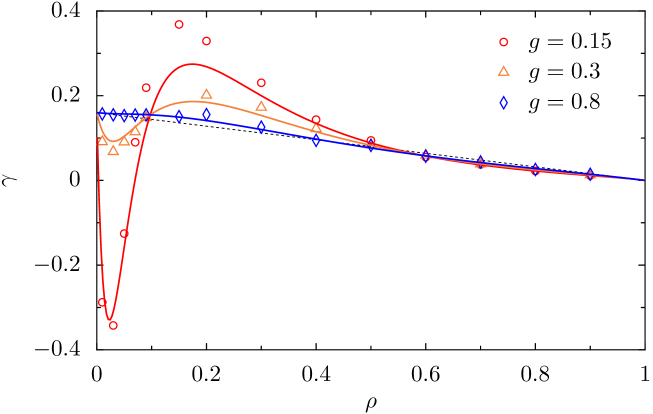
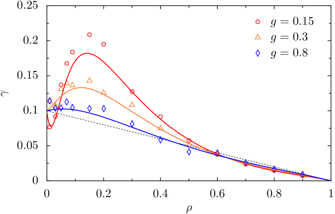
Refer to caption
Refer to caption
Figure 8: Coefficient γ𝛾\gamma defined in Eq. (141) as a function of the density for different values of the desorption rate g𝑔g obtained from the decoupling approximation. The bias is p1p1=0.96subscript𝑝1subscript𝑝10.96p_{1}-p_{-1}=0.96 (top) and p1p1=0.6subscript𝑝1subscript𝑝10.6p_{1}-p_{-1}=0.6 (bottom). The waiting times are τ=τ=1𝜏superscript𝜏1\tau=\tau^{*}=1. The dashed lines are the trivial mean-field solutions: σ36τ(p1p1)(1ρ)superscript𝜎36𝜏subscript𝑝1subscript𝑝11𝜌\frac{\sigma^{3}}{6\tau}(p_{1}-p_{-1})(1-\rho).

6.5 Cumulant generating function and propagator

For a given set of parameters, we solve the system of equations which determines w~±1subscript~𝑤plus-or-minus1\widetilde{w}_{\pm 1} implicitly (Eq. (124)), and we obtain the numerical values of w~±1(u)subscript~𝑤plus-or-minus1𝑢\widetilde{w}_{\pm 1}(u) for u𝑢u varying in [π,π]𝜋𝜋[-\pi,\pi]. We represent the real and imaginary parts of w~±1(u)subscript~𝑤plus-or-minus1𝑢\widetilde{w}_{\pm 1}(u) as functions of u𝑢u in Fig. 9. The p.d.f. Pt(x)subscript𝑃𝑡𝑥P_{t}(x) in the long-time limit is obtained from Eq. (65).
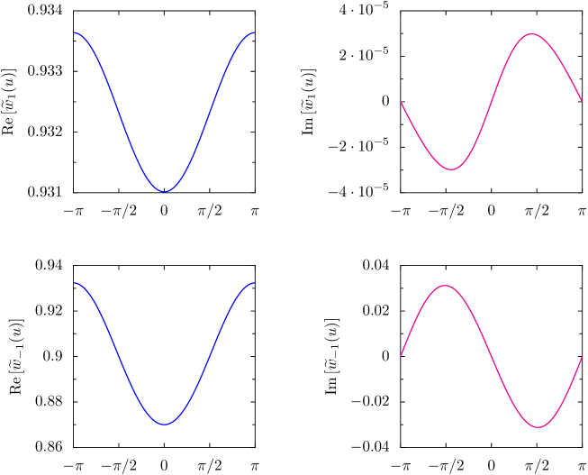
Refer to caption
Figure 9: Real and imaginary parts of the generalized correlation functions w~±1(u)subscript~𝑤plus-or-minus1𝑢\widetilde{w}_{\pm 1}(u), obtained from the resolution of the system (124), for the parameters ρ=0.9𝜌0.9\rho=0.9, g=0.15𝑔0.15g=0.15, p1=0.98subscript𝑝10.98p_{1}=0.98, τ=τ=σ=1𝜏superscript𝜏𝜎1\tau=\tau^{*}=\sigma=1.

We compare the results from this calculation with data obtained from Monte Carlo simulations for a given set of parameters (see Fig. 10).
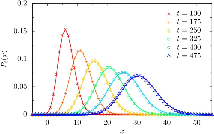
Refer to caption
Figure 10: Probability distribution function of the TP position Pt(x)=Prob[Xt=x]subscript𝑃𝑡𝑥Probdelimited-[]subscript𝑋𝑡𝑥P_{t}(x)=\mathrm{Prob}[X_{t}=x], for different times. The results from numerical simulations (symbols) are compared to the expression (65), the functions w~±1(u)subscript~𝑤plus-or-minus1𝑢\widetilde{w}_{\pm 1}(u) being numerically computed as solutions of the system (124). The parameters are g=0.15𝑔0.15g=0.15, p1=0.98subscript𝑝10.98p_{1}=0.98, ρ=0.9𝜌0.9\rho=0.9.

We observe a good agreement between the analytical prediction obtained from the decoupling approximation and the results from numerical simulations. We see that the prediction from the decoupling approximation tends to be shifted to the right for large times: this is expected from the analysis of the velocity of the TP, which was shown to be overestimated by the approximation (Fig. 2).

As emphasized in section 4.1, the rescaled variable Zt=(XtXt)/Var(Xt)subscript𝑍𝑡subscript𝑋𝑡delimited-⟨⟩subscript𝑋𝑡Varsubscript𝑋𝑡Z_{t}=(X_{t}-\left\langle X_{t}\right\rangle)/\sqrt{\mathrm{Var}(X_{t})} is expected to be distributed accordingly to a Gaussian distribution in the long-time limit. We plot on Fig. 11 the distribution 𝒫𝒫\mathcal{P} defined by

𝒫t(z)=Prob[Zt=z],subscript𝒫𝑡𝑧Probdelimited-[]subscript𝑍𝑡𝑧\mathcal{P}_{t}(z)=\mathrm{Prob}\left[Z_{t}=z\right], (142)

and compare it with the normal distribution ex2/2/2πsuperscriptesuperscript𝑥222𝜋\mathrm{e}^{-x^{2}/2}/\sqrt{2\pi}. At sufficiently long times, the distribution of the random variable Ztsubscript𝑍𝑡Z_{t} converges to the normal distribution of mean zero and unit variance. The rescaled position of the TP is then asymptotically Gaussian in the long-time limit.
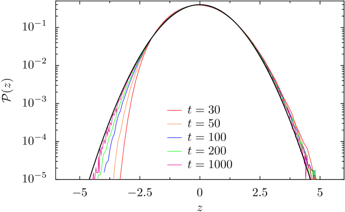
Refer to caption
Figure 11: Probability distribution of the rescaled variable Zt=(XtXt)/Var(Xt)subscript𝑍𝑡subscript𝑋𝑡delimited-⟨⟩subscript𝑋𝑡Varsubscript𝑋𝑡Z_{t}=(X_{t}-\left\langle X_{t}\right\rangle)/\sqrt{\mathrm{Var}(X_{t})} at different times, obtained with the following parameters: ρ=0.1𝜌0.1\rho=0.1, g=0.15𝑔0.15g=0.15, p1=0.98subscript𝑝10.98p_{1}=0.98, τ=τ=σ=1𝜏superscript𝜏𝜎1\tau=\tau^{*}=\sigma=1. The black line is the normal distribution exp(x2/2)/2πsuperscript𝑥222𝜋\exp(-x^{2}/2)/\sqrt{2\pi}.

7 Conclusion

We studied the diffusion of a biased tracer particle (TP) in a hardcore lattice gas in contact with a reservoir of particles. From the general master equation of the problem, we gave a detailed derivation of the equation satisfied by the fluctuations of the position of the TP and presented in a previous publication. This equation involve the density profiles around the TP and cross-correlation functions, whose evolution equations are obtained in a closed form by resorting to mean-field type approximation.

Going one step further, we extended this approximation to higher-order correlation functions in order to obtain the evolution equation verified by the cumulant generating function of the TP position. This equation then yields the entire probability distribution of the TP on a lattice of arbitrary dimension. We also obtained the equation satisfied by the third-cumulant of the distribution, which gives information about its asymmetry.

We then solved these equations in the particular case of a one-dimensional lattice. We recall the result from [31]: the diffusion coefficient of the TP is a nonmonotonic function of the density of bath particles. Counterintuitively, it reaches a maximum value for a nonzero value of the density. Thus, the presence of bath particles on the lattice may actually enhance its diffusion coefficient. Here, we showed that this effect is related to an anomaly in the behavior of bath-tracer cross-correlation functions, that are nonmonotonic functions of the distance to the TP. Another surprising observation arises by analyzing the third cumulant of the TP position, which was shown to be nonmonotonic and to take negative values in a wide range of parameters. These analytical predictions were confronted with exact numerical samplings of the master equation, which indicate that the approximation we used is accurate in a wide range of parameters.

We finally solved the equation satisfied by the cumulant generating function, deduced the probability distribution and showed that the position of the TP rescaled by its fluctuations is Gaussian-distributed in the long-time limit.

The equations presented in this paper are very general, and allow to compute the cumulants of the TP position and therefore its distribution under a mean-field-type approximation which was shown to be accurate in a broad range of parameters. These equations are valid for lattices of arbitrary dimension. We leave to future work the study of their solutions on higher-dimensional lattices. It could be interesting to see if the results obtained on the one-dimensional lattice – enhanced diffusion coefficient, nonmonotonic and negative third cumulant, convergence of the rescaled distribution to a Gaussian distribution – can be extended to lattices of higher dimension, or observed in experimental systems.

Acknowledgments

OB acknowledges financial support from the European Research Council Starting Grant FPTOpt-277998.

Appendix A Evolution equations of Xt2delimited-⟨⟩superscriptsubscript𝑋𝑡2\left\langle{X_{t}}^{2}\right\rangle

In this appendix, we give an explicit derivation of Eq. (19), which governs the evolution of the second moment of Xtsubscript𝑋𝑡X_{t}. We multiply the master equation (4) by (𝑿𝒆1)2superscript𝑿subscript𝒆12(\boldsymbol{X}\cdot\boldsymbol{e}_{1})^{2} and average over all the bath configurations η𝜂\eta and all the positions of the TP 𝑿𝑿\boldsymbol{X}. We consider separately each term of the master equation:

  • the left-hand-side term of (4) gives the contribution:

    CLsubscript𝐶L\displaystyle C_{\mathrm{L}} =\displaystyle= 𝑿,η(𝑿𝒆1)22dτtP(𝑿,η;t)subscript𝑿𝜂superscript𝑿subscript𝒆122𝑑superscript𝜏subscript𝑡𝑃𝑿𝜂𝑡\displaystyle\sum_{\boldsymbol{X},\eta}(\boldsymbol{X}\cdot\boldsymbol{e}_{1})^{2}2d\tau^{*}\partial_{t}P(\boldsymbol{X},\eta;t) (143)
    =\displaystyle= 2dτt(𝑿,η(𝑿𝒆1)2P(𝑿,η;t))2𝑑superscript𝜏subscript𝑡subscript𝑿𝜂superscript𝑿subscript𝒆12𝑃𝑿𝜂𝑡\displaystyle 2d\tau^{*}\partial_{t}\left(\sum_{\boldsymbol{X},\eta}(\boldsymbol{X}\cdot\boldsymbol{e}_{1})^{2}P(\boldsymbol{X},\eta;t)\right) (144)
    =\displaystyle= 2dτdXt2dt2𝑑superscript𝜏ddelimited-⟨⟩superscriptsubscript𝑋𝑡2d𝑡\displaystyle 2d\tau^{*}\frac{\mathrm{d}\left\langle{X_{t}}^{2}\right\rangle}{\mathrm{d}t} (145)
  • the first term of the right-hand-side yields

    C1=𝑿,η(𝑿𝒆1)2μ=1d𝒓𝑿𝒆μ,𝑿[P(𝑿,η𝒓,μ;t)P(𝑿,η;t)]subscript𝐶1subscript𝑿𝜂superscript𝑿subscript𝒆12superscriptsubscript𝜇1𝑑subscript𝒓𝑿subscript𝒆𝜇𝑿delimited-[]𝑃𝑿superscript𝜂𝒓𝜇𝑡𝑃𝑿𝜂𝑡\displaystyle C_{1}=\sum_{\boldsymbol{X},\eta}(\boldsymbol{X}\cdot\boldsymbol{e}_{1})^{2}\sum_{\mu=1}^{d}\sum_{{\boldsymbol{r}}\neq\boldsymbol{X}-\boldsymbol{e}_{\mu},\boldsymbol{X}}\left[P(\boldsymbol{X},\eta^{{\boldsymbol{r}},\mu};t)-P(\boldsymbol{X},\eta;t)\right] (146)
    =𝑿(𝑿𝒆1)2μ=1d𝒓𝑿𝒆μ,𝑿η[P(𝑿,η𝒓,μ;t)P(𝑿,η;t)].absentsubscript𝑿superscript𝑿subscript𝒆12superscriptsubscript𝜇1𝑑subscript𝒓𝑿subscript𝒆𝜇𝑿subscript𝜂delimited-[]𝑃𝑿superscript𝜂𝒓𝜇𝑡𝑃𝑿𝜂𝑡\displaystyle=\sum_{\boldsymbol{X}}(\boldsymbol{X}\cdot\boldsymbol{e}_{1})^{2}\sum_{\mu=1}^{d}\sum_{{\boldsymbol{r}}\neq\boldsymbol{X}-\boldsymbol{e}_{\mu},\boldsymbol{X}}\sum_{\eta}\left[P(\boldsymbol{X},\eta^{{\boldsymbol{r}},\mu};t)-P(\boldsymbol{X},\eta;t)\right]. (147)

    Recalling that η𝒓,μsuperscript𝜂𝒓𝜇\eta^{{\boldsymbol{r}},\mu} a configuration obtained from η𝜂\eta by exchanging the occupation variables of two neighboring sites 𝒓𝒓{\boldsymbol{r}} and 𝒓+𝒆μ𝒓subscript𝒆𝜇\boldsymbol{r}+\boldsymbol{e}_{\mu}, we obtain

    ηP(𝑿,η𝒓,μ;t)=ηP(𝑿,η;t),subscript𝜂𝑃𝑿superscript𝜂𝒓𝜇𝑡subscript𝜂𝑃𝑿𝜂𝑡\sum_{\eta}P(\boldsymbol{X},\eta^{{\boldsymbol{r}},\mu};t)=\sum_{\eta}P(\boldsymbol{X},\eta;t), (148)

    and we conclude that C1=0subscript𝐶10C_{1}=0.

  • the second term of the right-hand-side of Eq. (4) gives the contribution:

    C2=subscript𝐶2absent\displaystyle C_{2}= 2dττμpμ[𝑿,η(𝑿𝒆1)2(1η𝑿)P(𝑿𝒆𝝁,η;t)\displaystyle\frac{2d\tau^{*}}{\tau}\sum_{\mu}p_{\mu}\left[\sum_{\boldsymbol{X},\eta}(\boldsymbol{X}\cdot\boldsymbol{e}_{1})^{2}\left(1-\eta_{\boldsymbol{X}}\right)P(\boldsymbol{X}-\boldsymbol{e}_{\boldsymbol{\mu}},\eta;t)\right.
    𝑿,η(𝑿𝒆1)2(1η𝑿+𝒆μ)P(𝑿,η;t)].\displaystyle\left.-\sum_{\boldsymbol{X},\eta}(\boldsymbol{X}\cdot\boldsymbol{e}_{1})^{2}\left(1-\eta_{\boldsymbol{X}+\boldsymbol{e}_{\mu}}\right)P(\boldsymbol{X},\eta;t)\right]. (149)

    We consider for instance the term corresponding to μ=1𝜇1\mu=1, and consider the first sum over 𝑿𝑿\boldsymbol{X} and η𝜂\eta, in which we make the change of variable 𝑿𝑿+𝒆1𝑿𝑿subscript𝒆1\boldsymbol{X}\leftarrow\boldsymbol{X}+\boldsymbol{e}_{1}:

    𝑿,η(𝑿𝒆1)2(1η𝑿)P(𝑿𝒆1,η;t)subscript𝑿𝜂superscript𝑿subscript𝒆121subscript𝜂𝑿𝑃𝑿subscript𝒆1𝜂𝑡\displaystyle\sum_{\boldsymbol{X},\eta}(\boldsymbol{X}\cdot\boldsymbol{e}_{1})^{2}\left(1-\eta_{\boldsymbol{X}}\right)P(\boldsymbol{X}-\boldsymbol{e}_{1},\eta;t) (150)
    =𝑿,η(𝑿𝒆1+σ)2(1η𝑿+𝒆1)P(𝑿,η;t)absentsubscript𝑿𝜂superscript𝑿subscript𝒆1𝜎21subscript𝜂𝑿subscript𝒆1𝑃𝑿𝜂𝑡\displaystyle=\sum_{\boldsymbol{X},\eta}(\boldsymbol{X}\cdot\boldsymbol{e}_{1}+\sigma)^{2}\left(1-\eta_{\boldsymbol{X}+\boldsymbol{e}_{1}}\right)P(\boldsymbol{X},\eta;t) (151)
    =𝑿,η[(𝑿𝒆1)2+σ2+2σ(𝑿𝒆1)]2(1η𝑿+𝒆1)P(𝑿,η;t).absentsubscript𝑿𝜂superscriptdelimited-[]superscript𝑿subscript𝒆12superscript𝜎22𝜎𝑿subscript𝒆121subscript𝜂𝑿subscript𝒆1𝑃𝑿𝜂𝑡\displaystyle=\sum_{\boldsymbol{X},\eta}[(\boldsymbol{X}\cdot\boldsymbol{e}_{1})^{2}+\sigma^{2}+2\sigma(\boldsymbol{X}\cdot\boldsymbol{e}_{1})]^{2}\left(1-\eta_{\boldsymbol{X}+\boldsymbol{e}_{1}}\right)P(\boldsymbol{X},\eta;t). (152)

    Finally, we get

    𝑿,η(𝑿𝒆1)2(1η𝑿)P(𝑿𝒆μ,η;t)𝑿,η(𝑿𝒆1)2(1η𝑿+𝒆μ)P(𝑿,η;t)subscript𝑿𝜂superscript𝑿subscript𝒆121subscript𝜂𝑿𝑃𝑿subscript𝒆𝜇𝜂𝑡subscript𝑿𝜂superscript𝑿subscript𝒆121subscript𝜂𝑿subscript𝒆𝜇𝑃𝑿𝜂𝑡\displaystyle\sum_{\boldsymbol{X},\eta}(\boldsymbol{X}\cdot\boldsymbol{e}_{1})^{2}\left(1-\eta_{\boldsymbol{X}}\right)P(\boldsymbol{X}-\boldsymbol{e}_{\mu},\eta;t)-\sum_{\boldsymbol{X},\eta}(\boldsymbol{X}\cdot\boldsymbol{e}_{1})^{2}\left(1-\eta_{\boldsymbol{X}+\boldsymbol{e}_{\mu}}\right)P(\boldsymbol{X},\eta;t) (153)
    =σ2𝑿,η(1η𝑿+𝒆1)P(𝑿,η;t)+2σ𝑿,η(𝑿𝒆1)(1η𝑿+𝒆1)P(𝑿,η;t).absentsuperscript𝜎2subscript𝑿𝜂1subscript𝜂𝑿subscript𝒆1𝑃𝑿𝜂𝑡2𝜎subscript𝑿𝜂𝑿subscript𝒆11subscript𝜂𝑿subscript𝒆1𝑃𝑿𝜂𝑡\displaystyle=\sigma^{2}\sum_{\boldsymbol{X},\eta}(1-\eta_{\boldsymbol{X}+\boldsymbol{e}_{1}})P(\boldsymbol{X},\eta;t)+2\sigma\sum_{\boldsymbol{X},\eta}(\boldsymbol{X}\cdot\boldsymbol{e}_{1})(1-\eta_{\boldsymbol{X}+\boldsymbol{e}_{1}})P(\boldsymbol{X},\eta;t). (154)

    Following the same procedure for the term μ=1𝜇1\mu=-1 and noticing that the terms obtained for μ=±2,,±d𝜇plus-or-minus2plus-or-minus𝑑\mu=\pm 2,\dots,\pm d in (149) cancel, we finally get

    C2=subscript𝐶2absent\displaystyle C_{2}= 2dττ{p1[σ2(1k𝒆1(t))+2σ(Xtg𝒆1(t))]\displaystyle\frac{2d\tau^{*}}{\tau}\left\{p_{1}[\sigma^{2}(1-k_{\boldsymbol{e}_{1}}(t))+2\sigma(\left\langle X_{t}\right\rangle-g_{\boldsymbol{e}_{1}}(t))]\right.
    +p1[σ2(1k𝒆1(t))2σ(Xtg𝒆1(t))]},\displaystyle+\left.p_{-1}[\sigma^{2}(1-k_{\boldsymbol{e}_{-1}}(t))-2\sigma(\left\langle X_{t}\right\rangle-g_{\boldsymbol{e}_{-1}}(t))]\right\}, (155)

    where we define

    g𝒓(t)=Xtη𝑿t+𝒓.subscript𝑔𝒓𝑡delimited-⟨⟩subscript𝑋𝑡subscript𝜂subscript𝑿𝑡𝒓g_{\boldsymbol{r}}(t)=\left\langle X_{t}\eta_{\boldsymbol{X}_{t}+\boldsymbol{r}}\right\rangle. (156)
  • the third term of the right-hand-side of Eq. (4) yields

    C3=subscript𝐶3absent\displaystyle C_{3}= 2dg𝑿,η(𝑿𝒆1)2𝒓𝑿[(1η𝒓)P(𝑿,η^𝒓;t)η𝒓P(𝑿,η;t)]2𝑑𝑔subscript𝑿𝜂superscript𝑿subscript𝒆12subscript𝒓𝑿delimited-[]1subscript𝜂𝒓𝑃𝑿superscript^𝜂𝒓𝑡subscript𝜂𝒓𝑃𝑿𝜂𝑡\displaystyle 2dg\sum_{\boldsymbol{X},\eta}(\boldsymbol{X}\cdot\boldsymbol{e}_{1})^{2}\sum_{{\boldsymbol{r}}\neq\boldsymbol{X}}\left[\left(1-\eta_{\boldsymbol{r}}\right)P(\boldsymbol{X},\hat{\eta}^{{\boldsymbol{r}}};t)-\eta_{\boldsymbol{r}}P(\boldsymbol{X},\eta;t)\right] (157)
    =\displaystyle= 2dg𝑿(𝑿𝒆1)2𝒓𝑿η[(1η𝒓)P(𝑿,η^𝒓;t)η𝒓P(𝑿,η;t)].2𝑑𝑔subscript𝑿superscript𝑿subscript𝒆12subscript𝒓𝑿subscript𝜂delimited-[]1subscript𝜂𝒓𝑃𝑿superscript^𝜂𝒓𝑡subscript𝜂𝒓𝑃𝑿𝜂𝑡\displaystyle 2dg\sum_{\boldsymbol{X}}(\boldsymbol{X}\cdot\boldsymbol{e}_{1})^{2}\sum_{{\boldsymbol{r}}\neq\boldsymbol{X}}\sum_{\eta}\left[\left(1-\eta_{\boldsymbol{r}}\right)P(\boldsymbol{X},\hat{\eta}^{{\boldsymbol{r}}};t)-\eta_{\boldsymbol{r}}P(\boldsymbol{X},\eta;t)\right]. (158)

    Recalling that η^𝒓superscript^𝜂𝒓\hat{\eta}^{\boldsymbol{r}} is the configuration obtained from η𝜂\eta with the change η𝒓1η𝒓subscript𝜂𝒓1subscript𝜂𝒓\eta_{\boldsymbol{r}}\leftarrow 1-\eta_{\boldsymbol{r}}, we have the following equality

    η(1η𝒓)P(𝑿,η^𝒓;t)=ηη𝒓P(𝑿,η;t),subscript𝜂1subscript𝜂𝒓𝑃𝑿superscript^𝜂𝒓𝑡subscript𝜂subscript𝜂𝒓𝑃𝑿𝜂𝑡\sum_{\eta}\left(1-\eta_{\boldsymbol{r}}\right)P(\boldsymbol{X},\hat{\eta}^{{\boldsymbol{r}}};t)=\sum_{\eta}\eta_{\boldsymbol{r}}P(\boldsymbol{X},\eta;t), (159)

    which yields C3=0subscript𝐶30C_{3}=0.

  • for the same reason, the fourth term will have a zero contribution after multiplying by (𝑿𝒆1)2superscript𝑿subscript𝒆12(\boldsymbol{X}\cdot\boldsymbol{e}_{1})^{2} and averaging over 𝑿𝑿\boldsymbol{X} and η𝜂\eta.

Finally, bringing together the different contributions originating from the different terms of Eq. (4), we obtain

2dτddtXt2=2𝑑superscript𝜏dd𝑡delimited-⟨⟩superscriptsubscript𝑋𝑡2absent\displaystyle 2d\tau^{*}\frac{\mathrm{d}}{\mathrm{d}t}\langle{X_{t}}^{2}\rangle= 2dττ{p1[σ2(1k𝒆1(t))+2σ(Xtg𝒆1(t))]\displaystyle\frac{2d\tau^{*}}{\tau}\left\{p_{1}[\sigma^{2}(1-k_{\boldsymbol{e}_{1}}(t))+2\sigma(\left\langle X_{t}\right\rangle-g_{\boldsymbol{e}_{1}}(t))]\right.
+p1[σ2(1k𝒆1(t))2σ(Xtg𝒆1(t))]},\displaystyle\left.+p_{-1}[\sigma^{2}(1-k_{\boldsymbol{e}_{-1}}(t))-2\sigma(\left\langle X_{t}\right\rangle-g_{\boldsymbol{e}_{-1}}(t))]\right\}, (160)

which is equivalent to Eq. (19):

ddtXt2=dd𝑡delimited-⟨⟩superscriptsubscript𝑋𝑡2absent\displaystyle\frac{\mathrm{d}}{\mathrm{d}t}\langle{X_{t}}^{2}\rangle= 2στ{p1[Xtg𝒆1(t)]p1[Xtg𝒆1(t)]}2𝜎𝜏subscript𝑝1delimited-[]delimited-⟨⟩subscript𝑋𝑡subscript𝑔subscript𝒆1𝑡subscript𝑝1delimited-[]delimited-⟨⟩subscript𝑋𝑡subscript𝑔subscript𝒆1𝑡\displaystyle\frac{2\sigma}{\tau}\left\{p_{1}\left[\langle X_{t}\rangle-g_{\boldsymbol{e}_{1}}(t)\right]-p_{-1}\left[\langle X_{t}\rangle-g_{\boldsymbol{e}_{-1}}(t)\right]\right\}
+σ2τ{p1[1k𝒆1(t)]+p1[1k𝒆1(t)]}.superscript𝜎2𝜏subscript𝑝1delimited-[]1subscript𝑘subscript𝒆1𝑡subscript𝑝1delimited-[]1subscript𝑘subscript𝒆1𝑡\displaystyle+\frac{\sigma^{2}}{\tau}\left\{p_{1}\left[1-k_{\boldsymbol{e}_{1}}(t)\right]+p_{-1}\left[1-k_{\boldsymbol{e}_{-1}}(t)\right]\right\}. (161)

Appendix B Evolution equations of g~𝒓subscript~𝑔𝒓\widetilde{g}_{\boldsymbol{r}} and w~𝒓subscript~𝑤𝒓\widetilde{w}_{\boldsymbol{r}}

In this appendix, we start from the master equation (4) in order to derive the evolution equations satisfied by g~𝒓(t)=(XtXt)η𝑿t+𝒓subscript~𝑔𝒓𝑡delimited-⟨⟩subscript𝑋𝑡delimited-⟨⟩subscript𝑋𝑡subscript𝜂subscript𝑿𝑡𝒓\widetilde{g}_{\boldsymbol{r}}(t)=\left\langle(X_{t}-\left\langle X_{t}\right\rangle)\eta_{\boldsymbol{X}_{t}+\boldsymbol{r}}\right\rangle (Eq. (24)) and w𝒓(u;t)=eiuXtη𝑿t+𝒓subscript𝑤𝒓𝑢𝑡delimited-⟨⟩superscriptei𝑢subscript𝑋𝑡subscript𝜂subscript𝑿𝑡𝒓w_{\boldsymbol{r}}(u;t)=\left\langle\mathrm{e}^{\mathrm{i}uX_{t}}\eta_{\boldsymbol{X}_{t}+\boldsymbol{r}}\right\rangle (Eq. (66)). The derivations of these two evolution equations are similar, and we will present a general method to derive the evolution equation of the following correlation function:

f~𝒓(t)(Xt)η𝑿t+𝒓=𝑿,η(X)η𝑿+𝒓P(𝑿,η;t),subscript~𝑓𝒓𝑡delimited-⟨⟩subscript𝑋𝑡subscript𝜂subscript𝑿𝑡𝒓subscript𝑿𝜂𝑋subscript𝜂𝑿𝒓𝑃𝑿𝜂𝑡\widetilde{f}_{\boldsymbol{r}}(t)\equiv\left\langle\mathcal{F}(X_{t})\eta_{\boldsymbol{X}_{t}+\boldsymbol{r}}\right\rangle=\sum_{\boldsymbol{X},\eta}\mathcal{F}(X)\eta_{\boldsymbol{X}+\boldsymbol{r}}P(\boldsymbol{X},\eta;t), (162)

where \mathcal{F} is a generic function of the TP position. The equations satisfied by g~𝒓subscript~𝑔𝒓\widetilde{g}_{\boldsymbol{r}} and w~𝒓subscript~𝑤𝒓\widetilde{w}_{\boldsymbol{r}} will be obtained by taking (X)=XXt𝑋𝑋delimited-⟨⟩subscript𝑋𝑡\mathcal{F}(X)=X-\left\langle X_{t}\right\rangle and (X)=eiuX𝑋superscriptei𝑢𝑋\mathcal{F}(X)=\mathrm{e}^{\mathrm{i}uX} respectively. Parenthetically, with this method, one retrieves the equation satisfied by k𝒓(t)subscript𝑘𝒓𝑡k_{\boldsymbol{r}}(t) (Eq. (8)) by taking (X)=1𝑋1\mathcal{F}(X)=1.

We multiply the master equation (4) by (X)η𝑿+𝒓𝑋subscript𝜂𝑿𝒓\mathcal{F}(X)\eta_{\boldsymbol{X}+\boldsymbol{r}} and average over all the bath configurations η𝜂\eta and all the positions of the TP 𝑿𝑿\boldsymbol{X}. We consider separately each term of the master equation:

  • the left-hand-side term of (4) gives the contribution:

    CL=subscript𝐶Labsent\displaystyle C_{\mathrm{L}}= 𝑿,η(X)η𝑿+𝒓2dτtP(𝑿,η;t)subscript𝑿𝜂𝑋subscript𝜂𝑿𝒓2𝑑superscript𝜏subscript𝑡𝑃𝑿𝜂𝑡\displaystyle\sum_{\boldsymbol{X},\eta}\mathcal{F}(X)\eta_{\boldsymbol{X}+\boldsymbol{r}}2d\tau^{*}\partial_{t}P(\boldsymbol{X},\eta;t) (163)
    =\displaystyle= 2dτ𝑿,η(X)η𝑿+𝒓tP(𝑿,η;t)2𝑑superscript𝜏subscript𝑿𝜂𝑋subscript𝜂𝑿𝒓subscript𝑡𝑃𝑿𝜂𝑡\displaystyle 2d\tau^{*}\sum_{\boldsymbol{X},\eta}\mathcal{F}(X)\eta_{\boldsymbol{X}+\boldsymbol{r}}\partial_{t}P(\boldsymbol{X},\eta;t) (164)
    =\displaystyle= 𝑿,ηη𝑿+𝒓[t((X)P(𝑿,η;t))P(𝑿,η;t)t(X)]subscript𝑿𝜂subscript𝜂𝑿𝒓delimited-[]subscript𝑡𝑋𝑃𝑿𝜂𝑡𝑃𝑿𝜂𝑡subscript𝑡𝑋\displaystyle\sum_{\boldsymbol{X},\eta}\eta_{\boldsymbol{X}+\boldsymbol{r}}\left[\partial_{t}\left(\mathcal{F}(X)P(\boldsymbol{X},\eta;t)\right)-P(\boldsymbol{X},\eta;t)\partial_{t}\mathcal{F}(X)\right] (165)

    In the two cases we will consider, we note that t(X)subscript𝑡𝑋\partial_{t}\mathcal{F}(X) is independent of 𝑿𝑿\boldsymbol{X} and η𝜂\eta, so that we obtain

    CL=subscript𝐶Labsent\displaystyle C_{\mathrm{L}}= 2dτt[𝑿,η(X)η𝑿+𝒓P(𝑿,η;t)]2dτt(X)𝑿,ηη𝑿+𝒓P(𝑿,η;t)2𝑑superscript𝜏subscript𝑡delimited-[]subscript𝑿𝜂𝑋subscript𝜂𝑿𝒓𝑃𝑿𝜂𝑡2𝑑superscript𝜏subscript𝑡𝑋subscript𝑿𝜂subscript𝜂𝑿𝒓𝑃𝑿𝜂𝑡\displaystyle 2d\tau^{*}\partial_{t}\left[\sum_{\boldsymbol{X},\eta}\mathcal{F}(X)\eta_{\boldsymbol{X}+\boldsymbol{r}}P(\boldsymbol{X},\eta;t)\right]-2d\tau^{*}\partial_{t}\mathcal{F}(X)\sum_{\boldsymbol{X},\eta}\eta_{\boldsymbol{X}+\boldsymbol{r}}P(\boldsymbol{X},\eta;t) (166)
    =\displaystyle= 2dτtf~𝒓(t)2dτk𝒓(t)t(X).2𝑑superscript𝜏subscript𝑡subscript~𝑓𝒓𝑡2𝑑superscript𝜏subscript𝑘𝒓𝑡subscript𝑡𝑋\displaystyle 2d\tau^{*}\partial_{t}\widetilde{f}_{\boldsymbol{r}}(t)-2d\tau^{*}k_{\boldsymbol{r}}(t)\partial_{t}\mathcal{F}(X). (167)

    where we defined f~𝒓subscript~𝑓𝒓\widetilde{f}_{\boldsymbol{r}} in Eq. (162). We consider separately the two different possible expressions of \mathcal{F}:

    • if (X)=XXt𝑋𝑋delimited-⟨⟩subscript𝑋𝑡\mathcal{F}(X)=X-\left\langle X_{t}\right\rangle, then

      t(X)=dXtdt,subscript𝑡𝑋ddelimited-⟨⟩subscript𝑋𝑡d𝑡\partial_{t}\mathcal{F}(X)=-\frac{\mathrm{d}\left\langle X_{t}\right\rangle}{\mathrm{d}t}, (168)

      and, using Eq. (6), we obtain

      CL=2dτtg~𝒓(t)+2dτστ{p1[1k𝒆1(t)]p1[1k𝒆1(t)]}k𝒓(t).subscript𝐶L2𝑑superscript𝜏subscript𝑡subscript~𝑔𝒓𝑡2𝑑superscript𝜏𝜎𝜏subscript𝑝1delimited-[]1subscript𝑘subscript𝒆1𝑡subscript𝑝1delimited-[]1subscript𝑘subscript𝒆1𝑡subscript𝑘𝒓𝑡C_{\mathrm{L}}=2d\tau^{*}\partial_{t}\widetilde{g}_{\boldsymbol{r}}(t)+2d\tau^{*}\frac{\sigma}{\tau}\left\{p_{1}\left[1-k_{\boldsymbol{e}_{1}}(t)\right]-p_{-1}\left[1-k_{\boldsymbol{e}_{-1}}(t)\right]\right\}k_{\boldsymbol{r}}(t). (169)
    • if (X)=eiuX𝑋superscriptei𝑢𝑋\mathcal{F}(X)=\mathrm{e}^{\mathrm{i}uX}, then t(X)=0subscript𝑡𝑋0\partial_{t}\mathcal{F}(X)=0, and we have the following expression of CLsubscript𝐶LC_{\mathrm{L}}:

      CL=2dτtw~𝒓(t).subscript𝐶L2𝑑superscript𝜏subscript𝑡subscript~𝑤𝒓𝑡C_{\mathrm{L}}=2d\tau^{*}\partial_{t}\widetilde{w}_{\boldsymbol{r}}(t). (170)
  • the first term of the right-hand-side of the master equation becomes

    C1=𝑿(X)μ=1d𝒓𝑿𝒆μ,𝑿ηη𝑿+𝒓[P(𝑿,η𝒓,μ;t)P(𝑿,η;t)].subscript𝐶1subscript𝑿𝑋superscriptsubscript𝜇1𝑑subscriptsuperscript𝒓𝑿subscript𝒆𝜇𝑿subscript𝜂subscript𝜂𝑿𝒓delimited-[]𝑃𝑿superscript𝜂superscript𝒓𝜇𝑡𝑃𝑿𝜂𝑡C_{1}=\sum_{\boldsymbol{X}}\mathcal{F}(X)\sum_{\mu=1}^{d}\sum_{{\boldsymbol{r}^{\prime}}\neq\boldsymbol{X}-\boldsymbol{e}_{\mu},\boldsymbol{X}}\sum_{\eta}\eta_{\boldsymbol{X}+\boldsymbol{r}}\left[P(\boldsymbol{X},\eta^{{\boldsymbol{r}^{\prime}},\mu};t)-P(\boldsymbol{X},\eta;t)\right]. (171)

    With an appropriate change of variable in the sum over η𝜂\eta, we obtain

    ηη𝑿+𝒓P(𝑿,η𝒓,μ;t)=η(η𝒓,μ)𝑿+𝒓P(𝑿,η;t),subscript𝜂subscript𝜂𝑿𝒓𝑃𝑿superscript𝜂superscript𝒓𝜇𝑡subscript𝜂subscriptsuperscript𝜂superscript𝒓𝜇𝑿𝒓𝑃𝑿𝜂𝑡\sum_{\eta}\eta_{\boldsymbol{X}+\boldsymbol{r}}P(\boldsymbol{X},\eta^{\boldsymbol{r}^{\prime},\mu};t)=\sum_{\eta}\left(\eta^{\boldsymbol{r}^{\prime},\mu}\right)_{\boldsymbol{X}+\boldsymbol{r}}P(\boldsymbol{X},\eta;t), (172)

    so that C1subscript𝐶1C_{1} is written

    C1=𝑿(X)μ=1d𝒓𝑿𝒆μ,𝑿η[(η𝒓,μ)𝑿+𝒓η𝑿+𝒓]P(𝑿,η;t).subscript𝐶1subscript𝑿𝑋superscriptsubscript𝜇1𝑑subscriptsuperscript𝒓𝑿subscript𝒆𝜇𝑿subscript𝜂delimited-[]subscriptsuperscript𝜂superscript𝒓𝜇𝑿𝒓subscript𝜂𝑿𝒓𝑃𝑿𝜂𝑡C_{1}=\sum_{\boldsymbol{X}}\mathcal{F}(X)\sum_{\mu=1}^{d}\sum_{{\boldsymbol{r}^{\prime}}\neq\boldsymbol{X}-\boldsymbol{e}_{\mu},\boldsymbol{X}}\sum_{\eta}\left[\left(\eta^{\boldsymbol{r}^{\prime},\mu}\right)_{\boldsymbol{X}+\boldsymbol{r}}-\eta_{\boldsymbol{X}+\boldsymbol{r}}\right]P(\boldsymbol{X},\eta;t). (173)

    We consider the sum over 𝒓superscript𝒓\boldsymbol{r}^{\prime}

    𝒓𝑿𝒆μ,𝑿[(η𝒓,μ)𝑿+𝒓η𝑿+𝒓]subscriptsuperscript𝒓𝑿subscript𝒆𝜇𝑿delimited-[]subscriptsuperscript𝜂superscript𝒓𝜇𝑿𝒓subscript𝜂𝑿𝒓\displaystyle\sum_{{\boldsymbol{r}^{\prime}}\neq\boldsymbol{X}-\boldsymbol{e}_{\mu},\boldsymbol{X}}\left[\left(\eta^{\boldsymbol{r}^{\prime},\mu}\right)_{\boldsymbol{X}+\boldsymbol{r}}-\eta_{\boldsymbol{X}+\boldsymbol{r}}\right]
    =𝒓[(η𝒓,μ)𝑿+𝒓η𝑿+𝒓][(η𝑿𝒆μ,μ)𝑿+𝒓η𝑿+𝒓][(η𝑿,μ)𝑿+𝒓η𝑿+𝒓].absentsubscriptsuperscript𝒓delimited-[]subscriptsuperscript𝜂superscript𝒓𝜇𝑿𝒓subscript𝜂𝑿𝒓delimited-[]subscriptsuperscript𝜂𝑿subscript𝒆𝜇𝜇𝑿𝒓subscript𝜂𝑿𝒓delimited-[]subscriptsuperscript𝜂𝑿𝜇𝑿𝒓subscript𝜂𝑿𝒓\displaystyle=\sum_{\boldsymbol{r}^{\prime}}\left[\left(\eta^{\boldsymbol{r}^{\prime},\mu}\right)_{\boldsymbol{X}+\boldsymbol{r}}-\eta_{\boldsymbol{X}+\boldsymbol{r}}\right]-\left[\left(\eta^{\boldsymbol{X}-\boldsymbol{e}_{\mu},\mu}\right)_{\boldsymbol{X}+\boldsymbol{r}}-\eta_{\boldsymbol{X}+\boldsymbol{r}}\right]-\left[\left(\eta^{\boldsymbol{X},\mu}\right)_{\boldsymbol{X}+\boldsymbol{r}}-\eta_{\boldsymbol{X}+\boldsymbol{r}}\right].
    (174)

    Recalling that η𝒓,μsuperscript𝜂𝒓𝜇\eta^{{\boldsymbol{r}},\mu} a configuration obtained from η𝜂\eta by exchanging the occupation variables of two neighboring sites 𝒓𝒓{\boldsymbol{r}} and 𝒓+𝒆μ𝒓subscript𝒆𝜇\boldsymbol{r}+\boldsymbol{e}_{\mu}, we obtain the general relation

    (η𝒓,μ)𝒙={η𝒙if 𝒓𝒙,𝒙𝒆μ ,η𝒙𝒆μif 𝒓=𝒙𝒆μ ,η𝒙+𝒆μif 𝒓=𝒙 .subscriptsuperscript𝜂superscript𝒓𝜇𝒙casessubscript𝜂𝒙if 𝒓𝒙,𝒙𝒆μ subscript𝜂𝒙subscript𝒆𝜇if 𝒓=𝒙𝒆μ subscript𝜂𝒙subscript𝒆𝜇if 𝒓=𝒙 (\eta^{\boldsymbol{r}^{\prime},\mu})_{\boldsymbol{x}}=\begin{cases}\eta_{\boldsymbol{x}}&\text{if $\boldsymbol{r}^{\prime}\neq\boldsymbol{x},\boldsymbol{x}-\boldsymbol{e}_{\mu}$ },\\ \eta_{\boldsymbol{x}-\boldsymbol{e}_{\mu}}&\text{if $\boldsymbol{r}^{\prime}=\boldsymbol{x}-\boldsymbol{e}_{\mu}$ },\\ \eta_{\boldsymbol{x}+\boldsymbol{e}_{\mu}}&\text{if $\boldsymbol{r}^{\prime}=\boldsymbol{x}$ }.\end{cases} (175)

    We then consider separately the two cases:

    • if 𝒓=𝒆ν𝒓subscript𝒆𝜈\boldsymbol{r}=\boldsymbol{e}_{\nu} (ν{±1,,±d}𝜈plus-or-minus1plus-or-minus𝑑\nu\in\{\pm 1,\dots,\pm d\}), using Eqs. (174) and (175), we obtain

      𝒓𝑿𝒆μ,𝑿[(η𝒓,μ)𝑿+𝒓η𝑿+𝒓]=μη𝑿+𝒓+μη𝑿+𝒓,subscriptsuperscript𝒓𝑿subscript𝒆𝜇𝑿delimited-[]subscriptsuperscript𝜂superscript𝒓𝜇𝑿𝒓subscript𝜂𝑿𝒓subscript𝜇subscript𝜂𝑿𝒓subscript𝜇subscript𝜂𝑿𝒓\sum_{{\boldsymbol{r}^{\prime}}\neq\boldsymbol{X}-\boldsymbol{e}_{\mu},\boldsymbol{X}}\left[\left(\eta^{\boldsymbol{r}^{\prime},\mu}\right)_{\boldsymbol{X}+\boldsymbol{r}}-\eta_{\boldsymbol{X}+\boldsymbol{r}}\right]=\nabla_{\mu}\eta_{\boldsymbol{X}+\boldsymbol{r}}+\nabla_{-\mu}\eta_{\boldsymbol{X}+\boldsymbol{r}}, (176)

      where the operator μsubscript𝜇\nabla_{\mu} was defined in the main text (Eq. (9)). We finally obtain

      C1subscript𝐶1\displaystyle C_{1} =\displaystyle= 𝑿,η(X)μ=1d(μη𝑿+𝒓+μη𝑿+𝒓)P(𝑿,η;t)subscript𝑿𝜂𝑋superscriptsubscript𝜇1𝑑subscript𝜇subscript𝜂𝑿𝒓subscript𝜇subscript𝜂𝑿𝒓𝑃𝑿𝜂𝑡\displaystyle\sum_{\boldsymbol{X},\eta}\mathcal{F}(X)\sum_{\mu=1}^{d}\left(\nabla_{\mu}\eta_{\boldsymbol{X}+\boldsymbol{r}}+\nabla_{-\mu}\eta_{\boldsymbol{X}+\boldsymbol{r}}\right)P(\boldsymbol{X},\eta;t) (177)
      =\displaystyle= μ(X)μη𝑿+𝒓subscript𝜇delimited-⟨⟩𝑋subscript𝜇subscript𝜂𝑿𝒓\displaystyle\sum_{\mu}\left\langle\mathcal{F}(X)\nabla_{\mu}\eta_{\boldsymbol{X}+\boldsymbol{r}}\right\rangle (178)
      =\displaystyle= μμf~𝒓(t),subscript𝜇subscript𝜇subscript~𝑓𝒓𝑡\displaystyle\sum_{\mu}\nabla_{\mu}\widetilde{f}_{\boldsymbol{r}}(t), (179)

      where the sum over μ𝜇\mu runs over {±1,,±d}plus-or-minus1plus-or-minus𝑑\{\pm 1,\dots,\pm d\}.

    • if 𝒓=𝒆ν𝒓subscript𝒆𝜈\boldsymbol{r}=\boldsymbol{e}_{\nu}, using again Eqs. (174) and (175), we obtain

      μ=1d𝒓𝑿𝒆μ,𝑿[(η𝒓,μ)𝑿+𝒆νη𝑿+𝒆ν]=μμη𝑿+𝒆ννη𝑿+𝒆ν.superscriptsubscript𝜇1𝑑subscriptsuperscript𝒓𝑿subscript𝒆𝜇𝑿delimited-[]subscriptsuperscript𝜂superscript𝒓𝜇𝑿subscript𝒆𝜈subscript𝜂𝑿subscript𝒆𝜈subscript𝜇subscript𝜇subscript𝜂𝑿subscript𝒆𝜈subscript𝜈subscript𝜂𝑿subscript𝒆𝜈\sum_{\mu=1}^{d}\sum_{{\boldsymbol{r}^{\prime}}\neq\boldsymbol{X}-\boldsymbol{e}_{\mu},\boldsymbol{X}}\left[\left(\eta^{\boldsymbol{r}^{\prime},\mu}\right)_{\boldsymbol{X}+\boldsymbol{e}_{\nu}}-\eta_{\boldsymbol{X}+\boldsymbol{e}_{\nu}}\right]=\sum_{\mu}\nabla_{\mu}\eta_{\boldsymbol{X}+\boldsymbol{e}_{\nu}}-\nabla_{-\nu}\eta_{\boldsymbol{X}+\boldsymbol{e}_{\nu}}. (180)

      Then, C1subscript𝐶1C_{1} becomes

      C1subscript𝐶1\displaystyle C_{1} =\displaystyle= (X)(μμν)η𝑿+𝒆νdelimited-⟨⟩𝑋subscript𝜇subscript𝜇subscript𝜈subscript𝜂𝑿subscript𝒆𝜈\displaystyle\left\langle\mathcal{F}(X)\left(\sum_{\mu}\nabla_{\mu}-\nabla_{-\nu}\right)\eta_{\boldsymbol{X}+\boldsymbol{e}_{\nu}}\right\rangle (181)
      =\displaystyle= μμf~𝒆ν(t)νf~𝒆ν(t)subscript𝜇subscript𝜇subscript~𝑓subscript𝒆𝜈𝑡subscript𝜈subscript~𝑓subscript𝒆𝜈𝑡\displaystyle\sum_{\mu}\nabla_{\mu}\widetilde{f}_{\boldsymbol{e}_{\nu}}(t)-\nabla_{-\nu}\widetilde{f}_{\boldsymbol{e}_{\nu}}(t) (182)

    Finally, for any value of 𝒓𝒓\boldsymbol{r}, Eqs. (179) and (182) are recast under the equation

    C1=(μμδ𝒓,𝒆μμ)f~𝒓(t).subscript𝐶1subscript𝜇subscript𝜇subscript𝛿𝒓subscript𝒆𝜇subscript𝜇subscript~𝑓𝒓𝑡C_{1}=\left(\sum_{\mu}\nabla_{\mu}-\delta_{\boldsymbol{r},\boldsymbol{e}_{\mu}}\nabla_{-\mu}\right)\widetilde{f}_{\boldsymbol{r}}(t). (183)
  • we then study the second term of the right-hand-side of the master equation (4), which yields the contribution

    C2=subscript𝐶2absent\displaystyle C_{2}= 2dττ𝑿,ημpμ(X)η𝑿+𝒓2𝑑superscript𝜏𝜏subscript𝑿𝜂subscript𝜇subscript𝑝𝜇𝑋subscript𝜂𝑿𝒓\displaystyle\frac{2d\tau^{*}}{\tau}\sum_{\boldsymbol{X},\eta}\sum_{\mu}p_{\mu}\mathcal{F}(X)\eta_{\boldsymbol{X}+\boldsymbol{r}}
    ×[(1η𝑿)P(𝑿𝒆μ,η;t)(1η𝑿+𝒆μ)P(𝑿,η;t)]absentdelimited-[]1subscript𝜂𝑿𝑃𝑿subscript𝒆𝜇𝜂𝑡1subscript𝜂𝑿subscript𝒆𝜇𝑃𝑿𝜂𝑡\displaystyle\times\left[\left(1-\eta_{\boldsymbol{X}}\right)P(\boldsymbol{X}-\boldsymbol{e}_{\mu},\eta;t)-\left(1-\eta_{\boldsymbol{X}+\boldsymbol{e}_{\mu}}\right)P(\boldsymbol{X},\eta;t)\right] (184)
    =\displaystyle= 2dττ{𝑿,ημpμ(X)η𝑿+𝒓(1η𝑿)P(𝑿𝒆μ,η;t)\displaystyle\frac{2d\tau^{*}}{\tau}\left\{\sum_{\boldsymbol{X},\eta}\sum_{\mu}p_{\mu}\mathcal{F}(X)\eta_{\boldsymbol{X}+\boldsymbol{r}}\left(1-\eta_{\boldsymbol{X}}\right)P(\boldsymbol{X}-\boldsymbol{e}_{\mu},\eta;t)\right.
    𝑿,ημpμ(X)η𝑿+𝒓(1η𝑿+𝒆μ)P(𝑿,η;t)}\displaystyle\left.-\sum_{\boldsymbol{X},\eta}\sum_{\mu}p_{\mu}\mathcal{F}(X)\eta_{\boldsymbol{X}+\boldsymbol{r}}\left(1-\eta_{\boldsymbol{X}+\boldsymbol{e}_{\mu}}\right)P(\boldsymbol{X},\eta;t)\right\} (185)

    With the change of variable 𝑿𝑿+𝒆μ𝑿𝑿subscript𝒆𝜇\boldsymbol{X}\leftarrow\boldsymbol{X}+\boldsymbol{e}_{\mu} in the first sum, and recalling that X=𝑿+𝒆1𝑋𝑿subscript𝒆1X=\boldsymbol{X}+\boldsymbol{e}_{1}, we obtain

    C2=subscript𝐶2absent\displaystyle C_{2}= 2dττ{𝑿,ημpμ(X+σ𝒆μ𝒆1)η𝑿+𝒓+𝒆μ(1η𝑿+𝒆μ)P(𝑿,η;t)\displaystyle\frac{2d\tau^{*}}{\tau}\left\{\sum_{\boldsymbol{X},\eta}\sum_{\mu}p_{\mu}\mathcal{F}(X+\sigma\boldsymbol{e}_{\mu}\cdot\boldsymbol{e}_{1})\eta_{\boldsymbol{X}+\boldsymbol{r}+\boldsymbol{e}_{\mu}}\left(1-\eta_{\boldsymbol{X}+\boldsymbol{e}_{\mu}}\right)P(\boldsymbol{X},\eta;t)\right.
    𝑿,ημpμ(X)η𝑿+𝒓(1η𝑿+𝒆μ)P(𝑿,η;t)}.\displaystyle\left.-\sum_{\boldsymbol{X},\eta}\sum_{\mu}p_{\mu}\mathcal{F}(X)\eta_{\boldsymbol{X}+\boldsymbol{r}}\left(1-\eta_{\boldsymbol{X}+\boldsymbol{e}_{\mu}}\right)P(\boldsymbol{X},\eta;t)\right\}. (186)

    From this relation, we consider separately the different expressions of \mathcal{F}:

    • in the situation where (X)=XXt𝑋𝑋delimited-⟨⟩subscript𝑋𝑡\mathcal{F}(X)=X-\left\langle X_{t}\right\rangle, we obtain

      C2=subscript𝐶2absent\displaystyle C_{2}= 2dττ{𝑿,ημpμ(X+σ𝒆μ𝒆1Xt)η𝑿+𝒓+𝒆μ(1η𝑿+𝒆μ)P(𝑿,η;t)\displaystyle\frac{2d\tau^{*}}{\tau}\left\{\sum_{\boldsymbol{X},\eta}\sum_{\mu}p_{\mu}(X+\sigma\boldsymbol{e}_{\mu}\cdot\boldsymbol{e}_{1}-\left\langle X_{t}\right\rangle)\eta_{\boldsymbol{X}+\boldsymbol{r}+\boldsymbol{e}_{\mu}}\left(1-\eta_{\boldsymbol{X}+\boldsymbol{e}_{\mu}}\right)P(\boldsymbol{X},\eta;t)\right.
      𝑿,ημpμ(XXt)η𝑿+𝒓(1η𝑿+𝒆μ)P(𝑿,η;t)}\displaystyle\left.-\sum_{\boldsymbol{X},\eta}\sum_{\mu}p_{\mu}(X-\left\langle X_{t}\right\rangle)\eta_{\boldsymbol{X}+\boldsymbol{r}}\left(1-\eta_{\boldsymbol{X}+\boldsymbol{e}_{\mu}}\right)P(\boldsymbol{X},\eta;t)\right\} (187)
      =\displaystyle= 2dττ{𝑿,ημpμ(XXt)μη𝑿+𝒓(1η𝑿+𝒆μ)P(𝑿,η;t)\displaystyle\frac{2d\tau^{*}}{\tau}\left\{\sum_{\boldsymbol{X},\eta}\sum_{\mu}p_{\mu}(X-\left\langle X_{t}\right\rangle)\nabla_{\mu}\eta_{\boldsymbol{X}+\boldsymbol{r}}\left(1-\eta_{\boldsymbol{X}+\boldsymbol{e}_{\mu}}\right)P(\boldsymbol{X},\eta;t)\right.
      +σ𝑿,ημpμ(𝒆μ𝒆1)η𝑿+𝒓+𝒆μ(1η𝑿+𝒆μ)P(𝑿,η;t)}.\displaystyle\left.+\sigma\sum_{\boldsymbol{X},\eta}\sum_{\mu}p_{\mu}(\boldsymbol{e}_{\mu}\cdot\boldsymbol{e}_{1})\eta_{\boldsymbol{X}+\boldsymbol{r}+\boldsymbol{e}_{\mu}}\left(1-\eta_{\boldsymbol{X}+\boldsymbol{e}_{\mu}}\right)P(\boldsymbol{X},\eta;t)\right\}. (188)

      As 𝒆μ𝒆1subscript𝒆𝜇subscript𝒆1\boldsymbol{e}_{\mu}\cdot\boldsymbol{e}_{1} is equal to ±1plus-or-minus1\pm 1 for μ=±1𝜇plus-or-minus1\mu=\pm 1 and 0 otherwise, we finally obtain

      C2=2dττμpμ(XtXt)(1η𝑿t+𝒆μ)𝑿t+𝒓subscript𝐶22𝑑superscript𝜏𝜏subscript𝜇subscript𝑝𝜇delimited-⟨⟩subscript𝑋𝑡delimited-⟨⟩subscript𝑋𝑡1subscript𝜂subscript𝑿𝑡subscript𝒆𝜇subscriptsubscript𝑿𝑡𝒓\displaystyle C_{2}=\frac{2d\tau^{*}}{\tau}\sum_{\mu}p_{\mu}\left\langle(X_{t}-\left\langle X_{t}\right\rangle)(1-\eta_{\boldsymbol{X}_{t}+\boldsymbol{e}_{\mu}})\nabla_{\boldsymbol{X}_{t}+\boldsymbol{r}}\right\rangle
      +2dττσ[p1(1η𝑿t+𝒆1)η𝑿t+𝒓+𝒆1p1(1η𝑿t+𝒆1)η𝑿t+𝒓+𝒆1].2𝑑superscript𝜏𝜏𝜎delimited-[]subscript𝑝1delimited-⟨⟩1subscript𝜂subscript𝑿𝑡subscript𝒆1subscript𝜂subscript𝑿𝑡𝒓subscript𝒆1subscript𝑝1delimited-⟨⟩1subscript𝜂subscript𝑿𝑡subscript𝒆1subscript𝜂subscript𝑿𝑡𝒓subscript𝒆1\displaystyle+\frac{2d\tau^{*}}{\tau}\sigma\left[p_{1}\left\langle(1-\eta_{\boldsymbol{X}_{t}+\boldsymbol{e}_{1}})\eta_{\boldsymbol{X}_{t}+\boldsymbol{r}+\boldsymbol{e}_{1}}\right\rangle-p_{-1}\left\langle(1-\eta_{\boldsymbol{X}_{t}+\boldsymbol{e}_{-1}})\eta_{\boldsymbol{X}_{t}+\boldsymbol{r}+\boldsymbol{e}_{-1}}\right\rangle\right].
      (189)
    • in the situation where (X)=eiuX𝑋superscriptei𝑢𝑋\mathcal{F}(X)=\mathrm{e}^{\mathrm{i}uX}, we obtain

      C2=subscript𝐶2absent\displaystyle C_{2}= 2dττ{𝑿,ημpμeiuXeiuσ(𝒆μ𝒆1)η𝑿+𝒓+𝒆μ(1η𝑿+𝒆μ)P(𝑿,η;t)\displaystyle\frac{2d\tau^{*}}{\tau}\left\{\sum_{\boldsymbol{X},\eta}\sum_{\mu}p_{\mu}\mathrm{e}^{\mathrm{i}uX}\mathrm{e}^{\mathrm{i}u\sigma(\boldsymbol{e}_{\mu}\cdot\boldsymbol{e}_{1})}\eta_{\boldsymbol{X}+\boldsymbol{r}+\boldsymbol{e}_{\mu}}\left(1-\eta_{\boldsymbol{X}+\boldsymbol{e}_{\mu}}\right)P(\boldsymbol{X},\eta;t)\right.
      𝑿,ημpμeiuXη𝑿+𝒓(1η𝑿+𝒆μ)P(𝑿,η;t)}\displaystyle\left.-\sum_{\boldsymbol{X},\eta}\sum_{\mu}p_{\mu}\mathrm{e}^{\mathrm{i}uX}\eta_{\boldsymbol{X}+\boldsymbol{r}}\left(1-\eta_{\boldsymbol{X}+\boldsymbol{e}_{\mu}}\right)P(\boldsymbol{X},\eta;t)\right\} (190)
      =\displaystyle= 2dττ𝑿,ημpμeiuX(1η𝑿+𝒆μ)[eiuσ(𝒆μ𝒆1)η𝑿+𝒓+𝒆μη𝑿+𝒓]P(𝑿,η;t)2𝑑superscript𝜏𝜏subscript𝑿𝜂subscript𝜇subscript𝑝𝜇superscriptei𝑢𝑋1subscript𝜂𝑿subscript𝒆𝜇delimited-[]superscriptei𝑢𝜎subscript𝒆𝜇subscript𝒆1subscript𝜂𝑿𝒓subscript𝒆𝜇subscript𝜂𝑿𝒓𝑃𝑿𝜂𝑡\displaystyle\frac{2d\tau^{*}}{\tau}\sum_{\boldsymbol{X},\eta}\sum_{\mu}p_{\mu}\mathrm{e}^{\mathrm{i}uX}\left(1-\eta_{\boldsymbol{X}+\boldsymbol{e}_{\mu}}\right)\left[\mathrm{e}^{\mathrm{i}u\sigma(\boldsymbol{e}_{\mu}\cdot\boldsymbol{e}_{1})}\eta_{\boldsymbol{X}+\boldsymbol{r}+\boldsymbol{e}_{\mu}}-\eta_{\boldsymbol{X}+\boldsymbol{r}}\right]P(\boldsymbol{X},\eta;t) (191)
      =\displaystyle= 2dττ𝑿,ημpμeiuX(1η𝑿+𝒆μ)μη𝑿+𝒓P(𝑿,η;t)2𝑑superscript𝜏𝜏subscript𝑿𝜂subscript𝜇subscript𝑝𝜇superscriptei𝑢𝑋1subscript𝜂𝑿subscript𝒆𝜇subscript𝜇subscript𝜂𝑿𝒓𝑃𝑿𝜂𝑡\displaystyle\frac{2d\tau^{*}}{\tau}\sum_{\boldsymbol{X},\eta}\sum_{\mu}p_{\mu}\mathrm{e}^{\mathrm{i}uX}\left(1-\eta_{\boldsymbol{X}+\boldsymbol{e}_{\mu}}\right)\nabla_{\mu}\eta_{\boldsymbol{X}+\boldsymbol{r}}P(\boldsymbol{X},\eta;t)
      +2dττ𝑿,ημpμeiuX(1η𝑿+𝒆μ)(eiuσ(𝒆μ𝒆1)1)η𝑿+𝒓+𝒆μP(𝑿,η;t).2𝑑superscript𝜏𝜏subscript𝑿𝜂subscript𝜇subscript𝑝𝜇superscriptei𝑢𝑋1subscript𝜂𝑿subscript𝒆𝜇superscriptei𝑢𝜎subscript𝒆𝜇subscript𝒆11subscript𝜂𝑿𝒓subscript𝒆𝜇𝑃𝑿𝜂𝑡\displaystyle+\frac{2d\tau^{*}}{\tau}\sum_{\boldsymbol{X},\eta}\sum_{\mu}p_{\mu}\mathrm{e}^{\mathrm{i}uX}\left(1-\eta_{\boldsymbol{X}+\boldsymbol{e}_{\mu}}\right)\left(\mathrm{e}^{\mathrm{i}u\sigma(\boldsymbol{e}_{\mu}\cdot\boldsymbol{e}_{1})}-1\right)\eta_{\boldsymbol{X}+\boldsymbol{r}+\boldsymbol{e}_{\mu}}P(\boldsymbol{X},\eta;t). (192)

      As 𝒆μ𝒆1subscript𝒆𝜇subscript𝒆1\boldsymbol{e}_{\mu}\cdot\boldsymbol{e}_{1} is equal to ±1plus-or-minus1\pm 1 for μ=±1𝜇plus-or-minus1\mu=\pm 1 and 0 otherwise, we finally obtain

      C2=2dττμpμeiuXt(1η𝑿t+𝒆μ)𝑿t+𝒓subscript𝐶22𝑑superscript𝜏𝜏subscript𝜇subscript𝑝𝜇delimited-⟨⟩superscriptei𝑢subscript𝑋𝑡1subscript𝜂subscript𝑿𝑡subscript𝒆𝜇subscriptsubscript𝑿𝑡𝒓\displaystyle C_{2}=\frac{2d\tau^{*}}{\tau}\sum_{\mu}p_{\mu}\left\langle\mathrm{e}^{\mathrm{i}uX_{t}}(1-\eta_{\boldsymbol{X}_{t}+\boldsymbol{e}_{\mu}})\nabla_{\boldsymbol{X}_{t}+\boldsymbol{r}}\right\rangle
      +2dττϵ=±1pϵ(eiuϵσ1)eiuXt(1η𝑿t+𝒆ϵ)η𝑿t+𝒓+𝒆ϵ.2𝑑superscript𝜏𝜏subscriptitalic-ϵplus-or-minus1subscript𝑝italic-ϵsuperscriptei𝑢italic-ϵ𝜎1delimited-⟨⟩superscriptei𝑢subscript𝑋𝑡1subscript𝜂subscript𝑿𝑡subscript𝒆italic-ϵsubscript𝜂subscript𝑿𝑡𝒓subscript𝒆italic-ϵ\displaystyle+\frac{2d\tau^{*}}{\tau}\sum_{\epsilon=\pm 1}p_{\epsilon}\left(\mathrm{e}^{\mathrm{i}u\epsilon\sigma}-1\right)\left\langle\mathrm{e}^{\mathrm{i}uX_{t}}(1-\eta_{\boldsymbol{X}_{t}+\boldsymbol{e}_{\epsilon}})\eta_{\boldsymbol{X}_{t}+\boldsymbol{r}+\boldsymbol{e}_{\epsilon}}\right\rangle.
      (193)
  • the third term yields the contribution C3subscript𝐶3C_{3}:

    C3=subscript𝐶3absent\displaystyle C_{3}= 2dg𝑿,η(X)η𝑿t+𝒓𝒓𝑿[(1η𝒓)P(𝑿,η^𝒓;t)η𝒓P(𝑿,η;t)]2𝑑𝑔subscript𝑿𝜂𝑋subscript𝜂subscript𝑿𝑡𝒓subscriptsuperscript𝒓𝑿delimited-[]1subscript𝜂superscript𝒓𝑃𝑿superscript^𝜂superscript𝒓𝑡subscript𝜂superscript𝒓𝑃𝑿𝜂𝑡\displaystyle 2dg\sum_{\boldsymbol{X},\eta}\mathcal{F}(X)\eta_{\boldsymbol{X}_{t}+\boldsymbol{r}}\sum_{{\boldsymbol{r}^{\prime}}\neq\boldsymbol{X}}\left[\left(1-\eta_{\boldsymbol{r}^{\prime}}\right)P(\boldsymbol{X},\hat{\eta}^{{\boldsymbol{r}^{\prime}}};t)-\eta_{\boldsymbol{r}^{\prime}}P(\boldsymbol{X},\eta;t)\right] (194)
    =\displaystyle= 2dg𝑿𝒓𝑿(X)ηη𝒓[(η^𝒓)𝑿+𝒓η𝑿+𝒓]P(𝑿,η;t),2𝑑𝑔subscript𝑿subscriptsuperscript𝒓𝑿𝑋subscript𝜂subscript𝜂superscript𝒓delimited-[]subscriptsuperscript^𝜂superscript𝒓𝑿𝒓subscript𝜂𝑿𝒓𝑃𝑿𝜂𝑡\displaystyle 2dg\sum_{\boldsymbol{X}}\sum_{{\boldsymbol{r}^{\prime}}\neq\boldsymbol{X}}\mathcal{F}(X)\sum_{\eta}\eta_{\boldsymbol{r}^{\prime}}\left[\left({\hat{\eta}}^{\boldsymbol{r}^{\prime}}\right)_{\boldsymbol{X}+\boldsymbol{r}}-\eta_{\boldsymbol{X}+\boldsymbol{r}}\right]P(\boldsymbol{X},\eta;t), (195)

    where we used again Eq. (172). By the definition of η^𝒓superscript^𝜂superscript𝒓{\hat{\eta}}^{\boldsymbol{r}^{\prime}} (configuration obtained from η𝜂\eta with the change η𝒓1η𝒓subscript𝜂superscript𝒓1subscript𝜂superscript𝒓\eta_{\boldsymbol{r}^{\prime}}\leftarrow 1-\eta_{\boldsymbol{r}^{\prime}}), we write

    (η^𝒓)𝒙={η𝒙if 𝒙𝒓,1η𝒙if 𝒙=𝒓.subscriptsuperscript^𝜂superscript𝒓𝒙casessubscript𝜂𝒙if 𝒙𝒓1subscript𝜂𝒙if 𝒙=𝒓\left({\hat{\eta}}^{\boldsymbol{r}^{\prime}}\right)_{\boldsymbol{x}}=\begin{cases}\eta_{\boldsymbol{x}}&\text{if $\boldsymbol{x}\neq\boldsymbol{r}^{\prime}$},\\ 1-\eta_{\boldsymbol{x}}&\text{if $\boldsymbol{x}=\boldsymbol{r}^{\prime}$}.\end{cases} (196)

    The expression of C3subscript𝐶3C_{3} becomes

    C3=2dg𝑿(X)ηη𝑿+𝒓(12η𝑿+𝒓)P(𝑿,η;t).subscript𝐶32𝑑𝑔subscript𝑿𝑋subscript𝜂subscript𝜂𝑿𝒓12subscript𝜂𝑿𝒓𝑃𝑿𝜂𝑡C_{3}=2dg\sum_{\boldsymbol{X}}\mathcal{F}(X)\sum_{\eta}\eta_{\boldsymbol{X}+\boldsymbol{r}}(1-2\eta_{\boldsymbol{X}+\boldsymbol{r}})P(\boldsymbol{X},\eta;t). (197)

    As η𝑿+𝒓{0,1}subscript𝜂𝑿𝒓01\eta_{\boldsymbol{X}+\boldsymbol{r}}\in\{0,1\}, then (η𝑿+𝒓)2=η𝑿+𝒓superscriptsubscript𝜂𝑿𝒓2subscript𝜂𝑿𝒓(\eta_{\boldsymbol{X}+\boldsymbol{r}})^{2}=\eta_{\boldsymbol{X}+\boldsymbol{r}}, and we finally obtain

    C3=2dgf~𝒓(t)subscript𝐶32𝑑𝑔subscript~𝑓𝒓𝑡C_{3}=-2dg\widetilde{f}_{\boldsymbol{r}}(t) (198)
  • the computation of the contribution C4subscript𝐶4C_{4} of the fourth term of the master equation is similar to that of C3subscript𝐶3C_{3}, and we obtain

    C4=2df𝑿(X)η(1η𝑿+𝒓)(12η𝑿+𝒓)P(𝑿,η;t).subscript𝐶42𝑑𝑓subscript𝑿𝑋subscript𝜂1subscript𝜂𝑿𝒓12subscript𝜂𝑿𝒓𝑃𝑿𝜂𝑡C_{4}=2df\sum_{\boldsymbol{X}}\mathcal{F}(X)\sum_{\eta}(1-\eta_{\boldsymbol{X}+\boldsymbol{r}})(1-2\eta_{\boldsymbol{X}+\boldsymbol{r}})P(\boldsymbol{X},\eta;t). (199)

    Using again (η𝑿+𝒓)2=η𝑿+𝒓superscriptsubscript𝜂𝑿𝒓2subscript𝜂𝑿𝒓(\eta_{\boldsymbol{X}+\boldsymbol{r}})^{2}=\eta_{\boldsymbol{X}+\boldsymbol{r}}, we obtain

    (1η𝑿+𝒓)(12η𝑿+𝒓)=1η𝑿+𝒓,1subscript𝜂𝑿𝒓12subscript𝜂𝑿𝒓1subscript𝜂𝑿𝒓(1-\eta_{\boldsymbol{X}+\boldsymbol{r}})(1-2\eta_{\boldsymbol{X}+\boldsymbol{r}})=1-\eta_{\boldsymbol{X}+\boldsymbol{r}}, (200)

    and, finally,

    C4=2df{(Xt)f~𝒓(t)}.subscript𝐶42𝑑𝑓delimited-⟨⟩subscript𝑋𝑡subscript~𝑓𝒓𝑡C_{4}=2df\left\{\left\langle\mathcal{F}(X_{t})\right\rangle-\widetilde{f}_{\boldsymbol{r}}(t)\right\}. (201)

    Note that when (X)=XXt𝑋𝑋delimited-⟨⟩subscript𝑋𝑡\mathcal{F}(X)=X-\left\langle X_{t}\right\rangle, then (Xt)=0delimited-⟨⟩subscript𝑋𝑡0\left\langle\mathcal{F}(X_{t})\right\rangle=0.

Finally, writing from the master equation (4) we obtain the relation

CL=C1+C2+C3+C4,subscript𝐶Lsubscript𝐶1subscript𝐶2subscript𝐶3subscript𝐶4C_{\mathrm{L}}=C_{1}+C_{2}+C_{3}+C_{4}, (202)

and we obtain the evolution equations satisfied by g~𝒓(t)subscript~𝑔𝒓𝑡\widetilde{g}_{\boldsymbol{r}}(t) and w~𝒓(t)subscript~𝑤𝒓𝑡\widetilde{w}_{\boldsymbol{r}}(t):

  • using (169), (183), (189), (198) and (201), we get

    2dτtg~𝒓(t)=2𝑑superscript𝜏subscript𝑡subscript~𝑔𝒓𝑡absent\displaystyle 2d\tau^{*}\partial_{t}\widetilde{g}_{\boldsymbol{r}}(t)= μ(μδ𝒓,𝒆μμ)g~𝒓(t)2d(f+g)g~𝒓(t)subscript𝜇subscript𝜇subscript𝛿𝒓subscript𝒆𝜇subscript𝜇subscript~𝑔𝒓𝑡2𝑑𝑓𝑔subscript~𝑔𝒓𝑡\displaystyle\sum_{\mu}\left(\nabla_{\mu}-\delta_{{\boldsymbol{r}},{\boldsymbol{e}_{\mu}}}\nabla_{-\mu}\right)\widetilde{g}_{\boldsymbol{r}}(t)-2d(f+g)\widetilde{g}_{\boldsymbol{r}}(t)
    +2dττμpμδXt(1η𝑿t+𝒆μ)μη𝑿t+𝒓2𝑑superscript𝜏𝜏subscript𝜇subscript𝑝𝜇delimited-⟨⟩𝛿subscript𝑋𝑡1subscript𝜂subscript𝑿𝑡subscript𝒆𝜇subscript𝜇subscript𝜂subscript𝑿𝑡𝒓\displaystyle+\frac{2d\tau^{*}}{\tau}\sum_{\mu}p_{\mu}\left\langle\delta X_{t}(1-\eta_{\boldsymbol{X}_{t}+\boldsymbol{e}_{\mu}})\nabla_{\mu}\eta_{\boldsymbol{X}_{t}+\boldsymbol{r}}\right\rangle
    +2dττσ[p1(1η𝑿t+𝒆1)η𝑿t+𝒓+𝒆1p1(1η𝑿t+𝒆1)η𝑿t+𝒓+𝒆1]2𝑑superscript𝜏𝜏𝜎delimited-[]subscript𝑝1delimited-⟨⟩1subscript𝜂subscript𝑿𝑡subscript𝒆1subscript𝜂subscript𝑿𝑡𝒓subscript𝒆1subscript𝑝1delimited-⟨⟩1subscript𝜂subscript𝑿𝑡subscript𝒆1subscript𝜂subscript𝑿𝑡𝒓subscript𝒆1\displaystyle+\frac{2d\tau^{*}}{\tau}\sigma\left[p_{1}\left\langle(1-\eta_{\boldsymbol{X}_{t}+\boldsymbol{e}_{1}})\eta_{\boldsymbol{X}_{t}+\boldsymbol{r}+\boldsymbol{e}_{1}}\right\rangle-p_{-1}\left\langle(1-\eta_{\boldsymbol{X}_{t}+\boldsymbol{e}_{-1}})\eta_{\boldsymbol{X}_{t}+\boldsymbol{r}+\boldsymbol{e}_{-1}}\right\rangle\right]
    2dττσ{p1[1k𝒆1(t)]p1[1k𝒆1(t)]}k𝒓(t).2𝑑superscript𝜏𝜏𝜎subscript𝑝1delimited-[]1subscript𝑘subscript𝒆1𝑡subscript𝑝1delimited-[]1subscript𝑘subscript𝒆1𝑡subscript𝑘𝒓𝑡\displaystyle-\frac{2d\tau^{*}}{\tau}\sigma\left\{p_{1}[1-k_{\boldsymbol{e}_{1}}(t)]-p_{-1}[1-k_{\boldsymbol{e}_{-1}}(t)]\right\}k_{\boldsymbol{r}}(t). (203)

    which is equivalent to Eq. (24), presented in the main text.

  • using (170), (183), (193), (198) and (201), we get

    2dτtw𝒓(u;t)=(μμδ𝒓,𝒆μμ)w𝒓(u;t)2d(f+g)w𝒓(u;t)+2dfeiuXt2𝑑superscript𝜏subscript𝑡subscript𝑤𝒓𝑢𝑡subscript𝜇subscript𝜇subscript𝛿𝒓subscript𝒆𝜇subscript𝜇subscript𝑤𝒓𝑢𝑡2𝑑𝑓𝑔subscript𝑤𝒓𝑢𝑡2𝑑𝑓delimited-⟨⟩superscriptei𝑢subscript𝑋𝑡\displaystyle 2d\tau^{*}\partial_{t}w_{\boldsymbol{r}}(u;t)=\left(\sum_{\mu}\nabla_{\mu}-\delta_{{\boldsymbol{r}},{\boldsymbol{e}_{\mu}}}\nabla_{-\mu}\right)w_{\boldsymbol{r}}(u;t)-2d(f+g)w_{\boldsymbol{r}}(u;t)+2df\left\langle\mathrm{e}^{\mathrm{i}uX_{t}}\right\rangle
    +2dττμpμeiuXt(1η𝑿t+𝒆μ)μη𝑿t+𝒓2𝑑superscript𝜏𝜏subscript𝜇subscript𝑝𝜇delimited-⟨⟩superscriptei𝑢subscript𝑋𝑡1subscript𝜂subscript𝑿𝑡subscript𝒆𝜇subscript𝜇subscript𝜂subscript𝑿𝑡𝒓\displaystyle+\frac{2d\tau^{*}}{\tau}\sum_{\mu}p_{\mu}\left\langle\mathrm{e}^{\mathrm{i}uX_{t}}(1-\eta_{\boldsymbol{X}_{t}+\boldsymbol{e}_{\mu}})\nabla_{\mu}\eta_{\boldsymbol{X}_{t}+{\boldsymbol{r}}}\right\rangle
    +2dττϵ=±1pϵ(eiuϵσ1)eiuXt(1η𝑿t+𝒆ϵ)η𝑿t+𝒓+𝒆ϵ2𝑑superscript𝜏𝜏subscriptitalic-ϵplus-or-minus1subscript𝑝italic-ϵsuperscriptei𝑢italic-ϵ𝜎1delimited-⟨⟩superscriptei𝑢subscript𝑋𝑡1subscript𝜂subscript𝑿𝑡subscript𝒆italic-ϵsubscript𝜂subscript𝑿𝑡𝒓subscript𝒆italic-ϵ\displaystyle+\frac{2d\tau^{*}}{\tau}\sum_{\epsilon=\pm 1}p_{\epsilon}\left(\mathrm{e}^{\mathrm{i}u\epsilon\sigma}-1\right)\left\langle\mathrm{e}^{\mathrm{i}uX_{t}}(1-\eta_{\boldsymbol{X}_{t}+\boldsymbol{e}_{\epsilon}})\eta_{\boldsymbol{X}_{t}+{\boldsymbol{r}}+\boldsymbol{e}_{\epsilon}}\right\rangle (204)

    which is equivalent to Eq. (66), presented in the main text.

Appendix C Explicit expressions of g~1subscript~𝑔1\widetilde{g}_{1} and g~1subscript~𝑔1\widetilde{g}_{-1} in one dimension

In this appendix, we solve the linear system of four equations satisfied by α𝛼\alpha, β𝛽\beta, g~1subscript~𝑔1\widetilde{g}_{1} and g~1subscript~𝑔1\widetilde{g}_{-1}, obtained by substituting Eq. (95) into Eq. (5.2), Eq. (96) into Eq. (5.2) , and writing Eq. (95) for n=1𝑛1n=1 and Eq. (96) for n=1𝑛1n=-1. From Eq. (95) written with n=1𝑛1n=1, and using the definition of W𝑊W from Eq. (97), we obtain the following expression of α𝛼\alpha in terms of g~1subscript~𝑔1\widetilde{g}_{1} and g~1subscript~𝑔1\widetilde{g}_{-1}:

α=a0A1r1A1/r1+(1r1+a1A1r1A1/r1)g~1+a1A1r1A1/r1g~1,𝛼subscript𝑎0subscript𝐴1subscript𝑟1subscript𝐴1subscript𝑟11subscript𝑟1subscript𝑎1subscript𝐴1subscript𝑟1subscript𝐴1subscript𝑟1subscript~𝑔1subscript𝑎1subscript𝐴1subscript𝑟1subscript𝐴1subscript𝑟1subscript~𝑔1\alpha=\frac{a_{0}}{A_{1}r_{1}-A_{-1}/r_{1}}+\left(\frac{1}{r_{1}}+\frac{a_{1}}{A_{1}r_{1}-A_{-1}/r_{1}}\right)\widetilde{g}_{1}+\frac{a_{-1}}{A_{1}r_{1}-A_{-1}/r_{1}}\widetilde{g}_{-1}, (205)

where the coefficients a0subscript𝑎0a_{0} and a±1subscript𝑎plus-or-minus1a_{\pm 1} are defined by

a0=K+2ττσ[p1(1ρK+r1)(r11)p1(1ρKr1)(r111)]subscript𝑎0subscript𝐾2superscript𝜏𝜏𝜎delimited-[]subscript𝑝11𝜌subscript𝐾subscript𝑟1subscript𝑟11subscript𝑝11𝜌subscript𝐾subscript𝑟1superscriptsubscript𝑟111\displaystyle a_{0}=K_{+}\frac{2\tau^{*}}{\tau}\sigma\left[p_{1}(1-\rho-K_{+}r_{1})(r_{1}-1)-p_{-1}\left(1-\rho-\frac{K_{-}}{r_{1}}\right)(r_{1}^{-1}-1)\right] (206)
a1=2ττp1K+(r11)subscript𝑎12superscript𝜏𝜏subscript𝑝1subscript𝐾subscript𝑟11\displaystyle a_{1}=-\frac{2\tau^{*}}{\tau}p_{1}K_{+}(r_{1}-1) (207)
a1=2ττp1K+(r111).subscript𝑎12superscript𝜏𝜏subscript𝑝1subscript𝐾superscriptsubscript𝑟111\displaystyle a_{-1}=-\frac{2\tau^{*}}{\tau}p_{-1}K_{+}(r_{1}^{-1}-1). (208)

Similarly, from Eq. (96) written with n=1𝑛1n=-1, and using the definition of Wsuperscript𝑊W^{\prime} from Eq. (98), we obtain the following expression of β𝛽\beta in terms of g~1subscript~𝑔1\widetilde{g}_{1} and g~1subscript~𝑔1\widetilde{g}_{-1}:

β=b0A1r2A1/r2b1A1r2A1/r2g~1+(r2b1A1r2A1/r2)g~1,𝛽subscript𝑏0subscript𝐴1subscript𝑟2subscript𝐴1subscript𝑟2subscript𝑏1subscript𝐴1subscript𝑟2subscript𝐴1subscript𝑟2subscript~𝑔1subscript𝑟2subscript𝑏1subscript𝐴1subscript𝑟2subscript𝐴1subscript𝑟2subscript~𝑔1\beta=-\frac{b_{0}}{A_{1}r_{2}-A_{-1}/r_{2}}-\frac{b_{1}}{A_{1}r_{2}-A_{-1}/r_{2}}\widetilde{g}_{1}+\left(r_{2}-\frac{b_{-1}}{A_{1}r_{2}-A_{-1}/r_{2}}\right)\widetilde{g}_{-1}, (210)

where the coefficients b0subscript𝑏0b_{0} and b±1subscript𝑏plus-or-minus1b_{\pm 1} are defined by

b0=K2ττσ[p1(1ρK+r1)(r21)p1(1ρKr1)(r211)]subscript𝑏0subscript𝐾2superscript𝜏𝜏𝜎delimited-[]subscript𝑝11𝜌subscript𝐾subscript𝑟1subscript𝑟21subscript𝑝11𝜌subscript𝐾subscript𝑟1superscriptsubscript𝑟211\displaystyle b_{0}=K_{-}\frac{2\tau^{*}}{\tau}\sigma\left[p_{1}(1-\rho-K_{+}r_{1})(r_{2}-1)-p_{-1}\left(1-\rho-\frac{K_{-}}{r_{1}}\right)(r_{2}^{-1}-1)\right] (211)
b1=2ττp1K(r21)subscript𝑏12superscript𝜏𝜏subscript𝑝1subscript𝐾subscript𝑟21\displaystyle b_{1}=-\frac{2\tau^{*}}{\tau}p_{1}K_{-}(r_{2}-1) (212)
b1=2ττp1K(r211).subscript𝑏12superscript𝜏𝜏subscript𝑝1subscript𝐾superscriptsubscript𝑟211\displaystyle b_{-1}=-\frac{2\tau^{*}}{\tau}p_{-1}K_{-}(r_{2}^{-1}-1). (213)

In the boundary conditions (Eqs. (5.2) and (5.2)), replacing g~2subscript~𝑔2\widetilde{g}_{2} and g~2subscript~𝑔2\widetilde{g}_{-2} by

g~2=αr122WA1r1A1r11r12subscript~𝑔2𝛼superscriptsubscript𝑟122𝑊subscript𝐴1subscript𝑟1subscript𝐴1superscriptsubscript𝑟11superscriptsubscript𝑟12\displaystyle\widetilde{g}_{2}=\alpha{r_{1}}^{2}-\frac{2W}{A_{1}r_{1}-A_{-1}r_{1}^{-1}}{r_{1}}^{2} (215)
g~2=βr22+2WA1r2A1r211r22,subscript~𝑔2𝛽superscriptsubscript𝑟222superscript𝑊subscript𝐴1subscript𝑟2subscript𝐴1superscriptsubscript𝑟211superscriptsubscript𝑟22\displaystyle\widetilde{g}_{-2}=\frac{\beta}{{r_{2}}^{2}}+\frac{2W^{\prime}}{A_{1}r_{2}-A_{-1}r_{2}^{-1}}\frac{1}{{r_{2}}^{2}}, (216)

and using the expression of α𝛼\alpha and β𝛽\beta in terms of g~1subscript~𝑔1\widetilde{g}_{1} and g~1subscript~𝑔1\widetilde{g}_{-1} (Eqs. (205) and (210)), we obtain the following closed system of linear equations satisfied by g~1subscript~𝑔1\widetilde{g}_{1} and g~1subscript~𝑔1\widetilde{g}_{-1}:

{Ag~1+Bg~1=CDg~1+Eg~1=Fcases𝐴subscript~𝑔1𝐵subscript~𝑔1𝐶otherwise𝐷subscript~𝑔1𝐸subscript~𝑔1𝐹otherwise\begin{cases}A\widetilde{g}_{1}+B\widetilde{g}_{-1}=C\\ D\widetilde{g}_{1}+E\widetilde{g}_{-1}=F\end{cases} (217)

where we define

A𝐴absent\displaystyle A\equiv 2ττσp1K+(r11)A1r12A1r1A1r11+A1r12superscript𝜏𝜏𝜎subscript𝑝1subscript𝐾subscript𝑟11subscript𝐴1superscriptsubscript𝑟12subscript𝐴1subscript𝑟1subscript𝐴1superscriptsubscript𝑟11subscript𝐴1subscript𝑟1\displaystyle\frac{2\tau^{*}}{\tau}\sigma p_{1}K_{+}(r_{1}-1)\frac{A_{1}r_{1}^{2}}{A_{1}r_{1}-A_{-1}r_{1}^{-1}}+A_{1}r_{1}
(A1+2(f+g)+2ττp1(ρ+K+r12)),subscript𝐴12𝑓𝑔2superscript𝜏𝜏subscript𝑝1𝜌subscript𝐾superscriptsubscript𝑟12\displaystyle-\left(A_{-1}+2(f+g)+\frac{2\tau^{*}}{\tau}p_{1}(\rho+K_{+}r_{1}^{2})\right), (218)
B2ττσp1K+(r111)A1r12A1r1A1r11+2ττp1(ρ+K+r1),𝐵2superscript𝜏𝜏𝜎subscript𝑝1subscript𝐾superscriptsubscript𝑟111subscript𝐴1superscriptsubscript𝑟12subscript𝐴1subscript𝑟1subscript𝐴1superscriptsubscript𝑟112superscript𝜏𝜏subscript𝑝1𝜌subscript𝐾subscript𝑟1B\equiv\frac{2\tau^{*}}{\tau}\sigma p_{-1}K_{+}(r_{1}^{-1}-1)\frac{A_{1}r_{1}^{2}}{A_{1}r_{1}-A_{-1}r_{1}^{-1}}+\frac{2\tau^{*}}{\tau}p_{-1}(\rho+K_{+}r_{1}), (219)
C2ττσ(p1(1ρK+r1)p1(1ρKr21))(ρ+K+r1)𝐶2superscript𝜏𝜏𝜎subscript𝑝11𝜌subscript𝐾subscript𝑟1subscript𝑝11𝜌subscript𝐾superscriptsubscript𝑟21𝜌subscript𝐾subscript𝑟1\displaystyle C\equiv\frac{2\tau^{*}}{\tau}\sigma(p_{1}(1-\rho-K_{+}r_{1})-p_{-1}(1-\rho-K_{-}r_{2}^{-1}))(\rho+K_{+}r_{1})
2ττσp1(1ρK+r1)(ρ+K+r12)2superscript𝜏𝜏𝜎subscript𝑝11𝜌subscript𝐾subscript𝑟1𝜌subscript𝐾superscriptsubscript𝑟12\displaystyle-\frac{2\tau^{*}}{\tau}\sigma p_{1}(1-\rho-K_{+}r_{1})(\rho+K_{+}r_{1}^{2})
+2ττσ(p1(1ρK+r1)K+r1p1(1ρKr2)K+r1)A1r12A1r1A1r11,2superscript𝜏𝜏𝜎subscript𝑝11𝜌subscript𝐾subscript𝑟1subscript𝐾subscript𝑟1subscript𝑝11𝜌subscript𝐾subscript𝑟2subscript𝐾subscript𝑟1subscript𝐴1superscriptsubscript𝑟12subscript𝐴1subscript𝑟1subscript𝐴1superscriptsubscript𝑟11\displaystyle+\frac{2\tau^{*}}{\tau}\sigma\left(p_{1}(1-\rho-K_{+}r_{1})K_{+}r_{1}-p_{-1}\left(1-\rho-\frac{K_{-}}{r_{2}}\right)\frac{K_{+}}{r_{1}}\right)\frac{A_{1}r_{1}^{2}}{A_{1}r_{1}-A_{-1}r_{1}^{-1}}, (220)
D2ττσp1K(r21)A1r22A1r2A1r21+2ττp1(ρ+Kr21),𝐷2superscript𝜏𝜏𝜎subscript𝑝1subscript𝐾subscript𝑟21subscript𝐴1superscriptsubscript𝑟22subscript𝐴1subscript𝑟2subscript𝐴1superscriptsubscript𝑟212superscript𝜏𝜏subscript𝑝1𝜌subscript𝐾superscriptsubscript𝑟21\displaystyle D\equiv-\frac{2\tau^{*}}{\tau}\sigma p_{1}K_{-}(r_{2}-1)\frac{A_{-1}r_{2}^{-2}}{A_{1}r_{2}-A_{-1}r_{2}^{-1}}+\frac{2\tau^{*}}{\tau}p_{1}(\rho+K_{-}r_{2}^{-1}), (221)
E𝐸absent\displaystyle E\equiv 2ττσp1K(r211)A1r22A1r2A1r21+A1r212superscript𝜏𝜏𝜎subscript𝑝1subscript𝐾superscriptsubscript𝑟211subscript𝐴1superscriptsubscript𝑟22subscript𝐴1subscript𝑟2subscript𝐴1superscriptsubscript𝑟21subscript𝐴1superscriptsubscript𝑟21\displaystyle-\frac{2\tau^{*}}{\tau}\sigma p_{-1}K_{-}(r_{2}^{-1}-1)\frac{A_{-1}r_{2}^{-2}}{A_{1}r_{2}-A_{-1}r_{2}^{-1}}+A_{-1}r_{2}^{-1}
(A1+2(f+g)+2ττp1(ρ+Kr22))subscript𝐴12𝑓𝑔2superscript𝜏𝜏subscript𝑝1𝜌subscript𝐾superscriptsubscript𝑟22\displaystyle-\left(A_{1}+2(f+g)+\frac{2\tau^{*}}{\tau}p_{-1}(\rho+K_{-}r_{2}^{-2})\right) (222)

and

F2ττσ(p1(1ρK+r1)p1(1ρKr21))(ρ+Kr21)𝐹2superscript𝜏𝜏𝜎subscript𝑝11𝜌subscript𝐾subscript𝑟1subscript𝑝11𝜌subscript𝐾superscriptsubscript𝑟21𝜌subscript𝐾superscriptsubscript𝑟21\displaystyle F\equiv\frac{2\tau^{*}}{\tau}\sigma(p_{1}(1-\rho-K_{+}r_{1})-p_{-1}(1-\rho-K_{-}r_{2}^{-1}))(\rho+K_{-}r_{2}^{-1})
+2ττσp1(1ρKr21)(ρ+Kr22)2superscript𝜏𝜏𝜎subscript𝑝11𝜌subscript𝐾superscriptsubscript𝑟21𝜌subscript𝐾superscriptsubscript𝑟22\displaystyle+\frac{2\tau^{*}}{\tau}\sigma p_{-1}(1-\rho-K_{-}r_{2}^{-1})(\rho+K_{-}r_{2}^{-2})
2ττσ(p1(1ρK+r1)Kr2p1(1ρKr2)Kr2)A1r22A1r2A1r21.2superscript𝜏𝜏𝜎subscript𝑝11𝜌subscript𝐾subscript𝑟1subscript𝐾subscript𝑟2subscript𝑝11𝜌subscript𝐾subscript𝑟2subscript𝐾subscript𝑟2subscript𝐴1superscriptsubscript𝑟22subscript𝐴1subscript𝑟2subscript𝐴1superscriptsubscript𝑟21\displaystyle-\frac{2\tau^{*}}{\tau}\sigma\left(p_{1}(1-\rho-K_{+}r_{1})K_{-}r_{2}-p_{-1}\left(1-\rho-\frac{K_{-}}{r_{2}}\right)\frac{K_{-}}{r_{2}}\right)\frac{A_{-1}r_{2}^{-2}}{A_{1}r_{2}-A_{-1}r_{2}^{-1}}. (223)

Solving the linear system given in Eq. (217), it is finally found that:

g~1=CEBFAEBDandg~1=AFCDAEBD.subscript~𝑔1𝐶𝐸𝐵𝐹𝐴𝐸𝐵𝐷andsubscript~𝑔1𝐴𝐹𝐶𝐷𝐴𝐸𝐵𝐷\widetilde{g}_{1}=\frac{CE-BF}{AE-BD}\;\;{\rm and}\;\;\widetilde{g}_{-1}=\frac{AF-CD}{AE-BD}. (224)

K+subscript𝐾K_{+}, Ksubscript𝐾K_{-}, A1subscript𝐴1A_{1} and A1subscript𝐴1A_{-1} have been determined in Section 5.1. Using their expressions, we compute g~1subscript~𝑔1\widetilde{g}_{1} and g~1subscript~𝑔1\widetilde{g}_{-1}, and finally compute K𝐾K with the formula:

K=σ22τ(p1(1ρK+r1)+p1(1ρKr21))στ(p1g~1p1g~1).𝐾superscript𝜎22𝜏subscript𝑝11𝜌subscript𝐾subscript𝑟1subscript𝑝11𝜌subscript𝐾superscriptsubscript𝑟21𝜎𝜏subscript𝑝1subscript~𝑔1subscript𝑝1subscript~𝑔1K=\frac{\sigma^{2}}{2\tau}\left(p_{1}(1-\rho-K_{+}r_{1})+p_{-1}\left(1-\rho-K_{-}r_{2}^{-1}\right)\right)-\frac{\sigma}{\tau}\left(p_{1}\widetilde{g}_{1}-p_{-1}\widetilde{g}_{-1}\right). (225)

Note that α𝛼\alpha and β𝛽\beta can be deduced straightforwardly from their relations with g~1subscript~𝑔1\widetilde{g}_{1} and g~1subscript~𝑔1\widetilde{g}_{-1} (Eqs. (205) and (210)).

Appendix D Explicit expressions of m~1subscript~𝑚1\widetilde{m}_{1} and m~1subscript~𝑚1\widetilde{m}_{-1} in one dimension

In the main text we showed that, for n>0𝑛0n>0, m~nsubscript~𝑚𝑛\widetilde{m}_{n} had the following form

m~n=Γr1n+(a+n2+b+n)r1n,subscript~𝑚𝑛Γsuperscriptsubscript𝑟1𝑛subscript𝑎superscript𝑛2subscript𝑏𝑛superscriptsubscript𝑟1𝑛\widetilde{m}_{n}=\Gamma r_{1}^{n}+(a_{+}n^{2}+b_{+}n)r_{1}^{n}, (226)

with

a+subscript𝑎\displaystyle a_{+} =\displaystyle= 12C2+A1r1A1r11,12superscriptsubscript𝐶2subscript𝐴1subscript𝑟1subscript𝐴1superscriptsubscript𝑟11\displaystyle\frac{1}{2}\frac{C_{2}^{+}}{A_{1}r_{1}-A_{-1}r_{1}^{-1}}, (227)
b+subscript𝑏\displaystyle b_{+} =\displaystyle= 1A1r1A1r11[C1+a+(A1r1+A1r11)],1subscript𝐴1subscript𝑟1subscript𝐴1superscriptsubscript𝑟11delimited-[]superscriptsubscript𝐶1subscript𝑎subscript𝐴1subscript𝑟1subscript𝐴1superscriptsubscript𝑟11\displaystyle\frac{1}{A_{1}r_{1}-A_{-1}r_{1}^{-1}}[C_{1}^{+}-a_{+}(A_{1}r_{1}+A_{-1}r_{1}^{-1})], (228)

and where the quantities C1+superscriptsubscript𝐶1C_{1}^{+} and C2+superscriptsubscript𝐶2C_{2}^{+} are defined by

C1+=2ττ[p1m~1K+(r11)+p1m~1K+(r111)]superscriptsubscript𝐶12superscript𝜏𝜏delimited-[]subscript𝑝1subscript~𝑚1subscript𝐾subscript𝑟11subscript𝑝1subscript~𝑚1subscript𝐾superscriptsubscript𝑟111\displaystyle C_{1}^{+}=\frac{2\tau^{*}}{\tau}\left[p_{1}\widetilde{m}_{1}K_{+}(r_{1}-1)+p_{-1}\widetilde{m}_{-1}K_{+}(r_{1}^{-1}-1)\right]
2ττp1σ{2[(1k1)(αr1αr1α)g~1K+(r11)]+σ(1k1)K+(r11)}2superscript𝜏𝜏subscript𝑝1𝜎2delimited-[]1subscript𝑘1𝛼subscript𝑟1superscript𝛼subscript𝑟1𝛼subscript~𝑔1subscript𝐾subscript𝑟11𝜎1subscript𝑘1subscript𝐾subscript𝑟11\displaystyle-\frac{2\tau^{*}}{\tau}p_{1}\sigma\left\{2[(1-k_{1})(\alpha r_{1}-\alpha^{\prime}r_{1}-\alpha)-\widetilde{g}_{1}K_{+}(r_{1}-1)]+\sigma(1-k_{1})K_{+}(r_{1}-1)\right\}
2ττp1σ{2[(1k1)(αr11+αr11α)g~1K+(r111)]+σ(1k1)K+(r111)}2superscript𝜏𝜏subscript𝑝1𝜎2delimited-[]1subscript𝑘1𝛼superscriptsubscript𝑟11superscript𝛼superscriptsubscript𝑟11𝛼subscript~𝑔1subscript𝐾superscriptsubscript𝑟111𝜎1subscript𝑘1subscript𝐾superscriptsubscript𝑟111\displaystyle-\frac{2\tau^{*}}{\tau}p_{-1}\sigma\left\{-2[(1-k_{-1})(\alpha r_{1}^{-1}+\alpha^{\prime}r_{1}^{-1}-\alpha)-\widetilde{g}_{-1}K_{+}(r_{1}^{-1}-1)]+\sigma(1-k_{-1})K_{+}(r_{1}^{-1}-1)\right\}
2ττ[p1m~1K+(r11)+p1m~1K+(r111)]+ψ+,absent2superscript𝜏𝜏delimited-[]subscript𝑝1subscript~𝑚1subscript𝐾subscript𝑟11subscript𝑝1subscript~𝑚1subscript𝐾superscriptsubscript𝑟111subscript𝜓\displaystyle\equiv\frac{2\tau^{*}}{\tau}\left[p_{1}\widetilde{m}_{1}K_{+}(r_{1}-1)+p_{-1}\widetilde{m}_{-1}K_{+}(r_{1}^{-1}-1)\right]+\psi_{+}, (229)

and

C2+superscriptsubscript𝐶2\displaystyle C_{2}^{+} =\displaystyle= 4ττσα[p1(1k1)(1r1)p1(1k1)(1r11)].4superscript𝜏𝜏𝜎superscript𝛼delimited-[]subscript𝑝11subscript𝑘11subscript𝑟1subscript𝑝11subscript𝑘11superscriptsubscript𝑟11\displaystyle-\frac{4\tau^{*}}{\tau}\sigma\alpha^{\prime}[p_{1}(1-k_{1})(1-r_{1})-p_{-1}(1-k_{-1})(1-r_{1}^{-1})]. (230)

The expression of the coefficient α𝛼\alpha was given in C (Eq. (205)) and we defined αW/(A1r1A1r11)superscript𝛼𝑊subscript𝐴1subscript𝑟1subscript𝐴1superscriptsubscript𝑟11\alpha^{\prime}\equiv W/(A_{1}r_{1}-A_{-1}{r_{1}}^{-1}).

For n<0𝑛0n<0, a similar resolution leads to the expression

m~n=δr2n+(an2+bn)r2n,subscript~𝑚𝑛𝛿superscriptsubscript𝑟2𝑛subscript𝑎superscript𝑛2subscript𝑏𝑛superscriptsubscript𝑟2𝑛\widetilde{m}_{n}=\delta r_{2}^{n}+(a_{-}n^{2}+b_{-}n)r_{2}^{n}, (231)

with

asubscript𝑎\displaystyle a_{-} =\displaystyle= 12C2A1r2A1r21,12superscriptsubscript𝐶2subscript𝐴1subscript𝑟2subscript𝐴1superscriptsubscript𝑟21\displaystyle\frac{1}{2}\frac{C_{2}^{-}}{A_{1}r_{2}-A_{-1}r_{2}^{-1}}, (232)
bsubscript𝑏\displaystyle b_{-} =\displaystyle= 1A1r2A1r21[C1a(A1r2+A1r21)],1subscript𝐴1subscript𝑟2subscript𝐴1superscriptsubscript𝑟21delimited-[]superscriptsubscript𝐶1subscript𝑎subscript𝐴1subscript𝑟2subscript𝐴1superscriptsubscript𝑟21\displaystyle\frac{1}{A_{1}r_{2}-A_{-1}r_{2}^{-1}}[C_{1}^{-}-a_{-}(A_{1}r_{2}+A_{-1}r_{2}^{-1})], (233)

and where the quantities C1superscriptsubscript𝐶1C_{1}^{-} and C2superscriptsubscript𝐶2C_{2}^{-} are defined by

C1=2ττ[p1m~1K(r21)+p1m~1K(r211)]superscriptsubscript𝐶12superscript𝜏𝜏delimited-[]subscript𝑝1subscript~𝑚1subscript𝐾subscript𝑟21subscript𝑝1subscript~𝑚1subscript𝐾superscriptsubscript𝑟211\displaystyle C_{1}^{-}=\frac{2\tau^{*}}{\tau}\left[p_{1}\widetilde{m}_{1}K_{-}(r_{2}-1)+p_{-1}\widetilde{m}_{-1}K_{-}(r_{2}^{-1}-1)\right]
2ττp1σ{2[(1k1)(βr2βr2β)g~1K(r21)]+σ(1k1)K(r21)}2superscript𝜏𝜏subscript𝑝1𝜎2delimited-[]1subscript𝑘1𝛽subscript𝑟2superscript𝛽subscript𝑟2𝛽subscript~𝑔1subscript𝐾subscript𝑟21𝜎1subscript𝑘1subscript𝐾subscript𝑟21\displaystyle-\frac{2\tau^{*}}{\tau}p_{1}\sigma\left\{2[(1-k_{1})(\beta r_{2}-\beta^{\prime}r_{2}-\beta)-\widetilde{g}_{1}K_{-}(r_{2}-1)]+\sigma(1-k_{1})K_{-}(r_{2}-1)\right\}
2ττp1σ{2[(1k1)(βr21+βr21β)g~1K(r211)]+σ(1k1)K(r211)}2superscript𝜏𝜏subscript𝑝1𝜎2delimited-[]1subscript𝑘1𝛽superscriptsubscript𝑟21superscript𝛽superscriptsubscript𝑟21𝛽subscript~𝑔1subscript𝐾superscriptsubscript𝑟211𝜎1subscript𝑘1subscript𝐾superscriptsubscript𝑟211\displaystyle-\frac{2\tau^{*}}{\tau}p_{-1}\sigma\left\{-2[(1-k_{-1})(\beta r_{2}^{-1}+\beta^{\prime}r_{2}^{-1}-\beta)-\widetilde{g}_{-1}K_{-}(r_{2}^{-1}-1)]+\sigma(1-k_{-1})K_{-}(r_{2}^{-1}-1)\right\}
2ττ[p1m~1K(r21)+p1m~1K(r211)]+ψ,absent2superscript𝜏𝜏delimited-[]subscript𝑝1subscript~𝑚1subscript𝐾subscript𝑟21subscript𝑝1subscript~𝑚1subscript𝐾superscriptsubscript𝑟211subscript𝜓\displaystyle\equiv\frac{2\tau^{*}}{\tau}\left[p_{1}\widetilde{m}_{1}K_{-}(r_{2}-1)+p_{-1}\widetilde{m}_{-1}K_{-}(r_{2}^{-1}-1)\right]+\psi_{-}, (234)

and

C2=4ττσβ[p1(1k1)(1r2)p1(1k1)(1r21)].superscriptsubscript𝐶24superscript𝜏𝜏𝜎superscript𝛽delimited-[]subscript𝑝11subscript𝑘11subscript𝑟2subscript𝑝11subscript𝑘11superscriptsubscript𝑟21\displaystyle C_{2}^{-}=-\frac{4\tau^{*}}{\tau}\sigma\beta^{\prime}[p_{1}(1-k_{1})(1-r_{2})-p_{-1}(1-k_{-1})(1-r_{2}^{-1})]. (236)

The expression of the coefficient β𝛽\beta was given in C (Eq. (210)) and we defined β=W/(A1r2A1r21)superscript𝛽superscript𝑊subscript𝐴1subscript𝑟2subscript𝐴1superscriptsubscript𝑟21\beta^{\prime}=W^{\prime}/(A_{1}r_{2}-A_{-1}{r_{2}}^{-1}).

As explained in the main text, we finally a linear system of four equations with unknowns m~1subscript~𝑚1\widetilde{m}_{1}, m~1subscript~𝑚1\widetilde{m}_{-1}, ΓΓ\Gamma and δ𝛿\delta (Eq. (111)), involving the following quantities:

M13=2ττr1A1r1A1r11[p1K+(r11)1]subscript𝑀132superscript𝜏𝜏subscript𝑟1subscript𝐴1subscript𝑟1subscript𝐴1superscriptsubscript𝑟11delimited-[]subscript𝑝1subscript𝐾subscript𝑟111M_{13}=\frac{2\tau^{*}}{\tau}\frac{r_{1}}{A_{1}r_{1}-A_{-1}r_{1}^{-1}}[p_{1}K_{+}(r_{1}-1)-1] (237)
M14=2ττr1A1r1A1r11p1K+(r111)subscript𝑀142superscript𝜏𝜏subscript𝑟1subscript𝐴1subscript𝑟1subscript𝐴1superscriptsubscript𝑟11subscript𝑝1subscript𝐾superscriptsubscript𝑟111M_{14}=\frac{2\tau^{*}}{\tau}\frac{r_{1}}{A_{1}r_{1}-A_{-1}r_{1}^{-1}}p_{1}K_{+}(r_{1}^{-1}-1) (238)
M23=2ττ1r21A1r2A1r21p1K(r21)subscript𝑀232superscript𝜏𝜏1subscript𝑟21subscript𝐴1subscript𝑟2subscript𝐴1superscriptsubscript𝑟21subscript𝑝1subscript𝐾subscript𝑟21M_{23}=-\frac{2\tau^{*}}{\tau}\frac{1}{r_{2}}\frac{1}{A_{1}r_{2}-A_{-1}r_{2}^{-1}}p_{1}K_{-}(r_{2}-1) (239)
M24=2ττ1r21A1r2A1r21[p1K(r211)+1]subscript𝑀242superscript𝜏𝜏1subscript𝑟21subscript𝐴1subscript𝑟2subscript𝐴1superscriptsubscript𝑟21delimited-[]subscript𝑝1subscript𝐾superscriptsubscript𝑟2111M_{24}=-\frac{2\tau^{*}}{\tau}\frac{1}{r_{2}}\frac{1}{A_{1}r_{2}-A_{-1}r_{2}^{-1}}[p_{-1}K_{-}(r_{2}^{-1}-1)+1] (240)
M33=(A1+2(f+g)+2ττp1k2)+2ττ2A1A1r1A1r11p1K+(r11)subscript𝑀33subscript𝐴12𝑓𝑔2superscript𝜏𝜏subscript𝑝1subscript𝑘22superscript𝜏𝜏2subscript𝐴1subscript𝐴1subscript𝑟1subscript𝐴1superscriptsubscript𝑟11subscript𝑝1subscript𝐾subscript𝑟11M_{33}=-\left(A_{-1}+2(f+g)+\frac{2\tau^{*}}{\tau}p_{1}k_{2}\right)+\frac{2\tau^{*}}{\tau}\frac{2A_{1}}{A_{1}r_{1}-A_{-1}r_{1}^{-1}}p_{1}K_{+}(r_{1}-1) (241)
M34=2ττp1k1+2ττ2A1A1r1A1r11p1K+(r111)subscript𝑀342superscript𝜏𝜏subscript𝑝1subscript𝑘12superscript𝜏𝜏2subscript𝐴1subscript𝐴1subscript𝑟1subscript𝐴1superscriptsubscript𝑟11subscript𝑝1subscript𝐾superscriptsubscript𝑟111M_{34}=\frac{2\tau^{*}}{\tau}p_{-1}k_{1}+\frac{2\tau^{*}}{\tau}\frac{2A_{1}}{A_{1}r_{1}-A_{-1}r_{1}^{-1}}p_{-1}K_{+}(r_{1}^{-1}-1) (242)
M43=2ττp1k12ττ2A1A1r2A1r21p1K(r21)subscript𝑀432superscript𝜏𝜏subscript𝑝1subscript𝑘12superscript𝜏𝜏2subscript𝐴1subscript𝐴1subscript𝑟2subscript𝐴1superscriptsubscript𝑟21subscript𝑝1subscript𝐾subscript𝑟21M_{43}=\frac{2\tau^{*}}{\tau}p_{-1}k_{1}-\frac{2\tau^{*}}{\tau}\frac{2A_{-1}}{A_{1}r_{2}-A_{-1}r_{2}^{-1}}p_{1}K_{-}(r_{2}-1) (243)
M44=(A1+2(f+g)+2ττp1k2)2ττ2A1A1r2A1r21p1K(r211)subscript𝑀44subscript𝐴12𝑓𝑔2superscript𝜏𝜏subscript𝑝1subscript𝑘22superscript𝜏𝜏2subscript𝐴1subscript𝐴1subscript𝑟2subscript𝐴1superscriptsubscript𝑟21subscript𝑝1subscript𝐾superscriptsubscript𝑟211M_{44}=-\left(A_{1}+2(f+g)+\frac{2\tau^{*}}{\tau}p_{-1}k_{-2}\right)-\frac{2\tau^{*}}{\tau}\frac{2A_{-1}}{A_{1}r_{2}-A_{-1}r_{2}^{-1}}p_{-1}K_{-}(r_{2}^{-1}-1) (244)
Y1=2a+A1ψ+r1A1r1A1r11subscript𝑌12subscript𝑎subscript𝐴1subscript𝜓subscript𝑟1subscript𝐴1subscript𝑟1subscript𝐴1superscriptsubscript𝑟11Y_{1}=\frac{2a_{+}A_{-1}-\psi_{+}r_{1}}{A_{1}r_{1}-A_{-1}r_{1}^{-1}} (245)
Y2=2aA1ψr21A1r2A1r21subscript𝑌22subscript𝑎subscript𝐴1subscript𝜓superscriptsubscript𝑟21subscript𝐴1subscript𝑟2subscript𝐴1superscriptsubscript𝑟21Y_{2}=-\frac{2a_{-}A_{1}-\psi_{-}r_{2}^{-1}}{A_{1}r_{2}-A_{-1}r_{2}^{-1}} (246)
Y3=φ12A1a+(A1r13A1r11)+ψA1r1A1r11subscript𝑌3subscript𝜑12subscript𝐴1subscript𝑎subscript𝐴1subscript𝑟13subscript𝐴1superscriptsubscript𝑟11subscript𝜓subscript𝐴1subscript𝑟1subscript𝐴1superscriptsubscript𝑟11Y_{3}=-\varphi_{1}-2A_{1}\frac{a_{+}(A_{1}r_{1}-3A_{-1}r_{1}^{-1})+\psi_{-}}{A_{1}r_{1}-A_{-1}r_{1}^{-1}} (247)
Y4=φ12A1a(3A1r2A1r21)+ψA1r2A1r21subscript𝑌4subscript𝜑12subscript𝐴1subscript𝑎3subscript𝐴1subscript𝑟2subscript𝐴1superscriptsubscript𝑟21subscript𝜓subscript𝐴1subscript𝑟2subscript𝐴1superscriptsubscript𝑟21Y_{4}=-\varphi_{-1}-2A_{-1}\frac{a_{-}(3A_{1}r_{2}-A_{-1}r_{2}^{-1})+\psi_{-}}{A_{1}r_{2}-A_{-1}r_{2}^{-1}} (248)

Appendix E Equations satisfied by w~±1(u)subscript~𝑤plus-or-minus1𝑢\widetilde{w}_{\pm 1}(u): additional definitions

In this appendix, we give the explicit expressions of the coefficients Bjsubscript𝐵𝑗B_{j}, Cjsubscript𝐶𝑗C_{j}, Djsubscript𝐷𝑗D_{j}, Ejsubscript𝐸𝑗E_{j} involved in Eq. (124).

B1=A1+2ττp1(eiuσ1)(1k1)subscript𝐵1subscript𝐴12superscript𝜏𝜏subscript𝑝1superscriptei𝑢𝜎11subscript𝑘1B_{1}=A_{1}+\frac{2\tau^{*}}{\tau}p_{1}(\mathrm{e}^{\mathrm{i}u\sigma}-1)(1-k_{1}) (249)
B2=A1+A1+2(f+g)+2ττp1(eiuσ1)[1w~1(u)]+2ττp1(eiuσ1)[1w~1(u)]subscript𝐵2subscript𝐴1subscript𝐴12𝑓𝑔2superscript𝜏𝜏subscript𝑝1superscriptei𝑢𝜎1delimited-[]1subscript~𝑤1𝑢2superscript𝜏𝜏subscript𝑝1superscriptei𝑢𝜎1delimited-[]1subscript~𝑤1𝑢B_{2}=A_{1}+A_{-1}+2(f+g)+\frac{2\tau^{*}}{\tau}p_{1}(\mathrm{e}^{\mathrm{i}u\sigma}-1)[1-\widetilde{w}_{1}(u)]+\frac{2\tau^{*}}{\tau}p_{-1}(\mathrm{e}^{-\mathrm{i}u\sigma}-1)[1-\widetilde{w}_{-1}(u)] (250)
B3=A1+2ττp1(eiuσ1)(1k1)subscript𝐵3subscript𝐴12superscript𝜏𝜏subscript𝑝1superscriptei𝑢𝜎11subscript𝑘1B_{3}=A_{-1}+\frac{2\tau^{*}}{\tau}p_{-1}(\mathrm{e}^{-\mathrm{i}u\sigma}-1)(1-k_{-1}) (251)
B4=2ττ{p1[k1w~1(u)](r1eiuσ1)+p1[k1w~1(u)](r11eiuσ1)}subscript𝐵42superscript𝜏𝜏subscript𝑝1delimited-[]subscript𝑘1subscript~𝑤1𝑢subscript𝑟1superscriptei𝑢𝜎1subscript𝑝1delimited-[]subscript𝑘1subscript~𝑤1𝑢superscriptsubscript𝑟11superscriptei𝑢𝜎1B_{4}=\frac{2\tau^{*}}{\tau}\left\{p_{1}[k_{1}-\widetilde{w}_{1}(u)](r_{1}\mathrm{e}^{\mathrm{i}u\sigma}-1)+p_{-1}[k_{-1}-\widetilde{w}_{-1}(u)](r_{1}^{-1}\mathrm{e}^{-\mathrm{i}u\sigma}-1)\right\} (252)
B5=2f+2ττρ{p1[k1w~1(u)](eiuσ1)+p1[k1w~1(u)](eiuσ1)}subscript𝐵52𝑓2superscript𝜏𝜏𝜌subscript𝑝1delimited-[]subscript𝑘1subscript~𝑤1𝑢superscriptei𝑢𝜎1subscript𝑝1delimited-[]subscript𝑘1subscript~𝑤1𝑢superscriptei𝑢𝜎1B_{5}=2f+\frac{2\tau^{*}}{\tau}\rho\left\{p_{1}[k_{1}-\widetilde{w}_{1}(u)](\mathrm{e}^{\mathrm{i}u\sigma}-1)+p_{-1}[k_{-1}-\widetilde{w}_{-1}(u)](\mathrm{e}^{-\mathrm{i}u\sigma}-1)\right\} (253)
C4=2ττ{p1[k1w~1(u)](r2eiuσ1)+p1[k1w~1(u)](r21eiuσ1)}subscript𝐶42superscript𝜏𝜏subscript𝑝1delimited-[]subscript𝑘1subscript~𝑤1𝑢subscript𝑟2superscriptei𝑢𝜎1subscript𝑝1delimited-[]subscript𝑘1subscript~𝑤1𝑢superscriptsubscript𝑟21superscriptei𝑢𝜎1C_{4}=\frac{2\tau^{*}}{\tau}\left\{p_{1}[k_{1}-\widetilde{w}_{1}(u)](r_{2}\mathrm{e}^{\mathrm{i}u\sigma}-1)+p_{-1}[k_{-1}-\widetilde{w}_{-1}(u)](r_{2}^{-1}\mathrm{e}^{-\mathrm{i}u\sigma}-1)\right\} (254)
D1=A1+2ττp1(eiuσ1)(1k1)subscript𝐷1subscript𝐴12superscript𝜏𝜏subscript𝑝1superscriptei𝑢𝜎11subscript𝑘1D_{1}=A_{1}+\frac{2\tau^{*}}{\tau}p_{1}(\mathrm{e}^{\mathrm{i}u\sigma}-1)(1-k_{1}) (255)
D2=A1+2(f+g)+2ττp1eiuσk2+2ττ[p1(eiuσ1)+p1(eiuσ1)]subscript𝐷2subscript𝐴12𝑓𝑔2superscript𝜏𝜏subscript𝑝1superscriptei𝑢𝜎subscript𝑘22superscript𝜏𝜏delimited-[]subscript𝑝1superscriptei𝑢𝜎1subscript𝑝1superscriptei𝑢𝜎1D_{2}=A_{-1}+2(f+g)+\frac{2\tau^{*}}{\tau}p_{1}\mathrm{e}^{\mathrm{i}u\sigma}k_{2}+\frac{2\tau^{*}}{\tau}\left[p_{1}(\mathrm{e}^{\mathrm{i}u\sigma}-1)+p_{-1}(\mathrm{e}^{-\mathrm{i}u\sigma}-1)\right] (256)
D3=2ττp1k1subscript𝐷32superscript𝜏𝜏subscript𝑝1subscript𝑘1D_{3}=\frac{2\tau^{*}}{\tau}p_{-1}k_{1} (257)
D4=2f+2ττ[p1eiuσk1k2p1k1k1]subscript𝐷42𝑓2superscript𝜏𝜏delimited-[]subscript𝑝1superscriptei𝑢𝜎subscript𝑘1subscript𝑘2subscript𝑝1subscript𝑘1subscript𝑘1D_{4}=2f+\frac{2\tau^{*}}{\tau}\left[p_{1}\mathrm{e}^{\mathrm{i}u\sigma}k_{1}k_{2}-p_{-1}k_{1}k_{-1}\right] (258)
D5=2ττp1(eiuσ1)subscript𝐷52superscript𝜏𝜏subscript𝑝1superscriptei𝑢𝜎1D_{5}=\frac{2\tau^{*}}{\tau}p_{1}(\mathrm{e}^{\mathrm{i}u\sigma}-1) (259)
D6=2ττp1(eiuσ1)subscript𝐷62superscript𝜏𝜏subscript𝑝1superscriptei𝑢𝜎1D_{6}=\frac{2\tau^{*}}{\tau}p_{-1}(\mathrm{e}^{-\mathrm{i}u\sigma}-1) (260)
E1=2ττp1k1subscript𝐸12superscript𝜏𝜏subscript𝑝1subscript𝑘1E_{1}=\frac{2\tau^{*}}{\tau}p_{1}k_{-1} (261)
E2=A1+2(f+g)+2ττp1eiuσk2+2ττ[p1(eiuσ1)+p1(eiuσ1)]subscript𝐸2subscript𝐴12𝑓𝑔2superscript𝜏𝜏subscript𝑝1superscriptei𝑢𝜎subscript𝑘22superscript𝜏𝜏delimited-[]subscript𝑝1superscriptei𝑢𝜎1subscript𝑝1superscriptei𝑢𝜎1E_{2}=A_{1}+2(f+g)+\frac{2\tau^{*}}{\tau}p_{-1}\mathrm{e}^{-\mathrm{i}u\sigma}k_{-2}+\frac{2\tau^{*}}{\tau}\left[p_{1}(\mathrm{e}^{\mathrm{i}u\sigma}-1)+p_{-1}(\mathrm{e}^{-\mathrm{i}u\sigma}-1)\right] (262)
E3=A1+2ττp1(eiuσ1)(1k1)subscript𝐸3subscript𝐴12superscript𝜏𝜏subscript𝑝1superscriptei𝑢𝜎11subscript𝑘1E_{3}=A_{-1}+\frac{2\tau^{*}}{\tau}p_{-1}(\mathrm{e}^{-\mathrm{i}u\sigma}-1)(1-k_{-1}) (263)
E4=2f+2ττ[p1eiuσk1k2p1k1k1]subscript𝐸42𝑓2superscript𝜏𝜏delimited-[]subscript𝑝1superscriptei𝑢𝜎subscript𝑘1subscript𝑘2subscript𝑝1subscript𝑘1subscript𝑘1E_{4}=2f+\frac{2\tau^{*}}{\tau}\left[p_{-1}\mathrm{e}^{-\mathrm{i}u\sigma}k_{-1}k_{-2}-p_{1}k_{1}k_{-1}\right] (264)

Appendix F Algorithm and numerical methods

To sample exactly the master equation (4), we generate a sequence of random numbers (τ,x,μ)𝜏𝑥𝜇(\tau,x,\mu) with the joint probability density function p(τ,x,μ)𝑝𝜏𝑥𝜇p(\tau,x,\mu) where p(τ,x,μ)dτ𝑝𝜏𝑥𝜇d𝜏p(\tau,x,\mu)\mathrm{d}\tau is the probability at time t𝑡t that the next event occurs in the infinitesimal time interval [t+τ,t+τ+dτ]𝑡𝜏𝑡𝜏d𝜏[t+\tau,t+\tau+\mathrm{d}\tau], at site x𝑥x, and is of type μ𝜇\mu (i.e. a diffusion event, an absorption event or a desorption event). We write

p(τ,x,μ)=p1(τ)p2(x|τ)p3(μ|,x,τ)p(\tau,x,\mu)=p_{1}(\tau)p_{2}(x|\tau)p_{3}(\mu|,x,\tau) (265)

where

  • p1(τ)dτsubscript𝑝1𝜏d𝜏p_{1}(\tau)\mathrm{d}\tau is the probability at time t𝑡t that the next event occurs in the time interval [t+τ,t+τ+dτ]𝑡𝜏𝑡𝜏d𝜏[t+\tau,t+\tau+\mathrm{d}\tau].

  • p2(x|τ)dτsubscript𝑝2conditional𝑥𝜏d𝜏p_{2}(x|\tau)\mathrm{d}\tau is the probability that the next event occurs at site x𝑥x, knowing that it occurs during the time interval [t+τ,t+τ+dτ]𝑡𝜏𝑡𝜏d𝜏[t+\tau,t+\tau+\mathrm{d}\tau].

  • p3(μ|x,τ)dτsubscript𝑝3conditional𝜇𝑥𝜏d𝜏p_{3}(\mu|x,\tau)\mathrm{d}\tau is the probability that the next event is of type μ𝜇\mu knowing that it occurs during the time interval [t+τ,t+τ+dτ]𝑡𝜏𝑡𝜏d𝜏[t+\tau,t+\tau+\mathrm{d}\tau] and at site x𝑥x.

Writing cx,μsubscript𝑐𝑥𝜇c_{x,\mu} the transition rate of event μ𝜇\mu at site x𝑥x, we define

rxsubscript𝑟𝑥\displaystyle r_{x} \displaystyle\equiv μcx,μ,subscript𝜇subscript𝑐𝑥𝜇\displaystyle\sum_{\mu}c_{x,\mu}, (266)
R𝑅\displaystyle R \displaystyle\equiv xrx.subscript𝑥subscript𝑟𝑥\displaystyle\sum_{x}r_{x}. (267)

rxsubscript𝑟𝑥r_{x} is then the total rate of the events at site x𝑥x, and R𝑅R is the total rate of all the events on all lattice sites. The quantities τ𝜏\tau, x𝑥x and μ𝜇\mu are then respectively drawn from the following distributions:

p1(τ)subscript𝑝1𝜏\displaystyle p_{1}(\tau) =\displaystyle= ReRτ,𝑅superscripte𝑅𝜏\displaystyle R\mathrm{e}^{-R\tau}, (268)
p2(x|τ)subscript𝑝2conditional𝑥𝜏\displaystyle p_{2}(x|\tau) =\displaystyle= rxR,subscript𝑟𝑥𝑅\displaystyle\frac{r_{x}}{R}, (269)
p3(μ|x,τ)subscript𝑝3conditional𝜇𝑥𝜏\displaystyle p_{3}(\mu|x,\tau) =\displaystyle= cx,μrx.subscript𝑐𝑥𝜇subscript𝑟𝑥\displaystyle\frac{c_{x,\mu}}{r_{x}}. (270)

The algorithm is as follows. We build a lattice of length 2L+12𝐿12L+1 (the spacing of the lattice σ𝜎\sigma is taken equal to 1). The boundary conditions are periodic, and L𝐿L is chosen to be large enough so that we can consider the lattice as infinite (in the results presented below, L250𝐿250L\geq 250). The initial condition is the following: the TP is initially at the origin and at each site different from the origin, a particle is set with probability ρ𝜌\rho. We chose a final simulation time tmaxsubscript𝑡maxt_{\mathrm{max}}. At each step of the simulation, and as long as t<tmax𝑡subscript𝑡maxt<t_{\mathrm{max}}, the algorithm follows these steps:

  1. 1.

    Set R=0𝑅0R=0.

  2. 2.

    For each x[0,2L+1]𝑥02𝐿1x\in[0,2L+1], compute rxsubscript𝑟𝑥r_{x}:

    • if the site x𝑥x is occupied by a bath particle, three events are possible : a jump to the left, a jump to the right, or a desorption event (respectively labeled by 1, 2 and 3). The associate rates cx,μsubscript𝑐𝑥𝜇c_{x,\mu} are

      cx,1subscript𝑐𝑥1\displaystyle c_{x,1} =\displaystyle= 12(1g)(1ηx1)121𝑔1subscript𝜂𝑥1\displaystyle\frac{1}{2}(1-g)(1-\eta_{x-1}) (271)
      cx,2subscript𝑐𝑥2\displaystyle c_{x,2} =\displaystyle= 12(1g)(1ηx+1)121𝑔1subscript𝜂𝑥1\displaystyle\frac{1}{2}(1-g)(1-\eta_{x+1}) (272)
      cx,3subscript𝑐𝑥3\displaystyle c_{x,3} =\displaystyle= g𝑔\displaystyle g (273)

      so that rx=12(1g)(1ηx1)+12(1g)(1ηx+1)+gsubscript𝑟𝑥121𝑔1subscript𝜂𝑥1121𝑔1subscript𝜂𝑥1𝑔r_{x}=\frac{1}{2}(1-g)(1-\eta_{x-1})+\frac{1}{2}(1-g)(1-\eta_{x+1})+g.

    • if the site x𝑥x is occupied by the TP, two events are possible : a jump to the left, or a jump to the right. The local rate is then rx=(1p1)(1ηx1)+p1(1ηx+1)subscript𝑟𝑥1subscript𝑝11subscript𝜂𝑥1subscript𝑝11subscript𝜂𝑥1r_{x}=(1-p_{1})(1-\eta_{x-1})+p_{1}(1-\eta_{x+1}).

    • if the site is empty, the only possible event is an absorption event, and rx=fsubscript𝑟𝑥𝑓r_{x}=f.

  3. 3.

    Compute the total rate R=xrx𝑅subscript𝑥subscript𝑟𝑥R=\sum_{x}r_{x}.

  4. 4.

    Draw τ𝜏\tau from the distribution p1(τ)=ReRτsubscript𝑝1𝜏𝑅superscripte𝑅𝜏p_{1}(\tau)=R\mathrm{e}^{-R\tau}.

  5. 5.

    Draw x𝑥x from the distribution p2(x|τ)=rx/Rsubscript𝑝2conditional𝑥𝜏subscript𝑟𝑥𝑅p_{2}(x|\tau)=r_{x}/R.

  6. 6.

    Draw the event μ𝜇\mu from the distribution p3(μ|x,τ)=cx,μ/rxsubscript𝑝3conditional𝜇𝑥𝜏subscript𝑐𝑥𝜇subscript𝑟𝑥p_{3}(\mu|x,\tau)=c_{x,\mu}/r_{x}.

  7. 7.

    Update the lattice occupation after the realization of the event (note that such an algorithm is rejection-free).

  8. 8.

    Increase the time tt+τ𝑡𝑡𝜏t\leftarrow t+\tau.

We finally keep track of the TP position Xtsubscript𝑋𝑡X_{t} with time. With a large number of realizations, we sample the p.d.f. of Xtsubscript𝑋𝑡X_{t}.

Appendix G Range of parameters for which K>1/2𝐾12K>1/2

In section 6.3.3, we determined the critical value of the desorption rate gcsubscript𝑔cg_{\mathrm{c}} allowing the emergence of a nontrivial maximum value for the function K(ρ)𝐾𝜌K(\rho) for a given value of the bias δ𝛿\delta. As a complementary approach, for a fixed value of the bias, we study the domain of the plane (g,ρ)𝑔𝜌(g,\rho) in which the diffusion coefficient is greater than 1/2121/2 , which is its value when there is no bath particle.

In the case where the curve K(ρ)𝐾𝜌K(\rho) displays an extremum value, the value of the diffusion coefficient is greater than 1/2121/2 in the range [0,ρ~]0~𝜌[0,\widetilde{\rho}], where ρ~~𝜌\widetilde{\rho} is a function of p1subscript𝑝1p_{1} and g𝑔g only. From the analytical curves K(ρ)𝐾𝜌K(\rho), we can then deduce the values of ρ~~𝜌\widetilde{\rho} as a function of g𝑔g for different values of p1subscript𝑝1p_{1}, which are plotted on Fig. 12.

Refer to caption
Figure 12: Critical value of the density ρ~~𝜌\widetilde{\rho} below which the diffusion coefficient is greater than 1/2121/2, as a function of g𝑔g and for different values of the bias p1subscript𝑝1p_{1} (curves in blue). Critical value of the density ρ~superscript~𝜌\widetilde{\rho}^{\prime} below which g~1g~20subscript~𝑔1subscript~𝑔20\widetilde{g}_{-1}-\widetilde{g}_{-2}\geq 0, as a function of g𝑔g and for different values of the bias p1subscript𝑝1p_{1} (curves in green).

As it was shown on Fig. 7, for a given value of p1subscript𝑝1p_{1} and g𝑔g, there exists a value of ρ𝜌\rho below which the difference g~1g~2subscript~𝑔1subscript~𝑔2\widetilde{g}_{-1}-\widetilde{g}_{-2} is negative, i.e. below which there is a minimum for g~nsubscript~𝑔𝑛\widetilde{g}_{n} in the range n<0𝑛0n<0. This critical value of ρ𝜌\rho will be denoted by ρ~superscript~𝜌\widetilde{\rho}^{\prime}. In order to compare the domain of parameters giving respectively K>1/2𝐾12K>1/2 and g~1g~20subscript~𝑔1subscript~𝑔20\widetilde{g}_{-1}-\widetilde{g}_{-2}\geq 0, we also represent on Fig. 12 the curves of ρ~superscript~𝜌\widetilde{\rho}^{\prime} as a function of g𝑔g for different values of p1subscript𝑝1p_{1}.

The domains in the plane (ρ,g)𝜌𝑔(\rho,g) for which K>1/2𝐾12K>1/2 and for which g~1g~2<0subscript~𝑔1subscript~𝑔20\widetilde{g}_{-1}-\widetilde{g}_{-2}<0 then seem to be correlated.

References

References

  • [1] M. C. Marchetti, J. F. Joanny, S. Ramaswamy, T. B. Liverpool, J. Prost, Madan Rao, and R. Aditi Simha. Hydrodynamics of soft active matter. Reviews of Modern Physics, 85:1143–1189, 2013.
  • [2] T Chou, K Mallick, and R K P Zia. Non-equilibrium statistical mechanics: from a paradigmatic model to biological transport. Reports on Progress in Physics, 74:116601, 2011.
  • [3] R. Candelier and O. Dauchot. Creep Motion of an Intruder within a Granular Glass Close to Jamming. Physical Review Letters, 103:128001, 2009.
  • [4] P Habdas, D Schaar, a. C Levitt, and E. R Weeks. Forced motion of a probe particle near the colloidal glass transition. Europhysics Letters, 67(3):477–483, 2004.
  • [5] A R Bausch, F Ziemann, A A Boulbitch, K Jacobson, and E Sackmann. Local measurements of viscoelastic parameters of adherent cell surfaces by magnetic bead microrheometry. Biophysical journal, 75:2038–2049, 1998.
  • [6] A W C Lau, B D Hoffman, A Davies, J C Crocker, and T C Lubensky. Microrheology, Stress Fluctuations, and Active Behavior of Living Cells. Physical review letters, 91:198101, 2003.
  • [7] D T Chen, E R Weeks, J C Crocker, M F Islam, R Verma, J Gruber, A J Levine, T C Lubensky, and a G Yodh. Rheological Microscopy: Local Mechanical Properties from Microrheology. Physical Review Letters, 90:108301, 2003.
  • [8] B S Chae and E M Furst. Probe surface chemistry dependence and local polymer network structure in F-actin microrheology. Langmuir, 21:3084–3089, 2005.
  • [9] Alexander Meyer, Andrew Marshall, Brian G. Bush, and Eric M. Furst. Laser tweezer microrheology of a colloidal suspension. Journal of Rheology, 50:77, 2006.
  • [10] U M B Marconi, A Puglisi, L Rondoni, and A Vulpiani. Fluctuation-dissipation: Response theory in statistical physics. Physics Reports, 461:111–195, 2008.
  • [11] S F Burlatsky, G Oshanin, A M Cazabat, and M Moreau. Microscopic Model of Upward Creep of an Ultrathin Wetting Film. Physical Review Letters, 76:86–89, 1996.
  • [12] G. Oshanin, J. De Coninck, A. M. Cazabat, and M. Moreau. Dewetting, partial wetting and spreading of a two-dimensional monolayer on solid surface. Physical Review E, 58:20(R), 1998.
  • [13] B. N J Persson and E Tosatti. Layering transition in confined molecular thin films: Nucleation and growth. Physical Review B, 50:5590–5599, 1994.
  • [14] A Parmeggiani, T Franosch, and E Frey. Phase Coexistence in Driven One-Dimensional Transport. Physical Review Letters, 90:086601, 2003.
  • [15] A. Parmeggiani, T. Franosch, and E. Frey. Totally asymmetric simple exclusion process with Langmuir kinetics. Physical Review E, 70:046101, October 2004.
  • [16] J Howard. Mechanics of Motor Proteins and the Cytoskeleton. Sinauer Associates, Inc., 2005.
  • [17] K. Kruse and K. Sekimoto. Growth of fingerlike protrusions driven by molecular motors. Physical Review E, 66:031904, 2002.
  • [18] O Bénichou and G Oshanin. Ultraslow vacancy-mediated tracer diffusion in two dimensions: The Einstein relation verified. Physical Review E, 66:031101, 2002.
  • [19] P. Illien, O. Bénichou, C. Mejía-Monasterio, G. Oshanin, and R. Voituriez. Active transport in dense diffusive single-file systems. Physical Review Letters, 111:38102, 2013.
  • [20] Olivier Bénichou, Anna Bodrova, Dipanjan Chakraborty, Pierre Illien, Adam Law, Carlos Mejía-Monasterio, Gleb Oshanin, and Raphaël Voituriez. Geometry-Induced Superdiffusion in Driven Crowded Systems. Physical Review Letters, 111(26):260601, 2013.
  • [21] Pierre Illien, Olivier Bénichou, Gleb Oshanin, and Raphaël Voituriez. Velocity Anomaly of a Driven Tracer in a Confined Crowded Environment. Physical Review Letters, 113(3):030603, July 2014.
  • [22] C. Landim, S. Olla, and S. B. Volchan. Driven Tracer Particle in One Dimensional Symmetric Simple Exclusion. Communications in Mathematical Physics, 192:287–307, 1998.
  • [23] Tomasz Komorowski and Stefano Olla. On Mobility and Einstein Relation for Tracers in Time-Mixing Random Environments. Journal of Statistical Physics, 118:407–435, 2005.
  • [24] O Bénichou, A M Cazabat, A Lemarchand, M Moreau, and G Oshanin. Biased diffusion in a one-dimensional adsorbed monolayer. Journal of Statistical Physics, 97:351–371, 1999.
  • [25] O. Bénichou, a. M. Cazabat, M. Moreau, and G. Oshanin. Directed random walk in adsorbed monolayer. Physica A: Statistical Mechanics and its Applications, 272:56–86, 1999.
  • [26] O. Benichou, A. M. Cazabat, J. De Coninck, M. Moreau, and G. Oshanin. Stokes formula and density perturbances for driven tracer diffusion in an adsorbed monolayer. Physical Review Letters, 84:511, 2000.
  • [27] O. Bénichou, A. M. Cazabat, J. De Coninck, M. Moreau, and G. Oshanin. Force-velocity relation and density profiles for biased diffusion in an adsorbed monolayer. Physical Review B, 63(23):235413, May 2001.
  • [28] O. Bénichou, J. Klafter, M. Moreau, and G. Oshanin. Microscopic model of charge carrier transfer in complex media. Chemical Physics, 319:16–27, 2005.
  • [29] Stephen D. Druger, Abraham Nitzan, and Mark a. Ratner. Dynamic bond percolation theory: A microscopic model for diffusion in dynamically disordered systems. I. Definition and one-dimensional case. The Journal of Chemical Physics, 79(1983):3133, 1983.
  • [30] O Benichou, J Klafter, M Moreau, and G Oshanin. Generalized model for dynamic percolation. Physical Review E, 62(3):3327–39, 2000.
  • [31] O. Bénichou, P. Illien, G. Oshanin, and R. Voituriez. Fluctuations and correlations of a driven tracer in a hard-core lattice gas. Physical Review E, 87:032164, 2013.
  • [32] Vincent Démery, Olivier Bénichou, and Hugo Jacquin. Generalized Langevin equations for a driven tracer in dense soft colloids: sonstruction and applications. New Journal of Physics, 16:053032, 2014.
  • [33] Vincent Démery. Mean-field microrheology of a very soft colloidal suspension: Inertia induces shear thickening. Physical Review E, 91:062301, 2015.
  • [34] Kyozi Kawasaki. Diffusion Constants near the Critical Point for Time-Dependent Ising Models. I. Physical Review, 145:224–230, 1966.
  • [35] Roy J. Glauber. Time-Dependent Statistics of the Ising Model. J. Math. Phys., 4(2):294–307, 1963.
  • [36] O. Bénichou, K. Lindenberg, and G. Oshanin. On the non-equivalence of two standard random walks. Physica A: Statistical Mechanics and its Applications, 392(18):3909–3911, 2013.
  • [37] T.E. Harris. Diffusion with ’collisions’ between particles. Journal of Applied Probability, 2:323–338, 1965.
  • [38] David G Levitt. Dynamics of a Single-File Pore: Non-Fickian Behavior. Physical Review A, 8:3050–3054, 1973.
  • [39] Richard Arratia. The motion of a tagged particle in the simple symmetric exclusion system on Z. The Annals of Probability, 11(2):362–373, 1983.
  • [40] L. Lizana and T. Ambjörnsson. Single-File Diffusion in a Box. Physical Review Letters, 100:200601, 2008.
  • [41] E. Barkai and R. Silbey. Diffusion of tagged particle in an exclusion process. Physical Review E, 81:041129, 2010.
  • [42] P. L. Krapivsky, Kirone Mallick, and Tridib Sadhu. Large Deviations in Single-File Diffusion. Physical Review Letters, 113:078101, 2014.
  • [43] Tridib Sadhu and Bernard Derrida. Large deviation function of a tracer position in single file diffusion. arXiv:1505.04572, 2015.
  • [44] Sanjib Sabhapandit and Abhishek Dhar. Exact probability distribution for the two-tag displacement in single-file motion. arXiv:1506.01824, 2015.
  • [45] W M Young and E W Elcock. Monte Carlo studies of vacancy migration in binary ordered alloys: I. Proceedings of the Physical Society, 89:735, 1966.
  • [46] D T Gillespie. A General Method for Numerically Simulating the Stochastic Time Evolution of Coupled Chemical Reactions. Journal of computational physics, 22:403–434, 1976.