Persistent bright solitons in sign-indefinite coupled nonlinear Schrödinger equations with a time-dependent harmonic trap

Abstract

We introduce a model based on a system of coupled nonlinear Schrödinger (NLS) equations with opposite signs in front of the kinetic and gradient terms in the two equations. It also includes time-dependent nonlinearity coefficients and a parabolic expulsive potential. By means of a gauge transformation, we demonstrate that, with a special choice of the time dependence of the trap, the system gives rise to persistent solitons. Exact single- and two-soliton analytical solutions and their stability are corroborated by numerical simulations. In particular, the exact solutions exhibit inelastic collisions between solitons.

1 Introduction

The investigation of multicomponent solitons, which arise due to the interplay between the second-order dispersion and cubic nonlinearity, has attracted a great deal of attention, starting from the classical paper of Manakov [1], and further enhanced by works on the copropagation of bimodal waves in nonlinear optics [2]-[7]. The dynamics of multicomponent solitons is described by systems of coupled nonlinear Schrödinger (NLS) equations [see, e.g., recent works [8]-[10], and very recent ones [11]-[17] dealing with two-component solitons in spin-orbit-coupled Bose-Einstein condensates (BECs)]. In particular, the concept of energy sharing in the Manakov model [18], or in the modified version of this model [19] governed by coupled NLS equations [20], was a catalyst for looking for new integrable models in nonlinear optics [21], BECs [22, 23], metamaterials [24, 25], etc. It was found that, in all available integrable systems of two coupled NLS-type equations, the ratio between the self-phase-modulation (SPM) and cross-phase-modulation (XPM) coefficients, which account for the interaction of the components with themselves or with each other, are equal, while physically realistic systems depart from this constraint. Therefore, the quest for new solvable models involving two coupled NLS equations continues. In this context, Park and Shin [26] have developed new forms of integrable NLS-type equations going beyond the framework of the conventional Manakov model, by adding four-wave mixing (FWM) terms to it.

In this paper, we investigate a system of coupled NLS equations including FWM terms and a time-dependent parabolic potential – generally, with an anti-trapping sign, i.e., a potential barrier. An unusual ingredient of the model is that signs in front of the kinetic and gradient terms are opposite in the two equations. Hence, it does not directly apply to known physical systems. Nevertheless, it is interesting as a “non-standard” nonlinear-wave model. We employ the gauge-transformation approach [27] to construct bright-soliton solutions of this system. We conclude that, for a special choice of the trap, bright solitons persist indefinitely long in the system. We verify the analytical results by comparing them to the corresponding numerical simulations, and conclude that the addition of small perturbations, in the form of sudden variation of the trap’s strength, does not destroy the solitons.

2 The model

Waves copropagating in optical media interact through the XPM nonlinearity [7]. Accordingly, the propagation is governed by the Manakov’s model [1] or its generalization [2]-[6]:

$$iq_{1t}+\frac{1}{2}q_{1xx}+2(g_{11}|q_{1}|^{2}+g_{12}|q_{2}|^{2})q_{1} = 0,$$

$$iq_{2t}+\frac{1}{2}q_{2xx}+2(g_{21}|q_{1}|^{2}+g_{22}|q_{2}|^{2})q_{2} = 0,$$ (1)

where $q_{j}(x,t)$ ($j=1,2$) are envelopes of the field components, $g_{11}$ and $g_{22}$ account for the strengths of the SPM, while $g_{12}$ and $g_{21}$ represent the XPM. It is known that eqs. (1) are integrable if either (i) $g_{11}=g_{12}=g_{21}=g_{22}$ or (ii) $g_{11}=g_{21}=-g_{12}=-g_{22}$. The former choice corresponds to the Manakov model proper [1, 28, 29] which has been studied in full detail [18, 30, 31]. The latter choice corresponds to the modified Manakov model [19], in which the soliton dynamics has been explored too.

In addition to the XPM, models of the bimodal light propagation in nonlinear birefringent optical fibers include the FWM terms, $q_{1}^{2}q_{2}^{\ast}$ and $q_{2}^{2}q_{1}^{\ast}$, which account for the coherent nonlinear interaction between two linear polarizations of the electromagnetic waves [2, 7]. Taking this into regard, we here address a novel system of coupled NLS-type equations, including the SPM, XPM, and FWM terms with a time-dependent coefficient, and a time-dependent anti-trapping parabolic potential. The equations are written in the notation corresponding to BEC models based on Gross-Pitaevskii (GP) equations [22, 23]:

$$iq_{1t}+\frac{1}{2}q_{1xx}+\gamma(t)(|q_{1}|^{2}-2|q_{2}|^{2})q_{1}-\gamma(t)q_{2}^{2}q_{1}^{\ast}+\frac{1}{2}\lambda^{2}(t)x^{2}q_{1} = 0,$$

$$iq_{2t}+\frac{1}{2}q_{2xx}+\gamma(t)(2|q_{1}|^{2}-|q_{2}|^{2})q_{2}+\gamma(t)q_{1}^{2}q_{2}^{\ast}+\frac{1}{2}\lambda^{2}(t)x^{2}q_{2} = 0,$$ (2)

where $\gamma(t)$ is the strength of the FWM terms, and $\lambda^{2}(t)$ is the strength of the anti-trapping (expulsive) potential. These potentials occur in various physical contexts, such as the interaction of optical and matter-wave solitons with barriers [32]-[35], and splitting of wave packets in interferometers [36].

Equations (2) can be derived from the Lagrangian,

$$L = \frac{i}{2}\Big{(}q_{1}^{\ast}\frac{\partial q_{1}}{\partial t}-q_{1}\frac{\partial q_{1}^{\ast}}{\partial t}\Big{)}-\frac{1}{2}\left|\frac{\partial q_{1}}{\partial x}\right|^{2}+\frac{1}{2}\gamma(t)|q_{1}|^{4}+\frac{1}{2}\lambda^{2}(t)x^{2}|q_{1}|^{2}$$

$$- 2\gamma(t)|q_{1}|^{2}|q_{2}|^{2}-\frac{1}{2}\gamma(t)\Big{[}q_{2}^{2}(q_{1}^{\ast})^{2}+q_{1}^{2}(q_{2}^{\ast})^{2}\Big{]}-\frac{i}{2}\Big{[}q_{2}^{\ast}\frac{\partial q_{2}}{\partial t}-q_{2}\frac{\partial q_{2}^{\ast}}{\partial t}\Big{]}$$

$$+\frac{1}{2} \left|\frac{\partial q_{2}}{\partial x}\right|^{2}+\frac{1}{2}\gamma(t)|q_{2}|^{4}-\frac{1}{2}\lambda^{2}(t)x^{2}|q_{2}|^{2},$$

with $\ast$ standing for the complex conjugate. An obvious peculiarity of the Lagrangian is that it is sign-indefinite, as the kinetic and gradient terms, which contain the $t$- and $x$-derivatives, respectively, feature opposite signs for components $q_{1}$ and $q_{2}$. For this reason, this system, with “opposite directions” of time in the two subsystems, does not describe currently known physical settings, although it is somewhat similar to the highly idealized model of an optical coupler built of normal and negative-refractive-index cores [37]. Nevertheless, the system seems quite interesting in its own right, as a “non-standard” nonlinear-wave model.

Another noteworthy consequence of the opposite “time directions” in the two subsystems is nonconservation of the usually defined total norm,

$$N=\int_{-\infty}^{+\infty}\left(\left|q_{1}(x)\right|^{2}+\left|q_{2}(x)\right|^{2}\right)dx.$$ (3)

Indeed, a straightforward corollary of eq. (2) is the following evolution equation for the norm:

$$\frac{dN}{dt}=4\gamma(t)\int_{-\infty}^{+\infty}\mathrm{Im}\left\{(q_{1}^{\ast}(x))^{2}q_{2}^{2}(x)\right\}dx.$$ (4)

On the other hand, it is easy to check that the system conserves the difference between the norms of the two subsystems:

$$\frac{d}{dt}\int_{-\infty}^{+\infty}\left(\left|q_{1}(x)\right|^{2}-\left|q_{2}(x)\right|^{2}\right)dx=0,$$ (5)

which is the manifestation of the conservative character of the system with the “opposite time directions”. In fact, eq.(5) represents the conservation of energy of the dynamical system described by eq.(2). In addition, one can construct several conserved quantities as in [38] consolidating the integrability of eq.(2). Thus, on the contrary to the “normal” systems, where coherent nonlinear coupling leads to exchange of the norm between the subsystems with the conservation of the total norm, here the opposite time directions allow the coherent coupling to generate or absorb the norm.

3 The Lax pair

Equations (2) admits the following Lax-pair representation:

$$\Phi_{x} + U\Phi=0,$$ (6)

$$\Phi_{t} + V\Phi=0,$$ (7)

where a three-component Jost function is $\Phi=(\phi_{1},\phi_{2},\phi_{3})^{T}$, and

$$U = \left(\begin{array}[]{ccc}i\zeta(t)&P(x,t)K(t)&Q(x,t)K(t)\\ -R1(x,t)K(t)&-i\zeta(t)&0\\ -R2(x,t)K(t)&0&-i\zeta(t)\\ \end{array}\right),$$ (11)

$$V = \left(\begin{array}[]{ccc}V_{11}&V_{12}&V_{13}\\ V_{21}&V_{22}&V_{23}\\ V_{31}&V_{32}&V_{33}\\ \end{array}\right),$$ (15)

with

$$V_{11} = -i\zeta(t)^{2}+i\Omega(t)x\zeta(t)+\frac{i}{2}\gamma(t)A(t)P(x,t)R1(x,t)K(t)^{2}$$

$$+ \frac{i}{2}\gamma(t)A(t)Q(x,t)R1(x,t)K(t)^{2}$$

$$V_{12} = (\Omega(t)x-\zeta(t))P(x,t)K(t)+\frac{i}{2}(P(x,t)K(t))_{x}$$

$$V_{13} = (\Omega(t)x-\zeta(t))Q(x,t)K(t)+\frac{i}{2}(Q(x,t)K(t))_{x}$$

$$V_{21} = -(\Omega(t)x-\zeta(t))R1(x,t)K(t)+\frac{i}{2}(R1(x,t)K(t))_{x}$$

$$V_{22} = i\zeta(t)^{2}-i\Omega(t)x\zeta(t)-\frac{i}{2}\gamma(t)A(t)P(x,t)R1(x,t)K(t)^{2}$$

$$V_{23} = -\frac{i}{2}Q(x,t)R1(x,t)K(t)^{2},$$

$$V_{31} = -(\Omega(t)x-\zeta(t))R2(x,t)K(t)+\frac{i}{2}(R2(x,t)K(t))_{x}$$

$$V_{32} = -\frac{i}{2}P(x,t)R2(x,t)K(t)^{2}$$

$$V_{33} = i\zeta(t)^{2}-ic(t)x\zeta(t)-\frac{i}{2}\gamma(t)A(t)Q(x,t)R2(x,t)K(t)^{2},$$

with

$$P(x,t)=e^{(i\phi(x,t))}q_{1}(x,t)$$

$$Q(x,t)=e^{(i\phi(x,t))}q_{2}(x,t)$$

$$R1(x,t)=e^{(-i\phi(x,t))}r_{1}(x,t)$$

$$R2(x,t)=e^{(-i\phi(x,t))}r_{2}(x,t)$$

where,

$$r_{1}(x,t) =-aq_{1}(x,t)^{*}-\frac{bq_{1}(x,t)q_{2}(x,t)^{*}}{2q_{2}(x,t)}+\frac{d_{1}b_{1}q_{2}(x,t)^{2}q_{1}(x,t)^{*}}{2q_{1}(x,t)^{2}}$$

$$r_{2}(x,t) =\frac{b_{1}q_{2}(x,t)q_{1}(x,t)^{*}}{2q_{1}(x,t)}-cq_{2}(x,t)^{*}+\frac{dbq_{1}(x,t)^{2}q_{2}(x,t)^{*}}{2q_{2}(x,t)^{2}}$$

$$A(t) =\frac{1}{\gamma(t)};K(t)=\frac{1}{\sqrt{A(t)}};\phi(x,t)=\Omega(t)x^{2}/2$$ (16)

where $a,b,c,d,b_{1}$ and $d_{1}$ are arbitrary constants. One can suitably choose these parameters to obtain eq.(2) as the compatibility condition for the Lax pair defined by Eqs. (6)-(15), $U_{t}-V_{x}+[U,V]=0$, while the spectral parameter $\zeta(t)$ obeys the following equation:

$$\zeta^{\prime}(t)=\Omega(t)\zeta(t),$$ (17)

with

$$\lambda^{2}(t)=\Omega^{2}(t)-\Omega^{\prime}(t),$$ (18)

$$\Omega(t)=-\frac{d}{dt}\ln\gamma(t)$$ (19)

It should be mentioned that Riccati equation.(18) has already been employed to solve GP-type equations [39]-[42]. In fact, the identification of the Riccati-type equation (18) gives the first signature of complete integrability of eq. (2). Equation (18), which determines the parabolic-potential strength, $\lambda^{2}(t)$, demonstrates that it is related to the FWM strength, $\gamma(t)$, through the integrability condition, which can be derived by substituting eq. (19) in eq. (18):

$$-\gamma^{\prime\prime}(t)\gamma(t)+2\left(\gamma^{\prime}(t)\right)^{2}-\lambda^{2}(t)\gamma^{2}(t)=0.$$ (20)

Thus, the system of coupled GP equations (2) (or coupled NLS equations with a time dependent harmonic trap) is completely integrable for suitable choices of $\lambda(t)$ and $\gamma(t)$, which are consistent with equation (20). For constant $\lambda(t)=c_{1}$, eq. (20) yields $\gamma(t)=e^{c_{1}t}$.

It is worthy to mention that the integrable version of eq. (2) can be transformed, by means of substitution

$$q_{1,2}(x,t)=\frac{1}{\sqrt{\gamma(t)}l(t)}Q_{1,2}(X,T)\exp(-i\Omega(t)x^{2}/2),$$ (21)

with $X\equiv x/l(t)$, $T=T(t)$, $dl/dt=2\Omega l,$ and $dT/dt=1/l^{2}$, into a system of coupled perturbed NLS equations with constant coefficients,

$$i\frac{\partial Q_{1}}{\partial T}+\frac{\partial^{2}Q_{1}}{\partial X^{2}}+(|Q_{1}|^{2}-2|Q_{2}|)Q_{1}-Q_{2}^{2}Q_{1}^{\ast} = i\epsilon(t)Q_{1},$$

$$i\frac{\partial Q_{2}}{\partial T}+\frac{\partial^{2}Q_{2}}{\partial X^{2}}+(2|Q_{1}|^{2}-|Q_{2}|)Q_{2}-Q_{1}^{2}Q_{2}^{\ast} = i\epsilon(t)Q_{2}.$$ (22a)

where $$\epsilon(t)=(\Omega(t)+\frac{1}{\gamma(t)}\frac{d\gamma(t)}{dt})l^{2} \Omega(t)=-\frac{1}{\gamma(t)}\frac{d\gamma(t)}{dt} \epsilon(t)=0$$. Thus, if we choose , and the above equation reduces to coherently coupled NLS equation investigated recently in Ref. [43] by means of Hirota method.

4 Persistent solitons and collisional dynamics

4.1 Analytical results

To generate bright vector solitons of eq. (2), we now consider the vacuum solution ($q_{1}^{0}=q_{2}^{(0)}=0$), so that the corresponding eigenvalue problem becomes

$$\Phi_{x}^{(0)} = U^{(0)}\Phi^{(0)},$$ (23)

$$\Phi_{t}^{(0)} = V^{(0)}\Phi^{(0)},$$ (24)

where

$$U^{(0)}=\left(\begin{array}[]{ccc}-i\zeta(t)&0&0\\ 0&i\zeta(t)&0\\ 0&0&i\zeta(t)\\ &&\end{array}\right),$$ (25)

$$V^{(0)}=\left(\begin{array}[]{ccc}-i\zeta(t)^{2}+i\zeta(t)\Omega(t)x&0&0\\ 0&i\zeta(t)^{2}-\zeta(t)i\Omega(t)x&0\\ 0&0&i\zeta(t)^{2}-i\zeta(t)\Omega(t)x\end{array}\right).$$ (26)

Solving this vacuum linear eigenvalue problem, one gets

$$\Phi^{(0)}=\left(\begin{array}[]{ccc}e^{-i\zeta(t)x-i\int\zeta(t)^{2}dt}&0&0\\ 0&e^{i\zeta(t)x+i\int\zeta(t)^{2}dt}&0\\ 0&0&e^{i\zeta(t)x+i\int\zeta(t)^{2}dt}\end{array}\right).$$ (27)

We now gauge transform the vacuum eigenfunction $\Phi^{(0)}$ by a transformation function $g(x,t)$ to obtain

$$U^{(1)} = gU^{(0)}g^{-1}+g_{x}g^{-1},$$ (28)

$$V^{(1)} = gV^{(0)}g^{-1}+g_{t}g^{-1}.$$ (29)

We choose transformation function $g(x,t)$ from the solution of the associated Riemann problem such that it is meromorphic in the complex $\zeta$ plane, as

$$g(x,t;\zeta)=\left[1+\frac{\zeta_{1}-\zeta_{1}^{\ast}}{\zeta-\zeta_{1}}P(x,t)\right]\left(\begin{array}[]{ccc}1&0&0\\ 0&-1&0\\ 0&0&-1\end{array}\right).$$ (30)

The inverse of matrix $g$ is given by

$$g^{-1}(x,t;\zeta)=\left(\begin{array}[]{ccc}1&0&0\\ 0&-1&0\\ 0&0&-1\end{array}\right)\left[1-\frac{\zeta_{1}-\zeta_{1}^{\ast}}{\zeta-\zeta_{1}^{\ast}}P(x,t)\right],$$ (31)

where $\zeta_{1}$ is an arbitrary complex parameter and $P$ is a $3\times 3$ projection matrix ($P^{2}=P$) to be determined. The fact that $U^{(1)}$ and $V^{(1)}$ do not develop singularities around $\zeta=\zeta_{1}$ and $\zeta=\zeta_{1}^{\ast}$ imposes the following constraints on $P$:

$$P_{x} = (1-P)JU^{(0)}(\zeta_{1}^{\ast})JP-PJU^{(0)}(\zeta_{1})J(1-P),$$ (32)

$$P_{t} = (1-P)JV^{(0)}(\zeta_{1}^{\ast})JP-PJV^{(0)}(\zeta_{1})J(1-P),$$ (33)

where

$$J=\left(\begin{array}[]{ccc}1&0&0\\ 0&-1&0\\ 0&0&-1\end{array}\right).$$ (34)

From the above, it is obvious that one can generate projection matrix $P(x,t)$ using a vacuum eigenfunction, $\Phi^{(0)}(x,t)$ as $P=J\cdot\tilde{P}\cdot J,$ where

$$\tilde{P}=\frac{M^{(1)}}{\mathrm{{Trace}[M^{(1)}]}},$$ (35)

$$M^{(1)}=\Phi^{(0)}(x,t,\zeta_{1}^{\ast})\cdot\hat{m}^{(1)}\cdot\Phi^{(0)}(x,t,\zeta_{1})^{-1}.$$ (36)

In the above equation, $\hat{m}^{(1)}$ is a $3\times 3$ arbitrary matrix taking the following form

$$\hat{m}^{(1)}=\left(\begin{array}[]{ccc}e^{2\delta_{1}}\sqrt{2}&\varepsilon_{1}^{(1)}e^{2i\chi_{1}}&\varepsilon_{2}^{(1)}e^{2i\chi_{1}}\\ \varepsilon_{1}^{\ast(1)}e^{-2i\chi_{1}}&e^{-2\delta_{1}}/\sqrt{2}&0\\ \varepsilon_{2}^{\ast(1)}e^{-2i\chi_{1}}&0&e^{-2\delta_{1}}/\sqrt{2}\end{array}\right),$$ (37)

such that the determinant of $M^{(1)}$ becomes zero under condition $|\varepsilon_{1}^{(1)}|^{2}+|\varepsilon_{2}^{(1)}|^{2}=1$. Thus, choosing $\zeta_{1}=\alpha_{1}+i\beta_{1}$ and using eq. (36), matrix $M^{(1)}$ can be explicitly written as

$$M^{(1)}=\left(\begin{array}[]{ccc}e^{-\theta_{1}}\sqrt{2}&e^{-i\xi_{1}}\varepsilon_{1}^{(1)}&e^{-i\xi_{1}}\varepsilon_{2}^{(1)}\\ e^{i\xi_{1}}\varepsilon_{1}^{\ast(1)}&e^{\theta_{1}}/\sqrt{2}&0\\ e^{i\xi_{1}}\varepsilon_{2}^{\ast(1)}&0&e^{\theta_{1}}/\sqrt{2}\end{array}\right),$$ (38)

where

$$\theta_{1} = 2x\beta_{1}(t)-4\int(\alpha_{1}(t)\beta_{1}(t))dt+2\delta_{1},$$ (39)

$$\xi_{1} = 2x\alpha_{1}(t)-2\int(\alpha_{1}(t)^{2}-\beta_{1}(t)^{2})dt-2\chi_{1},$$ (40)

with $\left\{\alpha_{1}(t),\beta_{1}(t)\right\}=\left\{\alpha_{10},\beta_{10}\right\}\exp\left(-\int\Omega(t)dt\right)$, while $\delta_{1}$ and $\chi_{1}$ are arbitrary parameters.

Now, substituting eqs. (30) and (31) in eq. (28), we obtain

$$U^{(1)}=\left(\begin{array}[]{ccc}-i\zeta(t)&U^{(0)}&V^{(0)}\\ -U^{(0)\ast}&i\zeta(t)&0\\ -V^{(0)\ast}&0&i\zeta(t)\end{array}\right)-2i(\zeta_{1}-\zeta_{1}^{\ast})\left(\begin{array}[]{ccc}0&\tilde{P}_{12}&\tilde{P}_{13}\\ -\tilde{P}_{12}&0&0\\ -\tilde{P}_{12}&0&0\end{array}\right),$$ (41)

and similarly for $V^{(1)}$. Thus, one can write down the one-soliton solution as

$$U^{(1)} = U^{(0)}-2i(\zeta_{1}-\zeta_{1}^{\ast})\tilde{P}_{12},$$ (42)

$$V^{(1)} = V^{(0)}-2i(\zeta_{1}-\zeta_{1}^{\ast})\tilde{P}_{13}.$$ (43)

Thus, the explicit form of one soliton solution can be written as

$$q_{1}^{(1)} = 2A_{1}\varepsilon_{1}^{(1)}\beta_{0}\mathrm{sech}(\theta_{1})e^{i(-\xi_{1}+\phi(x,t))},$$ (44)

$$q_{2}^{(1)} = 2A_{2}\varepsilon_{2}^{(1)}\beta_{0}\mathrm{sech}(\theta_{1})e^{i(-\xi_{1}+\phi(x,t))},$$ (45)

where $\alpha(t),\beta(t)$ are time-dependent scattering lengths and $\varepsilon_{1,2}$ are coupling parameters,

with $\phi(x,t)=\Omega(t)x^{2}/2$, $A_{1}=A_{2}=\exp\left[(1/2)\int\Omega(t)dt\right]$, while $\delta_{1}$ and $\chi_{1}$ are arbitrary parameters, and $\varepsilon_{1}^{(1)},\varepsilon_{2}^{(1)}$ are coupling constants, which are subject to constraint $|\varepsilon_{1}^{(1)}|^{2}+|\varepsilon_{2}^{(1)}|^{2}=1$.

Figures 1 and 2 show that, in the case of the time-independent parabolic potential, one observes either decay or growth of the bright solitons, for a suitable choice of the potential’s strength ($\Omega(t)=\mathrm{const}$). It should be also mentioned that the growth and decay of solitons is a characteristic feature of variable-coefficient NLS-type equations. For example, the density of the condensates with exponentially varying scattering length in a parabolic trap grows or decays [44] with time, depending on the sign of potential, while the underlying dynamical system is completely integrable and conservative.

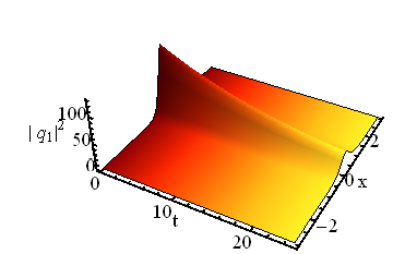
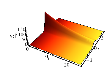
Figure 1: (Color online) Decay of the soliton solution in the time-independent parabolic potential for $\Omega(t)=-0.02$ (or $\gamma(t)=exp[0.02t]$), $\varepsilon_{1}^{(1)}=0.3$, $\alpha_{10}=0.1$, $\beta_{10}=0.3$, $\chi_{1}=0.1$, $\delta_{1}=0.2$.

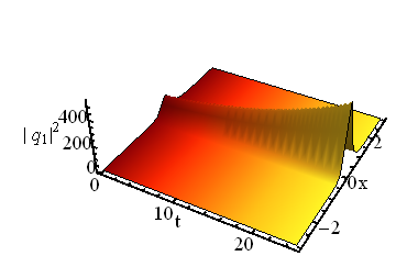
Figure 2: (Color online) Growth of the soliton solution for $\Omega(t)=0.02$ (or $\gamma(t)=exp[-0.02t]$), $\varepsilon_{1}^{(1)}=0.3$, $\alpha_{10}=0.5$, $\beta_{10}=0.5$, $\chi_{1}=0.5$, $\delta_{1}=0.2$.

To stabilize the solitons, we now introduce a time dependence of the parabolic potential, selecting $\Omega(t)$ as shown in Fig. 3. For this case, the density profile of the solution, shown in Fig. 4, indicates that one can sustain the shape of the bright soliton. Accordingly, we call solutions of the type shown in Fig. 4 “persistent bright solitons”.

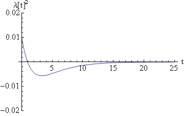
Figure 3: (Color online) Evolution of the strength of the parabolic potential, $\lambda^{2}(t)$ (which may be both positive and negative), given by Eq. (20), for $\gamma(t)=\exp\left[\left(2/3\right)\left(1-e^{-0.3t}\right)\right]$.

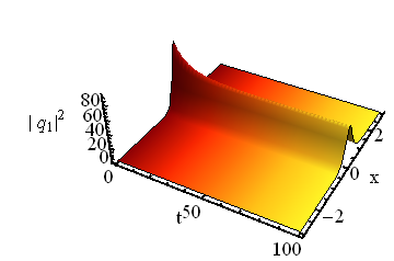
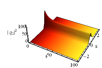
Figure 4: (Color online) A persistent soliton for the same $\gamma(t)$ as in Fig. 3, and $\varepsilon_{1}^{(1)}=0.3$, $\alpha_{10}=0.2$, $\beta_{10}=0.5$, $\chi_{1}=0.5$, $\delta_{1}=0.2$.

4.2 Numerical verification

It is possible to confirm the analytical results by numerical solutions of eq. (2), produced by means of the split-step Crank-Nicolson method. In Fig. 5, we have plotted the persistent bright solitons derived analytically as per eqs. (44) and (45) at $t=10$ and $20$, and the corresponding numerically generated density profiles. Thus, Fig.(5) demonstrates exact matching of the analytical solutions to their numerical counterparts.

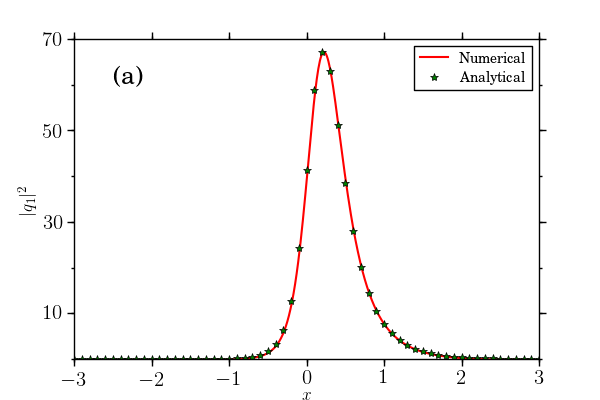
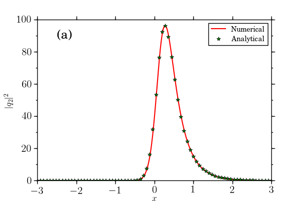
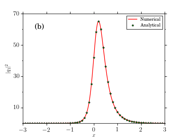
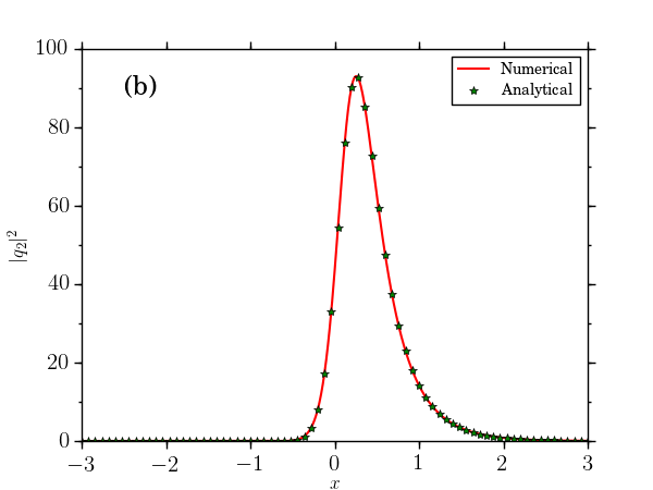
Figure 5: (Color online) Comparison of analytical and numerical solutions for solitons. (a) The upper left panel: the $q_{1}$ component at $t=10$; the upper right panel: $q_{2}$ at $t=10$. (b) The bottom left panel: $q_{1}$ at $t=20$; the bottom right panel: $q_{2}$ at $t=20$. Parameters are the same as in Fig. (4).

Since bright solitons exist due to the special choice of the strength of the parabolic potential as a function of time (see eqs. (18)-(20)), we have also tested the structural stability of the solitons, by suddenly varying the strength of the potential (either increasing or decreasing it by $10\%$), as shown in Figs. (6) and (7). From figs. (6) and (7), we observe that the addition of a small perturbation does not impact the stability of persistent solitons.

Figure 6: (Color online) Density profiles of the fields produced by suddenly increasing the potential’s strength for, $\gamma(t)=exp[(20/3)(1-e^{-0.3t})]$, at (a) $t=10$, (b) $t=20$.

Figure 7: (Color online) The density profiles of the fields obtained while suddenly decreasing the potential’s strength, for $\gamma(t)=exp[(1/15)(1-e^{-0.3t})]$ at (a)$t=10$, (b) $t=20$.

5 Collisional dynamics of bright vector solitons

The gauge-transformation approach can be easily extended to generate multisoliton solutions [27]. In particular,, the two-soliton solution $q_{1,2}^{(2)}$ for the two modes can be expressed as

$$q_{1}^{(2)}=2IA_{1}/B,~{}q_{2}^{(2)}=2IA_{2}/B,$$ (46)

where

$$A_{1} = M_{121}M_{222}\left(\zeta_{2}-\zeta_{1}\right)\left(\zeta_{1}-\zeta_{1}^{\ast}\right)\left(\zeta_{2}-\zeta_{2}^{\ast}\right)+M_{122}M_{221}\left(\zeta_{2}-\zeta_{1}^{\ast}\right)\left(\bar{\zeta_{2}}-\zeta_{1}\right)\left(\zeta_{2}-\zeta_{2}^{\ast}\right)$$

$$+ M_{111}M_{122}\left(\zeta_{2}-\zeta_{1}^{\ast}\right)\left(\zeta_{2}^{\ast}-\zeta_{1}^{\ast}\right)\left(\zeta_{2}-\zeta_{2}^{\ast}\right)+M_{112}M_{121}\left(\zeta_{1}-\zeta_{1}^{\ast}\right)\left(\zeta_{2}^{\ast}-\zeta_{1}\right)\left(\zeta_{2}^{\ast}-\zeta_{1}^{\ast}\right),$$

$$A_{2} = M_{112}M_{211}\left(\zeta_{2}-\zeta_{1}\right)\left(\zeta_{1}-\zeta_{1}^{\ast}\right)\left(\zeta_{2}-\zeta_{2}^{\ast}\right)+M_{111}M_{212}\left(\zeta_{2}-\zeta_{1}^{\ast}\right)\left(\zeta_{2}^{\ast}-\zeta_{1}\right)\left(\zeta_{2}-\zeta_{2}^{\ast}\right)$$

$$+ M_{212}M_{221}\left(\zeta_{2}-\zeta_{1}^{\ast}\right)\left(\zeta_{1}-\zeta_{1}^{\ast}\right)\left(\zeta_{2}-\zeta_{2}^{\ast}\right)+M_{211}M_{222}\left(\zeta_{1}-\zeta_{1}^{\ast}\right)\left(\zeta_{2}^{\ast}-\zeta_{1}\right)\left(\zeta_{2}^{\ast}-\zeta_{1}^{\ast}\right),$$

$$B = \left(M_{122}M_{211}+M_{121}M_{212}\right)\left(\zeta_{1}-\zeta_{1}^{\ast}\right)\left(\zeta_{2}-\zeta_{2}^{\ast}\right)+\left(M_{112}M_{221}+M_{111}M_{222}\right)\left(\zeta_{2}-\zeta_{1}^{\ast}\right)$$

$$\left(\zeta_{2}^{\ast}-\zeta_{1}\right)+\left(M_{111}M_{112}+M_{221}M_{222}\right)\left(\zeta_{2}-\zeta_{1}\right)\left(\zeta_{2}^{\ast}-\zeta_{1}^{\ast}\right),$$

$$M_{11j} = e^{-\theta_{j}}\sqrt{2};\quad M_{12j}=e^{-i\xi_{j}}\varepsilon_{1}^{(j)};\quad M_{13j}=e^{-i\xi_{j}}\varepsilon_{2}^{(j)};$$

$$M_{21j} = e^{i\xi_{j}}\varepsilon_{1}^{\ast(j)};\quad M_{22j}=e^{\theta_{j}}/\sqrt{2};\quad M_{23j}=0;$$

$$M_{31j} = e^{i\xi_{j}}\varepsilon_{2}^{\ast(j)};\quad M_{32j}=0;\quad M_{33j}=e^{\theta_{j}}/\sqrt{2},$$

$$\theta_{j} = 2x\beta_{j}(t)-4\int(\alpha_{j}(t)\beta_{j}(t))dt+2\delta_{j},$$ (47)

$$\xi_{j} = 2x\alpha_{j}(t)-2\int(\alpha_{j}(t)^{2}-\beta_{j}(t)^{2})dt-2\chi_{1},$$ (48)

and $j=1,2$

In Fig. 8, one can observe inelastic collision of persistent solitons. The collisional dynamics predicted by the analytical solution (the top panel in Fig. 8) and its numerical counterpart (the bottom panel in Fig. 8) are identical.

Figure 8: (Color online) Inelastic collision of solitons for the choice $\gamma(t)=\exp\left[\left(2/3\right)\left(1-e^{-0.3t}\right)\right]$., $\alpha_{10}=0.1$, $\alpha_{20}=0.25$, $\beta_{10}=0.3$, $\beta_{20}=0.2$, $\delta_{1}=0.1$, $\delta_{2}=0.2$, $\chi_{1}=0.3$, $\chi_{2}=0.4$, $\varepsilon_{1}^{(1)}=0.85i$, $\varepsilon_{1}^{(2)}=0.5$such that $|\varepsilon_{1}^{(j)}|^{2}+|\varepsilon_{2}^{(j)}|^{2}=1,(j=1,2)$. The top and bottom panels show the analytical solution and its numerical counterpart.

6 Conclusion

The aim of this work is to investigate the dynamics of solitons in the integrable system of coupled NLS equations with “opposite directions” of time in the two subsystems. The system includes the time-dependent nonlinearity coefficient, which must be specifically related to the coefficient in front of the parabolic-potential terms, to secure the integrability. By means of the gauge transformations, we have demonstrated that a special choice of the time dependence of the trap may effectively stabilize bright solitons. We have also observed inelastic collision of persistent solitons for the same choice of trap frequency which is subsequently confirmed by numerical simulations.

7 Acknowledgements

PSV and JBS thank University Grants Commission (UGC) and Department of Science and Technology (DST) of India, respectively, for the financial support. RR wishes to acknowledge the financial assistance received from DST (Ref.No:SR/S2/HEP-26/2012), UGC (Ref.No:F.No 40-420/2011(SR), Department of Atomic Energy -National Board for Higher Mathematics (DAE-NBHM) (Ref.No: NBHM/R.P.16/2014/Fresh dated 22.10.2014) and Council of Scientific and Industrial Research (CSIR) (Ref.No: No.03(1323)/14/EMR-II dated 03.11.2014) dated 4.July.2011) for the financial support in the form Major Research Projects.

References

• [1] Manakov S V. On the theory of two dimensional stationary self-focusing of electromagnetic waves. Zh. Eksp. Teor. Fiz. 1973; 65: 505-516.
• [2] Blow K J, Doran N J, Wood D. Polarization instabilities for solitons in birefringent fibers. Opt. Lett. 1987; 12: 202-204.
• [3] Tratnik M V, Sipe J E. Bound solitary waves in a birefringent optical fiber. Phys. Rev. A 1988; 38: 2011.
• [4] Menyuk C R. Pulse propagation in an elliptically birefringent Kerr medium. IEEE J. Quantum Electronics 1989; 25: 2674-2682.
• [5] De Angelis C, Matera F, Wabnitz S. Soliton instabilities from resonant random mode coupling in birefringent optical fibers. Opt. Lett. 1992; 17: 850-852.
• [6] Sakaguchi H, Malomed B A. Symmetry breaking of solitons in two-component Gross-Pitaevskii equations. Phys. Rev. E 2011; 83: 036608.
• [7] Agrawal G P. Nonlinear Fiber Optics. San Diego: Academic Press; 2001.
• [8] Thalhammer G, Barontini G, De Sarlo L, Catani J, Minardi F, Inguscio M. Double Species Bose-Einstein Condensate with Tunable Interspecies Interactions. Phys. Rev. Lett. 2008; 100: 210402.
• [9] Kutz N J. Mode-locked matter waves in Bose-Einstein condensates. Physica D 2009 ; 238: 1468-1474.
• [10] Middelkamp S, Chang J J, Hamner C, Carretero-González R, Kevrekidis P G, Achilleos V, Frantzeskakis D J, Schmelcher P, Engels P. Dynamics of dark bright solitons in cigar-shaped Bose Einstein condensates. Phys. Lett. A 2011; 375: 642-646.
• [11] Achilleos V, Frantzeskakis D J, Kevrekidis P G, Pelinovsky D E, Matter-Wave Bright Solitons in Spin-Orbit Coupled Bose-Einstein Condensates. Phys. Rev. Lett. 2013;110: 264101.
• [12] Kartashov Y V, Konotop V V, Abdullaev F Kh. Gap Solitons in a Spin-Orbit-Coupled Bose-Einstein Condensate. Phys. Rev. Lett. 2013 ; 111: 060402.
• [13] Xu Y, Zhang Y, Wu B. Bright solitons in spin-orbit-coupled Bose-Einstein condensates. Phys. Rev. A 2013; 87: 013614.
• [14] Salasnich L and Malomed B A. Localized modes in dense repulsive and attractive Bose-Einstein condensates with spin-orbit and Rabi couplings. Phys. Rev. A 2013; 87: 063625.
• [15] Lobanov V E, Kartashov Y V, Konotop V V. Fundamental, Multipole, and Half-Vortex Gap Solitons in Spin-Orbit Coupled Bose-Einstein Condensates. Phys. Rev. Lett. 2014; 112: 180403.
• [16] Sakaguchi H, Li B and Malomed B A. Creation of two-dimensional composite solitons in spin-orbit-coupled self-attractive Bose-Einstein condensates in free space. Phys. Rev. E. 2014; 89: 032920.
• [17] Salasnich L, Cardoso W B and Malomed B A. Localized modes in quasi-two-dimensional Bose-Einstein condensates with spin-orbit and Rabi couplings. Phys. Rev. A 2014; 90: 033629.
• [18] Radha Krishnan R, Lakshmanan M, Hietarinta J. Inelastic collision and switching of coupled bright solitons in optical fibers. Phys. Rev. E. 1997;56: 2213.
• [19] Makhankov V G , Makhaldiani N V, Pashaev O K. On the integrability and isotopic structure of the one-dimensional Hubbard model in the long wave approximation. Phys. Lett. A 1981; 81: 161-164.
• [20] Radha R, Vinayagam P S and Porsezian K, Rotation of the trajectories of bright solitons and realignment of intensity distribution in the coupled nonlinear Schrodinger equation. Phys. Rev. E 2013;88: 032903.
• [21] Saleh M F and Biancalana F. Soliton-radiation trapping in gas-filled photonic crystal fibers. Phys. Rev. A. 2013; 87: 043807.
• [22] Ieda J, Miyakawa T, Wadati M. Exact Analysis of Soliton Dynamics in Spinor Bose-Einstein Condensates. Phys. Rev. Lett. 2004; 93: 194102.
• [23] Feijoo D, Paredes A, Michinel H. Outcoupling vector solitons from a Bose-Einstein condensate with time-dependent interatomic forces. Phys. Rev. A 2013; 87: 063619.
• [24] Veselago V G. The electrodynamics of substances with simultaneously negative values of $\epsilon$ and $\mu$. Sov. Phys. Usp. 1968; 10: 509.
• [25] Lazarides N, Tsironis G P. Coupled nonlinear Schr dinger field equations for electromagnetic wave propagation in nonlinear left-handed materials. Phys. Rev. E. 2005; 71: 036614.
• [26] Park Q H, Shin H J.Painlev analysis of the coupled nonlinear Schr dinger equation for polarized optical waves in an isotropic medium. Phys. Rev. E. 1999; 59: 2373.
• [27] Chau L -L , Shaw J C, Yen H C. An alternative explicit construction of N-soliton solutions in 1+1 dimensions. J. Math. Phys. 1991; 32: 1737.
• [28] Zakharov N E, Schulman E I.To the integrability of the system of two coupled nonlinear Schr dinger equations.Physica D 1982; 4: 270-274.
• [29] Sahadevan R, Tamizhmani K M ,Lakshmanan M. Painleve analysis and integrability of coupled non-linear Schrodinger equations. J. Phys. A. 1986; 19: 1783.
• [30] Kaup D J and Malomed B A. Soliton trapping and daughter waves in the Manakov model. Phys. Rev. A 1993; 48: 599.
• [31] Abdullaev F Kh and Tsoy E N. The evolution of optical beams in self-focusing media. Physica D 2002; 161: 67.
• [32] Zhang X F, Hu X-H, Liu X-X, Liu W M. Vector solitons in two-component Bose-Einstein condensates with tunable interactions and harmonic potential. Phys. Rev. A 2009; 79: 033630.
• [33] Rajendran S, Muruganandam P, Lakshmanan M. Interaction of dark bright solitons in two-component Bose Einstein condensates. J. Phys. B: At. Mol. Opt. Phys. 2009; 42: 145307.
• [34] Ramesh Kumar V, Radha R, Wadati M. Collision of bright vector solitons in two-component Bose Einstein condensates. Phys. Lett. A. 2010; 374: 3685-3694.
• [35] R. Radha, P.S.Vinayagam. Stabilization of matter wave solitons in weakly coupled atomic condensates.Phys. Lett. A. 2012; 376: 944-949.
• [36] Cuevas J, Kevrekidis P G, Malomed B A, Dyke P, Hulet R G.Interactions of solitons with a Gaussian barrier: splitting and recombination in quasi-one-dimensional and three-dimensional settings. New J. Phys.2013; 15: 063006.
• [37] Maimistov A I and Gabitov I R. Nonlinear optical effects in artificial materials. Eur. Phys. J. Special Topics 2007; 147: 265.
• [38] Zhang H Q, Li J, Xu T, Zhang Y X, Hu W, Tian B. Optical soliton solutions for two coupled nonlinear Schr dinger systems via Darboux transformation. Phys. Scr. 2007; 76: 452.
• [39] Atre R, Panigrahi P K, Agarwal G S. Class of solitary wave solutions of the one-dimensional Gross-Pitaevskii equation. Phys. Rev. E 2006; 73: 056611.
• [40] Theocharis G, Rapti Z, Kevrekidis P G, Frantzeskakis D J, Konotop V V. Modulational instability of Gross-Pitaevskii-type equations in 1+1 dimensions. Phys. Rev. A 2003; 67: 063610.
• [41] Wu L, Zhang J-F, Li L. Modulational instability and bright solitary wave solution for Bose Einstein condensates with time-dependent scattering length and harmonic potential. New J. Phys. 2007; 9: 69.
• [42] Ramesh Kumar V, Radha R, Panigrahi P K. Dynamics of Bose-Einstein condensates in a time-dependent trap. Phys. Rev. A. 2008; 77: 023611.
• [43] Sakkaravarti K, Kanna T. Bright solitons in coherently coupled nonlinear Schr dinger equations with alternate signs of nonlinearities.J. Math. Phys. 2013; 54: 013701.
• [44] Radha R, Ramesh Kumar V.Bright matter wave solitons and their collision in Bose Einstein condensates. Phys. Lett A. 2007; 370: 46-50.