DC Proximal Newton for Non-Convex Optimization Problems

Abstract

We introduce a novel algorithm for solving learning problems where both the loss function and the regularizer are non-convex but belong to the class of difference of convex (DC) functions. Our contribution is a new general purpose proximal Newton algorithm that is able to deal with such a situation. The algorithm consists in obtaining a descent direction from an approximation of the loss function and then in performing a line search to ensure sufficient descent. A theoretical analysis is provided showing that the iterates of the proposed algorithm admit as limit points stationary points of the DC objective function. Numerical experiments show that our approach is more efficient than current state of the art for a problem with a convex loss function and a non-convex regularizer. We have also illustrated the benefit of our algorithm in high-dimensional transductive learning problem where both loss function and regularizers are non-convex.

I Introduction

In many real-world application domains such as computational biology, finance or text mining, datasets considered for learning prediction models are routinely large-scale and high-dimensional raising the issue of model complexity control. One way for dealing with such kinds of dataset is to learn sparse models. Hence, a very large amount of recent works in machine learning, statistics and signal processing have addressed optimization problems related to sparsity issues.

One of the most popular algorithm for achieving sparse models is the Lasso algorithm [1] also known as the Basis pursuit algorithm [2] in the signal processing community. This algorithm actually applies $\ell_{1}$-norm regularization to the learning model. The choice of the $\ell_{1}$ norm comes from its appealing properties which are convexity, continuity and its ability to produce sparse or even the sparsest model in some cases owing to its non-differentiability at zero [3, 4]. Since these seminal works, several efforts have been devoted to the development of efficient algorithms for solving learning problems that consider sparsity-inducing regularizers [5, 6, 7, 8]. However, $\ell_{1}$ regularizer presents some drawbacks such as its inability, in certain situations to retrieve the true relevant variables of a model [9, 10]. Since the $\ell_{1}$-norm regularizer is a continuous and convex surrogate of the $\ell_{0}$ pseudo-norm, other kinds of regularizer which abandon the convexity property, have been analyzed by several authors and they have been proved to achieve better statistical property. Common non-convex and non-differentiable regularizers are the SCAD regularizer [10], the $\ell_{p}$ regularizer [11], the capped-$\ell_{1}$ and the log penalty [12]. These regularizers have been frequently used for feature selections or for obtaining sparse models [13, 14, 12].

While being statistically appealing, the use of these non-convex and non-smooth regularizers poses some challenging optimization problems. In this work, we propose a novel efficient non-convex proximal Newton algorithm. Indeed, one of the most frequently used algorithms for solving $\ell_{1}$-norm regularized problem is the proximal gradient algorithm [15]. Recently, proximal Newton-type methods have been introduced for solving composite optimization problems involving the sum of a smooth and convex twice differentiable function and a non-smooth convex function (typically the regularizer)[16, 17]. These proximal Newton algorithms have been shown to be substantially faster than their proximal gradient counterpart. Our objective is thus to go beyond the state-of-the-art by proposing an efficient proximal Newton algorithm that is able to handle machine learning problems where the loss function is smooth and possibly non-convex and the regularizer is non-smooth and non-convex.

Based on this, we propose an effficient general proximal Newton method for optimizing a composite objective function $f(\mathbf{x})+h(\mathbf{x})$ where both functions $f$ and $h$ can be non-convex and belong to a large class of functions that can be decomposed as the difference of two convex functions (DC functions) [18, 19, 20]. In addition, we also allow $h(\mathbf{x})$ to be non-smooth, which is necessary for sparsity promoting regularization. The proposed algorithm has a wide range of applicability that goes far beyond the handling of non-convex regularizers. Indeed, our global framework can genuinely deal with non-convex loss functions that usually appear in learning problems. To make concrete the DC Newton proximal approach, we illustrate the relevance and the effectiveness of the novel algorithm by considering a problem of sparse transductive logistic regression in which the regularizer as well as the loss related to the unlabeled examples are non-convex. As far as our knowledge goes, this is the first work that introduces such a model and proposes an algorithm for solving the related optimization problem. In addition to this specific problem, many non-convex optimization problems involving non-convex loss functions and non-convex and non-differentiable regularizers arise in machine learning e.g dictionary learning [21, 22] or matrix factorization [23] problems. In addition, several works have recently shown that non-convex loss functions such as the Ramp loss which is a DC function, lead to classifiers more robust to outliers [24, 25]. We thus believe that the proposed framework is of general interest in machine learning optimization problems involving this kind of losses and regularizers.

The algorithm we propose consists in two steps: first it seeks a search direction and then it looks for a step-size in that direction that minimizes the objective value. The originality and main novelty we brought in this work is that the search direction is obtained by solving a subproblem which involves both an approximation of the smooth loss function and the DC regularizer. Note that while our algorithm for non-convex objective function is rather similar to the convex proximal Newton method, non-convexity and non-differentiability raise some technical issues when analysing the properties of the algorithm. Nonetheless, we prove several properties related to the search direction and provide convergence analysis of the algorithm to a stationary point of the related optimization problem. These properties are obtained as non-trivial extension of the convex proximal Newton case. Experimental studies show the benefit of the algorithm in terms of running time while preserving or improving generalization performance compared to existing non-convex approaches.

The paper is organized as follows. Section II introduces the general optimization problem we want to address as well as the proposed DC proximal Newton optimization scheme. Details on the implementation and discussion concerning related works are also provided. In Section III, an analysis of the properties of the algorithm is given. Numerical experiments on simulated and real-world data comparing our approach to the existing methods are depicted in Section IV, while Section V concludes the paper.

II DC proximal Newton algorithm

We are interested in solving the following optimization problem

$$\min_{\mathbf{x}\in\mathbb{R}^{d}}\,F(\mathbf{x}):=f(\mathbf{x})+h(\mathbf{x})$$ (1)

with the following assumptions concerning the functions $f$ and $h$. $f$ is supposed to be twice differentiable, lower bounded on $\mathbb{R}^{d}$ and we suppose that there exists two convex functions $f_{1}$ and $f_{2}$ such that $f$ can be written as a difference of convex (DC) functions $f(\mathbf{x})=f_{1}(\mathbf{x})-f_{2}(\mathbf{x})$. We also assume that $f_{1}$ verifies the $L$-Lipschitz gradient property

$$\|\nabla f_{1}(\mathbf{x})-\nabla f_{1}(\mathbf{y})\|\leq L\|\mathbf{x}-\mathbf{y}\|\quad\forall\mathbf{x},\mathbf{y}\in\text{dom}f_{1}.$$

The DC assumption on $f$ is not very restrictive since any differentiable function $f(\cdot)$ with a bounded Hessian matrix can be expressed as a difference of convex function [26].

The function $h$ is supposed to be a lower-bounded, proper, lower semi-continuous and its restriction to its domain is continuous. We suppose that $h$ that can also be expressed as

$$h(\mathbf{x})=h_{1}(\mathbf{x})-h_{2}(\mathbf{x})$$ (2)

where $h_{1}$ and $h_{2}$ are both convex functions. As discussed in the introduction, we focus our interest in situations where $h$ is non-convex and non-differentiable. As such $h_{1}$ and $h_{2}$ are also expected to be non-differentiable. A large class of non-convex sparsity-inducing regularizers can be expressed as a DC function as discussed in [14]. This includes the classical SCAD regularizer, the $\ell_{p}$ regularizer, the capped-$\ell_{1}$ and the log penalty as above-mentioned.

Note that those assumptions on $f$ and $h$ cover a broad class of optimization problems. Proposed approach can be applied for sparse linear model estimation as illustrated in in Section IV. But more general learning problems such as those using overlapping nonconvex $\ell_{p}-\ell_{1}$ (with $p<1$) group-lasso as used in [27] can also be considered. Our framework also encompasses those of structured sparse dictionary learning or matrix factorization [28, 22], sparse and low-rank matrix estimation [29, 30], or maximum likekihood estimation of graphical models [31], when the $\ell_{1}$ sparsity-inducing regularizer is replaced for instance by a more aggressive regularizer like the log penalty or the SCAD regularizer.

II-A Optimization scheme

For solving Problem (1) which is a difference of convex functions optimization problem, we propose a novel iterative algorithm which first looks for a search direction $\Delta\mathbf{x}$ and then updates the current solution. Formally, the algorithm is based on the iteration

$$\mathbf{x}_{k+1}=\mathbf{x}_{k}+t_{k}\Delta\mathbf{x}_{k}$$

where $t_{k}$ and $\Delta\mathbf{x}_{k}$ are respectively a step size and the search direction. Similarly to the works of Lee et al. [16], the search direction is computed by minimizing a local approximation of the composite function $F(\mathbf{x})$. However, we show that by using a simple approximation on $f_{1}$, $f_{2}$ and $h_{2}$, we are able to handle the non-convexity of $F(\mathbf{x})$, resulting in an algorithm which is wrapped around a specific proximal Newton iteration.

For dealing with the non-convex situation, we define the search direction as the solution of the following problem

$$\Delta\mathbf{x}_{k}=\operatorname*{arg\,min}_{\Delta\mathbf{x}}\tilde{f}(\mathbf{x}_{k}+\Delta\mathbf{x})+\tilde{h}(\mathbf{x}_{k}+\Delta\mathbf{x})$$ (3)

where $\tilde{f}$ and $\tilde{h}$ are the following approximations of respectively $f$ and $h$ at $\mathbf{x}_{k}$. We define $\tilde{f}(\mathbf{x})$ as

$$\tilde{f}(\mathbf{x}) = f_{1}(\mathbf{x}_{k})+\nabla f_{1}(\mathbf{x}_{k})^{\top}(\mathbf{x}-\mathbf{x}_{k})$$

$$+\leavevmode\nobreak\ \frac{1}{2}(\mathbf{x}-\mathbf{x}_{k})^{\top}\mathbf{H}_{k}(\mathbf{x}-\mathbf{x}_{k})$$

$$-\leavevmode\nobreak\ f_{2}(\mathbf{x}_{k})-\mathbf{z}_{f_{2}}^{\top}(\mathbf{x}-\mathbf{x}_{k})$$

where $\mathbf{z}_{f_{2}}={{\color[rgb]{0,0,0}\nabla}}f_{2}(\mathbf{x}_{k})$ and $\mathbf{H}_{k}$ is any positive definite approximation of the Hessian matrix of $f_{1}$ at current iterate. We also consider

$$\tilde{h}(\mathbf{x})=h_{1}(\mathbf{x})-h_{2}(\mathbf{x}_{k})-\mathbf{z}_{{\color[rgb]{0,0,0}h_{2}}}^{\top}(\mathbf{x}-\mathbf{x}_{k})$$ (5)

where $\mathbf{z}_{{\color[rgb]{0,0,0}h_{2}}}\in\partial h_{2}(\mathbf{x}_{k})$, with the latter being the sub-differential of $h_{2}$ at $\mathbf{x}_{k}$.

Note that the first three summands in Equation (II-A) form a quadratic approximation of $f_{1}(\mathbf{x})$ whereas the terms in the third line of Equation (II-A) is a linear approximation of $f_{2}(\mathbf{x})$. In the same spirit, $\tilde{h}$ is actually a majorizing function of $h$ since we have linearized the convex function $h_{2}$ and $h$ is a difference of convex functions.

We are now in position to provide the proximal expression of the search direction. Indeed, Problem (3) can be rewritten as

$$\operatorname*{arg\,min}_{\Delta\mathbf{x}}\frac{1}{2}\Delta\mathbf{x}^{\top}\mathbf{H}_{k}\Delta\mathbf{x}+h_{1}(\mathbf{x}_{k}+\Delta\mathbf{x})+{\mathbf{v}_{k}}^{\top}\Delta\mathbf{x}$$ (6)

with $\mathbf{v}_{k}=\nabla f_{{\color[rgb]{0,0,0}1}}(\mathbf{x}_{k})-\mathbf{z}_{f_{2}}-\mathbf{z}_{h_{2}}$. After some algebras given in the appendix and involving optimality conditions of a proximal Newton operator, we can show that

$$\Delta\mathbf{x}_{k}={\textbf{prox}}_{h_{1}}^{\mathbf{H}_{k}}(\mathbf{x}_{k}-\mathbf{H}_{k}^{-1}\mathbf{v}_{k})-\mathbf{x}_{k}$$ (7)

with by definition [15, 16]

$${\textbf{prox}}_{h_{1}}^{\mathbf{H}}(\mathbf{x})=\arg\min_{\mathbf{y}}\frac{1}{2}\|\mathbf{x}-\mathbf{y}\|_{\mathbf{H}}^{2}+h_{1}(\mathbf{y})$$

where $\|\mathbf{x}\|_{\mathbf{H}}^{2}=\mathbf{x}^{\top}\mathbf{H}\mathbf{x}$ is the quadratic norm with metric $\mathbf{H}$. Interestingly, we note that the non-convexity of the initial problem is taken into account only through the proximal Newton operator and its impact on the algorithm, compared to the convex case, is minor since it only modifies the argument of the operator through $\mathbf{v}_{k}$.

Once the search direction is computed, the step size $t_{k}$ is backtracked starting from $t_{k}=1$. Algorithm 1 summarizes the main steps of the optimization scheme. Some implementation issues are discussed hereafter while the next section focuses on the convergence analysis.

Algorithm 1 DC proximal Newton algorithm

1:  Initialize $\mathbf{x}_{0}\in dom{{\color[rgb]{0,0,0}F}}$

2:  $k=0$

3:  repeat

4:     compute $\mathbf{z}_{h_{2}}\in\partial h_{2}(\mathbf{x}_{k})$ and $\mathbf{z}_{f_{2}}=\nabla f_{2}(\mathbf{x}_{k})$

5:     update $\mathbf{H}_{k}$ (exactly or using a quasi-Newton approach)

6:     $\mathbf{v}_{k}\leftarrow\nabla f_{1}(\mathbf{x}_{k})-\mathbf{z}_{f_{2}}-\mathbf{z}_{h_{2}}$

7:     $\Delta\mathbf{x}_{k}\leftarrow{\textbf{prox}}_{h_{1}}^{\mathbf{H}_{k}}(\mathbf{x}_{k}-\mathbf{H}_{k}^{-1}\mathbf{v}_{k})-\mathbf{x}_{k}$

8:     compute the stepsize $t_{k}$ through backtracking starting from $t_{k}=1$

9:     $\mathbf{x}_{k+1}=\mathbf{x}_{k}+t_{k}\Delta{\mathbf{x}_{k}}$

10:     $k\leftarrow k+1$

11:  until convergence criterion is met

II-B Implementation’s tricks of the trade

The main difficulty and computational burden of our DC proximal Newton algorithm resides in the computation of the search direction $\Delta\mathbf{x}_{k}$. Indeed, the latter needs the computation of the proximal operator ${\textbf{prox}}_{h_{1}}^{\mathbf{H}_{k}}(\mathbf{x}_{k}-\mathbf{H}_{k}^{-1}\mathbf{v}_{k})$ which is equal to

$$\operatorname*{arg\,min}_{\mathbf{y}}\underbrace{\frac{1}{2}\mathbf{y}^{\top}\mathbf{H}_{k}\mathbf{y}{\color[rgb]{0,0,0}+}\mathbf{y}^{\top}(\mathbf{v}_{k}-\mathbf{H}_{k}\mathbf{x}_{k})}_{g(\mathbf{y})}+h_{1}(\mathbf{y})$$ (8)

We can note that Equation 8 represents a quadratic problem penalized by $h_{1}$. If $h_{1}(\mathbf{y})$ is a term which proximal operator can be cheaply computed then, one can consider proximal gradient algorithm or any other efficient algorithms for its resolution [6, 32].

In our case, we have considered a forward-backward (FB) algorithm [15] initialized with the previous value of the optimal $\mathbf{y}$. Note that in order to have a convergence guarantee, the FB algorithm needs a stepsize smaller than $\frac{2}{L}$ where $L$ is the Lipschitz gradient of the quadratic function. Again computing $L$ can be expensive and in order to increase the computational efficiency of the global algorithm, we have chosen a strategy that roughly estimates $L$ according to the equation

$$\frac{\|\nabla g(\mathbf{y})-\nabla g(\mathbf{y}^{\prime}{{\color[rgb]{0,0,0})}}\|_{2}}{\|\mathbf{y}-\mathbf{y}^{\prime}\|_{2}}$$

In practice, we have found this heuristic to be slightly more efficient than an approach which computes the largest eigenvalue of $\mathbf{H}_{k}$ by means of a power method [33]. Note that a L-BFGS approximation scheme has been used in the numerical experiments for updating the matrix $\mathbf{H}_{k}$ and its inverse.

While the convergence analysis we provide in the next section supposes that the proximal operator is computed exactly, in practice it is more efficient to approximately solve the search direction problem, at least for the early iterations. Following this idea, we have considered an adaptive stopping criterion for the proximal operator subproblem.

II-C Related works

In the last few years, a large amount of works have been devoted to the resolution of composite optimization problem of the form given in Equation (1). We review the ones that are most similar to ours and summarize the most important ones in Table I.

Proximal Newton algorithms have recently been proposed by [16] and [17] for solving Equation (1) when both functions $f(\mathbf{x})$ and $h(\mathbf{x})$ are convex. While the algorithm we propose is similar to the one of [16], our work is strictly more general in the sense that we abandon the convexity hypothesis on both functions. Indeed, our algorithm can handle both convex and non-convex cases and boils down to the algorithm of [16] in the convex case. Hence, the main contribution that differentiates our work to the work of Lee et al. [16] relies on the extension of the algorithm to the non-convex case and the theoretical analysis of the resulting algorithm.

Table I: Summary of related approaches according to how $f(\mathbf{x})$ and $h(\mathbf{x})$ are decomposed in $f_{1}-f_{2}$ and $h_{1}-h_{2}$. cvx and ncvx respectively stands for convex and non-convex. $-$ denotes that the method that does not handle DC functions. The metric column denotes the form of the metric used in the quadratic approximation.

	f($\mathbf{x}$)		h($\mathbf{x}$)		metric
Approach	$f_{1}$	$f_{2}$	$h_{1}$	$h_{2}$	$\mathbf{H}$
proximal gradient [15]	cvx	-	cvx	-	$\frac{L}{2}$$\mathbf{I}$
proximal Newton [16]	cvx	-	cvx	-	$\mathbf{H}_{k}$
GIST [34]	ncvx	-	cvx	cvx	$\frac{L}{2}$$\mathbf{I}$
SQP [35]	cvx	cvx	cvx	cvx	$\frac{L}{2}$$\mathbf{I}$
our approach	cvx	cvx	cvx	cvx	$\mathbf{H}_{k}$

Following the interest on sparsity-inducing regularizers, there has been a renewal of curiosity around non-convex optimization problems [12, 13]. Indeed, most statistically relevant sparsity-inducing regularizers are non-convex [36]. Hence, several researchers have proposed novel algorithms for handling these isssues.

We point out that linearizing the concave part in a DC program is a crucial idea of DC programming and DCA that were introduced by Pham Dinh Tao in the early eighties and have been extensively developed since then [18, 37, 19]. In this work, we have used this same idea in a proximal Newton framework. However, our algorithm is fairly different from the DCA [19] as we consider a single descent step at each iteration, as opposed to the DCA which needs a full optimization of a minimization problem at each iteration. This DCA algorithm has as special case, the convex concave procedure (CCCP) introduced by Yuille et al. [26] and used for instance by Collobert et. al [38] in a machine learning context.

This idea of linearizing the (possibly) non-convex part of Problem (1) for obtaining a search direction can also be found in Mine and Fukushima [39]. However, in their case, the function to be linearized is supposed to be smooth. The advantage of using a DC program, as in our case, is that the linearization trick can also be extended to non-smooth function.

The works that are mostly related to ours are those proposed by [34] and [35]. Interestingly, Gong et al. [34] introduced a generalized iterative shrinkage algorithm (GIST) that can handle optimization problems with DC regularizers for which proximal operators can be easily computed. Instead, Lu [35] solves the same optimization problem in a different way. As the non-convex regularizers are supposed to be DC, he proposes to solve a sequence of convex programs which at each iteration minimizes

$$\tilde{f}(\mathbf{x})+h_{1}(\mathbf{x})-h_{2}(\mathbf{x}_{k})-\mathbf{z}_{h_{2}}^{\top}(\mathbf{x}-\mathbf{x}_{k})$$

with

$$\tilde{f}(\mathbf{x})=f_{1}(\mathbf{x}_{k})+\nabla f_{1}(\mathbf{x}_{k})^{\top}(\mathbf{x}-\mathbf{x}_{k})+\frac{{L}}{2}\|\mathbf{x}-\mathbf{x}_{k}\|^{2}$$

Note that our framework subsumes the one of Lu [35] (when considering unconstrained optimization problem). Indeed, we take into account a variable metric $\mathbf{H}_{k}$ into the proximal term. Thus, the approach of Lu can be deemed a particular case of our method where $\mathbf{H}_{k}={L\,}\mathbf{I}$ at all iterations of the algorithm. Hence, when $f(\mathbf{x})$ is convex, we expect more efficiency compared to the algorithms of [34] and [35] owing to the variable metric $\mathbf{H}_{k}$ that has been introduced.

Very recently, Chouzenoux et al. [40] introduced a proximal Newton-like algorithm for minimizing the sum of a twice differentiable function and a convex function. They essentially consider that the regularization term is convex while the loss function may be non-convex. Their work can thus be seen as an extension of the one of [41] to the variable metric $\mathbf{H}_{k}$ case. Compared to our work, [40] do not impose a DC condition on the function $f(\mathbf{x})$. However, at each iteration, they need a quadratic surrogate function at a point $\mathbf{x}_{k}$ that majorizes $f(\mathbf{x})$. In our case, only the non-convex part is majorized through a simple linearization.

III Analysis

Our objective in this section is to show that our algorithm is well-behaved and to prove at which extents the iterates $\{\mathbf{x}_{k}\}$ converge to a stationary point of Problem (1). We first characterize stationary points of Problem 1 with respects to $\Delta\mathbf{x}$ and then show that all limit points of the sequence $\{\mathbf{x}_{k}\}$ generated by our algorithm are stationary points.

Throughout this work, we use the following definition of a stationary point.

Definition 1

A point $\mathbf{x}^{\star}$ is said to be a stationary point of Problem (1) if

$$0\in\nabla f_{1}(\mathbf{x}^{\star})-\nabla f_{2}(\mathbf{x}^{\star})+\partial h_{1}(\mathbf{x}^{\star})-\partial h_{2}(\mathbf{x}^{\star})$$

Note that being a stationary point, as defined above, is a necessary condition for a point $\mathbf{x}^{\star}$ to be a local minimizer of Problem (1).

According to the above definition, we have the following lemma :

Lemma 1

Suppose $\mathbf{H}_{\star}\succ 0$, $\mathbf{x}^{\star}$ is a stationary point of Problem (1) if and only if $\Delta\mathbf{x}^{\star}=0$ with

$$\Delta\mathbf{x}^{\star}=\operatorname*{arg\,min}_{\mathbf{d}}(\mathbf{v}^{\star})^{\top}\mathbf{d}+\frac{1}{2}\mathbf{d}^{\top}\mathbf{H}_{\star}\mathbf{d}+h_{1}(\mathbf{x}^{\star}+\mathbf{d})$$ (9)

and $\mathbf{v}^{\star}=\nabla f_{1}(\mathbf{x}^{\star})-\mathbf{z}_{f_{2}}^{\star}-\mathbf{z}_{h_{2}}^{\star}$, $\mathbf{z}_{f_{2}}^{\star}=\nabla f_{2}(\mathbf{x}^{\star})$ and $\mathbf{z}_{h_{2}}^{\star}\in\partial h_{2}(\mathbf{x}^{\star})$.

Proof : Let us start by characterizing the solution $\Delta\mathbf{x}^{\star}$. By definition, we have $\Delta\mathbf{x}^{\star}+\mathbf{x}^{\star}={\textbf{prox}}_{h_{1}}^{\mathbf{H}_{\star}}(\mathbf{x}^{\star}-\mathbf{H}_{\star}^{-1}\mathbf{v}^{\star})$ and thus according to the optimality condition of the proximal operator, the following equation holds

$$\mathbf{H}_{\star}(\mathbf{x}^{\star}-\mathbf{H}_{\star}^{-1}\mathbf{v}^{\star}-\Delta\mathbf{x}^{\star}-\mathbf{x}^{\star})\in\partial h_{1}(\Delta\mathbf{x}^{\star}+\mathbf{x}^{\star})$$

which after rearrangement is equivalent to

$$\mathbf{z}_{h_{2}}^{\star}-\mathbf{H}_{\star}\Delta\mathbf{x}^{\star}\in{{\color[rgb]{0,0,0}\nabla f(\mathbf{x}^{\star})}}+\partial h_{1}(\Delta\mathbf{x}^{\star}+\mathbf{x}^{\star})$$ (10)

with $\nabla f(\mathbf{x}^{\star})=\nabla f_{1}(\mathbf{x}^{\star})-\nabla f_{2}(\mathbf{x}^{\star})$. This also means that there exists a $\mathbf{z}_{h_{1}\Delta}^{\star}\in\partial h_{1}(\Delta\mathbf{x}^{\star}+\mathbf{x}^{\star})$ so that

$$\mathbf{z}_{h_{2}}^{\star}-\mathbf{H}_{\star}\Delta\mathbf{x}^{\star}-{{\color[rgb]{0,0,0}\nabla f(\mathbf{x}^{\star})}}-\mathbf{z}_{h_{1}\Delta}^{\star}=\mathbf{0}$$ (11)

Remember that by hypothesis, since $\mathbf{x}^{\star}$ is a stationary point of Problem (1), we have

$$\mathbf{0}\in{{\color[rgb]{0,0,0}\nabla f(\mathbf{x}^{\star})}}+\partial h_{1}(\mathbf{x}^{\star})-\partial h_{2}(\mathbf{x}^{\star})$$

We now prove that if $\mathbf{x}^{\star}$ is a stationary point of Problem (1) then $\Delta\mathbf{x}{{}^{*}}=\mathbf{0}$ by showing the contrapositive. Suppose that $\Delta\mathbf{x}^{\star}\neq\mathbf{0}$. $\Delta\mathbf{x}^{\star}$ is a vector that satisfies the optimality condition (10) and it is the unique one according to properties of the proximal operator. This means that the vector $\mathbf{0}$ is not optimal for the problem (9) and thus it does not exist a vector $\mathbf{z}_{h_{1}\mathbf{0}}^{\star}\in\partial h_{1}(\mathbf{d}+\mathbf{x}^{\star})$ so that

$$\mathbf{z}_{h_{2}}^{\star}-\mathbf{H}_{\star}\mathbf{d}-{{\color[rgb]{0,0,0}\nabla f(\mathbf{x}^{\star})}}-\mathbf{z}_{h_{1}\mathbf{0}}^{\star}=\mathbf{0}$$ (12)

with $\mathbf{d}=\mathbf{0}$. Note that this equation is valid for any $\mathbf{z}_{h_{2}}^{\star}$ chosen in the set $\partial h_{2}(\mathbf{x}^{\star})$ and the above equation also translates in $\not\exists,\mathbf{z}_{h_{1}\mathbf{0}}^{\star}\in\partial h_{1}(\mathbf{x}^{\star})$ so that $\nabla f(\mathbf{x}^{\star})+\mathbf{z}_{h_{1}\mathbf{0}}^{\star}-\mathbf{z}_{h_{2}}^{\star}=\mathbf{0}$, which proves that $\mathbf{x}^{\star}$ is not a stationary point of problem (1).

Suppose now that $\Delta\mathbf{x}^{\star}=\mathbf{0}$, then according to the definition of $\Delta\mathbf{x}^{\star}$ and the resulting condition (10), it is straightforward to note that $\mathbf{x}^{\star}$ satisfies the definition of a stationary point. $\square$

Now, we proceed by showing that at each iteration, the search direction $\Delta\mathbf{x}_{k}$ satisfies a property which implies that for a sufficiently small step size $t_{k}$, the search direction is a descent direction.

Lemma 2

For $\mathbf{x}_{k}$ in the domain of $f$ and supposing that $\mathbf{H}_{k}\succ 0$ then $\Delta\mathbf{x}_{k}$ is so that

$$F(\mathbf{x}_{k+1}) \leq F(\mathbf{x}_{k})+t_{k}\Big{(}\mathbf{v}_{k}^{\top}\Delta\mathbf{x}_{k}+h_{1}(\Delta\mathbf{x}_{k}+\mathbf{x}_{k})-h_{1}(\mathbf{x}_{k})\Big{)}$$

$$\leavevmode\nobreak\ +O(t_{{\color[rgb]{0,0,0}k}}^{2})$$

and

$$F(\mathbf{x}_{k+1})-F(\mathbf{x}_{k})\leq-t_{k}\Delta\mathbf{x}_{k}^{\top}\mathbf{H}_{k}\Delta\mathbf{x}_{k}+O(t_{k}^{2})$$ (13)

with $\mathbf{v}_{k}=\nabla f_{1}(\mathbf{x}_{k})-\mathbf{z}_{f_{2}}-\mathbf{z}_{h_{2}}$.

Proof: For a sake of clarity, we have dropped the index $k$ and used the following notation. $\mathbf{x}:=\mathbf{x}_{k}$, $\Delta\mathbf{x}:=\Delta\mathbf{x}_{k}$, $\mathbf{x}_{+}:=\mathbf{x}_{k}+t_{k}\Delta\mathbf{x}_{k}$. By definition, we have

$$F(\mathbf{x}_{+})-F(\mathbf{x}) =f_{1}(\mathbf{x}_{+})-f_{{\color[rgb]{0,0,0}1}}(\mathbf{x})-f_{2}(\mathbf{x}_{+})+f_{2}(\mathbf{x})$$

$$+h_{1}(\mathbf{x}_{+})-h_{1}(\mathbf{x})-h_{2}(\mathbf{x}_{+})+h_{2}(\mathbf{x}){\color[rgb]{0,0,0}.}$$

Then by convexity of $f_{2}$, $h_{2}$, $h_{1}$ and for $t\in[0,1]$, we respectively have

$$-\mathbf{z}_{f_{2}}^{\top}(\mathbf{x}_{+}-\mathbf{x})\geq f_{2}(\mathbf{x})-f_{2}(\mathbf{x}_{+}),$$

$$-\mathbf{z}_{h_{2}}^{\top}(\mathbf{x}_{+}-\mathbf{x})\geq h_{2}(\mathbf{x})-h_{2}(\mathbf{x}_{+})$$

and

$$h_{1}(\mathbf{x}+t\Delta\mathbf{x})\leq th_{1}(\mathbf{x}+\Delta\mathbf{x})+(1-t)h_{1}(\mathbf{x})$$

Plugging these inequalities in the definition of $F(\mathbf{x}_{+})-F(\mathbf{x})$ gives :

$$F(\mathbf{x}_{+})-F(\mathbf{x}) \leq f_{1}(\mathbf{x}_{+})-f_{1}(\mathbf{x})+(1-t)h_{1}(\mathbf{x})$$ (14)

$$\;\;+th_{1}(\mathbf{x}+\Delta\mathbf{x})$$

$$\;\;{-t(\mathbf{z}_{f_{2}}+\mathbf{z}_{h_{2}})^{\top}\Delta\mathbf{x}-h_{1}(\mathbf{x})}$$

$$\leq t\nabla f_{1}(\mathbf{x})^{\top}\Delta\mathbf{x}+th_{1}(\mathbf{x}+\Delta\mathbf{x})$$

$$\;\;-th_{1}(\mathbf{x})-t(\mathbf{z}_{f_{2}}+\mathbf{z}_{h_{2}})^{\top}\Delta\mathbf{x}+O(t^{2})$$

which proves the first inequality of the lemma.

For showing the descent property, we demonstrate that the following inequality holds

$$\underbrace{\mathbf{v}^{\top}\Delta\mathbf{x}+h_{1}(\mathbf{x}+\Delta\mathbf{x})-h_{1}(\mathbf{x})}_{D}\leq-\Delta\mathbf{x}^{\top}\mathbf{H}\Delta\mathbf{x}$$ (15)

Since $\Delta\mathbf{x}$ is the minimizer of Problem (6), the following equation holds for $t\Delta\mathbf{x}$ and $t\in[0,1]$:

$$\frac{1}{2}\Delta\mathbf{x}^{\top}\mathbf{H}\Delta\mathbf{x}+h_{1}(\mathbf{x}+\Delta\mathbf{x})+{\mathbf{v}}^{\top}\Delta\mathbf{x}$$ (16)

$$\leq\frac{t^{2}}{2}\Delta\mathbf{x}^{\top}\mathbf{H}\Delta\mathbf{x}+h_{1}(\mathbf{x}+t\Delta\mathbf{x})+t{\mathbf{v}}^{\top}\Delta\mathbf{x}$$

$$\leq\frac{t^{2}}{2}\Delta\mathbf{x}^{\top}\mathbf{H}\Delta\mathbf{x}+(1-t)h_{1}(\mathbf{x})+th_{1}(\mathbf{x}+\Delta\mathbf{x})$$

$$\quad{+t{\mathbf{v}}^{\top}\Delta\mathbf{x}}$$

After rearrangement we have the inequality

$$\mathbf{v}^{\top}\Delta\mathbf{x}+h_{1}(\mathbf{x}+\Delta\mathbf{x})-h_{1}(\mathbf{x})\leq-\frac{1}{2}(1+t)\Delta\mathbf{x}^{\top}\mathbf{H}\Delta\mathbf{x}$$

which is valid for all $t\in[0,1]$ and in particular for $t=1$ which concludes the proof of inequality. By plugging this result into inequality (14), the descent property holds. $\square$

Note that the descent property is supposed to hold for sufficiently small step size. In our algorithm, this stepsize $t_{k}$ is selected by backtracking so that the following sufficient descent condition holds

$$F(\mathbf{x}_{k+1})-F(\mathbf{x}_{k})\leq\alpha t_{k}D_{k}$$ (17)

with $\alpha\in(0,1/2)$. The next lemma shows that if the function $f_{1}$ is sufficiently smooth, then there always exists a step size so that the above sufficient descent condition holds.

Lemma 3

For $\mathbf{x}$ in the domain of $f$ and assuming that $\mathbf{H}_{k}\succeq m\mathbf{I}$ with $m>0$ and $\nabla f_{1}$ is Lipschitz with constant $L$ then the sufficient descent condition in Equation (17) holds for all $t_{k}$ so that

$$t_{k}\leq\min\left(1,2m\frac{1-\alpha}{L}\right)$$

Proof : This technical proof has been post-poned to the appendix. $\square$

According to the above lemma, we can suppose that if some mild conditions on $f_{1}$ are satisfied (smoothness and bounded curvature) then, we can expect our DC algorithm to behave properly. This intuition is formalized in the following property.

Proposition 1

Suppose $f_{1}$ has a gradient which is Lipschitz continuous with constant $L$ and that $\mathbf{H}_{k}\succeq m\mathbf{I}$ for all $k$ and $m>0$, then all the limit points of the sequence $\{\mathbf{x}_{k}\}$ are stationary points.

Proof : Let $\mathbf{x}^{\star}$ be a limit point of the sequence $\{\mathbf{x}_{k}\}$ then, there exists a subsequence $\mathcal{K}$ so that

$$\lim_{k\rightarrow\mathcal{K}}\mathbf{x}_{k}=\mathbf{x}^{\star}$$

At each iteration the step size $t_{k}$ has been chosen so as to satisfy the sufficient descent condition given in Equation (17). According to the above Lemma 3, the step size $t_{k}$ is chosen so as to ensure a sufficient descent and we know that such a step size always exists and it is always non-zero. Hence the sequence $\{F(\mathbf{x}_{k})\}$ is a strictly decreasing sequence. As $F$ is lower bounded, the sequence $\{F(\mathbf{x}_{k})\}$ converges to some limit. Thus, we have

$$\lim_{k\rightarrow\infty}F(\mathbf{x}_{k})=\lim_{k\rightarrow\mathcal{K}}F(\mathbf{x}_{k})=F(\mathbf{x}^{\star})$$

as $F(\cdot)$ is continuous. Thus, we also have

$$\lim_{k\rightarrow\mathcal{K}}F(\mathbf{x}_{k+1})-F(\mathbf{x}_{k})=0$$

Now because each term $F(\mathbf{x}_{k+1})-F(\mathbf{x}_{k}{\color[rgb]{0,0,0})}$ is negative, we can also deduce from Equations (15) and (17) and the limit of $F(\mathbf{x}_{k+1})-F(\mathbf{x}_{k})$ that

$$\lim_{k\rightarrow\mathcal{K}}\mathbf{v}_{k}^{\top}\Delta\mathbf{x}_{k}+h_{1}(\mathbf{x}_{k}+\Delta\mathbf{x}_{k})-h_{1}(\mathbf{x}_{k})=\lim_{k\rightarrow\mathcal{K}}-\Delta\mathbf{x}_{k}^{\top}\mathbf{H}_{k}\Delta\mathbf{x}_{k}=0$$

Since $\mathbf{H}_{k}$ is positive definite, this also means that

$$\lim_{k\rightarrow\mathcal{K}}\Delta\mathbf{x}_{k}=0$$

Considering now that $\Delta\mathbf{x}_{k}$ is a minimizer of Problem (6), we have

$$\boldsymbol{0}\in\mathbf{H}_{k}\Delta\mathbf{x}_{k}+\partial h_{1}(\mathbf{x}_{k}+\Delta\mathbf{x}_{k})+\nabla f_{1}(\mathbf{x}_{k})-\nabla f_{2}(\mathbf{x}_{k})-\partial h_{2}(\mathbf{x}_{k})$$

Now, by taking limits on both side of the above equation for $k\in\mathcal{K}$, we have

$$\boldsymbol{0}\in\partial h_{1}(\mathbf{x}^{\star})+\nabla f_{1}(\mathbf{x}^{\star})-\partial h_{2}(\mathbf{x}^{\star})-\nabla f_{2}(\mathbf{x}^{\star})$$

Thus, $\mathbf{x}^{\star}$ is a stationary point of Problem (1). $\square$

The above proposition shows that under simple conditions on $f_{1}$, any limit point of the sequence $\{\mathbf{x}_{k}\}$ is a stationary point of $F$. Hence the proposition is quite general and applies to a large class of functions. If we impose stronger constraints on the functions $f_{1}$, $f_{2}$, $h_{1}$ and $h_{2}$, it is possible to leverage on the technique of Kurdyka-Lojasiewicz (KL) theory [42], recently developed for the convergence analysis of iterative algorithms for non-convex optimization, for showing that the sequence $\{\mathbf{x}_{k}\}$ is indeed convergent. Based on the recent works developed in Attouch et al. [42, 43], Bolte et al. [44] and Chouzenoux et al. [40], we have carried out a convergence analysis of our algorithm for functions $F$ that satisfies the KL property. However, due to the strong restrictions imposed by the convergence conditions (for instance on the loss function and on the regularizer) and for a sake of clarity, we have post-poned such an analysis to the appendix.

IV Experiments

In order to provide evidence on the benefits of the proposed approach for solving DC non-convex problems, we have carried out two numerical experiments. First we analyze our algorithm when the function $f$ is convex and the regularizer $h$ is a non-convex and a non-differentiable sparsity-inducing penalty. Second, we study the case when both $f$ and $h$ are non-convex. All experiments have been run on a Notebook Linux machine powered by a Intel Core i7 with 16 gigabytes of memory. All the codes have been written in Matlab.

Note that for all numerical results, we have used a limited-memory BFGS (L-BFGS) approach for approximating the Hessian matrix $\mathbf{H}_{k}$ through rank-1 update. This approach is well known for its ability to handle large-scale problems. By default, the limited-memory size for the L-BFGS has been set to $5$.

IV-A Sparse Logistic Regression

We consider here $f(\mathbf{x})$ as the following convex loss function

$$f(\mathbf{x})=\sum_{i=1}^{\ell}\log(1+\exp(-y_{i}\mathbf{a}_{i}^{\top}\mathbf{x}))$$

where $\{\mathbf{a}_{i},y_{i}\}_{i=1}^{\ell}$ are the training examples and their associated labels available for learning the model. The regularizer we have considered is the capped-$\ell_{1}$ defined as $h(\mathbf{x})=h_{1}(\mathbf{x})-h_{2}(\mathbf{x})$ with

$$h_{1}(\mathbf{x})=\lambda\|\mathbf{x}\|_{1}\text{ and }h_{2}(\mathbf{x})=\lambda\big{(}\|\mathbf{x}\|_{1}-\theta\big{)}_{+}$$ (18)

and the operator $(u)_{+}=u$ if $u\geq 0$ and $0$ otherwise. Note that here we focus on binary classification problems but extension to multiclass problems can be easily handled by using a multinomial logistic loss instead of a logistic one.

Since several other algorithms are able to solve the optimization problem related to this sparse logistic regression problem as given by Equation (1), our objective here is to show that the proposed DC proximal Newton is computationally more efficient than competitors, while achieving equivalent classification performances. For this experiment, we have considered as a baseline, a DCA algorithm [18] and single competitor which is the recently proposed GIST algorithm[34]. Indeed, this latter approach has already been shown by the authors to be more efficient than several other competitors including SCP (sequential convex programming) [35], MultiStage Sparsa [45]. As shown in Table I, none of these competitors handle second-order information for a non-convex regularization term. But the computational advantage brought by using this second order information has still to be shown since in practice, the resulting numerical cost per iteration is more important in our approach because of the metric term $\mathbf{H}_{k}$. As second-order methods usually suffer more for high-dimensionality problems, the comparison has been carried out when the dimensionality $d$ is very large. Finally, a slight advantage has been provided to GIST as we consider its non-monotone version (more efficient than the monotone counterpart) whereas our approach decreases the objective value at each iteration. Although DC algorithm as described in section II-C has already been shown to be less efficient than GIST in [46], we have still reported its results in order to confirm this tendency. Note that for the DC approach, we allowed a maximum of $20$ DC iterations.

IV-A1 Toy dataset

We have firstly evaluated the baseline DC algorithm, GIST and our DC proximal Newton on a toy dataset where only few features are relevant for the discrimination task. The toy problem is the same as the one used by [47]. The task is a binary classification problem in $\mathbb{R}^{d}$. Among these $d$ variables, only $T$ of them define a subspace of $\mathbb{R}^{d}$ in which classes can be discriminated. For these $T$ relevant variables, the two classes follow a Gaussian pdf with means respectively $\mu$ and $-\mu$ and covariance matrices randomly drawn from a Wishart distribution. $\mu$ has been randomly drawn from $\{-1,+1\}^{T}$. The other $d-T$ non-relevant variables follow an i.i.d Gaussian probability distribution with zero mean and unit variance for both classes. We have respectively sampled $N$, and $n_{t}=5000$ number of examples for training and testing. Before learning, the training set has been normalized to zero mean and unit variance and test set has been rescaled accordingly. The hyperparameters $\lambda$ and $\theta$ of the regularization term (18) have been roughly set so as to maximize the performance of the GIST algorithm on the test set. We have chosen to initialize all algorithms with zero vector ($\mathbf{x}_{0}=\boldsymbol{0}$) and we terminate them if the relative change of two consecutive objective function values is less than $10^{-6}$.

Reported performances and running times averaged over $30$ trials are depicted in Table II for two different settings of the dimensionality $d$ and the number of training examples $N$.

Table II: Comparison between DCA, GIST and our DC Proximal Newton on toy problems with increasing number of relevant variables. Performances reported in bold are statistically significantly different than their competitor counterpart according to a Wilcoxon signed rank test with a p-value at $0.001$. A minus sign in the relative objective value indicates that the DC Proximal Newton approach provides larger objective value than GIST. The hyperparameters $\lambda$ and $\theta$ have been chosen so as to maximize performances of GIST.

d= 2000, N= 100000, $\lambda=2.00$ $\theta=0.20$
	Class. Rate (%)			Time (s)			Obj Val (%)
T	DCA	GIST	DC-PN	DCA	GIST	DC-PN	Rel. Diff
50	92.18$\pm$0.0	92.18$\pm$0.0	91.94$\pm$0.0	255.40$\pm$0.0	95.42$\pm$0.0	70.17$\pm$0.0	-6.646
100	91.84$\pm$1.9	91.84$\pm$1.9	91.78$\pm$1.9	117.07$\pm$21.4	60.02$\pm$9.9	44.42$\pm$12.0	-1.095
500	91.52$\pm$0.8	91.52$\pm$0.8	91.50$\pm$0.8	137.85$\pm$14.1	57.41$\pm$5.2	46.87$\pm$13.0	-0.339
1000	91.69$\pm$0.7	91.69$\pm$0.7	91.69$\pm$0.7	148.97$\pm$9.9	61.18$\pm$6.4	49.05$\pm$15.6	-0.198
d= 10000, N= 5000, $\lambda=2.00$ $\theta=2.00$
	Class. Rate (%)			Time (s)			Obj Val (%)
T	DCA	GIST	DC-PN	DCA	GIST	DC-PN	Rel. Diff
50	88.55$\pm$2.5	88.53$\pm$2.5	88.57$\pm$2.5	96.28$\pm$30.4	48.82$\pm$11.5	26.54$\pm$2.3	0.025
100	87.81$\pm$2.8	87.76$\pm$2.8	87.81$\pm$2.8	72.55$\pm$7.6	38.30$\pm$6.6	24.27$\pm$2.5	0.016
500	81.82$\pm$0.9	81.78$\pm$0.9	81.82$\pm$0.9	71.91$\pm$6.0	33.73$\pm$2.7	21.67$\pm$0.9	0.004
1000	76.23$\pm$0.9	76.20$\pm$0.9	76.23$\pm$0.9	74.41$\pm$7.9	32.79$\pm$3.2	21.59$\pm$0.9	0.007

We note that for both problems our DC proximal Newton is computationally more efficient than GIST, with respect to the stopping criterion we set, while the recognition performances of both approaches are equivalent. As expected and as discussed above, the DC algorithm is substantially slower than GIST and our approach. Interestingly, we can remark that the competing algorithms do not reach similar objective values. This means that despite having the same initialization to the null vector, all methods have a different trajectories during optimization and converge to a different stationary point. Although we leave the full understanding of this phenomenon to future works, we conjecture that this is due to the primal-dual nature of the DC algorithm [37] which is in contrast to the first-order primal descent of GIST.

IV-A2 Benchmark datasets

The same experiments have been carried out on real-world high-dimensional learning problems. These datasets are those already used by [34] for illustrating the behaviour of their GIST algorithm. Here, the available examples are split in a training and testing set with a ratio of $80\%-20\%$ and hyperparameters have been roughly set to maximize performance of GIST.

From Table III, we can note that while almost equivalent, recognition performances are sometimes statistically better for one method than the other although there is no clear winner. From the running time point of view, our DC proximal Newton always exhibits a better behaviour than GIST. Indeed, its running time is always better, regardless of the dataset, and the difference in efficiency is statistically significantly better for $4$ out of $5$ datasets. In addition, we can note that in some situations, the gain in running time reaches an order of magnitude, clearly showing the benefit of a proximal Newton approach. Note that the baseline DC approach is slower than our DC proximal Newton except for one dataset where it converges faster than all methods. For this dataset, the DC algorithm needed only very few DC iterations explaining its fast convergence.

Table III: Comparison between DCA, GIST and our DC Proximal Newton on real-world benchmark problems. The first columns of the table provide the name of the datasets, their statistics. Performances reported in bold are statistically significantly different than their competitor counterpart according to a Wilcoxon signed rank test with a p-value at $0.001$. A minus sign in the relative objective value indicates that the DC Proximal Newton approach provides larger objective value than GIST.

			Class. Rate (%)			Time (s)			Obj Val (%)
dataset	N	d	DCA	GIST	DC-PN	DCA	GIST	DC-PN	Rel. Diff
la2	2460	31472	91.32$\pm$0.9	91.67$\pm$0.9	91.81$\pm$0.9	36.61$\pm$11.5	45.86$\pm$26.4	21.74$\pm$11.9	-165.544
sports	6864	14870	97.86$\pm$0.4	97.94$\pm$0.3	97.94$\pm$0.3	88.99$\pm$70.8	161.45$\pm$162.6	23.76$\pm$13.7	-95.215
classic	5675	41681	96.93$\pm$0.6	97.33$\pm$0.5	97.38$\pm$0.5	3.44$\pm$3.8	31.60$\pm$11.7	17.44$\pm$7.6	-418.789
ohscal	8929	11465	87.05$\pm$0.6	87.99$\pm$0.6	89.27$\pm$0.6	320.39$\pm$134.5	44.78$\pm$21.6	19.13$\pm$25.1	-85.724
real-sim	57847	20958	95.16$\pm$0.3	96.28$\pm$0.2	96.05$\pm$0.2	63.81$\pm$96.3	382.70$\pm$813.1	23.14$\pm$9.3	-105.902

IV-B Sparse Transductive Logistic Regression

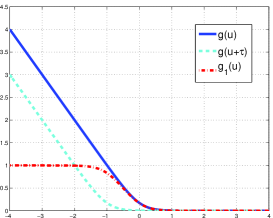
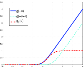
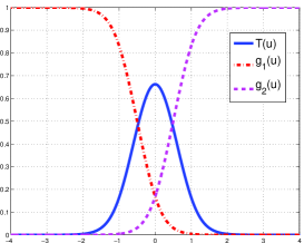
Figure 1: Example of a non-convex smooth transductive loss function $T(\cdot)$ obtained with $\tau=1$ as well as its components. (left) $g_{1}(u)$, (middle) $g_{2}(u)$, (right) DC decomposition of $T(u)$.

In this other experiment, we show an example of situation where one has to deal with a non-convex loss function as well as a non-convex regularizer, namely : sparse transductive logistic regression. The principle of transductive learning is to leverage unlabeled examples during the training step. This is usually done by using a loss function for unlabeled examples that enforces the decision function to lie in regions of low density. A way to achieve this is the use of a symmetric loss function which penalizes unlabeled examples lying in the margin of the classifier. It is well known that this approach, also known as low density separation, leads to non-convex data fitting term on the unlabeled examples [48]. For instance, Joachims [49] has considered a Symmetric Hinge loss for the unlabeled examples in their transductive implementation of SVM. Collobert et al. [38] extended this idea of symmetric Hinge loss into a symmetric ramp loss, which has a plateau on its top. In order to have a smooth transductive loss, Chapelle et al [48] used a symmetric sigmoid loss.

For our purpose the transductive loss function is required to be differentiable. Hence we propose the following symmetric differentiable loss that can be written as a difference of convex function

$$T(u)=1-g_{1}(u)-g_{2}(u)$$

where $g_{1}(u)=\frac{1}{\tau}(g(u)-g(u+\tau))$, $g_{2}(u)=g_{1}(-u)$ and $g(u)=\log(1+\exp(-u))$. Note that $g(u)$ is a convex function as depicted in Figure 1 and combinations of shifted and reversed versions of $g(u)$ lead to $g_{1}$ and $g_{2}$. $\tau$ is a parameter that modifies the smoothness of $T(\cdot)$. From the expression of $g_{1}$ and $g_{2}$, it is easy to retrieve the difference of convex functions form of $T(u)=T_{1}(u)-T_{2}(u)$ with $T_{1}(u)=1+\frac{1}{\tau}\left(g(u+\tau)+g(-u+\tau)\right)$ and $T_{2}(u)=\frac{1}{\tau}\left(g(u)+g(-u)\right)$. The transductive loss $T(\cdot)$ as well as $g_{1}$ and $g_{2}$ and their components are illustrated in Figure 1.

According to this definition of the transductive loss, for our experiments, we have used the following loss involving all training examples

$${{\color[rgb]{0,0,0}f(\mathbf{x})=}}\sum_{i=1}^{\ell}\log(1+\exp(-y_{i}\mathbf{a}_{i}^{\top}\mathbf{x}))+\gamma\sum_{j=1}^{\ell_{u}}T(\mathbf{b}_{j}^{\top}\mathbf{x})$$ (19)

$\{\mathbf{a}_{i},y_{i}\}$ being the labeled examples and $\{{\color[rgb]{0,0,0}\mathbf{b}}_{j}\}$ the unlabeled ones and $\gamma$ is an hyperparameter that balances the weight of both losses. As previously the capped-$\ell_{1}$ serves as a regularizer.

IV-B1 Toy dataset

In order to illustrate the benefit of our sparse transductive approach, we have considered the same toy dataset as in the previous subsection and the same experimental protocol. However, we have considered only $5$ relevant variables, sampled $100$ training examples and $5000$ testing examples. In addition, we have considered $10000$ unlabeled examples. The total number of variables is varying. We have compared the recognition performance of $3$ algorithms : the above-described capped-$\ell_{1}$ sparse logistic regression, the non-sparse transductive SVM (TSVM) of [48] and our sparse transductive logistic regression.

Evolution of the recognition rate of these algorithms with respects to the number of variables in the learning problem is depicted in Figure  2. Interestingly, when the number of variables is small enough, all algorithms perform equivalently. Then, as the number of (noisy) variables increases, the transductive SVM suffers a drop of performances. It seems more beneficial in this case to consider a model that is able to select relevant variables as our capped-$\ell_{1}$ sparse logistic regression still performs good. Best performances are obtained using our DC formulation introduced for solving the sparse transductive logistic regression problem which is able to remove noisy variables and take advantage of the unlabeled examples.

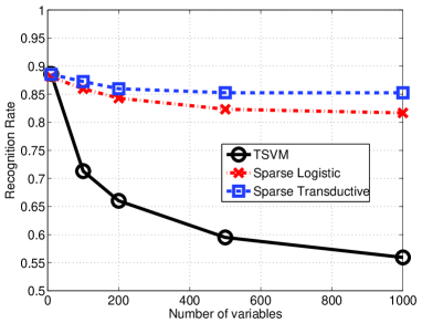
Figure 2: Recognition rate of different algorithms that are either sparse, transductive or both with respects to the number of variables in the problem, the number of relevant variables being $5$.

IV-B2 Benchmark datasets

We have also analyzed the benefit of using unlabeled examples in high-dimensional learning problems. For this experiment, all the hyperparameters of all models have been cross-validated. For instance, $\lambda$, $\theta$ (parameters of the capped $\ell_{1}$) and $\gamma$ have been respectively searched among the sets $\{0.2,2\}$, $\{0.2,2\}$ and $\{0.005,0.001,0.005,0.01\}$. averaged results over $10$ trials are reported in Table IV. Note that the results of the transductive SVM of [48] have not been reported because the provided code was not able to provide a solution in a reasonable amount of time. Results in Table IV show that being able to handle non-convex loss functions, related to the transductive loss and non-convex sparsity-inducing regularizers helps in achieving better performances in accuracy. Again, we can remark that the benefits of unlabeled examples are compelling especially when few labeled examples are in play. Differences in performances are indeed statistically significant for most datasets. In order to further evaluate the accuracy of the proposed method in very high-dimensional setting, we have run the comparison on the URL dataset. This dataset involves about $3.10^{6}$ features and we have learned a decision function using only $1000$ training examples and $40000$ unlabelled examples. Although difference in performances is not significant, leveraging on unsupervised examples helps in improving accuracy. Note that for this problem, the average running times of our DC-based sparse logistic regression and the DC-based sparse transductive regression are respectively about $500$ and $700$ seconds. This shows that the proposed approach allows to handle large-scale and very high-dimensional learning problems.

Table IV: Comparing the recognition rate of a sparse logistic regression and a sparse transductive logistic regression both with capped-$\ell_{1}$ regularizer. $\ell$ and $\ell_{u}$ respectively denotes the number of labeled and unlabeled examples.

			Class. Rate (%)
dataset	$d$	$\ell$	$\ell_{u}$	Sparse Log	Sparse Transd.
la2	31472	61	2398	67.65$\pm$2.6	70.23$\pm$3.1
sports	14870	85	6778	81.26$\pm$5.0	88.15$\pm$4.4
classic	41681	70	5604	72.74$\pm$4.3	86.97$\pm$2.2
ohscal	11465	55	8873	70.35$\pm$2.4	73.39$\pm$3.6
real-sim	20958	723	57124	88.81$\pm$0.3	88.91$\pm$1.4
url	3.23$\times 10^{6}$	1000	40000	86.64$\pm$5.8	87.39$\pm$6.0

V Conclusions

This paper introduced a general proximal Newton algorithm that optimizes the composite sum of functions. A specificity of the approach is its ability to deal with the non-convexity of both terms while one of these terms is in addition allowed to be non-differentiable. While most of the works in the machine learning and optimization communities have been addressing these non-differentiability and non-convexity issues separately, there exists a number of learning problems such as sparse transductive learning that require efficient optimization scheme on non-convex and non-differentiable functions. Our algorithm is based on two steps: the first one looks for a search direction through a proximal Newton step while the second one performs a line search on that direction. We also provide in this work the proof that the iterates generated by this algorithm behaves correctly in the sense that limit points of the sequences are stationary points. Numerical experiments show that the second order information used in our algorithm through the matrix $\mathbf{H}_{k}$ allow faster convergence than proximal gradient based descent approaches for non-convex regularizers. One of the strength of our framework is its ability to handle non-convexity on both the smooth loss function and the regularizer. We have illustrated this ability by learning a sparse transductive logistic regression model.

For the sake of reproducible research, the code source of the numerical simulation will be freely available on the authors website.

VI Appendix

VI-A Details on the proximal expression of $\Delta\mathbf{x}_{k}$

We provide in this paragraph the steps for obtaining Equation (7) from Equation (6).

Remind that for a lower semi-continuous convex function $h_{1}$, the proximal operator is defined as [15]

$$\mathbf{y}^{\star}={\textbf{prox}}_{h_{1}}^{\mathbf{H}}(\mathbf{x})=\arg\min_{\mathbf{y}}\frac{1}{2}\|\mathbf{y}-\mathbf{x}\|_{\mathbf{H}}^{2}+h_{1}(\mathbf{y})$$

$\mathbf{y}^{\star}$ can be characterized by the optimality condition of the optimization problem which is

$$-\mathbf{H}(\mathbf{y}^{\star}-\mathbf{x})\in\partial h_{1}(\mathbf{y}^{\star})$$

The search direction is provided by Equation (6) which we remind is

$$\operatorname*{arg\,min}_{\Delta\mathbf{x}}\frac{1}{2}\Delta\mathbf{x}^{\top}\mathbf{H}_{k}\Delta\mathbf{x}+h_{1}(\mathbf{x}_{k}+\Delta\mathbf{x})+{\mathbf{v}_{k}}^{\top}\Delta\mathbf{x}$$

By posing $\mathbf{z}=\mathbf{x}_{k}+\Delta\mathbf{x}$, we can equivalently look at a shifted version of this problem:

$$\mathbf{z}_{k}=\operatorname*{arg\,min}_{\mathbf{z}}\frac{1}{2}(\mathbf{z}-\mathbf{x}_{k})^{\top}\mathbf{H}_{k}(\mathbf{z}-\mathbf{x}_{k})+h_{1}(\mathbf{z})+\mathbf{v}_{k}^{\top}(\mathbf{z}-\mathbf{x}_{k})$$

Optimality condition of this problem is

$$-\mathbf{H}_{k}(\mathbf{z}_{k}-(\mathbf{x}_{k}-\mathbf{H}_{k}^{-1}\mathbf{v}_{k}))\in\partial h_{1}(\mathbf{z}_{k})$$

Hence, according to the optimality condition of the proximal operator, we have

$$\mathbf{z}_{k}={\textbf{prox}}_{h_{1}}^{\mathbf{H}}(\mathbf{x}_{k}-\mathbf{H}_{k}^{-1}\mathbf{v}_{k})$$

and thus

$$\Delta\mathbf{x}_{k}={\textbf{prox}}_{h_{1}}^{\mathbf{H}}(\mathbf{x}_{k}-\mathbf{H}_{k}^{-1}\mathbf{v}_{k})-\mathbf{x}_{k}$$

which is Equation (7).

VI-B Lemma 3 and proof

Lemma 3 : For $\mathbf{x}$ in the domain of $f$ and assuming that $\mathbf{H}_{k}\succeq m\mathbf{I}$ with $m>0$ and $\nabla f_{1}$ is Lipschitz with constant $L$ then the sufficient condition in Equation (17) holds for all $t_{k}$ so that

$$t_{k}\leq\min\left(1,2m\frac{1-\alpha}{L}\right)$$

Proof : Recall that $\mathbf{x}_{+}:=\mathbf{x}_{k}+t_{k}\Delta\mathbf{x}_{k}$. By definition, we have

$$F(\mathbf{x}_{+})-F(\mathbf{x}) =f_{1}(\mathbf{x}_{+})-f_{1}(\mathbf{x})-f_{2}(\mathbf{x}_{+})+f_{2}(\mathbf{x})$$

$$+h_{1}(\mathbf{x}_{+})-h_{1}(\mathbf{x})-h_{2}(\mathbf{x}_{+})+h_{2}(\mathbf{x}).$$

Then by convexity of $f_{2}$, $h_{2}$ and $h_{1}$, we derive that (see equation (14))

$$F(\mathbf{x}_{+})-F(\mathbf{x}) \leq f_{1}(\mathbf{x}_{+})-f_{1}(\mathbf{x})+(1-t)h_{1}(\mathbf{x})$$

$$\;\;+th_{1}(\mathbf{x}+\Delta\mathbf{x})-(\mathbf{z}_{f_{2}}+\mathbf{z}_{h_{2}})^{\top}(t\Delta\mathbf{x})$$

$$-h_{1}(\mathbf{x})$$

According to a Taylor-Laplace formulation, we have :

$$f_{1}(\mathbf{x}_{+})-f_{1}(\mathbf{x})=\int_{0}^{1}\nabla f_{1}(\mathbf{x}+st\Delta\mathbf{x})^{\top}(t\Delta\mathbf{x})ds$$

thus, we can rewrite

$$F(\mathbf{x}_{+})-F(\mathbf{x}) \leq\int_{0}^{1}\nabla f_{1}(\mathbf{x}+st\Delta\mathbf{x})^{\top}(t\Delta\mathbf{x})ds{\color[rgb]{0,0,0}-}th_{1}(\mathbf{x})$$

$$\;\;+th_{1}(\mathbf{x}+\Delta\mathbf{x})-(\mathbf{z}_{f_{2}}+\mathbf{z}_{h_{2}})^{\top}(t\Delta\mathbf{x})$$

$$\leq\int_{0}^{1}\Big{(}\nabla f_{1}(\mathbf{x}+st\Delta\mathbf{x})-\nabla f_{1}(\mathbf{x})\Big{)}^{\top}(t\Delta\mathbf{x})ds$$

$$\;\;+th_{1}(\mathbf{x}+\Delta\mathbf{x})+\nabla f_{1}(\mathbf{x})^{\top}(t\Delta\mathbf{x})$$

$$-(\mathbf{z}_{f_{2}}+\mathbf{z}_{h_{2}})^{\top}(t\Delta\mathbf{x})-th_{1}(\mathbf{x})$$

$$\leq t\Big{(}\int_{0}^{1}\Big{(}\nabla f_{1}(\mathbf{x}+st\Delta\mathbf{x})-\nabla f_{1}(\mathbf{x})\Big{)}^{\top}(\Delta\mathbf{x})ds$$

$$\;\;+h_{1}(\mathbf{x}+\Delta\mathbf{x})+\nabla f_{1}(\mathbf{x})^{\top}(\Delta\mathbf{x})$$

$$-(\mathbf{z}_{f_{2}}+\mathbf{z}_{h_{2}})^{\top}(\Delta\mathbf{x})-h_{1}(\mathbf{x})\Big{)}$$

Then using Cauchy-Schwartz inequality and the fact that $f_{1}$ is gradient Lipschitz of constant $L$, we have :

$$F(\mathbf{x}_{+})-F(\mathbf{x}) \leq t\Big{(}\int_{0}^{1}stL\|\Delta\mathbf{x}\|_{2}^{2}ds$$

$$\;\;+h_{1}(\mathbf{x}+\Delta\mathbf{x})+\nabla f_{1}(\mathbf{x})^{\top}(\Delta\mathbf{x})$$

$$-(\mathbf{z}_{f_{2}}+\mathbf{z}_{h_{2}})^{\top}(\Delta\mathbf{x})-h_{1}(\mathbf{x})\Big{)}$$

$$\leq t\Big{(}\frac{tL}{2}\|\Delta\mathbf{x}\|_{2}^{2}$$

$$\;\;+h_{1}(\mathbf{x}+\Delta\mathbf{x})+\nabla f_{1}(\mathbf{x})^{\top}(\Delta\mathbf{x})-$$

$$(\mathbf{z}_{f_{2}}+\mathbf{z}_{h_{2}})^{\top}(\Delta\mathbf{x})-h_{1}(\mathbf{x})\Big{)}$$

$$\leq t\Big{(}\frac{tL}{2}\|\Delta\mathbf{x}\|_{2}^{2}$$

$$\;\;+h_{1}(\mathbf{x}+\Delta\mathbf{x})-h_{1}(\mathbf{x}){\color[rgb]{0,0,0}+\mathbf{v}_{k}^{\top}(\Delta\mathbf{x})}\Big{)}$$

$$\leq t\Big{(}\frac{tL}{2}\|\Delta\mathbf{x}\|_{2}^{2}+D\Big{)}$$

Now, if $t$ is so that

$$t\leq 2m\frac{1-\alpha}{L}$$

then

$$\frac{Lt}{2}\|\Delta\mathbf{x}\|_{2}^{2} \leq m(1-\alpha)\|\Delta\mathbf{x}\|_{2}^{2}$$

$$=(1-\alpha)\Delta\mathbf{x}^{\top}(m\mathbf{I})\Delta\mathbf{x}$$

$$\leq(1-\alpha)\Delta\mathbf{x}^{\top}\mathbf{H}\Delta\mathbf{x}$$

$$\leq-(1-\alpha)D$$

where the last inequality comes from the descent property. Now, we plug this inequality back and get

$$t\Big{(}\frac{tL}{2}\|\Delta\mathbf{x}\|_{2}^{2}+D\Big{)}\leq t\Big{(}-(1-\alpha)D+D\Big{)}=t\alpha D$$

which concludes the proof that for all

$$t\leq\min\Big{(}1,2m\frac{1-\alpha}{L}\Big{)}$$

we have

$$F(\mathbf{x}_{+})-F(\mathbf{x})\leq t\alpha D$$

VI-C Convergence property for $F$ satisfying the KL property

Proposition 1 provides the general convergence property of our algorithm that applies to a large class of functions. Stronger convergence property (for instance, the convergence of the sequence $\{\mathbf{x}_{k}\}$ to a stationary point of $F(\mathbf{x})$) can be attained by restricting the class of functions and by imposing further conditions on the algorithms and some of its parameters. For instance, by considering functions $F(\mathbf{x})$ that satisfy the so-called Kurdyka-Lojasiewiszc property, convergence of the sequence can therefore be established.

Proposition 2

Assume the following assumptions:

• hypotheses on $f$ and $h$ given in section II are satisfied

• $h$ is continuous and defined over $\mathbb{R}^{d}$

• $\mathbf{H}_{k}$ is so that $\mathbf{H}_{k}\succeq m\mathbf{I}$ for all $k$ and $m>0$.

• $F$ is coercive and it satisfies the Kurdyka-Lojasiewicz property,

• $h_{2}$ verifies the $L_{2}$-Lipschitz gradient property, and thus there exists constant $L_{h_{2}}$

  $$\|\mathbf{u}-\mathbf{v}\|_{2}\leq L_{h_{2}}\|\mathbf{x}-\mathbf{y}\|_{2}\quad\mathbf{u}\in\partial h_{2}(\mathbf{x})\text{ and }\mathbf{v}\in\partial h_{2}(\mathbf{y})$$

• at each iteration, $\mathbf{H}_{k}$ is so that the function $\tilde{f}_{1}(\mathbf{z},\mathbf{x}_{k})=f_{1}(\mathbf{x}_{k})+\nabla f_{1}(\mathbf{x}_{k})^{\top}(\mathbf{z}-\mathbf{x}_{k})+\frac{1}{2}\|\mathbf{z}-\mathbf{x}_{k}\|^{2}_{\mathbf{H}_{k}}$ is a majorant approximation of $f_{1}(\cdot)$ i.e

  $$f_{1}(\mathbf{z})\leq\tilde{f}_{1}(\mathbf{z},\mathbf{x}_{k})\quad\forall\mathbf{z}$$

• there exists an $\tilde{\alpha}\in(0,1]$ so that at each iteration the condition

  $$F(\mathbf{x}_{k+1})\leq(1-\tilde{\alpha})F(\mathbf{x}_{k})+\tilde{\alpha}F(\mathbf{z}_{k})$$

  holds. Here, $\mathbf{z}_{k}$ is equal to $\mathbf{x}_{k}+\Delta\mathbf{x}$ as defined in Appendix A.

Under the above assumptions, the sequence $\{\mathbf{x}_{k}\}$ generated by our algorithm (1), converge to a critical point of $F=f+h$.

Before stating the proof, let us note that these conditions are quite restrictive and thus it may limit the scope of the convergence property. For instance, the hypothesis on $h_{2}$ holds for the SCAD regularizer but does not hold for the capped-$\ell_{1}$ penalty. We thus leave for future works the development of an adaptation of this proximal Newton algorithm for which convergence of the sequence $\{\mathbf{x}_{k}\}$ holds for a larger class of regularizers and loss functions.

Proof: The proof of convergence of sequence $\{\mathbf{x}_{k}\}$ strongly relies on Theorem 4.1 in [40]. Basically, this theorem states that sequences $\{\mathbf{x}_{k}\}$ generated by an algorithm minimizing a function $F=f+h$ with $h$ being convex and $F$ satisfying Kurdyka-Lojasiewicz property converges to a stationary point of $F$ under the above assumptions. The main difference between our framework and the one in [40] is that we consider a non-convex function $h(\mathbf{x})$. Hence, for a sake of brevity, we have given in what follows only some parts of the proofs given in [40] that needed to be reformulated due to the non-convexity of $h(\mathbf{x})$.

i) sufficient decrease property. This property provides similar guarantee than Lemma 4.1 in [40]. This property easily derives from Equations (17) and (15). Combining these two equations tells us that

$$F(\mathbf{x}_{k+1})-F(\mathbf{x}_{k})\leq-\alpha t_{k}\Delta\mathbf{x}^{\top}\mathbf{H}\Delta\mathbf{x}$$

where by definition, we have $\mathbf{x}_{k+1}=\mathbf{x}_{k}+t_{k}\Delta\mathbf{x}$. Thus, we get

$$F(\mathbf{x}_{k+1})-F(\mathbf{x}_{k}) \leq-\frac{\alpha}{t_{k}}\|\mathbf{x}_{k+1}-\mathbf{x}_{k}\|_{\mathbf{H}_{k}}^{2}$$

$$\leq-\frac{\alpha m}{t_{k}}\|\mathbf{x}_{k+1}-\mathbf{x}_{k}\|^{2}_{2}$$

$$\leq-\alpha m\|\mathbf{x}_{k+1}-\mathbf{x}_{k}\|^{2}_{2}$$

which proves that a sufficient decrease occurs at each iteration of our algorithm. In addition, because $\mathbf{x}_{k+1}-\mathbf{x}_{k}=t_{k}\Delta{\color[rgb]{0,0,0}\mathbf{x}}=t_{k}(\mathbf{z}_{k}-\mathbf{x}_{k})$, we also have

$$F(\mathbf{x}_{k+1})\leq F(\mathbf{x}_{k})-\alpha m\underline{t}^{2}\|\mathbf{z}_{k+1}-\mathbf{x}_{k}\|^{2}_{2}$$ (20)

where $\underline{t}$ is the smallest $t_{k}$ we may encounter. According to Lemma 3, we know that $\underline{t}>0$.

ii) convergence of $F(\mathbf{z}_{k})$ remind that we have defined $\mathbf{z}_{k}$ as (see appendix A)

$$\mathbf{z}_{k}=\operatorname*{arg\,min}_{\mathbf{z}}\frac{1}{2}(\mathbf{z}-\mathbf{x}_{k})^{\top}\mathbf{H}_{k}(\mathbf{z}-\mathbf{x}_{k})+h_{1}(\mathbf{z})+\mathbf{v}_{k}^{\top}(\mathbf{z}-\mathbf{x}_{k})$$

which is equivalent, by expanding $\mathbf{v}_{k}$ and adding constant terms, to

$$\min_{\mathbf{z}} \frac{1}{2}(\mathbf{z}-\mathbf{x}_{k})^{\top}\mathbf{H}_{k}(\mathbf{z}-\mathbf{x}_{k})+f_{1}(\mathbf{x}_{k})+\nabla f_{1}(\mathbf{x}_{k})^{\top}(\mathbf{z}-\mathbf{x}_{k})$$

$$-f_{2}(\mathbf{x}_{k})-\nabla f_{2}(\mathbf{x}_{k})^{\top}(\mathbf{z}-\mathbf{x}_{k})$$

$$-h_{2}(\mathbf{x}_{k})-\partial h_{2}(\mathbf{x}_{k})^{\top}(\mathbf{z}-\mathbf{x}_{k})$$

$$+h_{1}(\mathbf{z})$$

Note that the terms in the first line of this minimization problem majorize $f_{1}$ by hypotheses and the terms in the second and third lines respectively majorizes $-f_{2}$ and $-h_{2}$ since they are concave function. When we denotes as $Q(\mathbf{z},\mathbf{x}_{k})$ the objective function of the above problem, we have

$$F(\mathbf{z}_{k})\leq Q(\mathbf{z}_{k},\mathbf{x}_{k})<Q(\mathbf{x}_{k},\mathbf{x}_{k})=F(\mathbf{x}_{k})$$ (21)

where the first inequality holds because $Q(\mathbf{z},\mathbf{x}_{k})$ majorizes $F(\mathbf{z})$, the second one holds owing to the minimization. Combining this last equation with the assumption on $F(\mathbf{x}_{k+1})$, we have

$$\tilde{\alpha}^{-1}\big{(}F(\mathbf{x}_{k+1})-(1-\tilde{\alpha})F(\mathbf{x}_{k})\big{)}\leq F(\mathbf{z}_{k})\leq F(\mathbf{x}_{k})$$

This last equation allows us to conclude that if $F(\mathbf{x}_{k})$ converges to a real $\xi$, then $F(\mathbf{z}_{k})$ converges to $\xi$.

iii) bounding subgradient at $F(\mathbf{z}_{k})$

A subgradient $\mathbf{z}_{F}$ of $F$ at a given $\mathbf{z}_{k}$ is by definition

$$\mathbf{z}_{F}=\nabla f_{1}(\mathbf{z}_{k})-\nabla f_{2}(\mathbf{z}_{k})+\mathbf{z}_{h_{1},z_{k}}-\mathbf{z}_{h_{2},z_{k}}$$

where $\mathbf{z}_{h_{1},z_{k}}\in\partial h_{1}(\mathbf{z}_{k})$ and $\mathbf{z}_{h_{2},z_{k}}\in\partial h_{2}(\mathbf{z}_{k})$. Hence, we have

$$\|\mathbf{z}_{F}\|\leq \|\nabla f_{1}(\mathbf{z}_{k})-\nabla f_{1}(\mathbf{x}_{k})\|+\|\nabla f_{2}(\mathbf{z}_{k})-\nabla f_{2}(\mathbf{x}_{k})\|$$

$$+\|\mathbf{z}_{h_{2},z_{k}}-\mathbf{z}_{h_{2}}\|$$

$$+\|\nabla f_{1}(\mathbf{x}_{k})-\nabla f_{2}(\mathbf{x}_{k})+\mathbf{z}_{h_{1},z_{k}}-\mathbf{z}_{h_{2}}\|$$

In addition, owing to the optimality condition of $\mathbf{z}_{k}$, the following hold

$$\mathbf{H}_{k}(\mathbf{z}_{k}-\mathbf{x}_{k})=\nabla f_{1}(\mathbf{x}_{k})-\nabla f_{2}(\mathbf{x}_{k})+\mathbf{z}_{h_{1},z_{k}}-\mathbf{z}_{h_{2}}$$

Hence, owing to the Lipschitz gradient hypothesis of $f_{1}$ and $f_{2}$ and the hypothesis on $h_{2}$, there exists a constant $\mu>0$ such that

$$\|\mathbf{z}_{F}\|\leq\mu\|\mathbf{z}_{k}-\mathbf{x}_{k}\|$$ (22)

References

- [1] R. Tibshirani, “Regression shrinkage and selection via the lasso,” Journal of the Royal Statistical Society, vol. 58, no. 1, pp. 267–288, 1996.
- [2] S. Chen, D. Donoho, and M. Saunders, “Atomic decomposition by basis pursuit,” SIAM Journal Scientific Comput., vol. 20, no. 1, pp. 33–61, 1999.
- [3] Y. Li and S.-I. Amari, “Two conditions for equivalence of 0-norm solution and 1-norm solution in sparse representation,” Neural Networks, IEEE Transactions on, vol. 21, no. 7, pp. 1189–1196, Jul. 2010.
- [4] D. Donoho, “For most large underdetermined systems of linear equations, the minimal solution is also the sparsest solution,” Communication in Pure and Applied Mathematics, vol. 59, no. 6, pp. 797–829, 2006.
- [5] S. Shevade and S. Keerthi, “A simple and efficient algorithm for gene selection using sparse logistic regression,” Bioinformatics, vol. 19, no. 17, pp. 2246–2253, 2003.
- [6] A. Beck and M. Teboulle, “A fast iterative shrinkage-thresholding algorithm for linear inverse problems,” SIAM Journal on Imaging Sciences, vol. 2, no. 1, pp. 183–202, 2009.
- [7] G.-X. Yuan, C.-H. Ho, and C.-J. Lin, “An improved glmnet for l1-regularized logistic regression,” The Journal of Machine Learning Research, vol. 13, pp. 1999–2030, Jun. 2013.
- [8] F. Bach, R. Jenatton, J. Mairal, and G. Obozinski, “Convex optimization with sparsity-inducing norms,” in Optimization for Machine Learning, S. Sra, S. Nowozin, and S. Wright, Eds. MIT Press, 2011.
- [9] H. Zou, “The adaptive lasso and its oracle properties,” Journal of the American Statistical Association, vol. 101, no. 476, pp. 1418–1429, 2006.
- [10] J. Fan and R. Li, “Variable selection via nonconcave penalized likelihood and its oracle properties,” Journal of the American Statistical Association, vol. 96, no. 456, pp. 1348–1360, 2001.
- [11] K. Knight and W. Fu, “Asymptotics for lasso-type estimators,” Annals of Statistics, vol. 28, no. 5, pp. 1356–1378, 2000.
- [12] E. Candès, M. Wakin, and S. Boyd, “Enhancing sparsity by reweighted minimization,” J. Fourier Analysis and Applications, vol. 14, no. 5-6, pp. 877–905, 2008.
- [13] L. Laporte, R. Flamary, S. Canu, S. Dejean, and J. Mothe, “Nonconvex regularizations for feature selection in ranking with sparse svm,” Neural Networks and Learning Systems, IEEE Transactions on, vol. 25, no. 6, pp. 1118–1130, 2014.
- [14] G. Gasso, A. Rakotomamonjy, and S. Canu, “Recovering sparse signals with a certain family of non-convex penalties and dc programming,” IEEE Trans. Signal Processing, vol. 57, no. 12, pp. 4686–4698, 2009.
- [15] P. L. Combettes and J.-C. Pesquet, “Proximal splitting methods in signal processing,” in Fixed-Point Algorithms for Inverse Problems in Science and Engineering, H. H. Bauschke, R. Burachik, P. L. Combettes, V. Elser, D. R. Luke, and H. Wolkowicz, Eds. Springer-Verlag, 2011, pp. 185–212.
- [16] J. Lee, Y. Sun, and M. Saunders, “Proximal newton-type methods for convex optimization,” in Advances in Neural Information Processing Systems, Lake Tahoe, NV, Dec. 2012, pp. 836–844.
- [17] S. Becker and J. Fadili, “A quasi-newton proximal splitting method,” in Advances in Neural Information Processing Systems, Lake Tahoe, NV, Dec. 2012, pp. 2618–2626.
- [18] H. A. Le Thi and T. Pham Dinh, “The dc (difference of convex functions) programming and dca revisited with dc models of real world nonconvex optimization problems,” Annals of Operations Research, vol. 133, no. 1-4, pp. 23–46, 2005.
- [19] T. Pham Dinh and H. A. Le Thi, “Convex analysis approach to dc programming: Theory, algorithms and applications,” Acta Mathematica Vietnamica, vol. 22, no. 1, pp. 287–355, 1997.
- [20] F. Akoa, “Combining dc algorithms (dcas) and decomposition techniques for the training of nonpositive semidefinite kernels,” Neural Networks, IEEE Transactions on, vol. 19, no. 11, pp. 1854–1872, Nov 2008.
- [21] R. Jenatton, J. Mairal, G. Obozinski, and F. Bach, “Proximal methods for sparse hierarchical dictionary learning,” in Proceedings of International Conference on Machine Learning, Tel Aviv, Israel, Jun. 2010, pp. 487–494.
- [22] A. Rakotomamonjy, “Direct optimization of the dictionary learning problem,” IEEE Trans. on Signal Processing, vol. 61, no. 12, pp. 5495–5506, 2013.
- [23] N. Srebro, J. Rennie, and T. S. Jaakkola, “Maximum-margin matrix factorization,” in Advances in neural information processing systems, no. Vancouver, BC, Dec., 2004, pp. 1329–1336.
- [24] S. Ertekin, L. Bottou, and C. Giles, “Nonconvex online support vector machines,” IEEE Trans. on Pattern Analysis and Machine Intelligence, vol. 33, no. 2, pp. 368–381, 2011.
- [25] R. Collobert, F. Sinz, J. Weston, and L. Bottou, “Trading convexity for scalability,” in Proceedings of the Twenty-third International Conference on Machine Learning (ICML 2006). ACM Press, 2006, pp. 201–208.
- [26] A. L. Yuille, A. Rangarajan, and A. Yuille, “The concave-convex procedure (cccp),” Advances in neural information processing systems, vol. 2, pp. 1033–1040, Vancouver, BC, Dec. 2002.
- [27] N. Courty, R. Flamary, and D. Tuia, “Domain adaptation with regularized optimal transport,” in Machine Learning and Knowledge Discovery in Databases. Springer, Nancy, France, Sep. 2014, pp. 274–289.
- [28] R. Jenatton, G. Obozinski, and F. Bach, “Structured sparse principal component analysis.” in Proceedings of the International Conference on Artificial Intelligence and Statistics, Y. W. Teh and D. M. Titterington, Eds., vol. 9, Chia, Italy, May 2010, pp. 366–373.
- [29] E. Richard, P.-A. Savalle, and N. Vayatis, “Estimation of simultaneously sparse and low rank matrices.” in Proceedings of the International Conference in Machine Learning. Omnipress, Edinburgh, Scotland, Jun. 2012.
- [30] Y. Deng, Q. Dai, R. Liu, Z. Zhang, and S. Hu, “Low-rank structure learning via nonconvex heuristic recovery,” Neural Networks and Learning Systems, IEEE Transactions on, vol. 24, no. 3, pp. 383–396, 2013.
- [31] K. Zhong, E.-H. Yen, I. S. Dhillon, and P. K. Ravikumar, “Proximal quasi-newton for computationally intensive l1-regularized m-estimators,” in Advances in Neural Information Processing Systems 27, Z. Ghahramani, M. Welling, C. Cortes, N. Lawrence, and K. Weinberger, Eds. Curran Associates, Inc., Montreal, Canada, Dec. 2014, pp. 2375–2383.
- [32] M. Figueiredo, R. Nowak, and S. Wright, “Gradient projection for sparse reconstruction: application to compressed sensing and other inverse problems,” IEEE Journal of Selected Topics in Signal Processing: Special Issue on Convex Optimization Methods for Signal Processing, vol. 1, no. 4, pp. 586–598, 2007.
- [33] G. Golub and C. Van Loan, Matrix computations. Johns Hopkins University Press, 1996, vol. 3.
- [34] P. Gong, C. Zhang, Z. Lu, J. Huang, and Y. Jieping, “A general iterative shrinkage and thresholding algorithm for non-convex regularized optimization problems,” in Proceedings of the 30th International Conference on Machine Learning, Atlanta, Georgia, Jun. 2013, pp. 37–45.
- [35] Z. Lu, “Sequential convex programming methods for a class of structured nonlinear programming,” ArXiv:1210.3039, Tech. Rep., 2012.
- [36] P.-L. Loh and M. J. Wainwright, “Regularized m-estimators with nonconvexity: Statistical and algorithmic theory for local optima,” in Advances in Neural Information Processing Systems 26, C. Burges, L. Bottou, M. Welling, Z. Ghahramani, and K. Weinberger, Eds., Lake Tahoe, NV, Dec 2013, pp. 476–484.
- [37] T. Pham Dinh and H. A. Le Thi, “Dc optimization algorithms for solving the trust region subproblem,” SIAM Journal of Optimization, vol. 8, pp. 476–505, 1998.
- [38] R. Collobert, F. Sinz, J. Weston, and L. Bottou, “Large scale transductive svms,” Journal of Machine Learning Research, vol. 7, pp. 1687–1712, 2006.
- [39] H. Mine and M. Fukushima, “A minimization method for the sum of a convex function and a continuously differentiable function,” Journal of Optimization Theory and Applications, vol. 33, no. 1, pp. 9–23, 1981.
- [40] E. Chouzenoux, J.-C. Pesquet, and A. Repetti, “Variable metric forward–backward algorithm for minimizing the sum of a differentiable function and a convex function,” Journal of Optimization Theory and Applications, vol. 162, no. 1, pp. 107–132, 2014.
- [41] S. Sra, “Scalable nonconvex inexact proximal splitting,” in Advances in Neural Information Processing Systems, Lake Tahoe, NV, Dec. 2012, pp. 530–538.
- [42] H. Attouch, J. Bolte, P. Redont, and A. Soubeyran, “Proximal alternating minimization and projection methods for nonconvex problems: an approach based on the Kurdyka-Lojasiewicz inequality,” Mathematics of Operations Research, vol. 35, no. 2, pp. 438–457, 2010.
- [43] H. Attouch, J. Bolte, and B. F. Svaiter, “Convergence of descent methods for semi-algebraic and tame problems: proximal algorithms, forward–backward splitting, and regularized gauss–seidel methods,” Mathematical Programming, vol. 137, no. 1-2, pp. 91–129, 2013.
- [44] J. Bolte, S. Sabach, and M. Teboulle, “Proximal alternating linearized minimization for nonconvex and nonsmooth problems,” Mathematical Programming, vol. 146, no. 1-2, pp. 459–494, 2014.
- [45] T. Zhang, “Analysis of multi-stage convex relaxation for sparse regularization,” Journal of Machine Learning Researc, vol. 11, pp. 1081–1107, 2010.
- [46] A. Boisbunon, R. Flamary, and A. Rakotomamonjy, “Active set strategy for high-dimensional non-convex sparse optimization problems,” in Acoustics, Speech and Signal Processing (ICASSP), IEEE International Conference on. IEEE, Firenze, Italy, May 2014, pp. 1517–1521.
- [47] A. Rakotomamonjy, R. Flamary, G. Gasso, and S. Canu, “ penalty for sparse linear and sparse multiple kernel multi-task learning,,” IEEE Trans. on Neural Networks, vol. 22, no. 8, pp. 1307–1320, 2011.
- [48] O. Chapelle and A. Zien, “Semi-supervised classification by low density separation,” in Proceedings of the Tenth International Workshop on Artificial Intelligence and Statistic, Barbados, Jan. 2005, pp. 57–64.
- [49] T. Joachims, “Transductive inference for text classification using svms,” in Proceedings of The 16th International Conference on Machine Learning, vol. 99, Bled, Slovenia, Jun. 1999, pp. 200–209.