Resurgence in sine-Gordon quantum mechanics:
Exact agreement between multi-instantons and uniform WKB

Abstract

We compute multi-instanton amplitudes in the sine-Gordon quantum mechanics (periodic cosine potential) by integrating out quasi-moduli parameters corresponding to separations of instantons and anti-instantons. We propose an extension of Bogomolnyi–Zinn-Justin prescription for multi-instanton configurations and an appropriate subtraction scheme. We obtain the multi-instanton contributions to the energy eigenvalue of the lowest band at the zeroth order of the coupling constant. For the configurations with only instantons (anti-instantons), we obtain unambiguous results. For those with both instantons and anti-instantons, we obtain results with imaginary parts, which depend on the path of analytic continuation. We show that the imaginary parts of the multi-instanton amplitudes precisely cancel the imaginary parts of the Borel resummation of the perturbation series, and verify that our results completely agree with those based on the uniform-WKB calculations, thus confirming the resurgence : divergent perturbation series combined with the nonperturbative multi-instanton contributions conspire to give unambiguous results. We also study the neutral bion contributions in the ${\mathbb{C}}P^{N-1}$ model on ${\mathbb{R}}^{1}\times S^{1}$ with a small circumference, taking account of the relative phase moduli between the fractional instanton and anti-instanton. We find that the sign of the interaction potential depends on the relative phase moduli, and that both the real and imaginary parts resulting from quasi-moduli integral of the neutral bion get quantitative corrections compared to the sine-Gordon quantum mechanics.

I Introduction

In the recent study on quantum field theories and quantum mechanics, topologically neutral soliton molecules, which are locally composed of (fractional) instantons and anti-instantons, have been attracting a great deal of attention in relation to the IR-renormalonUnsal:2007vu ; Unsal:2007jx ; Shifman:2008ja ; Poppitz:2009uq ; Anber:2011de ; Poppitz:2012sw ; Argyres:2012vv ; Argyres:2012ka ; Dunne:2012ae ; Dunne:2012zk ; Dabrowski:2013kba ; Dunne:2013ada ; Cherman:2013yfa ; Basar:2013eka ; Dunne:2014bca ; Cherman:2014ofa ; Behtash:2015kna ; Bolognesi:2013tya ; Misumi:2014jua ; Misumi:2014raa ; Misumi:2014bsa ; Nitta:2015tua ; Nitta:2014vpa ; Shermer:2014wxa ; Dunne:2015ywa . Imaginary ambiguities arising in amplitudes of such topologically neutral configurations can cancel out those arising in non-Borel-summable perturbative series (IR-renormalon) in quantum theories under certain conditions on the spacetime manifold Argyres:2012vv ; Argyres:2012ka ; Dunne:2012ae ; Dunne:2012zk ; Dabrowski:2013kba ; Dunne:2013ada ; Cherman:2013yfa ; Basar:2013eka ; Dunne:2014bca ; Cherman:2014ofa ; Bolognesi:2013tya ; Misumi:2014jua ; Misumi:2014raa ; Misumi:2014bsa ; 'tHooft:1977am ; Fateev:1994ai ; Fateev:1994dp . In field theories on compactified spacetime with a small compact dimension, these objects are termed as “bions” Argyres:2012vv ; Argyres:2012ka ; Dunne:2012ae ; Dunne:2012zk . It is expected that full semi-classical expansion including perturbative and non-perturbative sectors as bions, which is called “resurgent” expansion Ec1 ; Marino:2007te ; Marino:2008ya ; Marino:2008vx ; Pasquetti:2009jg ; Drukker:2010nc ; Aniceto:2011nu ; Marino:2012zq ; Hatsuda:2013gj ; Schiappa:2013opa ; Hatsuda:2013oxa ; Aniceto:2013fka ; Santamaria:2013rua ; Kallen:2013qla ; Honda:2014ica ; Grassi:2014cla ; Sauzin ; Kallen:2014lsa ; Couso-Santamaria:2014iia ; Honda:2014bza ; Aniceto:2014hoa ; Couso-Santamaria:2015wga ; Honda:2015ewa ; Hatsuda:2015owa ; Aniceto:2015rua ; Dorigoni:2015dha , leads to unambiguous and self-consistent definition of field theories in the same manner as the conjecture in quantum mechanics Bogomolny:1980ur ; ZinnJustin:1981dx ; ZinnJustin:1982td ; ZinnJustin:1983nr ; ZinnJustin:2004ib ; ZinnJustin:2004cg ; Jentschura:2010zza .

The resurgence in theoretical physics was at first investigated in the matrix model and topological string theory Marino:2007te ; Marino:2008ya ; Marino:2008vx ; Pasquetti:2009jg ; Marino:2012zq ; Hatsuda:2013oxa . Then, the study on the topic has been extended to ABJM theory Drukker:2010nc ; Hatsuda:2013gj ; Honda:2014ica ; Kallen:2014lsa , string and supersymmetric gauge theories Aniceto:2011nu ; Grassi:2014cla ; Couso-Santamaria:2014iia ; Aniceto:2014hoa , and general quantum systems Schiappa:2013opa ; Aniceto:2013fka ; Santamaria:2013rua ; Kallen:2013qla ; Sauzin ; Honda:2014bza ; Couso-Santamaria:2015wga ; Honda:2015ewa ; Hatsuda:2015owa ; Aniceto:2015rua ; Dorigoni:2015dha . Bions and resurgence in non-SUSY field theories, especially in the low-dimensional models, have been extensively investigated for the ${\mathbb{C}}P^{N-1}$ model Dunne:2012ae ; Dunne:2012zk ; Dabrowski:2013kba ; Bolognesi:2013tya ; Misumi:2014jua ; Shermer:2014wxa , the Grassmann sigma model Misumi:2014bsa ; Dunne:2015ywa , the principal chiral model Cherman:2013yfa ; Cherman:2014ofa ; Nitta:2015tua , and the $O(N)$ model Nitta:2014vpa ; Dunne:2015ywa . According to these studies, the leading-order renormalon ambiguity $\mp i\pi e^{-2S_{I}/N}$ arising in non-Borel-summable perturbative series, which corresponds to the singularity closest to the origin on the Borel plane, is compensated by the amplitude of neutral bions. On the other hand, it is expected but not verified that the ambiguities corresponding to singularities further from the origin ($\mp i\pi e^{-4S_{I}/N}$, $\mp i\pi e^{-6S_{I}/N}$,…) are cancelled by amplitudes of bion molecules with more than four instanton constituents.

In the case of quantum mechanics, not only the sector of zero instanton charge but also those of nonzero instanton charge contribute to physical observables such as the energy levels. The authors in Refs. ZinnJustin:1981dx ; ZinnJustin:1982td ; ZinnJustin:1983nr ; ZinnJustin:2004ib ; ZinnJustin:2004cg ; Jentschura:2010zza investigated quantum mechanics with several types of potential including the sine-Gordon type. They showed that the leading instanton contributions are consistent with the perturbative calculation, and conjectured the explicit equation connecting perturbative and instanton contributions, which they call the generalized quantization condition. Recently the authors in Refs. Dunne:2013ada ; Dunne:2014bca adopted the uniform-WKB method based on the boundary condition, which is equivalent to the quantization condition in Refs. ZinnJustin:1981dx ; ZinnJustin:1982td ; ZinnJustin:1983nr ; ZinnJustin:2004ib ; ZinnJustin:2004cg ; Jentschura:2010zza , and pointed out the general relation between perturbative and non-perturbative contributions. Explicit calculations of multi-instanton amplitudes at each configuration level are expected to clarify the structure of resurgence and to verify the conjectured relation between perturbative and non-perturbative contributions ZinnJustin:1981dx ; ZinnJustin:1982td ; ZinnJustin:1983nr ; ZinnJustin:2004ib ; ZinnJustin:2004cg ; Jentschura:2010zza ; Escobar-Ruiz:2015nsa ; Dunne:2013ada ; Dunne:2014bca .

In this paper, we focus on a quantum mechanical system with the sine-Gordon potential, and we calculate the multi-instanton amplitude by explicitly integrating quasi moduli parameters corresponding to separations of instanton-constituents in a semi-classical limit, in comparison with the uniform WKB calculations Dunne:2013ada ; Dunne:2014bca ; ZinnJustin:2004ib ; ZinnJustin:2004cg . We adopt an extension of Bogomolnyi–Zinn-Justin prescription Bogomolny:1980ur ; ZinnJustin:1981dx for multi-instanton configurations with an appropriate subtraction scheme for divergent parts. We calculate contributions to the energy eigenvalue of the lowest band from each multi-instanton configuration in a semi-classical limit ($|g^{2}|\ll 1$). For the configurations with only instantons (anti-instantons) such as $[\mathcal{I}\mathcal{I}]$, $[\mathcal{I}\mathcal{I}\mathcal{I}]$ and $[\mathcal{I}\mathcal{I}\mathcal{I}\mathcal{I}]$, we have unambiguous results without imaginary parts. Here, we have denoted an instanton (anti-instanton) as $\mathcal{I}$ ($\bar{\mathcal{I}}$). For configurations containing both instantons and anti-instantons such as $[\mathcal{I}\bar{\mathcal{I}}]$, $[\mathcal{I}\mathcal{I}\bar{\mathcal{I}}]$ and $[\mathcal{I}\mathcal{I}\bar{\mathcal{I}}\bar{\mathcal{I}}]$, the results contain ambiguous imaginary parts, which depend on the path of analytic continuation. These imaginary parts correspond to the large-order behavior of perturbation series around the saddle point without the $[\mathcal{I}\bar{\mathcal{I}}]$ pair. For instance, we show explicitly that the imaginary part of the multi-instanton amplitude $[\mathcal{I}\mathcal{I}\bar{\mathcal{I}}]$ cancels the imaginary part of the Borel resummation of the large-order perturbation series around the nontrivial background with a single instanton $[\mathcal{I}]$. By investigating the uniform-WKB calculations in detail, we verify that all of our results agree completely with those based on the uniform-WKB calculations up to a four-instanton order.

While the sine-Gordon quantum mechanics is worth to study on its own, another strong motivation lies in its close relationship to small circumference limit of the two-dimensional ${\mathbb{C}}P^{N-1}$ model on ${\mathbb{R}}^{1}\times S^{1}$ (circumference $L$) with the ${\mathbb{Z}}_{N}$-symmetric twisted boundary condition Dunne:2012ae ; Dunne:2012zk . However, we observe that some of the field configurations of the ${\mathbb{C}}P^{N-1}$ model are not faithfully represented by means of the sine-Gordon quantum mechanics. One can derive the sine-Gordon quantum mechanics from the two-dimensional ${\mathbb{C}}P^{N-1}$ model by applying the Scherk-Schwarz dimensional reduction, which requires a particular dependence of the phases of fields on the coordinate $x_{2}$ of compactified dimension ($0\leq x_{2}<L$). It is important to realize that only parts of field configuration of ${\mathbb{C}}P^{N-1}$ model can be consistent with this $x_{2}$ dependence. For instance, the BPS solution of two fractional instantons is not consistent with the Scherk-Schwarz reduction, and hence its small circumference limit cannot be described by the sine-Gordon quantum mechanics. On the other hand, two adjacent instantons in the sine-Gordon quantum mechanics are mutually non-BPS, although each individual instanton may be understood as a limit of BPS fractional instanton (with a different $x_{2}$ dependence). Even in the instanton and anti-instanton configurations, ${\mathbb{C}}P^{N-1}$ model has a significant difference compared to the sine-Gordon quantum mechanics: The phase moduli of the fractional instantons in the ${\mathbb{C}}P^{N-1}$ model are neglected in the sine-Gordon quantum mechanics. For the configuration of a neutral bion composed of a fractional instanton and an anti-fractional instanton, we find that the interaction between them strongly depends on the relative phase of constituents. We calculate the neutral bion contribution in the ${\mathbb{C}}P^{N-1}$ model, based on the interaction potential with the quasi moduli parameter corresponding to the relative phase between the fractional instanton and anti-instanton. We find that this calculation gives a correction factor compared to the neutral bion amplitude obtained in the sine-Gordon quantum mechanics Dunne:2012ae ; Dunne:2012zk .

This paper is organized as follows. In Sec. II, we review instantons and their interactions in the quantum mechanics with sine-Gordon potential and the Borel summation. In Sec. III we calculate amplitudes of multi-instanton configurations in sine-Gordon quantum mechanics by integrating out the moduli parameters. In Sec. IV we discuss the results from the uniform WKB calculations, and show that they completely agree with the instanton moduli calculations. In Sec. V we discuss the neutral bion contributions in the compactified ${\mathbb{C}}P^{N-1}$ model based on the interaction potential including the relative phase parameter. Section VI is devoted to a summary and discussion. In Appendix A we give some details of four-instanton calculations.

II Quantum mechanics with the sine-Gordon potential

In this article, we focus on the sine-Gordon quantum mechanics described by the Schrödinger equation

$$H\psi(x)=-{1\over{2}}{d^{2}\over{dx^{2}}}\psi(x)\,+\,{1\over{8g^{2}}}\sin^{2}(2gx)\,\psi(x)\,=\,E\,\psi(x)\,,$$ (1)

where we follow the notation in Refs. ZinnJustin:2004ib ; Dunne:2013ada except $g$ is replaced by $g^{2}$ here . The Euclidian Lagrangian for the sine-Gordon quantum mechanics is given by

$$L\,=\,{1\over{2}}\left({dx\over{dt}}\right)^{2}\,+\,V(x),\qquad V(x)={1\over{8g^{2}}}\sin^{2}(2gx)\,.$$ (2)

In the $g^{2}\to 0$ limit, it reduces to the Schrödinger equation of the harmonic oscillator.

The energy eigenvalues of periodic potentials split into bands of states. Within each band, they are labeled by the Bloch angle $\theta\in[0,\pi]$ defined by

$$\psi\left(x+\frac{\pi}{2g}\right)\,=\,e^{i\theta}\psi(x)\,.$$ (3)

In this article, we are interested in the lowest band, although excited bands can be treated similarly. The energy eigenvalue $E$ of the lowest band can be expressed in terms of the path-integral

$$E=\lim_{\beta\to\infty}\frac{-1}{\beta}{\rm Tr}e^{-\beta H}=\lim_{\beta\to\infty}\frac{-1}{\beta}\int_{x(t=-\beta/2)=x(t=\beta/2)}Dx(t)\,e^{-S+iQ\theta}.$$ (4)

For weak coupling, the path-integral has contributions $E_{\rm pert}(g^{2})$ around the perturbative vacuum, as well as contributions $\triangle E$ from nonperturbative saddle points

$$E=E_{\rm pert}(g^{2})+\triangle E.$$ (5)

Perturbation series in powers of coupling constant $g^{2}$ in quantum field theories or in quantum mechanics are extremely useful, but are usually factorially divergent

$$E_{\rm pert}(g^{2})=\sum_{K=0}^{\infty}a_{K}(g^{2})^{K},\qquad a_{K}\sim K!\;.$$ (6)

It is useful to define the Borel transform $B_{\rm pert}(t)$

$$B_{\rm pert}(t)=\sum_{K=0}^{\infty}\frac{a_{K}}{K!}t^{K}.$$ (7)

The Borel resummation ${\mathbb{E}}_{\rm pert}(g^{2})$ of the divergent series $E_{\rm pert}(g^{2})$ is defined as an integral of the Borel transform along the positive real axis in the complex Borel plane $t$

$${\mathbb{E}}_{\rm pert}(g^{2})=\int_{0}^{\infty}{dt}e^{-t}B_{\rm pert}(g^{2}t).$$ (8)

If the factorially divergent series is alternating, the Borel transform has no singularities along the positive real $t$ axis, and the Borel resummation becomes well-defined (Borel-summable). For the potential with degenerate minima such as the sine-Gordon quantum mechanics, however, the perturbation series is non-alternating factorially divergent. In that case, the Borel transform is convergent with the finite radius of convergence, but the Borel resummation is ill-defined because of singularities in the complex Borel plane. Since the series become alternating and the Borel resummation ${\mathbb{E}}_{\rm pert}(g^{2})$ is unambiguous for $-g^{2}>0$, we can analytically continue it from $-g^{2}>0$ to the physical region $g^{2}>0$ to obtain a real analytic function ${\mathbb{E}}_{\rm pert}(g^{2})$. If there is no complex singularities, we obtain a branch cut along the positive real axis of complex $g^{2}$ plane. The imaginary part ${\rm Im}{\mathbb{E}}_{\rm pert}(g^{2})$ at $g^{2}>0$ is related to the large-order behavior ($K\gg 1$) of perturbation series $E_{\rm pert}(g^{2})$ in Eq.(6) through the dispersion relation ZinnJustin:1989mi

$$a_{K}\,\approx\,{-1\over{\pi}}\int_{0}^{\infty}\,dg^{2}\,\frac{[{\rm Im}{\mathbb{E}}_{\rm pert}(g^{2})]}{(g^{2})^{K+1}}.$$ (9)

This large-order behavior corresponds to the singularities of the Borel transform $B_{\rm pert}(g^{2}t)$ in the complex Borel plane $t$. Of course this ambiguous (path-dependent) imaginary part is unacceptable, and should disappear, since the energy eigenvalue $E$ should be real, and ambiguity due to the choice of path is unphysical. In fact, it has been found that the leading term of the imaginary ambiguities is cancelled by the contributions from non-perturbative saddle points associated with neutral objects composed of instantons Dunne:2013ada ; Dunne:2014bca . This phenomenon is called the resurgence of the perturbation series.

Let us now consider non-perturbative saddle points. By rescaling the variable

$$2gx=y,$$ (10)

the Euclidean Lagrangian in Eq.(2) can be rewritten as

$$L\,=\,{1\over{8g^{2}}}\left({dy\over{dt}}\right)^{2}\,+\,V,\qquad V={1\over{8g^{2}}}\sin^{2}(y)\,.$$ (11)

and the instanton number as a topological charge may be defined by

$$Q=\frac{1}{\pi}\int_{-\infty}^{\infty}dt\,\frac{dy}{dt}\,.$$ (12)

Single instanton solution ($Q=1$) is given by

$$y_{\mathcal{I}}(t)=2\arctan e^{t-t_{0}}+n\pi,\quad n\in{\mathbb{Z}},$$ (13)

whereas single anti-instanton solution ($Q=-1$) is given by

$$y_{\bar{\mathcal{I}}}(t)=2\arctan e^{-(t-t_{0})}+(n-1)\pi,\quad n\in{\mathbb{Z}},$$ (14)

with the Euclidean action

$$S_{\mathcal{I}}\,=\,{1\over{2g^{2}}}\,.$$ (15)

The moduli parameter $t_{0}$ is a zero mode (moduli) associated to the breakdown of translation, representing the location of the (anti-)instanton. For even $n$, the solutions (13) and (14) satisfy the following BPS equation saturating the BPS bound for $S$

$$\frac{dy}{dt}=\sin y,\quad S=\int_{-\infty}^{\infty}dt\frac{dy}{dt}\sin y.$$ (16)

For odd $n$, they satisfy the anti-BPS equation saturating the anti-BPS bound for $S$

$$\frac{dy}{dt}=-\sin y,\quad S=-\int_{-\infty}^{\infty}dt\frac{dy}{dt}\sin y.$$ (17)

By integrating over the translational zero mode $t_{0}$, one finds the contribution $\triangle E^{(1,0)}$ of single instanton $[\mathcal{I}]$ to the energy as

$$\triangle E^{(1,0)}=-[\mathcal{I}]=-\left({e^{-S_{I}}\over{\sqrt{\pi g^{2}}}}\right)\,e^{i\theta}\,.$$ (18)

Suppose, for instance, we have a BPS instanton in Eq.(13) with $n=0$ and wish to place another instanton or anti-instanton to its right, we are forced to take either instanton with $n=1$ in Eq.(13) or anti-instanton with $n=1$ in Eq.(14), both of which are anti-BPS configurations. Therefore two successive (anti-)instantons are inevitably non-BPS. The energy of the non-BPS configuration of two successive instantons should be more than the sum of individual instanton energies. They are found to repel each other with the potential Manton:2004tk for large separations $R\gg 1$

$$V_{\mathcal{I}\mathcal{I}}(R)\,=\,{2\over{g^{2}}}\exp[-R]\,.$$ (19)

The non-BPS configuration of successive instanton and anti-instantons are found to attract each other with the potential for large separations $R\gg 1$

$$V_{\mathcal{I}\bar{\mathcal{I}}}(R)\,=\,-{2\over{g^{2}}}\exp[-R]\,.$$ (20)

For later convenience, we introduce the uniform-WKB ansatz by following Ref. Dunne:2013ada . With the coordinate variable $y$ in Eq.(10), Eq.(1) can be rewritten as

$$-g^{4}{d^{2}\over{dy^{2}}}\psi(y)\,+\,{1\over{16}}\sin^{2}(y)\,\psi(y)\,=\,{g^{2}\over{2}}E\,\psi(y)\,.$$ (21)

We define the potential as $U(y)\equiv{1\over{16}}\sin^{2}(y)$. By using the parabolic cylinder function $D_{\nu}(z)$ satisfying the differential equation

$${d^{2}\over{dz^{2}}}D_{\nu}(z)\,+\,\left(\nu+{1\over{2}}-{z^{2}\over{4}}\right)D_{\nu}(z)\,=\,0,$$ (22)

we introduce an ansatz for the wave functionalvarez ; langer ; cherry ; millergood ; galindo

$$\psi(y)\,=\,{D_{\nu}(u(y)/g)\over{\sqrt{u^{\prime}(y)}}}\,,$$ (23)

where the parameter $\nu=E-1/2$ is the shift of energy eigenvalue $E$ from the ground state energy of the harmonic oscillator ($g^{2}=0$ limit). Then the Schrödinger equation (21) becomes

$$U(y)-{1\over{4}}u^{2}(u^{\prime})^{2}-{g^{2}E\over{2}}+g^{2}\left(\nu+{1\over{2}}\right)(u^{\prime})^{2}+{g^{4}\over{2}}\sqrt{u^{\prime}}\left({u^{\prime\prime}\over{(u^{\prime})^{3/2}}}\right)^{\prime}=0,$$ (24)

with $u^{\prime}\equiv du/dy$. In the $g^{2}\to 0$ limit, Eq.(24) just reduces to $4U(y)=u^{2}(u^{\prime})^{2}$, whose solution $u_{0}(y)$ is

$$u_{0}(y)^{2}\,=\,4\int^{y}_{0}\sqrt{U}dy\,=\,2\sin^{2}{y\over{2}}\,\,\,\,\,\,\,\,\,\to\,\,\,\,\,\,\,\,\,u_{0}(y)\,=\,\sqrt{2}\sin{y\over{2}}\,,$$ (25)

which gives the zeroth-order argument of the parabolic cylinder function in Eq.(23) and solves the Schrödinger equation of the harmonic oscillator.

III Multi-instanton amplitudes in Sine-Gordon quantum mechanics

III.1 General setting

In this section we calculate multi-instanton amplitudes in sine-Gordon quantum mechanics. We need to integrate over the distances $R$ between instantons and (anti-)instantons as quasi-moduli. Since the interaction (19) and (20) between instantons and (anti-)instantons vanish at large distances, we need to regulate the integral by introducing a factor $\epsilon$ into the effective potential

$$V[R]\,=\,\pm{2\over{g^{2}}}\exp(-R)\,+\,\epsilon R\,,$$ (26)

where $+$ is for the instanton-instanton repulsive interaction and $-$ for the instanton–anti-instanton attractive interaction. The regularization parameter $\epsilon$ can be identified as the number $N_{\rm f}$ of fictitious fermionsBogomolny:1980ur ; ZinnJustin:1981dx ; ZinnJustin:1982td ; Jentschura:2010zza ; Jentschura:2011zza ; Dunne:2012ae . After subtracting divergences, we need to take the limit $\epsilon\to 0$.

Even after eliminating the divergence arising from large separations ($R\to\infty$), we have another source of divergence for the case of the attractive instanton–anti-instanton interaction: the integrand $\exp[{2\over{g^{2}}}\exp(-R)-\epsilon R]$ becomes divergent as $g^{2}\to+0$, contrary to the repulsive case. Therefore the moduli-integral gets divergent contributions from small $R$ regions, and is ill-defined in the semi-classical limit ($|g^{2}|\ll 1$). This is why we need to introduce the Bogomolnyi–Zinn-Justin (BZJ) prescription Bogomolny:1980ur ; ZinnJustin:1981dx : We first regard $-g^{2}$ as real positive ($-g^{2}>0$) to make the integral well-defined in the semi-classical limit, and then we analytically continue $-g^{2}>0$ back to $g^{2}>0$ in the complex $g^{2}$ plane at the end of the calculation.

The energy eigenvalue of the lowest band has contributions $\triangle E^{(n,m)}$ from the amplitude $[\mathcal{I}\cdot\cdot\cdot\bar{\mathcal{I}}]_{\rm all}$ of $n$-instanton and $m$-anti-instanton configuration as

$$\triangle E^{(n,m)}\,=\,-[\mathcal{I}\mathcal{I}\cdot\cdot\cdot\bar{\mathcal{I}}\bar{\mathcal{I}}]_{\rm all}\,,$$ (27)

$$[\mathcal{I}\mathcal{I}\cdot\cdot\cdot\bar{\mathcal{I}}\bar{\mathcal{I}}]_{\rm all}\,=\,\left({e^{-S_{\mathcal{I}}}\over{\sqrt{\pi g^{2}}}}\right)^{n+m}\,e^{i(n-m)\theta}\,\int dR_{1}dR_{2}...dR_{n+m-1}\,e^{-V[R_{1}]-V[R_{2}]-\cdot\cdot\cdot V[R_{n+m-1}]}\,,$$ (28)

where $[\mathcal{I}\mathcal{I}\cdot\cdot\cdot\bar{\mathcal{I}}\bar{\mathcal{I}}]_{\rm all}$ stands for the sum of configurations which can be composed of $n$ instantons and $m$ anti-instantons in all possible orderings. As shown in Ref. ZinnJustin:2004ib , the contribution contains $e^{iQ\theta}$ with $Q=n-m$ being the instanton charge since the Bloch angle $\theta$ shows up in a topological term $iQ\theta$ in the Euclidian action in Eq.(4). We perform the quasi-moduli integral taking only interactions between neighboring instantons among the ($n+m-1$) instantons. We should perform this multi-integral in the semi-classical region $|g^{2}|\ll 1$, and subtract the divergent parts appropriately at each level of the multi-integral. We will evaluate them explicitly from the next subsection.

III.2 2 instantons

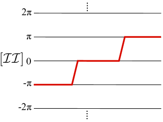
Figure 1: A schematic figure of an example of two instanton configurations $[\mathcal{I}\mathcal{I}]$. Each horizontal line stands for the vacuum in the sine-Gordon potential.

The amplitude of two instantons shown in Fig. 1 is obtained as

$$[\mathcal{I}\mathcal{I}]e^{-2i\theta}\xi^{-2}\,=\,\int_{0}^{\infty}dR\exp\left(-{2\over{g^{2}}}e^{-R}-\epsilon R\right) \,=\,\left({g^{2}\over{2}}\right)^{\epsilon}\int_{0}^{2/g^{2}}ds\,e^{-s}s^{\epsilon-1}$$

$$\,\overset{|g^{2}|\ll 1}{\longrightarrow}\,\left({g^{2}\over{2}}\right)^{\epsilon}\Gamma(\epsilon)$$

$$\,=\,-\left(\gamma\,+\,\log{2\over{g^{2}}}\right)\,+\,O\left(\frac{1}{\epsilon}\right)\,+\,O(\epsilon)\,,$$ (29)

where $\gamma$ is the Euler constant and $\xi$ is an instanton factor defined by

$$\xi\equiv e^{-S_{I}}/\sqrt{\pi g^{2}}=e^{-1/(2g^{2})}/\sqrt{\pi g^{2}}.$$ (30)

Here we have neglected terms of order $O(g^{2})$ or higher. To simplify the formula, we divide the amplitude by $\xi^{2}$ and $e^{2i\theta}$. Precisely speaking, the interaction energy between instantons at small separation $R\ll 1$ may not be precisely represented by the potential in Eq.(26). However, our result is unchanged as long as $|g^{2}|\ll 1$ is satisfied. We need to subtract the divergent term $O(1/\epsilon)$ while the $O(\epsilon)$ term disappears in the $\epsilon\to 0$ limit. The contribution from this amplitude to the energy eigenvalue of the lowest band is then given by

$$\triangle E^{(2,0)}\,=\,e^{2i\theta}\xi^{2}\,\left(\gamma\,+\,\log{2\over{g^{2}}}\right)\,,$$ (31)

where the superscript $(2,0)$ stands for two-instanton and zero–anti-instanton amplitude. We note that the contribution from the two anti-instanton amplitude is obtained by replacing $e^{2i\theta}$ by $e^{-2i\theta}$.

III.3 1 instanton $+$ 1 anti-instanton

The amplitude of one instanton and one anti-instanton amplitude is composed of two configurations $[\mathcal{I}\bar{\mathcal{I}}]$ and $[\bar{\mathcal{I}}\mathcal{I}]$, as shown in Fig. 2. In these cases, the interaction between the two constituents is attractive, and the quasi moduli integral is ill-defined. Therefore we introduce the Bogomolnyi–Zinn-Justin (BZJ) prescription Bogomolny:1980ur ; ZinnJustin:1981dx : we first evaluate the integral by taking $-g^{2}>0$, and then we analytically continue the result from $-g^{2}>0$ back to $g^{2}>0$ in the complex $g^{2}$ plane. This procedure provides the imaginary ambiguity depending on the path of the analytic continuation as $-g^{2}=e^{\mp i\pi}g^{2}$.

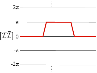
Figure 2: A schematic figure of an example of one-instanton and one anti-instanton amplitude ($[\mathcal{I}\bar{\mathcal{I}}],[\bar{\mathcal{I}}\mathcal{I}]$). Each horizontal line stands for the vacuum in the sine-Gordon potential.

The amplitude of one-instanton and one anti-instanton configuration $[\mathcal{I}\bar{\mathcal{I}}]$ corresponding to the left of Fig. 2 is obtained as

$$[\mathcal{I}\bar{\mathcal{I}}]\xi^{-2} \,=\,\int_{0}^{\infty}dR\,\exp\left(-{2\over{-g^{2}}}e^{-R}-\epsilon R\right)\overset{|g^{2}|\ll 1}{\longrightarrow}\,\left({-g^{2}\over{2}}\right)^{\epsilon}\Gamma(\epsilon)$$

$$\,\overset{-g^{2}=e^{\mp i\pi}g^{2}}{\longrightarrow}\,-\left(\gamma\,+\,\log{2\over{e^{\mp i\pi}g^{2}}}\right)\,+\,O\left(\frac{1}{\epsilon}\right)\,+\,O(\epsilon)$$

$$\,=\,-\left(\gamma\,+\,\log{2\over{g^{2}}}\right)\mp i\pi\,+\,O\left(\frac{1}{\epsilon}\right)\,+\,O(\epsilon)\,,$$ (32)

where we perform the integral in the first line by considering $-g^{2}>0$, and in the second line analytically continue $-g^{2}>0$ back to $g^{2}>0$ in the complex $g^{2}$ plane Bogomolny:1980ur ; ZinnJustin:1981dx . The third line shows a two-fold ambiguous expression of $-g^{2}$ depending on the path of analytic continuation as $-g^{2}=e^{\mp i\pi}g^{2}$. As with the two-instanton case, we have subtracted the divergent part $O(1/\epsilon)$ while the $O(\epsilon)$ term disappears in the $\epsilon\to 0$ limit.

Another amplitude of one-instanton and one anti-instanton configurations $[\bar{\mathcal{I}}\mathcal{I}]$ corresponding to the right of Fig. 2 turns out to give identical contribution as that in Eq.(32). The total contribution is given by the sum of them with dropping $O(1/\epsilon)$ and $O(\epsilon)$ terms,

$$([\mathcal{I}\bar{\mathcal{I}}]\,+\,[\bar{\mathcal{I}}\mathcal{I}])\xi^{-2}\,=\,-2\left(\gamma\,+\,\log{2\over{g^{2}}}\right)\,\mp\,2i\pi\,.$$ (33)

Its contribution to the energy eigenvalue of the lowest band is then given by

$$\triangle E^{(1,1)}\,=\,\xi^{2}\,\left[2\left(\gamma\,+\,\log{2\over{g^{2}}}\right)\,\pm\,2i\pi\right]\,.$$ (34)

If the resurgence idea is valid, this imaginary ambiguity should cancel the imaginary ambiguity of the non-Borel summable divergent series of the perturbative contribution.

$${\rm Im}[\triangle E^{(1,1)}]+{\rm Im}[E_{\rm pert}]=0.$$ (35)

If we insert Eqs.(34) and (35) into the dispersion relation in Eq.(9), we should be able to reproduce the large-order behavior of the perturbation series

$$a_{k} ={-1\over{\pi}}\int_{0}^{\infty}\,dg^{2}\,{{\rm Im}[E_{\rm pert}(g^{2})]\over{(g^{2})^{k+1}}}\,=\,{1\over{\pi}}\int_{0}^{\infty}\,dg^{2}\,{{\rm Im}[\triangle E^{(1,1)}]\over{(g^{2})^{k+1}}}$$

$$\,=\,-{1\over{\pi}}\int_{0}^{\infty}\,d(g^{2})\,{2e^{-1/g^{2}}\over{(g^{2})^{k+2}}}\,=\,-{2\over{\pi}}\,k!\,\quad\quad\quad\quad\quad\,(k\geq 2)\,,$$ (36)

in accordance with the leading large-order behavior of the perturbation series ZinnJustin:1981dx . Thus we find that the imaginary ambiguity of the instanton–anti-instanton amplitude correctly cancels the imaginary ambiguity of the Borel resummation of the (non-Borel summable) perturbation series.

III.4 3 instantons

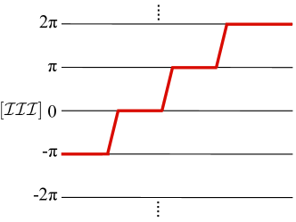
Figure 3: A schematic figure of an example of three-instanton amplitudes ($[\mathcal{I}\mathcal{I}\mathcal{I}]$). Each horizontal line stands for the vacuum in the sine-Gordon potential.

For the three-instanton amplitude shown in Fig. 3, we have two quasi modulus $R_{1},R_{2}$ corresponding to the separations between adjacent instantons. For multiple moduli integral of each given configuration, we need to specify subtraction scheme explicitly, and propose the following:

1. Enumerate possible ordering of quasi moduli integrations, such as $\int dR_{1}\int dR_{2}$ and $\int dR_{2}\int dR_{1}$ for the three instanton case.

2. Subtract possible poles like $1/\epsilon$ for the first integration, and then perform the next integration successively, and retain the finite piece.

3. Average the results of all possible orderings.

Incorporating the repulsive potentials between adjacent instantons, we obtain the three instanton amplitude as

$$[\mathcal{I}\mathcal{I}\mathcal{I}]e^{-3i\theta}\xi^{-3} \,=\,\int_{0}^{\infty}dR_{1}\int_{0}^{\infty}dR_{2}\exp\left[-{2\over{g^{2}}}(e^{-R_{1}}+e^{-R_{2}})-\epsilon(R_{1}+R_{2})\right]$$

$$\,\overset{|g^{2}|\ll 1}{\longrightarrow}\,\left({g^{2}\over{2}}\right)^{\epsilon}\Gamma(\epsilon)\left[\left({g^{2}\over{2}}\right)^{\epsilon}\Gamma(\epsilon)-{1\over{\epsilon}}\right]$$

$$\,=\,{3\over{2}}\left(\gamma+\log{2\over{g^{2}}}\right)^{2}\,+\,{\pi^{2}\over{12}}\,+\,O\left(\frac{1}{\epsilon}\right)\,+\,O(\epsilon)\,.$$ (37)

In the three instanton case, we have two possible orderings of the multi integral, each of which gives the identical contribution. Then the three instanton contribution to the energy eigenvalue of the lowest band is given by

$$\triangle E^{(3,0)}\,=\,-e^{3i\theta}\,\xi^{3}\,\left[{3\over{2}}\left(\gamma+\log{2\over{g^{2}}}\right)^{2}\,+\,{\pi^{2}\over{12}}\right]\,.$$ (38)

We note that the contribution from the three anti-instanton amplitude is obtained by replacing $e^{3i\theta}$ by $e^{-3i\theta}$.

III.5 2 instantons $+$ 1 anti-instanton

The two-instanton and one–anti-instanton amplitudes consist of three types of configurations, as shown in Fig. 4.

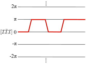
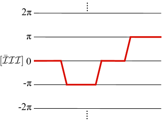
Figure 4: A schematic figure of an example of two-instanton and one–anti-instanton amplitudes ($[\mathcal{I}\bar{\mathcal{I}}\mathcal{I}],[\mathcal{I}\mathcal{I}\bar{\mathcal{I}}],[\bar{\mathcal{I}}\mathcal{I}\mathcal{I}]$). Each horizontal line stands for the vacuum in the sine-Gordon potential.

The first one is $[\mathcal{I}\bar{\mathcal{I}}\mathcal{I}]$, where the anti-instanton is sandwiched between two instantons. For this type of configuration, adjacent constituent (anti-)instantons attract each other. Therefore we first take $-g^{2}>0$ in order to apply the BZJ prescription to the integral, and follow our subtraction prescription

$$[\mathcal{I}\bar{\mathcal{I}}\mathcal{I}]e^{-i\theta}\xi^{-3} \,=\,\int_{0}^{\infty}dR_{1}dR_{2}\exp\left[-{2\over{-g^{2}}}(e^{-R_{1}}+e^{-R_{2}})-\epsilon(R_{1}+R_{2})\right]$$

$$\,\overset{|g^{2}|\ll 1}{\longrightarrow}\,\left({-g^{2}\over{2}}\right)^{\epsilon}\Gamma(\epsilon)\left[\left({-g^{2}\over{2}}\right)^{\epsilon}\Gamma(\epsilon)-{1\over{\epsilon}}\right]$$

$$\,\overset{-g^{2}=g^{2}e^{\mp i\pi}}{\longrightarrow}\,{3\over{2}}\left(\gamma+\log{2\over{g^{2}}}\right)^{2}\,-\,{17\pi^{2}\over{12}}\pm 3i\pi\left(\gamma+\log{2\over{g^{2}}}\right)\,+\,O\left(\frac{1}{\epsilon}\right)\,+\,O(\epsilon)\,,$$ (39)

where we again subtract $1/\epsilon$ in the first integral, before integrating the second quasi-moduli.

The second type of configuration is $[\mathcal{I}\mathcal{I}\bar{\mathcal{I}}]$, where one pair of constituents is repulsive and the other attractive. In order to apply the BZJ prescription only to the attractive part of the interaction, we temporarily distinguish two coupling constants $g^{2}$ for the repulsive interaction and $\tilde{g}^{2}$ for the attractive interaction, and apply the BZJ prescription to $\tilde{g}^{2}$, but not to $g^{2}$. After analytic continuation, we identify $\tilde{g}^{2}$ as the original $g^{2}$ at the end of the calculation. The moduli-integral of $[\mathcal{I}\mathcal{I}\bar{\mathcal{I}}]$ is given by

$$[\mathcal{I}\mathcal{I}\bar{\mathcal{I}}]e^{-i\theta}\xi^{-3}\,=\,\int_{0}^{\infty}dR_{1}dR_{2}\,\exp\left[-{2\over{g^{2}}}e^{-R_{1}}-{2\over{-\tilde{g}^{2}}}e^{-R_{2}}-\epsilon(R_{1}+R_{2})\right]\,.$$ (40)

For this configuration $[\mathcal{I}\mathcal{I}\bar{\mathcal{I}}]$, we have two possible orderings of moduli integral. The first ordering is to integrate over $R_{2}$ and to subtract the $1/\epsilon$ pole, before integrating over $R_{1}$. We call this ordering as $F_{1}(g^{2})$

$$F_{1}(g^{2}) \,\overset{|g^{2}|,|\tilde{g}^{2}|\ll 1}{\longrightarrow}\,\left({g^{2}\over{2}}\right)^{\epsilon}\Gamma(\epsilon)\left[\left({-\tilde{g}^{2}\over{2}}\right)^{\epsilon}\Gamma(\epsilon)-{1\over{\epsilon}}\right]$$

$$\,\overset{-\tilde{g}^{2}=\tilde{g}^{2}e^{\mp i\pi}}{\longrightarrow}\,{3\over{2}}\left(\gamma+\log{2\over{g^{2}}}\right)^{2}\,-\,{5\pi^{2}\over{12}}\pm 2i\pi\left(\gamma+\log{2\over{g^{2}}}\right)\,+\,O\left(\frac{1}{\epsilon}\right)+O(\epsilon)\,.$$ (41)

We call the result of another ordering as $F_{2}(g^{2})$, which is given by integrating over $R_{1}$ first and then over $R_{2}$

$$F_{2}(g^{2}) \,\overset{|g^{2}|,|\tilde{g}^{2}|\ll 1}{\longrightarrow}\,\left({-\tilde{g}^{2}\over{2}}\right)^{\epsilon}\Gamma(\epsilon)\left[\left({g^{2}\over{2}}\right)^{\epsilon}\Gamma(\epsilon)-{1\over{\epsilon}}\right]$$

$$\,\overset{-\tilde{g}^{2}=\tilde{g}^{2}e^{\mp i\pi}}{\longrightarrow}\,{3\over{2}}\left(\gamma+\log{2\over{g^{2}}}\right)^{2}\,+\,{\pi^{2}\over{12}}\pm i\pi\left(\gamma+\log{2\over{g^{2}}}\right)\,+\,O\left(\frac{1}{\epsilon}\right)\,+\,O(\epsilon).$$ (42)

In the final expressions for $F_{1},F_{2}$, we implicitly put back $\tilde{g}^{2}$ to $g^{2}$ after analytic continuation. We obtain the amplitude of $[\mathcal{I}\mathcal{I}\bar{\mathcal{I}}]$ as an average of $F_{1}(g^{2})$ and $F_{2}(g^{2})$ with dropping $O(1/\epsilon)$ and $O(\epsilon)$ terms

$$[\mathcal{I}\mathcal{I}\bar{\mathcal{I}}]e^{-i\theta}\xi^{-3} \,=\,(F_{1}\,+\,F_{2})/2$$

$$\,=\,{3\over{2}}\left(\gamma+\log{2\over{g^{2}}}\right)^{2}\,-\,{\pi^{2}\over{6}}\pm{3\over{2}}i\pi\left(\gamma+\log{2\over{g^{2}}}\right)\,.$$ (43)

The third type of configuration is $[\bar{\mathcal{I}}\mathcal{I}\mathcal{I}]$, which gives the identical result as the second type in Eq.(43) : $[\bar{\mathcal{I}}\mathcal{I}\mathcal{I}]=[\mathcal{I}\mathcal{I}\bar{\mathcal{I}}]$.

By taking the sum of all three types of configurations, we end up with

$$([\mathcal{I}\bar{\mathcal{I}}\mathcal{I}]\,+\,[\mathcal{I}\mathcal{I}\bar{\mathcal{I}}]\,+\,[\bar{\mathcal{I}}\mathcal{I}\mathcal{I}])e^{-i\theta}\xi^{-3}\,=\,{9\over{2}}\left[\left(\gamma+\log{2\over{g^{2}}}\right)^{2}\,-\,{7\pi^{2}\over{18}}\pm{4\over{3}}i\pi\left(\gamma+\log{2\over{g^{2}}}\right)\right]\,.$$ (44)

Its contribution to the energy eigenvalue of the lowest band is then given by

$$\triangle E^{(2,1)}\,=\,-{9\over{2}}e^{i\theta}\,\xi^{3}\left[\left(\gamma+\log{2\over{g^{2}}}\right)^{2}\,-\,{7\pi^{2}\over{18}}\pm{4\over{3}}i\pi\left(\gamma+\log{2\over{g^{2}}}\right)\right]\,.$$ (45)

We note that the two–anti-instanton and one-instanton contribution is obtained by replacing $e^{i\theta}$ by $e^{-i\theta}$.

Resurgence implies that the two–anti-instanton and one-instanton amplitude should correspond to the large-order behavior of the perturbation series around the one-instanton saddle point. Using the cancellation between imaginary ambiguities of Borel resummed perturbation series around one-instanton saddle point and of the two–anti-instanton and one-instanton amplitude, the large-order behavior of the perturbation series around the one instanton saddle point can be estimated from the imaginary part of (45) by means of the dispersion relation as

$$a_{k} \,\approx\,{1\over{\pi}}\int_{0}^{\infty}\,dg^{2}\,{{\rm Im}[\triangle E^{(2,1)}e^{-i\theta}/\xi]\over{(g^{2})^{k+1}}}\,=\,{6\over{\pi}}\int_{0}^{\infty}\,dg^{2}\,{e^{-1/g^{2}}(\gamma+\log(2/g^{2}))\over{(g^{2})^{k+2}}}$$

$$\,=\,{6\over{\pi}}k!\,\left(\log 2\,+\,{s(k+1,2)\over{k!}}\right)\quad\quad\quad\quad\quad\,(k\geq 2)\,,$$ (46)

where $s(k+1,2)$ is the Stirling number of the first kind, which is the solution of the recurrence relation $s(k+1,2)=(k+1)s(k,2)+k!$. The first few numbers are given as $s(k+1,2)=3,11,50,274,1764,13068,109584$ for $k=2,3,4,5,6,7,8$. In Ref. ZinnJustin:1981dx , the large-order perturbative series around one instanton is numerically calculated as

$$a_{k}^{\rm pert.}\,=\,{6\over{\pi}}k!\,\left(\gamma\,+\,\log 2k\right)\,+\,O\left({\log k\over{k}}\right)\,,$$ (47)

which is consistent with Eq. (46) for large $k$.

III.6 4 instantons

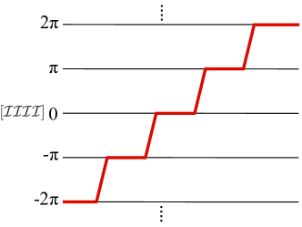
Figure 5: A schematic figure of an example of the four-instanton amplitude $[\mathcal{I}\mathcal{I}\mathcal{I}\mathcal{I}]$. Each horizontal line stands for the vacuum in the sine-Gordon potential.

For the four-instanton amplitude, the interaction between each pair of instantons is repulsive, as shown in Fig. 5. Since all the possible orderings of multi-moduli integral has the identical contribution, we easily obtain the amplitude using the polygamma function defined as $\psi^{(2)}(z)\equiv d^{3}\log\Gamma(z)/dz^{3}$

$$[\mathcal{I}\mathcal{I}\mathcal{I}\mathcal{I}]e^{-4i\theta}\xi^{-4} \,=\,\int_{0}^{\infty}dR_{1}dR_{2}dR_{3}\,\exp\left[-{2\over{g^{2}}}(e^{-R_{1}}+e^{-R_{2}}+e^{-R_{3}})-\epsilon(R_{1}+R_{2}+R_{3})\right]$$

$$\,\overset{|g^{2}|\ll 1}{\longrightarrow}\,\left({g^{2}\over{2}}\right)^{\epsilon}\Gamma(\epsilon)\left[\left({g^{2}\over{2}}\right)^{\epsilon}\Gamma(\epsilon)\left\{\left({g^{2}\over{2}}\right)^{\epsilon}\Gamma(\epsilon)-{1\over{\epsilon}}\right\}+{\gamma+\log(2/g^{2})\over{\epsilon}}\right]$$

$$\,=\,-{8\over{3}}\left[\left(\gamma+\log{2\over{g^{2}}}\right)^{3}\,+\,{\pi^{2}\over{8}}\left(\gamma+\log{2\over{g^{2}}}\right)-{1\over{16}}\psi^{(2)}(1)\right]\,+\,O\left(\frac{1}{\epsilon}\right)\,+\,O(\epsilon)\,,$$ (48)

where we have first subtracted $1/\epsilon$ in the first integral $dR_{3}$, and subtracted $-(\gamma+\log(2/g^{2}))/\epsilon$ in the next integral $dR_{2}$, and finally dropped the $O(1/\epsilon)$ term in the integral $dR_{1}$. Its contribution to the eigenvalue of the lowest band is then given by

$$\triangle E^{(4,0)}\,=\,{8\over{3}}e^{4i\theta}\,\xi^{4}\left[\left(\gamma+\log{2\over{g^{2}}}\right)^{3}\,+\,{\pi^{2}\over{8}}\left(\gamma+\log{2\over{g^{2}}}\right)-{1\over{16}}\psi^{(2)}(1)\right]\,.$$ (49)

The four anti-instanton contribution is obtained by replacing $e^{4i\theta}$ by $e^{-4i\theta}$.

III.7 3 instantons $+$ 1 anti-instanton

The three-instanton and one–anti-instanton amplitudes consist of four types of configurations $[\mathcal{I}\mathcal{I}\mathcal{I}\bar{\mathcal{I}}]$, $[\bar{\mathcal{I}}\mathcal{I}\mathcal{I}\mathcal{I}]$, $[\mathcal{I}\bar{\mathcal{I}}\mathcal{I}\mathcal{I}]$ and $[\mathcal{I}\mathcal{I}\bar{\mathcal{I}}\mathcal{I}]$, as shown in Fig. 6.

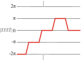
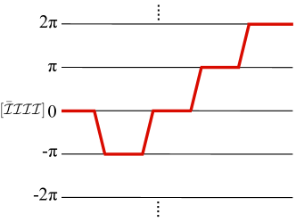
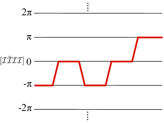
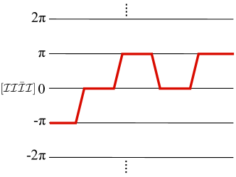
Figure 6: A schematic figure of examples of four-instanton amplitudes ($[\mathcal{I}\mathcal{I}\mathcal{I}\bar{\mathcal{I}}]$, $[\bar{\mathcal{I}}\mathcal{I}\mathcal{I}\mathcal{I}]$, $[\mathcal{I}\bar{\mathcal{I}}\mathcal{I}\mathcal{I}]$ and $[\mathcal{I}\mathcal{I}\bar{\mathcal{I}}\mathcal{I}]$). Each horizontal line stands for the vacuum in the sine-Gordon potential.

In the first configuration $[\mathcal{I}\mathcal{I}\mathcal{I}\bar{\mathcal{I}}]$, two pairs of adjacent instantons have repulsive interactions, and the other is attractive. We again apply the BZJ prescription only to the integral for the pair with the attractive interaction, where we denote the coupling as $\tilde{g}^{2}$, evaluate the integral at $-\tilde{g}^{2}>0$, and analytically continue to $\tilde{g}^{2}>0$, while keeping $g^{2}>0$ for the repulsive interactions. The multi-moduli integral is given by

$${[\mathcal{I}\mathcal{I}\mathcal{I}\bar{\mathcal{I}}]\over{e^{2i\theta}\xi^{4}}}\,=\,\int_{0}^{\infty}dR_{1}dR_{2}dR_{3}\,\exp\left[-{2\over{g^{2}}}e^{-R_{1}}-{2\over{g^{2}}}e^{-R_{2}}-{2\over{-\tilde{g}^{2}}}e^{-R_{3}}-\epsilon(R_{1}+R_{2}+R_{3})\right]\,.$$ (50)

Here we have three orderings of the multi-integral, distinguished by the ordering of $dR_{3}$ (attractive interaction) relative to $dR_{1},dR_{2}$. We denote the results $G_{1}(g^{2})$, $G_{2}(g^{2})$, and $G_{3}(g^{2})$ as the first, the second, and the third integral, respectively. Referring the calculations given in Appendix A, we just show the result

$$G_{1}(g^{2}) \,=\,-{8\over{3}}\left(\gamma+\log{2\over{g^{2}}}\right)^{3}\,+\,{7\over{6}}\pi^{2}\left(\gamma+\log{2\over{g^{2}}}\right)+{1\over{6}}\psi^{(2)}(1)\,\mp\,4i\pi\left(\gamma+\log{2\over{g^{2}}}\right)^{2}\,,$$

$$G_{2}(g^{2}) \,=\,-{8\over{3}}\left(\gamma+\log{2\over{g^{2}}}\right)^{3}\,+\,{1\over{6}}\pi^{2}\left(\gamma+\log{2\over{g^{2}}}\right)+{1\over{6}}\psi^{(2)}(1)\,\mp\,i\pi\Big{[}{5\over{2}}\left(\gamma+\log{2\over{g^{2}}}\right)^{2}+{\pi^{2}\over{12}}\Big{]}\,,$$

$$G_{3}(g^{2}) \,=\,-{8\over{3}}\left(\gamma+\log{2\over{g^{2}}}\right)^{3}\,-\,{1\over{3}}\pi^{2}\left(\gamma+\log{2\over{g^{2}}}\right)+{1\over{6}}\psi^{(2)}(1)\,\mp\,i\pi\Big{[}{3\over{2}}\left(\gamma+\log{2\over{g^{2}}}\right)^{2}+{\pi^{2}\over{12}}\Big{]}\,.$$ (51)

We obtain the amplitude of $[\mathcal{I}\mathcal{I}\mathcal{I}\bar{\mathcal{I}}]$ as the average of $G_{1}(g^{2})$, $G_{2}(g^{2})$ and $G_{3}(g^{2})$,

$${[\mathcal{I}\mathcal{I}\mathcal{I}\bar{\mathcal{I}}]\over{e^{2i\theta}\xi^{4}}} \,=\,(G_{1}(g^{2})\,+\,G_{2}(g^{2})\,+\,G_{3}(g^{2}))/3$$

$$\,=\,-{8\over{3}}\left(\gamma+\log{2\over{g^{2}}}\right)^{3}\,+\,{1\over{3}}\pi^{2}\left(\gamma+\log{2\over{g^{2}}}\right)+{1\over{6}}\psi^{(2)}(1)\,\mp\,i\pi\Big{[}{8\over{3}}\left(\gamma+\log{2\over{g^{2}}}\right)^{2}+{\pi^{2}\over{18}}\Big{]}\,.$$ (52)

The amplitude of the second configuration $[\bar{\mathcal{I}}\mathcal{I}\mathcal{I}\mathcal{I}]$ is found to give identical result as the above configuration : $[\bar{\mathcal{I}}\mathcal{I}\mathcal{I}\mathcal{I}]=[\mathcal{I}\mathcal{I}\mathcal{I}\bar{\mathcal{I}}]$.

In the third configuration $[\mathcal{I}\bar{\mathcal{I}}\mathcal{I}\mathcal{I}]$, the two pairs of adjacent instantons have attractive interactions, while the other is repulsive. We again apply the BZJ prescription only to the attractive pairs, by denoting the couplings as $\tilde{g}^{2}$. The multi-integral is given as

$${[\mathcal{I}\bar{\mathcal{I}}\mathcal{I}\mathcal{I}]\over{e^{2i\theta}\xi^{4}}}\,=\,\int_{0}^{\infty}dR_{1}dR_{2}dR_{3}\,\exp\left[-{2\over{g^{2}}}e^{-R_{1}}-{2\over{-\tilde{g}^{2}}}e^{-R_{2}}-{2\over{-\tilde{g}^{2}}}e^{-R_{3}}-\epsilon(R_{1}+R_{2}+R_{3})\right]\,.$$ (53)

We have three orderings of the multi-integral, distinguished by the ordering of $dR_{1}$ (repulsive interaction) relative to $dR_{2},dR_{3}$. We denote the results $G_{4}(g^{2})$, $G_{5}(g^{2})$, and $G_{6}(g^{2})$ as the first, the second, and the third integral, respectively. Referring the calculations given in Appendix A, we just show the result

$$G_{4} \,=\,-{8\over{3}}\left(\gamma+\log{2\over{g^{2}}}\right)^{3}\,+\,{7\over{6}}\pi^{2}\left(\gamma+\log{2\over{g^{2}}}\right)+{1\over{6}}\psi^{(2)}(1)\,\mp\,i\pi\Big{[}4\left(\gamma+\log{2\over{g^{2}}}\right)^{2}+{\pi^{2}\over{6}}\Big{]}\,,$$

$$G_{5} \,=\,-{8\over{3}}\left(\gamma+\log{2\over{g^{2}}}\right)^{3}\,+\,{19\over{6}}\pi^{2}\left(\gamma+\log{2\over{g^{2}}}\right)+{1\over{6}}\psi^{(2)}(1)\,\mp\,i\pi\Big{[}{11\over{2}}\left(\gamma+\log{2\over{g^{2}}}\right)^{2}-{5\pi^{2}\over{12}}\Big{]}\,,$$

$$G_{6} \,=\,-{8\over{3}}\left(\gamma+\log{2\over{g^{2}}}\right)^{3}\,+\,{14\over{3}}\pi^{2}\left(\gamma+\log{2\over{g^{2}}}\right)+{1\over{6}}\psi^{(2)}(1)\,\mp\,i\pi\Big{[}{13\over{2}}\left(\gamma+\log{2\over{g^{2}}}\right)^{2}-{11\pi^{2}\over{12}}\Big{]}\,.$$ (54)

We obtain the amplitude of $[\mathcal{I}\bar{\mathcal{I}}\mathcal{I}\mathcal{I}]$ as the average of $G_{4}(g^{2})$, $G_{5}(g^{2})$ and $G_{6}(g^{2})$,

$${[\mathcal{I}\bar{\mathcal{I}}\mathcal{I}\mathcal{I}]\over{e^{2i\theta}\xi^{4}}} \,=\,(G_{4}(g^{2})\,+\,G_{5}(g^{2})\,+\,G_{6}(g^{2}))/3$$

$$\,=\,-{8\over{3}}\left(\gamma+\log{2\over{g^{2}}}\right)^{3}\,+\,3\pi^{2}\left(\gamma+\log{2\over{g^{2}}}\right)+{1\over{6}}\psi^{(2)}(1)\,\mp\,i\pi\Big{[}{16\over{3}}\left(\gamma+\log{2\over{g^{2}}}\right)^{2}-{7\pi^{2}\over{18}}\Big{]}\,.$$ (55)

The amplitude of the fourth configuration $[\mathcal{I}\mathcal{I}\bar{\mathcal{I}}\mathcal{I}]$ turns out to be identical to the above third configuration : $[\mathcal{I}\mathcal{I}\bar{\mathcal{I}}\mathcal{I}]=[\mathcal{I}\bar{\mathcal{I}}\mathcal{I}\mathcal{I}]$.

The sum of all the four configurations gives

$$([\mathcal{I}\mathcal{I}\mathcal{I}\bar{\mathcal{I}}]+[\bar{\mathcal{I}}\mathcal{I}\mathcal{I}\mathcal{I}]+[\mathcal{I}\bar{\mathcal{I}}\mathcal{I}\mathcal{I}]+[\mathcal{I}\mathcal{I}\bar{\mathcal{I}}\mathcal{I}])e^{-2i\theta}\xi^{-4}$$

$$\,=\,-{32\over{3}}\left(\gamma+\log{2\over{g^{2}}}\right)^{3}\,+\,{20\over{3}}\pi^{2}\left(\gamma+\log{2\over{g^{2}}}\right)+{2\over{3}}\psi^{(2)}(1)\,\mp\,i\pi\Big{[}16\left(\gamma+\log{2\over{g^{2}}}\right)^{2}-{2\pi^{2}\over{3}}\Big{]}\,.$$ (56)

Therefore the contribution of three instantons and one anti-instanton to the energy eigenvalue of the lowest band is given by

$$\triangle E^{(3,1)}$$

$$\,=\,e^{2i\theta}\,\xi^{4}\left[{32\over{3}}\left(\gamma+\log{2\over{g^{2}}}\right)^{3}\,-\,{20\over{3}}\pi^{2}\left(\gamma+\log{2\over{g^{2}}}\right)-{2\over{3}}\psi^{(2)}(1)\,\pm\,i\pi\Big{[}16\left(\gamma+\log{2\over{g^{2}}}\right)^{2}-{2\pi^{2}\over{3}}\Big{]}\right]\,.$$ (57)

We note that the three anti-instanton and one-instanton contribution is obtained by replacing $e^{2i\theta}$ by $e^{-2i\theta}$.

Resurgence implies that the three-instanton and one–anti-instanton amplitude should correspond to the large-order behavior of the perturbation series around the two-instanton saddle point. Using the cancellation between imaginary ambiguities of Borel resummed perturbation series around two-instanton saddle point and of the three-instanton and one–anti-instanton amplitude, the large-order behavior of the perturbation series around the two instanton saddle point can be estimated from the imaginary part of (57) by means of the dispersion relation as

$$a_{k} \,\approx\,{1\over{\pi}}\int_{0}^{\infty}\,dg^{2}\,{{\rm Im}[\triangle E^{(3,1)}e^{-2i\theta}/\xi^{2}]\over{(g^{2})^{k+1}}}$$

$$\,=\,-{16\over{\pi}}\int_{0}^{\infty}\,dg^{2}\,{e^{-1/g^{2}}\over{(g^{2})^{k+2}}}\left((\gamma+\log 2)^{2}-{\pi^{2}\over{24}}\,-\,2(\gamma+\log 2)\log(g^{2})\,+\,\log^{2}(g^{2})\right)\,.$$ (58)

This integral can be performed numerically, and the first few results are $a_{k}\,\sim\,-48.826,\,-191.16,\,-919.05,\,-5273.0$ for $k=2,3,4,5$. One should be able to check this large-order behavior, by performing the perturbation around the two-instanton saddle point to high orders.

III.8 2 instantons $+$ 2 anti-instantons

The two-instanton and two-anti-instanton amplitudes consist of six types of configurations $[\mathcal{I}\bar{\mathcal{I}}\mathcal{I}\bar{\mathcal{I}}]$, $[\bar{\mathcal{I}}\mathcal{I}\bar{\mathcal{I}}\mathcal{I}]$, $[\mathcal{I}\mathcal{I}\bar{\mathcal{I}}\bar{\mathcal{I}}]$, $[\bar{\mathcal{I}}\bar{\mathcal{I}}\mathcal{I}\mathcal{I}]$, $[\mathcal{I}\bar{\mathcal{I}}\bar{\mathcal{I}}\mathcal{I}]$ and $[\bar{\mathcal{I}}\mathcal{I}\mathcal{I}\bar{\mathcal{I}}]$, as shown in Fig. 7.

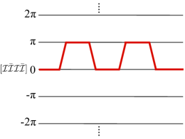
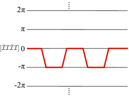
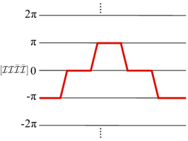
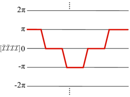
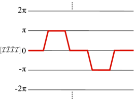
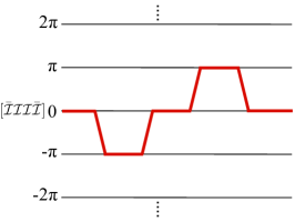
Figure 7: A schematic figure of examples of four-instanton amplitudes ($[\mathcal{I}\bar{\mathcal{I}}\mathcal{I}\bar{\mathcal{I}}]$, $[\bar{\mathcal{I}}\mathcal{I}\bar{\mathcal{I}}\mathcal{I}]$, $[\mathcal{I}\mathcal{I}\bar{\mathcal{I}}\bar{\mathcal{I}}]$, $[\bar{\mathcal{I}}\bar{\mathcal{I}}\mathcal{I}\mathcal{I}]$, $[\mathcal{I}\bar{\mathcal{I}}\bar{\mathcal{I}}\mathcal{I}]$ and $[\bar{\mathcal{I}}\mathcal{I}\mathcal{I}\bar{\mathcal{I}}]$). Each horizontal line stands for the vacuum in the sine-Gordon potential.

The first one is $[\mathcal{I}\bar{\mathcal{I}}\mathcal{I}\bar{\mathcal{I}}]$, where all three adjacent pairs of constituents have attractive interactions. Thus we apply the simple BZJ prescription to all the integration. Since all the orderings of the multi integral have the same contributions, the amplitude can be easily calculated as

$$[\mathcal{I}\bar{\mathcal{I}}\mathcal{I}\bar{\mathcal{I}}]\xi^{-4} \,=\,\int_{0}^{\infty}dR_{1}dR_{2}dR_{3}\exp\left[-{2\over{-g^{2}}}(e^{-R_{1}}+e^{-R_{2}}+e^{-R_{3}})-\epsilon(R_{1}+R_{2}+R_{3})\right]$$

$$\,\overset{|g^{2}|\ll 1}{\longrightarrow}\,\left({-g^{2}\over{2}}\right)^{\epsilon}\Gamma(\epsilon)\left[\left({-g^{2}\over{2}}\right)^{\epsilon}\Gamma(\epsilon)\left\{\left({-g^{2}\over{2}}\right)^{\epsilon}\Gamma(\epsilon)-{1\over{\epsilon}}\right\}+{\gamma+\log(2/g^{2})\over{\epsilon}}\right]$$

$$\,\overset{-g^{2}\to g^{2}e^{\mp i\pi}}{\longrightarrow}\,-{8\over{3}}\left(\gamma+\log{2\over{g^{2}}}\right)^{3}\,+\,{23\over{3}}\pi^{2}\left(\gamma+\log{2\over{g^{2}}}\right)+{1\over{6}}\psi^{(2)}(1)$$

$$\qquad\qquad\qquad\mp\,i\pi\Big{[}8\left(\gamma+\log{2\over{g^{2}}}\right)^{2}-{7\pi^{2}\over{3}}\Big{]}\,+\,O\left(\frac{1}{\epsilon}\right)\,+\,O(\epsilon)\,.$$ (59)

The second configuration $[\bar{\mathcal{I}}\mathcal{I}\bar{\mathcal{I}}\mathcal{I}]$ gives identical result as the first one : $[\bar{\mathcal{I}}\mathcal{I}\bar{\mathcal{I}}\mathcal{I}]=[\mathcal{I}\bar{\mathcal{I}}\mathcal{I}\bar{\mathcal{I}}]$.

For the third $[\mathcal{I}\mathcal{I}\bar{\mathcal{I}}\bar{\mathcal{I}}]$ and fourth configurations $[\bar{\mathcal{I}}\bar{\mathcal{I}}\mathcal{I}\mathcal{I}]$, the two pairs of interactions are repulsive, but the other pair is attractive. Since these moduli-integrals are the same as that of $[\mathcal{I}\mathcal{I}\mathcal{I}\bar{\mathcal{I}}]$ in Eq.(52), we obtain

$$[\mathcal{I}\mathcal{I}\bar{\mathcal{I}}\bar{\mathcal{I}}]\xi^{-4}=[\bar{\mathcal{I}}\bar{\mathcal{I}}\mathcal{I}\mathcal{I}]\xi^{-4}$$

$$\,=\,-{8\over{3}}\left(\gamma+\log{2\over{g^{2}}}\right)^{3}\,+\,{1\over{3}}\pi^{2}\left(\gamma+\log{2\over{g^{2}}}\right)+{1\over{6}}\psi^{(2)}(1)\,\mp\,i\pi\Big{[}{8\over{3}}\left(\gamma+\log{2\over{g^{2}}}\right)^{2}+{\pi^{2}\over{18}}\Big{]}\,.$$ (60)

For the fifth $[\mathcal{I}\bar{\mathcal{I}}\bar{\mathcal{I}}\mathcal{I}]$ and the sixth configurations $[\bar{\mathcal{I}}\mathcal{I}\mathcal{I}\bar{\mathcal{I}}]$, the two pairs of interactions are attractive, but the other pair is repulsive. Since these moduli-integrals are the same as $[\mathcal{I}\bar{\mathcal{I}}\mathcal{I}\mathcal{I}]$ in Eq.(55), we obtain

$$[\mathcal{I}\bar{\mathcal{I}}\bar{\mathcal{I}}\mathcal{I}]\xi^{-4}=[\bar{\mathcal{I}}\mathcal{I}\mathcal{I}\bar{\mathcal{I}}]\xi^{-4}$$

$$\,=\,-{8\over{3}}\left(\gamma+\log{2\over{g^{2}}}\right)^{3}\,+\,3\pi^{2}\left(\gamma+\log{2\over{g^{2}}}\right)+{1\over{6}}\psi^{(2)}(1)\,\mp\,i\pi\Big{[}{16\over{3}}\left(\gamma+\log{2\over{g^{2}}}\right)^{2}-{7\pi^{2}\over{18}}\Big{]}\,.$$ (61)

The sum of all the six configurations gives

$$([\mathcal{I}\bar{\mathcal{I}}\mathcal{I}\bar{\mathcal{I}}]+[\bar{\mathcal{I}}\mathcal{I}\bar{\mathcal{I}}\mathcal{I}]+[\mathcal{I}\mathcal{I}\bar{\mathcal{I}}\bar{\mathcal{I}}]+[\bar{\mathcal{I}}\bar{\mathcal{I}}\mathcal{I}\mathcal{I}]+[\mathcal{I}\bar{\mathcal{I}}\bar{\mathcal{I}}\mathcal{I}]+[\bar{\mathcal{I}}\mathcal{I}\mathcal{I}\bar{\mathcal{I}}])\xi^{-4}$$

$$\,=\, -16\left(\gamma+\log{2\over{g^{2}}}\right)^{3}\,+\,22\pi^{2}\left(\gamma+\log{2\over{g^{2}}}\right)+\psi^{(2)}(1)\,\mp\,i\pi\Big{[}32\left(\gamma+\log{2\over{g^{2}}}\right)^{2}-{16\pi^{2}\over{3}}\Big{]}\,.$$ (62)

Therefore the contribution of two instantons and two anti-instantons to the energy eigenvalue of the lowest band is given by

$$\triangle E^{(2,2)}$$

$$\,=\,\xi^{4}\left[16\left(\gamma+\log{2\over{g^{2}}}\right)^{3}\,-\,22\pi^{2}\left(\gamma+\log{2\over{g^{2}}}\right)-\psi^{(2)}(1)\,\pm\,i\pi\Big{[}32\left(\gamma+\log{2\over{g^{2}}}\right)^{2}-{16\pi^{2}\over{3}}\Big{]}\right]\,.$$ (63)

According to the resurgence, the imaginary part of the two-instanton and two anti-instanton amplitudes should cancel the imaginary part of the Borel resummation of the divergent perturbation series. Using the dispersion relation, we can obtain the large-order behavior of the perturbation series corresponding to the two-instanton and two anti-instanton amplitude in Eq. (63)

$$a_{k} \,\approx\,{1\over{\pi}}\int_{0}^{\infty}\,dg^{2}\,{{\rm Im}[\triangle E^{(2,2)}]\over{(g^{2})^{k+1}}}$$

$$\,=\,-{32\over{\pi^{2}}}\int_{0}^{\infty}\,dg^{2}\,{e^{-2/g^{2}}\over{(g^{2})^{k+3}}}\left((\gamma+\log 2)^{2}-{\pi^{2}\over{6}}\,-\,2(\gamma+\log 2)\log(g^{2})\,+\,\log^{2}(g^{2})\right)\,.$$ (64)

This integral can be performed numerically, and the first few results are $a_{k}\sim-2.4317,\,-7.0925,\,-22.797,\,-82.273$ for $k=2,3,4,5$. Because of the factor $e^{-2/g^{2}}$ associated with the four-instanton action $2/g^{2}=4S_{I}$, the large-order ($k\gg 1$) behavior of $a_{k}$ in Eq. (64) can be estimated with a constant $C$ as

$$a_{k}\,=\,\left({1\over{2}}\right)^{k+2}(k+1)!\,\left[C\,+\,O(\log k/k)\right]\,,$$ (65)

exhibiting the $(1/2)^{k+2}$ factor besides the factorial growth $k!$. This large-order behavior corresponds to the singularity of the Borel transform $B_{\rm pert}(g^{2}t)$ at $t=2/g^{2}=4S_{I}$ in the Borel plane

$$B_{\rm pert}(g^{2}t)\,\approx\,C\sum_{k=0}^{\infty}\left({1\over{2}}\right)^{k+2}\,(k+1)!\,\left({(g^{2}t)^{k}\over{k!}}\right)\,\to\,{C\over{(2-g^{2}t)^{2}}}\,.$$ (66)

This is consistent with the known and expected results in quantum mechanics. We comment that we can also calculate the large-order perturbative behavior around the one-instanton and one–anti-instanton vacuum as $a_{k}\approx{1\over{\pi}}\int_{0}^{\infty}dg^{2}{\rm Im}[\triangle E^{(2,2)}\xi^{-2}]/(g^{2})^{k+1}$.

III.9 General cases: $n$ instantons $+$ $m$ anti-instantons

For general cases with $n$ instantons and $m$ anti-instantons, we have ${}_{(n+m)}C_{n}$ configurations depending on the arrangement of constituents. We can classify these ${}_{(n+m)}C_{n}$ configurations into classes based on how many attractive and repulsive interactions are among the $n+m-1$ nearest-neighbor interactions. (We can classify them into $2\times{\rm min}(n,m)$ classes for $n\not=m$, and $2n-1$ classes for $n=m$ with $n,m\geq 1$.) We use the expression $N_{k,l}$ as the number of configurations including $k$ attractive and $l$ repulsive interactions satisfying $k+l=n+m-1$, and show examples of classification for $(n,m)=(3,2)$, $(n,m)=(3,3)$, $(n,m)=(4,4)$ and $(n,m)=(5,5)$ as following,

$${}_{(3+2)}C_{3}\, = \,N_{4,0}\,+\,N_{3,1}\,+\,N_{2,2}\,+\,N_{1,3}$$

$$= \,1\,+\,4\,+\,3\,+\,2\,,$$ (67)

$${}_{(3+3)}C_{3}\, = \,N_{5,0}\,+\,N_{4,1}\,+\,N_{3,2}\,+\,N_{2,3}\,+\,N_{1,4}$$

$$= \,2\,+\,4\,+\,8\,+\,4\,+\,2\,,$$ (68)

$${}_{(4+4)}C_{4}\, = \,N_{7,0}\,+\,N_{6,1}\,+\,N_{5,2}\,+\,N_{4,3}\,+\,N_{3,4}\,+\,N_{2,5}\,+\,N_{1,6}$$

$$= \,2\,+\,6\,+\,18\,+\,18\,+\,18\,+\,6\,+\,2\,,$$ (69)

$${}_{(5+5)}C_{5}\, = \,N_{9,0}\,+\,N_{8,1}\,+\,N_{7,2}\,+\,N_{6,3}\,+\,N_{5,4}\,+\,N_{4,5}\,+\,N_{3,6}\,+\,N_{2,7}\,+\,N_{1,8}$$

$$= \,2\,+\,8\,+\,32\,+\,48\,+\,72\,+\,48\,+\,32\,+\,8\,+2\,.$$ (70)

When calculating the amplitude of each in the $N_{k,l}$ configurations, we have ${}_{(k+l)}C_{k}$ possible orderings of the multi moduli integrals in relation to the subtraction scheme which is described in Sec. III.1 and III.4. After calculating these ${}_{(k+l)}C_{k}$ integrals, we average the results and obtain a contribution from one of $N_{k,l}$ configurations. As such, we calculate each contribution, and by summing up all the integral results, we end up with the semi-classical amplitude of the configuration with $n$ instantons and $m$ anti-instantons.

IV Comparison to uniform-WKB

IV.1 General formalism

A systematic method called the uniform-WKB method has been applied extensively to study quantum mechanics for potentials with degenerate minima, such as the sine-Gordon quantum mechanics Dunne:2013ada ; Dunne:2014bca . In this method, one combines the ansatz in Eq.(23) with a global boundary condition to take account of the other minima than the one to do perturbative computation. This boundary condition enables one to go beyond the ordinary perturbative computation, and obtain all nonperturbative contributions leading to the resurgence. Defining the even $f_{1}$ and odd $f_{2}$ functions, and the Wronskian $\mathcal{W}$,

$$f_{1}(y)\, =\,{1\over{\sqrt{u^{\prime}(y)}}}\left[D_{\nu}(u(y)/g)\,+\,D_{\nu}(-u(y)/g)\right]\,,$$ (71)

$$f_{2}(y)\, =\,{1\over{\sqrt{u^{\prime}(y)}}}\left[D_{\nu}(u(y)/g)\,-\,D_{\nu}(-u(y)/g)\right]\,,$$ (72)

$$\mathcal{W}\, =\,f_{1}f^{\prime}_{2}-f^{\prime}_{1}f_{2}\,=\,-\sqrt{8\pi\over{g^{2}}}{1\over{\Gamma(-\nu)}}\,,$$ (73)

the following uniform-WKB boundary condition Dunne:2013ada ; Dunne:2014bca is imposed at the midpoint $y=\pi/2$ of the adjacent minima of the sine-Gordon potential

$$\cos\theta\,=\,{1\over{\mathcal{W}}}\left(f^{\prime}_{1}(\pi/2)f_{2}(\pi/2)\,+\,f^{\prime}_{2}(\pi/2)f_{1}(\pi/2)\right)\,,$$ (74)

where parameter $\theta$ is the Bloch angle in Eq.(3) to label the state within the energy band. This boundary condition can be rewritten as

$${1\over{\Gamma(-\nu)}}\left({2\over{g^{2}}}\right)^{-\nu}\,\pm\,{i\pi\over{2}}\left({2e^{\pm i\pi}\over{g^{2}}}\right)^{\nu}{\xi^{2}H_{0}^{2}(\nu,g^{2})\over{\Gamma(1+\nu)}}\,=\,\xi H_{0}(\nu,g^{2})\cos\theta\,,$$ (75)

where $\xi$ is the instanton factor with the instanton action $S_{I}={1\over{2g^{2}}}$ in Eq.(15)

$$\xi\equiv{1\over{\sqrt{\pi g^{2}}}}\exp\left[-S_{I}\right]\,,$$ (76)

The function $H_{0}(\nu,g^{2})$ describing the perturbative fluctuations around the instanton is defined in terms of hypergeometric functions in Ref. Dunne:2014bca . We just show the necessary expression at the zeroth order of $g^{2}$ ($|g^{2}|\ll 1$):

$$H_{0}(\nu,|g^{2}|\ll 1)=2,\,\,\,\,\,\,\,{dH_{0}\over{d\nu}}=0,\,\,\,\,\,\,\,\,{d^{2}H_{0}\over{d\nu^{2}}}=0,\cdot\cdot\cdot\,.$$ (77)

This boundary condition of the uniform-WKB approximation is also derived as the quantization condition in Ref. ZinnJustin:2004ib .

Since $\nu=E-1/2$ is the shift of energy eigenvalue $E$ from the harmonic oscillator ground state energy, the expansion of Eq. (75) up to the $\xi^{4}$ order with respect to $\nu$ for the energy eigenvalue of the lowest band is

$$\left[-\nu Q_{0}+\nu^{2}Q_{1}+\nu^{3}Q_{2}+\nu^{4}Q_{3}\right]$$

$$\,\,\,\,\,\,\,\,\,\,\,\,\,\,\,\pm\,{i\pi\xi^{2}\over{2}}\left[H_{0}^{2}+\nu(2H_{0}H_{0}^{\prime}+H_{0}^{2}Q_{1}^{\pm})+\nu^{2}(2(H_{0}^{\prime})^{2}+2H_{0}H_{0}^{\prime\prime}-H_{0}^{2}Q_{2}^{\pm})\right]$$

$$\,\,\,\,\,\,\,\,\,\,\,\,\,\,\,=\xi\cos\theta\left[H_{0}+\nu H_{0}^{\prime}+\nu^{2}H_{0}^{\prime\prime}+\nu^{3}H_{0}^{\prime\prime\prime}\right]\,,$$ (78)

with

$$Q_{0}=1$$

$$Q_{1}^{\pm}\,=\,\gamma+\sigma_{\pm}$$

$$Q_{2}^{\pm}\,=\,-{1\over{2}}(\gamma+\sigma_{\pm})^{2}+{\pi^{2}\over{12}}$$

$$Q_{3}^{\pm}\,=\,{1\over{6}}(\gamma+\sigma_{\pm})^{3}-{\pi^{2}\over{12}}(\gamma+\sigma_{\pm})-{1\over{6}}\psi^{(2)}(1)\,,$$ (79)

with $\sigma_{\pm}=\gamma+\log(2/g^{2})\pm\pi$. For $Q_{1}$, $Q_{2}$ and $Q_{3}$, we just replace $\sigma_{\pm}$ by $\sigma=\gamma+\log(2/g^{2})$. We iteratively solve the expansion in Eq. (78) in the semi-classical limit ($|g^{2}|\ll 1,\,H_{0}^{\prime}=H_{0}^{\prime\prime}=0$), then obtain the expression of $\nu$ as

$$\nu\,=\, -\xi H_{0}\cos\theta$$

$$\,+\,\xi^{2}H_{0}^{2}\left[Q_{1}\cos^{2}\theta\pm{i\pi\over{2}}\right]$$

$$\,+\,\xi^{3}H_{0}^{3}\left[-(2Q_{1}^{2}+Q_{2})\cos^{3}\theta\,+\left({\pi^{2}\over{2}}\mp i\pi{3\over{2}}Q_{1}\right)\cos\theta\right]$$

$$\,+\,\xi^{4}H_{0}^{4}\Big{[}\left(5Q_{1}^{3}+5Q_{1}Q_{2}+Q_{3}\right)\cos^{4}\theta$$

$$\,\,\,\,\,\,\,\,+\,\left(-2\pi^{2}Q_{1}\pm i\pi({9\over{2}}Q_{1}^{2}+Q_{2}-{\pi^{2}\over{4}})\right)\cos^{2}\theta\,-\,\left({\pi^{2}\over{2}}Q_{1}\pm i\pi{\pi^{2}\over{4}}\right)\Big{]}\,.$$ (80)

For $|g^{2}|\ll 1$, the lowest energy level $E(\nu,g^{2})$ is expressed as

$$E(\nu,|g^{2}|\ll 1)\,=\,{1\over{2}}\,+\,\nu\,.$$ (81)

IV.2 Uniform-WKB results at each $\xi$ order

From Eq. (80), we can calculate the contributions from each order of $\xi$ and $e^{i\theta}$. The order of $\xi$ is interpreted as the number of instanton and anti-instanton constituents in the corresponding configurations while the order of $e^{i\theta}$ is interpreted as the instanton number. In the followings, we show that the coefficients at each order of $\xi$ and $e^{i\theta}$ are completely consistent with the contributions derived from the instanton calculations in the previous section.

We first start with the $\xi^{2}$ order, where we have two instanton constituents. In the $\xi^{2}$ order, the terms proportional to $e^{2i\theta}$ are

$${e^{2i\theta}\xi^{2}H_{0}^{2}\over{2^{2}}}\left[\gamma\,+\,\log{2\over{g^{2}}}\right]\,.$$ (82)

It agrees with the contribution from the two-instanton amplitude in Eq. (31). On the other hand, the terms proportional to $e^{0\times i\theta}=1$ are given by

$${\xi^{2}H_{0}^{2}\over{2^{2}}}\times\left[2\left(\gamma\,+\,\log{2\over{g^{2}}}\right)\pm 2i\pi\right]\,.$$ (83)

These terms composed of the real and imaginary parts precisely agree with the result of the one-instanton and one–anti-instanton amplitude in Eq. (34).

We next look into the $\xi^{3}$ order. In the $\xi^{3}$ order, the terms with $e^{3i\theta}$ are

$$-{e^{3i\theta}\xi^{3}H_{0}^{3}\over{2^{3}}}\left[{3\over{2}}\left(\gamma+\log{2\over{g^{2}}}\right)^{2}\,+\,{\pi^{2}\over{12}}\right]\,,$$ (84)

which agree with the contributions from the three-instanton amplitude in Eq. (38). The terms proportional to $e^{i\theta}$ are given by

$$-{e^{i\theta}\xi^{3}H_{0}^{3}\over{2^{3}}}\times{9\over{2}}\left[\left(\gamma+\log{2\over{g^{2}}}\right)^{2}\,-\,{7\pi^{2}\over{18}}\pm{4\over{3}}i\pi\left(\gamma+\log{2\over{g^{2}}}\right)\right]\,.$$ (85)

The real and imaginary parts in this result are identical to the results from the two-instanton and one–anti-instanton amplitudes in Eq. (45).

We finally investigate the $\xi^{4}$ order. In this order, the terms proportional to $e^{4i\theta}$ are given by

$${e^{4i\theta}\xi^{4}H_{0}^{4}\over{2^{4}}}\times{8\over{3}}\left[\left(\gamma+\log{2\over{g^{2}}}\right)^{3}\,+\,{\pi^{2}\over{8}}\left(\gamma+\log{2\over{g^{2}}}\right)-{1\over{16}}\psi^{(2)}(1)\right]\,,$$ (86)

which agrees with the four-instanton contribution in Eq. (49). Next, the terms with $e^{2i\theta}$ are

$${e^{2i\theta}\xi^{4}H_{0}^{4}\over{2^{4}}}\left[{32\over{3}}\left(\gamma+\log{2\over{g^{2}}}\right)^{3}\,-\,{20\over{3}}\pi^{2}\left(\gamma+\log{2\over{g^{2}}}\right)-{2\over{3}}\psi^{(2)}(1)\,\pm\,i\pi\Big{[}16\left(\gamma+\log{2\over{g^{2}}}\right)^{2}-{2\pi^{2}\over{3}}\Big{]}\right]\,.$$ (87)

These terms are the same ones as the contribution obtained from the three-instanton and one–anti-instanton amplitudes in Eq. (57). Finally, the terms proportional to $e^{0\times i\theta}=1$ are given by

$${\xi^{4}H_{0}^{4}\over{2^{4}}}\left[16\left(\gamma+\log{2\over{g^{2}}}\right)^{3}\,-\,22\pi^{2}\left(\gamma+\log{2\over{g^{2}}}\right)-\psi^{(2)}(1)\,\pm\,i\pi\Big{[}32\left(\gamma+\log{2\over{g^{2}}}\right)^{2}-{16\pi^{2}\over{3}}\Big{]}\right]\,,$$ (88)

which precisely agree with the contribution from two-instanton and two–anti-instanton amplitudes shown in Eq. (63).

V Neutral bions in the ${\mathbb{C}}P^{N-1}$ model on ${\mathbb{R}}^{1}\times S^{1}$

In this section, we discuss fractional instantons and neutral bions in the ${\mathbb{C}}P^{N-1}$ model on ${\mathbb{R}}^{1}\times S^{1}$ with the ${\mathbb{Z}}_{N}$ twisted boundary conditions in comparison to the sine-Gordom quantum mechanics. The ${\mathbb{C}}P^{N-1}$ model is described in terms of the $N$-component complex field $H$ satisfying the constraint $HH^{\dagger}=v^{2}$ with a constant $v^{2}$, whose euclidean Lagrangian is given by

$$\mathcal{L}_{{\mathbb{C}}P^{N-1}}={\rm Tr}\left[{\cal D}_{\mu}H{\cal D}_{\mu}H^{\dagger}\right],\quad{\cal D}_{\mu}=\partial_{\mu}+iA_{\mu},\quad A_{\mu}=\frac{i}{v^{2}}{\partial}_{\mu}HH^{\dagger}.$$ (89)

The parameter $1/v$ serves as a coupling constant of the ${\mathbb{C}}P^{N-1}$ model, which is asymptotically free. The BPS solutions are obtained if a complex $N$-component vector $H_{0}$ called the moduli matrix is holomorphic (independent of $\bar{z}$) Eto:2006pg

$$H=S^{-1}H_{0}(z),\quad SS^{\dagger}=H_{0}H_{0}^{\dagger}/v^{2},$$ (90)

whereas the moduli matrix $H_{0}$ for anti-BPS solutions should be anti-holomorphic ($H_{0}(\bar{z})$ independent of $z$). Here we have defined the complex coordinate $z\equiv x_{1}+ix_{2}$ with $-\infty<x_{1}<\infty,0\leq x_{2}<L$. The ${\mathbb{Z}}_{N}$ symmetric twisted boundary condition can be written as

$$H_{0}(z+iL)=H_{0}(z)\,{\rm diag.}\left(1,\exp i{2\pi\over N},\exp i{4\pi\over N},\cdots\exp i{2\pi(N-1)\over N}\right).$$ (91)

The moduli matrix for a fractional instanton as a BPS solution is given by

$$H_{0}^{\cal I}(z)=\left(0,\cdots,0,\lambda e^{i\phi}e^{-2\pi z/(NL)},1,0,\cdot\cdot\cdot,0\right),$$ (92)

for which we find the topological charge to be fractional $1/N$ Eto:2004rz ; Eto:2006mz ; Eto:2006pg (see also subsequent works Bruckmann:2007zh ). This solution can be regarded as a kink connecting two neighboring vacua Abraham:1992vb ; Gauntlett:2000ib , where real parameters $\lambda,\phi$ are their modulus, representing the relative phase $e^{i\phi}$ of the neighboring vacua and the position of the kink at $x_{1}=\frac{NL}{2\pi}\log\lambda$. The action and topological charge densities of the single fractional instanton solution has no dependence on the coordinate $x_{2}$ of the compactified dimension, thus at the first glance the situation seems quite similar to that of the (euclidean) quantum mechanics with the periodic potential, namely the sine-Gordon quantum mechanics.

To clarify the similarities and differences with the sine-Gordon quantum mechanics, we consider a small compactification length limit ($L\to 0$) of the two-dimensional ${\mathbb{C}}P^{N-1}$ model. Let us first take the ${\mathbb{C}}P^{1}$ model for simplicity. By a stereographic projection, we can parametrize ${\mathbb{C}}P^{1}=S^{2}$ target space in terms of two fields $\Theta(x_{1},x_{2})$ and $\Phi(x_{1},x_{2})$ corresponding to the zenith and azimuth angles of $S^{2}$

$$H(x_{1},x_{2})=v\left(\cos\frac{\Theta(x_{1},x_{2})}{2}e^{i\frac{\Phi(x_{1},x_{2})}{2}}\,,\sin\frac{\Theta(x_{1},x_{2})}{2}e^{-i\frac{\Phi(x_{1},x_{2})}{2}}\right).$$ (93)

One should note that only the ratio of the first and second components $H_{1}/H_{2}$ is needed to parametrize $S^{2}$ as the inhomogeneous coordinate of the ${\mathbb{C}}P^{1}$ field space

$$\frac{H_{1}(x_{1},x_{2})}{H_{2}(x_{1},x_{2})}=\cot\left(\frac{\Theta(x_{1},x_{2})}{2}\right)e^{i\Phi(x_{1},x_{2})}.$$ (94)

Choosing $N=2$ in Eq.(89), the Lagrangian of the two-dimensional ${\mathbb{C}}P^{1}$ model can be rewritten in terms of $\Theta(x_{1},x_{2})$ and $\Phi(x_{1},x_{2})$

$$\mathcal{L}_{{\mathbb{C}}P^{1}}=\frac{v^{2}}{4}\left[(\partial_{\mu}\Theta)^{2}+(\sin\Theta)^{2}\left(\partial_{\mu}\Phi\right)^{2}\right].$$ (95)

The Scherk-Schwarz dimensional reduction assumes the following ansatz of a particular $x_{2}$ dependence for the fields

$$\Theta(x_{1},x_{2})=\Theta(x_{1}),\qquad\Phi(x_{1},x_{2})=\phi-\kappa x_{2},$$ (96)

with constants $\phi,\kappa$. One should note that we have restricted $\Theta$ to $x_{2}$ independent field and ignored the fluctuation of field $\Phi$. By inserting the ansatz (96) and integrating over $x_{2}$, we obtain the euclidean action $S$ as an integral of the euclidean Lagrangian $L$ over the euclidean time $t$ as

$$S=\int dx_{1}\int_{0}^{L}dx_{2}\mathcal{L}_{{\mathbb{C}}P^{1}}=\int dx_{1}\frac{Lv^{2}\kappa^{2}}{4}\left[\left(\frac{1}{\kappa}\frac{d\Theta}{dx_{1}}\right)^{2}+(\sin\Theta)^{2}\right]=\int dtL.$$ (97)

We notice that the euclidean Lagrangian $L$ is identical to that of the sine-Gordon quantum mechanics in Eq.(11) with the identification $y=\Theta$, $t=\kappa x_{1}$, and the sine-Gordon coupling $g$ as

$$g=\frac{1}{v\sqrt{2L\kappa}}.$$ (98)

Since the ${\mathbb{Z}}_{N}$-twisted boundary condition ($N=2$ for ${\mathbb{C}}P^{1}$ model) requires

$$\kappa=\frac{2\pi}{LN},$$ (99)

we finally find the coupling of the sine-Gordon quantum mechanics $g$ in terms of the parameters of the ${\mathbb{C}}P^{N-1}$ model

$$g=\frac{1}{2v}\sqrt{\frac{N}{\pi}},$$ (100)

which is independent of the compactification scale $L$. In Fig. 8 we show how the sine-Gordon model is embedded into the ${\mathbb{C}}P^{1}$ model. The target space of the ${\mathbb{C}}P^{1}$ model is ${\mathbb{C}}P^{1}\simeq S^{2}$ in which the $S^{1}$ as a great circle of $S^{2}$ is the target space of the sine-Gordon model. The two fixed points of the action of the twisted boundary conditions, the north and south poles denoted by N and S, respectively, corresponding to $\Theta=0$ and $\pi$ (modulo $2\pi$) in the Lagrangian in Eq. (97), are two vacua in the reduced sine-Gordon model (see Fig. 8):

$${\rm N}: \quad\Theta=0\;{\rm mod}\;2\pi\,,$$

$${\rm S}: \quad\Theta=\pi\;{\rm mod}\;2\pi\,.$$ (101)

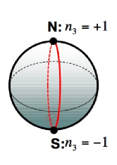
Figure 8: The embedding of the sine-Gordon model into the ${\mathbb{C}}P^{1}$ model. The great circle $S^{1}$ denotes the target space of the sine-Gordon model. N and S are two vacua $\Theta=0$ and $\Theta=\pi$ modulo $2\pi$ of the sine-Gordon model.

To see the correspondence between instantons in the ${\mathbb{C}}P^{1}$ model and reduced sine-Gordon model, let us first examine the BPS one-instanton solution in Eq.(92), whose inhomogeneous coordinate is given as

$$\frac{H_{1}}{H_{2}}=\frac{H_{0,1}^{\mathcal{I}}}{H_{0,2}^{\mathcal{I}}}=\lambda e^{i\phi}e^{-\frac{\pi z}{L}}=\lambda e^{-\frac{\pi x_{1}}{L}+i(\phi-\frac{\pi x_{2}}{L})},$$ (102)

$$\Phi(x_{1},x_{2})=\phi-\frac{\pi x_{2}}{L},\quad\Theta(x_{1},x_{2})=2\arctan\left(e^{\frac{\pi}{L}(x_{1}-\frac{L}{\pi}\log\lambda)}\right).$$ (103)

We see that this solution is consistent with the assumption of the Scherk-Schwarz reduction in Eq.(96) with Eq.(99). This solution gives the vertical path starting from N at $x_{1}=-\infty$ and reaching S at $x_{1}=\infty$ with $\Phi=0$ when $x_{2}=0$. With varying from $x_{2}=0$ to $x_{2}=L$, this vertical path revolves in $\Phi$ to end up at $x_{2}=L$ with another vertical path connecting N (at $x_{1}=-\infty$) to S (at $x_{1}=\infty$) with $\Phi=\pi$. Thus the paths sweep precisely half of $S^{2}$, as illustrated in Fig. 9. The solution $\Theta$ in Eq. (103) is identical to the single instanton solution of the sine-Gordon quantum mechanics in Eq.(13). Therefore the fractional instanton solution of the ${\mathbb{C}}P^{1}$ model is captured correctly by the sine-Gordon quantum mechanics as the instanton solution. The second homotopy group $\pi_{2}$ for the ${\mathbb{C}}P^{1}$ fractional instanton is 1/2, while the first homotopy group $\pi_{1}$ for the reduced sine-Gordon model is also 1/2 because it corresponds to a half orbit of the great circle.

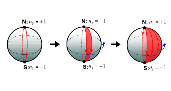
Figure 9: Fractional instanton configuration on $S^{2}$ in the reduced quantum mechanics is depicted. It corresponds to a single line from the north to the south pole which is rotated over the half of $S^{2}$ homogeneously. The figure depicts the rotation of the line around the half sphere. The red arrows denote paths depending on $x_{2}$ with a constant $x_{1}$, while the blue arrows denote the $x_{1}$ dependence of such paths.

In Fig. 10, we classify how all possible (anti-)instanton configurations in the reduced sine-Gordon model correspond to the fractional instantons in the original ${\mathbb{C}}P^{1}$ model. As shown in Eqs. (16) and (17), a sine-Gordon soliton connecting from a vacuum labeled by even $n$ to a vacuum labeled by odd $n$ is BPS while that from odd $n$ to even $n$ is anti-BPS. When the sine-Gordon quantum mechanics is embedded into the ${\mathbb{C}}P^{1}$ model, a soliton from N to S on $S^{2}$ is BPS while that from S to N is anti-BPS, consistent with BPS and anti-BPS kinks in the ${\mathbb{C}}P^{1}$ model. In other words, configurations with positive values of the second homotopy class $\pi_{2}$ are BPS while those with negative values are anti-BPS both in the ${\mathbb{C}}P^{1}$ model and reduced sine-Gordon model. Thus, (a) and (d) in Fig. 10 are BPS while (b) and (c) are anti-BPS.

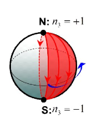
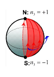
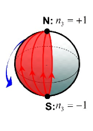
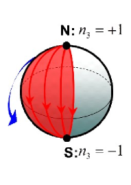
$\pi_{1}$	$+1/2$	$-1/2$	$+1/2$	$-1/2$
$\pi_{2}$	$+1/2$	$-1/2$	$-1/2$	$+1/2$
	(a)	(b)	(c)	(d)

Figure 10: Fractional (anti-)instanton configurations in the reduced quantum mechanics is depicted on the $S^{2}$ target space of the ${\mathbb{C}}P^{1}$ model. The first and second homotopy groups for instantons in the sine-Gordon model and ${\mathbb{C}}P^{1}$ model are shown. Configurations with positive values of the second homotopy class $\pi_{2}$ are BPS while those with negative values are anti-BPS both in the ${\mathbb{C}}P^{1}$ model and reduced sine-Gordon model. Thus, (a) and (d) are BPS while (b) and (c) are anti-BPS.

Here we point out that the BPS solution of two fractional-instantons in the ${\mathbb{C}}P^{1}$ model cannot be described in the reduced sine-Gordon model. The BPS solution of two fractional-instantons, which contains the ordinary one-instanton BPS solution ($Q=1$) in the limit of small separation of two fractional instantons is given by

$$H_{0}^{\cal II}(z)=\left(\lambda_{1}e^{i\phi_{1}}e^{-\frac{\pi z}{L}}+\lambda_{2}e^{i\phi_{2}}e^{\frac{\pi z}{L}},1\right).$$ (104)

This is a composite of (a) and (d) in Fig.10. The inhomogeneous coordinate of ${\mathbb{C}}P^{1}$ now reads

$$\frac{H_{1}^{\cal II}}{H_{2}^{\cal II}}=\frac{H_{0,1}^{\cal II}}{H_{0,2}^{\cal II}}=\lambda_{1}e^{-\frac{\pi x_{1}}{L}}e^{i(\phi_{1}-\frac{\pi x_{2}}{L})}+\lambda_{2}e^{\frac{\pi x_{1}}{L}}e^{i(\phi_{2}+\frac{\pi x_{2}}{L})},$$ (105)

which cannot satisfy the assumption (96) of the Scherk-Schwarz reduction. This is because in the reduced sine-Gordon model a configuration starting from N and ending at S [(a) in Fig. 10] cannot be connected to another configuration starting from N and ending at S [(d) in Fig. 10]. The former can be connected only to a configuration starting from S and ending at N. Therefore the BPS two fractional instanton solution cannot be described by the sine-Gordon quantum mechanics even in the limit of small $L$. More generally, all the BPS multi-fractional-instanton solutions are inconsistent with the Scherk-Schwarz reduction and hence the sine-Gordon quantum mechanics fails to capture them. This is consistent with the fact that configurations containing $n$-instantons ($n\geq 2$) are always non-BPS in the sine-Gordon quantum mechanics.

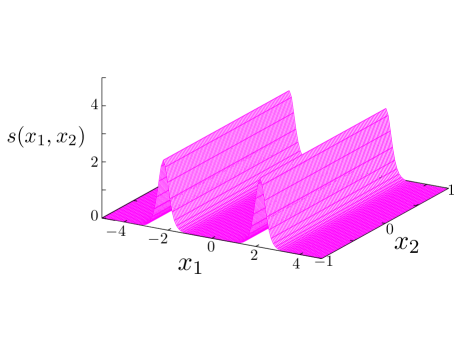
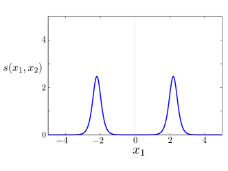
Figure 11: The euclidean action density $s(x_{1},x_{2})$ of neutral bion configurations for $\lambda_{1}=1/1000,\lambda_{2}=1/1000$ and $\phi=\pi/4$ in the ${\mathbb{C}}P^{1}$ model on ${\mathbb{R}}^{1}\times S^{1}$. The same action density is depicted in two ways, as a function of $x_{1},x_{2}$ (left) and $x_{1}$ (right). There is no $x_{2}$ dependence in the action density, with $x_{2}$ being a coordinate of the compactied dimension.

Next let us consider the non-BPS configuration of neutral bion, which is a composite of a fractional instanton and a fractional anti-instanton as depicted in Fig. 11. We can write down an Ansatz for the moduli matrix $H_{0}$

$$H_{0}^{\cal I\bar{I}}(z,\bar{z})=\left(\lambda_{1}e^{i\phi_{1}}e^{-\frac{\pi z}{L}}+\lambda_{2}e^{i\phi_{2}}e^{\frac{\pi\bar{z}}{L}},1\right),$$ (106)

which is guaranteed to become an exact solution of the field equation in the limit of large separation ($-\frac{L}{\pi}\log(\lambda_{1}\lambda_{2})\to\infty$) between constituents. The inhomogeneous coordinate of ${\mathbb{C}}P^{1}$ now reads

$$\frac{H_{1}^{\cal I\bar{I}}}{H_{2}^{\cal I\bar{I}}}=\frac{H_{0,1}^{\cal I\bar{I}}}{H_{0,2}^{\cal I\bar{I}}}=\left(\lambda_{1}e^{-\frac{\pi x_{1}}{L}}+\lambda_{2}e^{\frac{\pi x_{1}}{L}}e^{i(\phi_{2}-\phi_{1})}\right)e^{i(\phi_{1}-\frac{\pi x_{2}}{L})},$$ (107)

which satisfy the assumption (96) of the Scherk-Schwarz reduction if and only if $e^{i(\phi_{2}-\phi_{1})}=\mp 1$. In that case, we obtain the angular coordinate fields of $S^{2}$ as

$$\Phi(x_{1},x_{2})=\phi_{1}-\frac{\pi x_{2}}{L},\quad\cot\frac{\Theta(x_{1},x_{2})}{2}=\lambda_{1}e^{-\frac{\pi x_{1}}{L}}\mp\lambda_{2}e^{\frac{\pi x_{1}}{L}}.$$ (108)

This configuration starts from N at $x_{1}=-\infty$. For the upper sign, it goes through S at $x_{1}=-\frac{L}{\pi}\log(\lambda_{1}\lambda_{2})$ and reaches to N with $\Theta=2\pi$ at $x_{1}=\infty$, namely it winds once around the great circle. The configuration represents the double instanton configuration of the sine-Gordon quantum mechanics as shown in Fig.1. For the lower sign, the configuration returns back to N with $\Theta=0$ at $x_{1}=\infty$ approaching but never reaching S at any point in $-\infty<x_{1}<\infty$. This clearly represents the instanton and anti-instanton configuration $[\mathcal{I}\bar{\mathcal{I}}]$ of the sine-Gordon quantum mechanics, as shown in the left panel of Fig. 2. The sine-Gordon quantum mechanics captures only field configurations that can cover the (part of) $S^{2}$ in the following specific fashion : When $x_{1}$ is varied with fixed $x_{2}$, $\Theta$ goes along the great circle (namely fixed $\Phi$), whereas $x_{2}$ variation with fixed $x_{1}$ makes a rotation of $\Phi$ with the constant velocity by an amount $\pi$ at fixed $\Theta$. The first homotopy group $\pi_{1}$ for the sine-Gordon model is one for the upper sign and zero for the lower sign, but the second homotopy group $\pi_{2}$ for the ${\mathbb{C}}P^{1}$ model is zero for the both cases. In Fig. 12, we show the instanton–anti-instanton and instanton-instanton configurations in the sine-Gordon quantum mechanics corresponding to $e^{i(\phi_{2}-\phi_{1})}=\mp 1$ in Eq. (107), and how the corresponding configuration of the ${\mathbb{C}}P^{1}$ model in Eq.(108) cover the sphere $S^{2}$. Here, each of fractional instanton again corresponds to the line between the north and south poles sweeping around the half sphere.

On the other hand, generic configurations of the neutral bion of the ${\mathbb{C}}P^{1}$ model in Eq. (107) exhibit complicated ways of covering (part of) $S^{2}$ in terms of $\Theta,\Phi$. In terms of the $H(x_{1},x_{2})$ field, however, they are quite similar to those special configurations with $e^{i(\phi_{2}-\phi_{1})}=\mp 1$ describable by the sine-Gordon quantum mechanics except for an important new feature : they have the relative phase $e^{i(\phi_{2}-\phi_{1})}$ between fractional instanton and anti-instanton as an additional moduli of the neutral bion configuration. This relative phase moduli introduces a striking physical effect into interactions between fractional instanton and anti-instanton constituents even in the limit of $L\to 0$, as we see immediately.

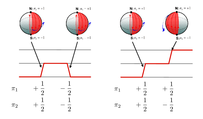
Figure 12: One fractional instanton and anti-instanton(left) and two fractional instantons (right) in the ${\mathbb{C}}P^{1}$ model are depicted.

The absence of the relative phase moduli between the instanton constituents in the bion configuration is a crucial drawback of the sine-Gordon quantam mechanical description. To clarify how crucial it is, we discuss the neutral bion configuration in the ${\mathbb{C}}P^{N-1}$ model on ${\mathbb{R}}^{1}\times S^{1}$ with the ${\mathbb{Z}}_{N}$ twisted boundary conditions. Generalizing Eq.(106) in the ${\mathbb{C}}P^{1}$ model, the neutral bion configuration with the relative phase moduli between the two constituents is given by Misumi:2014jua

$$H_{0}^{\mathcal{I}\bar{\mathcal{I}}}\,=\,\left(\lambda_{1}\,e^{-{2\pi\over{NL}}z}+e^{i\phi}\lambda_{2}e^{{2\pi\over{NL}}\bar{z}},1,0...,0\right)\,,$$ (109)

where $\lambda_{1},\lambda_{2}$ are real parameters corresponding to positions of constituent fractional instanton and fractional anti-instanton, and $\phi$ is the relative phase. Here, the separation between the fractional instanton and anti-instanton is given by $R=-(NL/2\pi)\log\lambda_{1}\lambda_{2}$. We study the interaction potential as a function of separation $R$ of constituents for the fixed relative phase $\phi$. As we vary this relative phase $\phi$ from $0$ to $2\pi$, we find that the interaction between the instanton and anti-instanton constituents is attractive for $0\leq\phi<\pi/2$ and $3\pi/2<\phi\leq 2\pi$, whereas it is repulsive for $\pi/2<\phi<3\pi/2$. We compare the energy density for various relative phases in Fig. 13. The interaction potential between fractional instanton and fractional anti-instanton is derived by both numerically Misumi:2014jua and analytically as

$$V[R]\,=\,-{4\kappa Lv^{2}\cos\phi}\,\exp(-\kappa R)\,,$$ (110)

where we note $\kappa\equiv 2\pi/(NL)$ and the coupling of ${\mathbb{C}}P^{N-1}$ model is denoted as $1/v$. We here follow the definition in our previous work Misumi:2014jua : Our coupling $1/v$ is related to the coupling $g_{\rm DU}$ adopted in Dunne:2012ae as $v^{2}=2/g_{\rm DU}^{2}$. We note that the corresponding configuration in the sine-Gordon quantum mechanics has no relative phase moduli and the interaction potential between the instanton and anti-instanton constituents is given by Eq. (26) with the minus sign (attraction). Therefore the neutral bion contribution in the ${\mathbb{C}}P^{N-1}$ model cannot be calculated in the reduced quantum mechanics correctly.

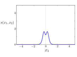
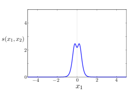
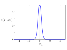
Figure 13: The euclidean action density $s(x_{1},x_{2})$ of neutral bion configurations for $\lambda_{1}=1/2,\lambda_{2}=1/2$ are shown for several values of relative phase moduli $\phi$ : $\phi=0$ (left), $\pi/2$ (center) and $\pi$ (right). The total action increases as the relative phase $\phi$ is varied from $0$ to $\pi$, while configurations in a far-separated situation are almost the same for the three cases. The attractive force decreases in the region from $\phi=0$ to $\phi=\pi/2$, then becomes repulsive for $\pi/2<\phi<\pi$.

The neutral bion amplitude has been computed previously by ignoring the relative phase moduli ($\phi=0$). The result can be given in terms of the dimensionless separation variable $\tau=\kappa R$ Dunne:2012ae ; Misumi:2014bsa

$$[{\mathcal{B}}_{ii}]^{\phi=0} = Ce^{-2S_{I}/N}I(v^{2}),$$

$$I(v^{2}) = \int_{0}^{\infty}d\tau\exp\left(4\kappa Lv^{2}e^{-\tau}-\epsilon\tau\right)=\int_{0}^{\infty}d\tau\exp\left(\frac{8\pi v^{2}}{N}e^{-\tau}-\epsilon\tau\right)$$ (111)

$$= -\left(\gamma+\log\left(\frac{8\pi v^{2}}{N}\right)\right)\mp i\pi,$$

where $S_{I}=2\pi v^{2}$ is the instanton action and $C$ denotes the numerical coefficient when the relative phase moduli is ignored ($\phi=0$). Based on the interaction potential we obtained in Eq. (110), we find that the corrected contributions of the neutral bion is given by taking account of the relative phase moduli as

$$[{\mathcal{B}}_{ii}]=Ce^{-2S_{I}/N}\int_{0}^{2\pi}d\phi\,I(v^{2}\cos\phi).$$ (112)

Since the moduli integrals for $[0,\pi]$ and $[\pi,2\pi]$ are identical, we will double the result for $[0,\pi]$. We apply the BZJ prescription to the integral in the case of the attractive interaction for $[0,\pi/2]$, while we simply perform the integral for the repulsive case $[\pi/2,\pi]$. Using Eqs.(29) and (32), we obtain

$$\int_{0}^{2\pi}d \phi\,I(v^{2}\cos\phi)$$

$$=2\left[\int_{0}^{\pi/2}d\phi\left\{-\left(\gamma+\log\left(\frac{8\pi v^{2}}{N}\cos\phi\right)\right)\mp i\pi\right\}+\int_{\pi/2}^{\pi}d\phi\left\{-\left(\gamma+\log\left(-\frac{8\pi v^{2}}{N}\cos\phi\right)\right)\right\}\right]$$

$$=-2\pi\left(\gamma+\log\left(\frac{4\pi v^{2}}{N}\right)\right)\,\mp\,i\pi^{2}.$$ (113)

Thus we obtain the neutral bion contribution as

$$\left[{\mathcal{B}}_{ii}\right]\,=\,Ce^{-\frac{2S_{I}}{N}}\left[-2\pi\left(\gamma+\log\left(\frac{4\pi v^{2}}{N}\right)\right)\,\mp\,i\pi^{2}\right]\,,$$ (114)

in contrast to the result in Eq.(111) where the relative phase is ignored. We have obtained quantitative corrections to that in Ref. Dunne:2012ae , by taking account of the effects of the integral of the relative phase moduli. To establish the absolute magnitude of the instanton contribution definitely, it is desirable to examine the one-loop determinant around the fractional instanton and anti-instanton background for the two-dimensional ${\mathbb{C}}P^{N-1}$ model which has an explicit (weak) dependence on $x_{2}$. We consider these as future works.

Before closing this section, we note an alternative possibility to relate the sine-Gordon quantum mechanics and the ${\mathbb{C}}P^{N-1}$ model without compactification. Even if the compactification length is nonzero, the ${\mathbb{C}}P^{1}$ model can be deformed so as to produce the sine-Gordon instanton solutions. To clarify this point, we move to the $O(3)$ non-linear sigma model equivalent to the ${\mathbb{C}}P^{1}$ model. In this model, we have three real scalar fields $n_{1},n_{2},n_{3}$ subjected by the constraint $(n_{1})^{2}+(n_{2})^{2}+(n_{3})^{2}=1$. We introduce the two potential terms $V_{1}=m^{2}(1-n_{3}^{2})$ and $V_{2}=-\triangle m^{2}n_{1}$, with a mass hierarchy $\triangle m^{2}\ll m^{2}$. For the parameter region $\triangle m^{2}\sim 0$, the potential $V_{1}$ admits two discrete vacua $n_{3}=\pm 1$ and a ${\mathbb{C}}P^{1}$ domain wall solution interpolating these two vacua Abraham:1992vb with the width $m^{-1}$. Let us place it perpendicularly to the $x_{2}$ direction. With a small $\triangle m^{2}(\neq 0)\ll m^{2}$, the above vacua are shifted and the domain wall is deformed accordingly. In this case, the sine-Gordon model is induced on the ${\mathbb{C}}P^{1}$ domain wall as the effective theory Nitta:2012xq . Then, an $O(3)$ ($\mathbb{C}P^{1}$) instanton is restricted to the ${\mathbb{C}}P^{1}$ domain wall and becomes a sine-Gordon instanton with the width $\triangle m^{-1}$ (in the $x_{1}$ direction), in the domain wall effective theory Nitta:2012xq . This setting gives a precise relation between the ${\mathbb{C}}P^{1}$ model and the sine-Gordon quantum mechanics. By sending $m,\triangle m$ to zero, we may be able to investigate how the contribution of the relative complex phase disappears in the reduction process from the ${\mathbb{C}}P^{1}$ model to the sine-Gordon quantum mechanics. In the case of the ${\mathbb{C}}P^{N-1}$ model, multiple $N-1$ parallel domain walls in it Gauntlett:2000ib play the role to connect the ${\mathbb{C}}P^{N-1}$ model instantons and instantons in a sine-Gordon-like model.

VI Summary and Discussion

In this paper we have calculated multi-instanton contributions in the quantum mechanics with the sine-Gordon potential by integrating out separation moduli parameters between instantons and anti-instantons in the semi-classical limit ($|g^{2}|\ll 1$). We have adopted an extended Bogomolnyi–Zinn-Justin prescription for multi-instanton configurations and the step-by-step subtraction scheme for divergent parts. We show that the imaginary parts of the multi-instanton amplitudes cancel those arising from the Borel resummation of the large-order perturbation series. We verify that our results completely agree with those based on the uniform-WKB calculations Dunne:2013ada ; Dunne:2014bca up to a four-instanton order. We have also shown that the neutral bion amplitude in ${\mathbb{C}}P^{N-1}$ model based on the potential including the relative phase moduli parameter gives corrections to the results obtained in the sine-Gordon quantum mechanics Dunne:2012ae .

Our main results, that the multi-instanton amplitudes in the sine-Gordon quantum mechanics are consistent with the large-order behavior of the perturbative calculations, and are completely reproduced by the uniform-WKB boundary conditions, strongly indicate the following facts: the uniform-WKB boundary condition provides the correct link between the perturbation series around the perturbative vacuum and non-perturbative instanton effects, and furthermore the perturbative calculation knows non-perturbative aspects of the quantum system in the first place. We can take the result as an evidence at least in the quantum mechanics, in favor of the resurgence conjecture, which gives an unambiguous and self-consistent definition of the quantum theory ZinnJustin:1982td ; ZinnJustin:1983nr ; ZinnJustin:2004ib ; ZinnJustin:2004cg ; Jentschura:2010zza ; Dunne:2013ada ; Dunne:2014bca .

As for the neutral bion in the ${\mathbb{C}}P^{N-1}$ model on ${\mathbb{R}}^{1}\times S^{1}$, we have calculated, for the first time, the neutral bion amplitude beyond the sine-Gordon quantum mechanics, with the moduli integral of the relative phase parameter, which does not exist in the sine-Gordon quantum mechanics Dunne:2012ae . As a future study, we will perform perturbative calculations and multi-instanton calculations in the ${\mathbb{C}}P^{N-1}$ model with keeping the compactified-direction dependence, then we may be able to show that its large-order behavior of the perturbations originates in the imaginary part of the neutral-bion and bion-molecule amplitude at the field theory level.

We here make a comment on the relation of the configuration Eq. (109) to the Lefschetz thimble LT . In the recent attempt to perform the path integral in the extended theory LT , one complexifies the coupling constant (${\rm arg}[g^{2}]\not=0$) and the field variables, then the standard path integral can be replaced by the integral along the steepest descent curves in the complex configuration space, or Lefschetz thimbles with the imaginary part of the action being constant ${\rm Im}[S]={\rm const.}$. In terms of this method, the configuration Eq. (109) corresponds to the special thimble for ${\rm arg}[g^{2}]=0$, called the Stokes line, where the two critical points, in which fractional instantons are infinitely-separated or completely compressed, are directly connected by the configuration. Although, for a general case ${\rm arg}[g^{2}]\not=0$, the two critical points should belong to two different Lefschetz thimbles, our study on the Stokes line ${\rm arg}[g^{2}]=0$ could be a good starting point for investigating the general Lefschetz thimbles. Part of future work will be devoted to this study. We also note that the relation of Lefschetz thimbles and the topologically neutral configurations has been investigated in terms of the hidden topological angles in Ref. Behtash:2015kna .

We also comment that the cancellation of imaginary ambiguities in the sine-Gordon quantum mechanics, or the resurgent structure in the system, can be understood as a special case of the generic resummation structure, called “median resummation” Aniceto:2013fka . It is expected that this resummation is applicable to any quantum theories including quantum mechanics and field theory. Thus, we consider that it is intriguing to study the application of the median resummation to the sine-Gordon quantum mechanics and verify its structure as a future work.

Appendix A Calculation of $G_{i}$ ($i=1,...,6$)

In this appendix we show the details of calculation of the functions $G_{i}(g^{2})$ ($i=1,2,3,4,5,6$). The functions $G_{1},G_{2},G_{3}$ are based on the three subtraction patterns of the integral in Eq. (50). They are given by

$$G_{1}(g^{2}) \,\overset{|g^{2}|,|\tilde{g}^{2}|\ll 1}{\longrightarrow}\,\left({g^{2}\over{2}}\right)^{\epsilon}\Gamma(\epsilon)\left[\left({g^{2}\over{2}}\right)^{\epsilon}\Gamma(\epsilon)\left[\left({-\tilde{g}^{2}\over{2}}\right)^{\epsilon}\Gamma(\epsilon)-{1\over{\epsilon}}\right]+{\gamma+\log(2/(-\tilde{g}^{2}))\over{\epsilon}}\right]$$

$$\,\overset{-\tilde{g}^{2}=\tilde{g}^{2}e^{\mp i\pi}}{\longrightarrow}\,-{8\over{3}}\left(\gamma+\log{2\over{g^{2}}}\right)^{3}\,+\,{7\over{6}}\pi^{2}\left(\gamma+\log{2\over{g^{2}}}\right)+{1\over{6}}\psi^{(2)}(1)$$

$$\qquad\qquad\qquad\,\mp\,4i\pi\left(\gamma+\log{2\over{g^{2}}}\right)^{2}\,+\,O\left(\frac{1}{\epsilon}\right)\,+\,O(\epsilon)\,,$$ (115)

$$G_{2}(g^{2}) \,\overset{|g^{2}|,|\tilde{g}^{2}|\ll 1}{\longrightarrow}\,\left({g^{2}\over{2}}\right)^{\epsilon}\Gamma(\epsilon)\left[\left({-\tilde{g}^{2}\over{2}}\right)^{\epsilon}\Gamma(\epsilon)\left[\left({g^{2}\over{2}}\right)^{\epsilon}\Gamma(\epsilon)-{1\over{\epsilon}}\right]+{\gamma+\log(2/g^{2})\over{\epsilon}}\right]$$

$$\,\overset{-\tilde{g}^{2}=\tilde{g}^{2}e^{\mp i\pi}}{\longrightarrow}\,-{8\over{3}}\left(\gamma+\log{2\over{g^{2}}}\right)^{3}\,+\,{1\over{6}}\pi^{2}\left(\gamma+\log{2\over{g^{2}}}\right)+{1\over{6}}\psi^{(2)}(1)$$

$$\qquad\qquad\qquad\,\mp\,i\pi\Big{[}{5\over{2}}\left(\gamma+\log{2\over{g^{2}}}\right)^{2}+{\pi^{2}\over{12}}\Big{]}\,+\,O\left(\frac{1}{\epsilon}\right)\,+\,O(\epsilon)\,,$$ (116)

$$G_{3}(g^{2}) \,\overset{|g^{2}|,|\tilde{g}^{2}|\ll 1}{\longrightarrow}\,\left({-\tilde{g}^{2}\over{2}}\right)^{\epsilon}\Gamma(\epsilon)\left[\left({g^{2}\over{2}}\right)^{\epsilon}\Gamma(\epsilon)\left[\left({g^{2}\over{2}}\right)^{\epsilon}\Gamma(\epsilon)-{1\over{\epsilon}}\right]+{\gamma+\log(2/g^{2})\over{\epsilon}}\right]$$

$$\,\overset{-\tilde{g}^{2}=\tilde{g}^{2}e^{\mp i\pi}}{\longrightarrow}\,-{8\over{3}}\left(\gamma+\log{2\over{g^{2}}}\right)^{3}\,-\,{1\over{3}}\pi^{2}\left(\gamma+\log{2\over{g^{2}}}\right)+{1\over{6}}\psi^{(2)}(1)$$

$$\qquad\qquad\qquad\mp\,i\pi\Big{[}{3\over{2}}\left(\gamma+\log{2\over{g^{2}}}\right)^{2}+{\pi^{2}\over{12}}\Big{]}\,+\,O\left(\frac{1}{\epsilon}\right)\,+\,O(\epsilon)\,.$$ (117)

The functions $G_{4},G_{5},G_{6}$ are based on the three patterns of subtraction in the integral Eq. (53). They are given by

$$G_{4}(g^{2}) \,\overset{|g^{2}|,|\tilde{g}^{2}|\ll 1}{\longrightarrow}\,\left({-\tilde{g}^{2}\over{2}}\right)^{\epsilon}\Gamma(\epsilon)\left[\left({-\tilde{g}^{2}\over{2}}\right)^{\epsilon}\Gamma(\epsilon)\left[\left({g^{2}\over{2}}\right)^{\epsilon}\Gamma(\epsilon)-{1\over{\epsilon}}\right]+{\gamma+\log(2/g^{2})\over{\epsilon}}\right]$$

$$\,\overset{-\tilde{g}^{2}=\tilde{g}^{2}e^{\mp i\pi}}{\longrightarrow}\,-{8\over{3}}\left(\gamma+\log{2\over{g^{2}}}\right)^{3}\,+\,{7\over{6}}\pi^{2}\left(\gamma+\log{2\over{g^{2}}}\right)+{1\over{6}}\psi^{(2)}(1)$$

$$\qquad\qquad\qquad\,\mp\,i\pi\Big{[}4\left(\gamma+\log{2\over{g^{2}}}\right)^{2}+{\pi^{2}\over{6}}\Big{]}\,+\,O\left(\frac{1}{\epsilon}\right)\,+\,O(\epsilon)\,,$$ (118)

$$G_{5}(g^{2}) \,\overset{|g^{2}|,|\tilde{g}^{2}|\ll 1}{\longrightarrow}\,\left({-\tilde{g}^{2}\over{2}}\right)^{\epsilon}\Gamma(\epsilon)\left[\left({g^{2}\over{2}}\right)^{\epsilon}\Gamma(\epsilon)\left[\left({-\tilde{g}^{2}\over{2}}\right)^{\epsilon}\Gamma(\epsilon)-{1\over{\epsilon}}\right]+{\gamma+\log(2/(-\tilde{g}^{2}))\over{\epsilon}}\right]$$

$$\,\overset{-\tilde{g}^{2}=\tilde{g}^{2}e^{\mp i\pi}}{\longrightarrow}\,-{8\over{3}}\left(\gamma+\log{2\over{g^{2}}}\right)^{3}\,+\,{19\over{6}}\pi^{2}\left(\gamma+\log{2\over{g^{2}}}\right)+{1\over{6}}\psi^{(2)}(1)$$

$$\qquad\qquad\qquad\,\mp\,i\pi\Big{[}{11\over{2}}\left(\gamma+\log{2\over{g^{2}}}\right)^{2}-{5\pi^{2}\over{12}}\Big{]}\,+\,O\left(\frac{1}{\epsilon}\right)\,+\,O(\epsilon)\,,$$ (119)

$$G_{6}(g^{2}) \,\overset{|g^{2}|,|\tilde{g}^{2}|\ll 1}{\longrightarrow}\,\left({g^{2}\over{2}}\right)^{\epsilon}\Gamma(\epsilon)\left[\left({-\tilde{g}^{2}\over{2}}\right)^{\epsilon}\Gamma(\epsilon)\left[\left({-\tilde{g}^{2}\over{2}}\right)^{\epsilon}\Gamma(\epsilon)-{1\over{\epsilon}}\right]+{\gamma+\log(2/(-\tilde{g}^{2}))\over{\epsilon}}\right]$$

$$\,\overset{-\tilde{g}^{2}=\tilde{g}^{2}e^{\mp i\pi}}{\longrightarrow}\,-{8\over{3}}\left(\gamma+\log{2\over{g^{2}}}\right)^{3}\,+\,{14\over{3}}\pi^{2}\left(\gamma+\log{2\over{g^{2}}}\right)+{1\over{6}}\psi^{(2)}(1)$$

$$\qquad\qquad\qquad\,\mp\,i\pi\Big{[}{13\over{2}}\left(\gamma+\log{2\over{g^{2}}}\right)^{2}-{11\pi^{2}\over{12}}\Big{]}\,+\,O\left(\frac{1}{\epsilon}\right)\,+\,O(\epsilon)\,.$$ (120)

In the final expressions, we implicitly return $\tilde{g}^{2}$ to $g^{2}$.

References

- (1) M. Ünsal, “Abelian duality, confinement, and chiral symmetry breaking in QCD(adj),” Phys. Rev. Lett. 100, 032005 (2008) [arXiv:0708.1772 [hep-th]].
- (2) M. Ünsal, “Magnetic bion condensation: A New mechanism of confinement and mass gap in four dimensions,” Phys. Rev. D 80, 065001 (2009) [arXiv:0709.3269 [hep-th]].
- (3) M. Shifman and M. Ünsal, “QCD-like Theories on R(3) x S(1): A Smooth Journey from Small to Large r(S(1)) with Double-Trace Deformations,” Phys. Rev. D 78, 065004 (2008) [arXiv:0802.1232 [hep-th]].
- (4) E. Poppitz and M. Ünsal, “Conformality or confinement: (IR)relevance of topological excitations,” JHEP 0909, 050 (2009) [arXiv:0906.5156 [hep-th]].
- (5) M. M. Anber and E. Poppitz, “Microscopic Structure of Magnetic Bions,” JHEP 1106, 136 (2011) [arXiv:1105.0940 [hep-th]].
- (6) E. Poppitz, T. Schaefer and M. Ünsal, “Continuity, Deconfinement, and (Super) Yang-Mills Theory,” JHEP 1210, 115 (2012) [arXiv:1205.0290 [hep-th]].
- (7) P. Argyres and M. Ünsal, “A semiclassical realization of infrared renormalons,” Phys. Rev. Lett. 109, 121601 (2012) [arXiv:1204.1661 [hep-th]].
- (8) P. C. Argyres and M. Ünsal, “The semi-classical expansion and resurgence in gauge theories: new perturbative, instanton, bion, and renormalon effects,” JHEP 1208, 063 (2012) [arXiv:1206.1890 [hep-th]].
- (9) G. V. Dunne and M. Ünsal, “Resurgence and Trans-series in Quantum Field Theory: The CP(N-1) Model,” JHEP 1211, 170 (2012) [arXiv:1210.2423 [hep-th]].
- (10) G. V. Dunne and M. Ünsal, “Continuity and Resurgence: towards a continuum definition of the CP(N-1) model,” Phys. Rev. D 87, 025015 (2013) [arXiv:1210.3646 [hep-th]].
- (11) R. Dabrowski and G. V. Dunne, “Fractionalized Non-Self-Dual Solutions in the CP(N-1) Model,” Phys. Rev. D 88, 025020 (2013) [arXiv:1306.0921 [hep-th]].
- (12) G. V. Dunne and M. Ünsal, “Generating Non-perturbative Physics from Perturbation Theory,” Phys. Rev. D 89, 041701 (2014) [arXiv:1306.4405 [hep-th]].
- (13) A. Cherman, D. Dorigoni, G. V. Dunne and M. Ünsal, “Resurgence in QFT: Unitons, Fractons and Renormalons in the Principal Chiral Model,” Phys. Rev. Lett. 112, 021601 (2014) [arXiv:1308.0127 [hep-th]].
- (14) G. Basar, G. V. Dunne and M. Ünsal, “Resurgence theory, ghost-instantons, and analytic continuation of path integrals,” JHEP 1310, 041 (2013) [arXiv:1308.1108 [hep-th]].
- (15) G. V. Dunne and M. Ünsal, “Uniform WKB, Multi-instantons, and Resurgent Trans-Series,” Phys. Rev. D 89, 105009 (2014) [arXiv:1401.5202 [hep-th]].
- (16) A. Cherman, D. Dorigoni and M. Ünsal, “Decoding perturbation theory using resurgence: Stokes phenomena, new saddle points and Lefschetz thimbles,” arXiv:1403.1277 [hep-th].
- (17) A. Behtash, T. Sulejmanpasic, T. Schaefer and M. Unsal, “Hidden topological angles and Lefschetz thimbles,” arXiv:1502.06624 [hep-th].
- (18) S. Bolognesi and W. Zakrzewski, “Clustering and decomposition for non BPS solutions of the models,” Phys. Rev. D 89, 065013 (2014) [arXiv:1310.8247 [hep-th]].
- (19) T. Misumi, M. Nitta and N. Sakai, “Neutral bions in the model,” JHEP 1406, 164 (2014) [arXiv:1404.7225 [hep-th]]; T. Misumi, M. Nitta and N. Sakai, “Neutral bions in the model for resurgence,” J. Phys. Conf. Ser. 597, no. 1, 012060 (2015) [arXiv:1412.0861 [hep-th]].
- (20) S. Shermer, “Twisted CP(N-1) instanton projectors and the N-level quantum density matrix,” arXiv:1412.3185 [hep-th].
- (21) T. Misumi and T. Kanazawa, “Adjoint QCD on with twisted fermionic boundary conditions,” JHEP 1406, 181 (2014) [arXiv:1405.3113 [hep-ph]].
- (22) T. Misumi, M. Nitta and N. Sakai, “Classifying bions in Grassmann sigma models and non-Abelian gauge theories by D-branes,” PTEP 2015, 033B02 (2015) [arXiv:1409.3444 [hep-th]].
- (23) M. Nitta, “Fractional instantons and bions in the principal chiral model on with twisted boundary conditions,” arXiv:1503.06336 [hep-th].
- (24) M. Nitta, “Fractional instantons and bions in the O model with twisted boundary conditions,” JHEP 1503, 108 (2015) [arXiv:1412.7681 [hep-th]].
- (25) G. V. Dunne and M. Unsal, “Resurgence and Dynamics of O(N) and Grassmannian Sigma Models,” arXiv:1505.07803 [hep-th].
- (26) G. ’t Hooft, “Can We Make Sense Out of Quantum Chromodynamics?,” Subnucl. Ser. 15, 943 (1979).
- (27) V. A. Fateev, V. A. Kazakov and P. B. Wiegmann, “Principal chiral field at large N,” Nucl. Phys. B 424, 505 (1994) [hep-th/9403099].
- (28) V. A. Fateev, P. B. Wiegmann and V. A. Kazakov, “Large N chiral field in two-dimensions,” Phys. Rev. Lett. 73, 1750 (1994).
- (29) J. Ecalle, “Les Fonctions Resurgentes”, Vol. I - III (Publ. Math. Orsay, 1981).
- (30) M. Marino, R. Schiappa and M. Weiss, “Nonperturbative Effects and the Large-Order Behavior of Matrix Models and Topological Strings,” Commun. Num. Theor. Phys. 2, 349 (2008) [arXiv:0711.1954 [hep-th]].
- (31) M. Marino, “Nonperturbative effects and nonperturbative definitions in matrix models and topological strings,” JHEP 0812, 114 (2008) [arXiv:0805.3033 [hep-th]].
- (32) M. Marino, R. Schiappa and M. Weiss, “Multi-Instantons and Multi-Cuts,” J. Math. Phys. 50, 052301 (2009) [arXiv:0809.2619 [hep-th]].
- (33) S. Pasquetti and R. Schiappa, “Borel and Stokes Nonperturbative Phenomena in Topological String Theory and c=1 Matrix Models,” Annales Henri Poincare 11, 351 (2010) [arXiv:0907.4082 [hep-th]].
- (34) N. Drukker, M. Marino and P. Putrov, “From weak to strong coupling in ABJM theory,” Commun. Math. Phys. 306, 511 (2011) [arXiv:1007.3837 [hep-th]].
- (35) I. Aniceto, R. Schiappa and M. Vonk, “The Resurgence of Instantons in String Theory,” Commun. Num. Theor. Phys. 6, 339 (2012) [arXiv:1106.5922 [hep-th]].
- (36) M. Marino, “Lectures on non-perturbative effects in large gauge theories, matrix models and strings,” Fortsch. Phys. 62, 455 (2014) [arXiv:1206.6272 [hep-th]].
- (37) Y. Hatsuda, S. Moriyama and K. Okuyama, “Instanton Bound States in ABJM Theory,” JHEP 1305, 054 (2013) [arXiv:1301.5184 [hep-th]].
- (38) R. Schiappa and R. Vaz, “The Resurgence of Instantons: Multi-Cut Stokes Phases and the Painleve II Equation,” Commun. Math. Phys. 330, 655 (2014) [arXiv:1302.5138 [hep-th]].
- (39) Y. Hatsuda, M. Marino, S. Moriyama and K. Okuyama, “Non-perturbative effects and the refined topological string,” JHEP 1409, 168 (2014) [arXiv:1306.1734 [hep-th]].
- (40) I. Aniceto and R. Schiappa, “Nonperturbative Ambiguities and the Reality of Resurgent Transseries,” Commun. Math. Phys. 335, no. 1, 183 (2015) [arXiv:1308.1115 [hep-th]].
- (41) R. C. Santamaria, J. D. Edelstein, R. Schiappa and M. Vonk, “Resurgent Transseries and the Holomorphic Anomaly,” arXiv:1308.1695 [hep-th].
- (42) J. Kallen and M. Marino, “Instanton effects and quantum spectral curves,” arXiv:1308.6485 [hep-th].
- (43) M. Honda and S. Moriyama, “Instanton Effects in Orbifold ABJM Theory,” JHEP 1408, 091 (2014) [arXiv:1404.0676 [hep-th]].
- (44) A. Grassi, M. Marino and S. Zakany, “Resumming the string perturbation series,” JHEP 1505, 038 (2015) [arXiv:1405.4214 [hep-th]].
- (45) D. Sauzin, “Introduction to 1-summability and resurgence, ” arXiv:1405.0356 [math.DS].
- (46) J. Kallen, “The spectral problem of the ABJ Fermi gas,” arXiv:1407.0625 [hep-th].
- (47) R. Couso-Santamaria, J. D. Edelstein, R. Schiappa and M. Vonk, “Resurgent Transseries and the Holomorphic Anomaly: Nonperturbative Closed Strings in Local ,” Commun. Math. Phys. 338, no. 1, 285 (2015) [arXiv:1407.4821 [hep-th]].
- (48) M. Honda, “On Perturbation theory improved by Strong coupling expansion,” JHEP 1412, 019 (2014) [arXiv:1408.2960 [hep-th]].
- (49) I. Aniceto, J. G. Russo and R. Schiappa, “Resurgent Analysis of Localizable Observables in Supersymmetric Gauge Theories,” JHEP 1503, 172 (2015) [arXiv:1410.5834 [hep-th]].
- (50) R. Couso-Santamaria, R. Schiappa and R. Vaz, “Finite N from Resurgent Large N,” Annals Phys. 356, 1 (2015) [arXiv:1501.01007 [hep-th]].
- (51) M. Honda and D. P. Jatkar, “Interpolating function and Stokes Phenomena,” arXiv:1504.02276 [hep-th].
- (52) Y. Hatsuda and K. Okuyama, “Resummations and Non-Perturbative Corrections,” arXiv:1505.07460 [hep-th].
- (53) I. Aniceto, “The Resurgence of the Cusp Anomalous Dimension,” arXiv:1506.03388 [hep-th].
- (54) D. Dorigoni and Y. Hatsuda, “Resurgence of the Cusp Anomalous Dimension,” arXiv:1506.03763 [hep-th].
- (55) E. B. Bogomolny, “Calculation Of Instanton - Anti-instanton Contributions In Quantum Mechanics,” Phys. Lett. B 91, 431 (1980).
- (56) J. Zinn-Justin, “Multi - Instanton Contributions in Quantum Mechanics,” Nucl. Phys. B 192, 125 (1981).
- (57) J. Zinn-Justin, “Multi - Instanton Contributions in Quantum Mechanics. 2.,” Nucl. Phys. B 218 (1983) 333.
- (58) J. Zinn-Justin, “Instantons in Quantum Mechanics: Numerical Evidence for a Conjecture,” J. Math. Phys. 25 (1984) 549.
- (59) J. Zinn-Justin and U. D. Jentschura, “Multi-instantons and exact results I: Conjectures, WKB expansions, and instanton interactions,” Annals Phys. 313, 197 (2004) [quant-ph/0501136].
- (60) J. Zinn-Justin and U. D. Jentschura, “Multi-instantons and exact results II: Specific cases, higher-order effects, and numerical calculations,” Annals Phys. 313, 269 (2004) [quant-ph/0501137].
- (61) U. D. Jentschura, A. Surzhykov and J. Zinn-Justin, “Multi-instantons and exact results. III: Unification of even and odd anharmonic oscillators,” Annals Phys. 325, 1135 (2010).
- (62) U. D. Jentschura and J. Zinn-Justin, “Multi-instantons and exact results. IV: Path integral formalism,” Annals Phys. 326, 2186 (2011).
- (63) M. A. Escobar-Ruiz, E. Shuryak and A. V. Turbiner, “Three-loop Correction to the Instanton Density. I. The Quartic Double Well Potential,” arXiv:1501.03993 [hep-th]; “Three-loop Correction to the Instanton Density. II. The Sine-Gordon potential,” arXiv:1505.05115 [hep-th].
- (64) N. S. Manton and P. Sutcliffe, “Topological solitons,” Cambridge, UK: Univ. Pr. (2004) 493 p
- (65) G. Álvarez, “Langer-Cherry derivation of the multi-instanton expansion for the symmetric double well”, J. Math. Phys. 45, 3095 (2004).
- (66) R. E. Langer, “The Asymptotic Solutions of Certain Linear Ordinary Differential Equations of the Second Order”, Trans. Am. Math. Soc. 36, 90 (1934).
- (67) T. M. Cherry, “Expansions in terms of Parabolic Cylinder Functions”, Proc. Edinburgh Math. Soc. 8, 50 (1948).
- (68) S. C. Miller and R. H. Good, “A WKB-Type Approximation to the Schrödinger Equation”, Phys. Rev. 91, 174 (1953).
- (69) A. Galindo and P. Pascual, Quantum Mechanics, Vol. II (Springer, 1991).
- (70) J. Zinn-Justin, “Quantum field theory and critical phenomena,” Int. Ser. Monogr. Phys. 77, 1 (1989).
- (71) M. Eto, Y. Isozumi, M. Nitta, K. Ohashi and N. Sakai, “Instantons in the Higgs phase,” Phys. Rev. D 72, 025011 (2005) [hep-th/0412048].
- (72) M. Eto, T. Fujimori, Y. Isozumi, M. Nitta, K. Ohashi, K. Ohta and N. Sakai, “Non-Abelian vortices on cylinder: Duality between vortices and walls,” Phys. Rev. D 73, 085008 (2006) [hep-th/0601181]; M. Eto, T. Fujimori, M. Nitta, K. Ohashi, K. Ohta and N. Sakai, “Statistical mechanics of vortices from D-branes and T-duality,” Nucl. Phys. B 788, 120 (2008) [hep-th/0703197].
- (73) M. Eto, Y. Isozumi, M. Nitta, K. Ohashi and N. Sakai, “Solitons in the Higgs phase: The Moduli matrix approach,” J. Phys. A 39, R315 (2006) [hep-th/0602170].
- (74) F. Bruckmann, “Instanton constituents in the O(3) model at finite temperature,” Phys. Rev. Lett. 100, 051602 (2008) [arXiv:0707.0775 [hep-th]]; W. Brendel, F. Bruckmann, L. Janssen, A. Wipf and C. Wozar, “Instanton constituents and fermionic zero modes in twisted CP**n models,” Phys. Lett. B 676, 116 (2009) [arXiv:0902.2328 [hep-th]]; D. Harland, “Kinks, chains, and loop groups in the CP**n sigma models,” J. Math. Phys. 50, 122902 (2009) [arXiv:0902.2303 [hep-th]]. F. Bruckmann and T. Sulejmanpasic, “Nonlinear sigma models at nonzero chemical potential: breaking up instantons and the phase diagram,” arXiv:1408.2229 [hep-th].
- (75) E. R. C. Abraham and P. K. Townsend, “Q kinks,” Phys. Lett. B 291, 85 (1992); E. R. C. Abraham and P. K. Townsend, “More on Q kinks: A (1+1)-dimensional analog of dyons,” Phys. Lett. B 295, 225 (1992); M. Arai, M. Naganuma, M. Nitta and N. Sakai, “Manifest supersymmetry for BPS walls in N=2 nonlinear sigma models,” Nucl. Phys. B 652, 35 (2003) [hep-th/0211103]; M. Arai, M. Naganuma, M. Nitta and N. Sakai, “BPS wall in N=2 SUSY nonlinear sigma model with Eguchi-Hanson manifold,” In *Arai, A. (ed.) et al.: A garden of quanta* 299-325 [hep-th/0302028].
- (76) J. P. Gauntlett, D. Tong and P. K. Townsend, “Multidomain walls in massive supersymmetric sigma models,” Phys. Rev. D 64, 025010 (2001) [hep-th/0012178]; Y. Isozumi, M. Nitta, K. Ohashi and N. Sakai, “Construction of non-Abelian walls and their complete moduli space,” Phys. Rev. Lett. 93, 161601 (2004) [hep-th/0404198]; Y. Isozumi, M. Nitta, K. Ohashi and N. Sakai, “Non-Abelian walls in supersymmetric gauge theories,” Phys. Rev. D 70, 125014 (2004) [hep-th/0405194]; M. Eto, Y. Isozumi, M. Nitta, K. Ohashi, K. Ohta and N. Sakai, “D-brane construction for non-Abelian walls,” Phys. Rev. D 71, 125006 (2005) [hep-th/0412024]; M. Eto, Y. Isozumi, M. Nitta, K. Ohashi, K. Ohta, N. Sakai and Y. Tachikawa, “Global structure of moduli space for BPS walls,” Phys. Rev. D 71, 105009 (2005) [hep-th/0503033].
- (77) M. Nitta, “Josephson vortices and the Atiyah-Manton construction,” Phys. Rev. D 86, 125004 (2012) [arXiv:1207.6958 [hep-th]]; M. Kobayashi and M. Nitta, “Sine-Gordon kinks on a domain wall ring,” Phys. Rev. D 87, no. 8, 085003 (2013) [arXiv:1302.0989 [hep-th]].
- (78) Y. Tanizaki, “Lefschetz-thimble techniques for path integral of zero-dimensional sigma models,” Phys. Rev. D 91, no. 3, 036002 (2015) [arXiv:1412.1891 [hep-th]]; T. Kanazawa and Y. Tanizaki, “Structure of Lefschetz thimbles in simple fermionic systems,” JHEP 1503, 044 (2015) [arXiv:1412.2802 [hep-th]]; Y. Tanizaki, H. Nishimura and K. Kashiwa, “Evading the sign problem in the mean-field approximation through Lefschetz-thimble path integral,” Phys. Rev. D 91, no. 10, 101701 (2015) [arXiv:1504.02979 [hep-th]].