Non-hydrogenic excitons in perovskite CH₃NH₃PbI₃

Abstract

The excitons in the orthorhombic phase of the perovskite CH₃NH₃PbI₃ are studied using the effective mass approximation. The electron-hole interaction is screened by a distance-dependent dielectric function, as described by the Haken potential or the Pollmann-Büttner potential. The energy spectrum and the eigenfunctions are calculated for both cases. The effective masses, the low and high frequency dielectric constants, and the interband absorption matrix elements, are obtained from generalized density functional theory calculations. The results show that the Pollmann-Büttner model provides better agreement with the experimental results. The discrete part of the exciton spectrum is composed of a fundamental state with a binding energy of 24 meV, and higher states that are within 2 meV from the onset the unbound exciton continuum. Light absorption is dominated by the fundamental line with an oscillator strength of 0.013, followed by the exciton continuum. The calculations have been performed without fitting any parameter from experiments and are in close agreement with recent experimental results.

Hybrid organic/inorganic perovskites based on lead or tin tri-halides are semiconductor materials that have revolutionized the research of thin film solar cells. With the first prototypes demonstrated six years agoKojima et al. (2009), record cell efficiencies have surpassed the barrier of 20%nre (2015); Jacoby (2014). Methyl-ammonium lead iodide (CH₃NH₃PbI₃) is one of the most studied members of this family, and it has been applied as photon absorber and charge transporting materialEtgar et al. (2012); Park (2013).

CH₃NH₃PbI₃ presents two phase transitions at $\sim 162$ K and $\sim 327$ K. At these transitions, the crystal symmetry changes first from orthorhombic to tetragonal and then to cubic symmetryKnop et al. (1990); Baikie et al. (2013); Stoumpos et al. (2013); Kawamura et al. (2002). The three phases differ by small changes of the lattice vectors, rotations of the characteristic PbI₆ octahedra, and the orientation of the CH₃NH${}_{3}^{+}$ cations. In the tetragonal and cubic phases, the CH₃NH${}_{3}^{+}$ cations present orientational and dynamic disorderWasylishen et al. (1985), with a deep effect on the dielectric propertiesLin et al. (2015); Frost et al. (2014). In the low temperature orthorhombic phase, the CH₃NH${}_{3}^{+}$ positions and orientations are fixedKnop et al. (1990); Baikie et al. (2013).

The electronic band structure of CH₃NH₃PbI₃ has been explained on the basis of generalized density functional theory (hybrid functionals) or Green functions GW calculations, in both cases including the spin-orbit couplingUmari et al. (2014); Brivio et al. (2014); Menéndez-Proupin et al. (2014). For the orthorhombic phase, the valence band maximum (VBM) and the conduction band minimum (CBM) are located at the $\Gamma$ point corresponding to the 48-atoms unit cell, and the fundamental gap is 1.68 eVIshihara (1994). Both the VBM and CBM are doubly degenerated, with nearly symmetric effective mass tensors.

Exciton peaks are observed in the light absorption spectra at low temperatureHirasawa et al. (1994); Tanaka et al. (2003); D’Innocenzo et al. (2014), just below the interband absorption edge, or melded with it, depending on the temperature. According to the Wannier-Mott modelWannier (1937); Knox (1963), the exciton is similar to a hydrogen atom with the proton and electron masses replaced by the hole and electron effective masses, and the Coulomb interaction is screened by a dielectric constant $\epsilon$. Therefore, the exciton binding energy and the Bohr radius are $Ry=\mu e^{4}/2\hbar^{2}\epsilon^{2}$ and $a_{ex}=\hbar^{2}\epsilon/\mu e^{2}$, where $\mu=m_{e}m_{h}/(m_{e}+m_{h})$ is the reduced electron-hole mass.

One distinct feature of CH₃NH₃PbI₃ is the large difference between the static dielectric constant $\epsilon_{0}$ and the high frequency constant $\epsilon_{\infty}$, i.e., for frequencies higher than those of the phonon absorption. Values of $\epsilon_{\infty}$ in the range $4.5-6.5$ have been calculatedBrivio et al. (2013); Umari et al. (2014); Menéndez-Proupin et al. (2014); Brivio et al. (2014), while values close to 25 have been estimated for $\epsilon_{0}$Brivio et al. (2013, 2014). Such difference is larger than in traditional inorganic semiconductor and should cause important polaron effects, such as the effective mass and gap renormalization, as well as and non-hydrogenic exciton states. For the latter, immediately arises the question wether the screening constant $\epsilon$ should be the static dielectric constant $\epsilon_{0}$ or the high frequency $\epsilon_{\infty}$. Using the values listed in Table 1, the static and the high frequency dielectric constants lead to very different values of the exciton binding energy $Ry_{0}=2.8$ meV and $Ry_{\infty}=50$ meV, respectively. Such different energies lead to different conclusions with respect to exciton dissociation due to thermal excitation, as well as to different interpretation of luminescence and transport properties.

Early estimations of the exciton binding energyHirasawa et al. (1994); Tanaka et al. (2003) $\sim 37-50$ meV were based on measurement of the exciton diamagnetic coefficient and interpretation based on the hydrogenic model with screening by $\epsilon_{\infty}=6.5$. Recent studies of the temperature dependence of photoluminescence spectraSun et al. (2014), and numerical analysis of the absorption spectraEven et al. (2014); Miyata et al. (2015) have provided updated exciton binding energies around 16-19 meV. The latter values point to a screening constant intermediate between $\epsilon_{\infty}$ and $\epsilon_{0}$. Even et alEven et al. (2014) fitted the absorption spectrum using the Wannier-Mott exciton model and obtained an effective dielectric constant $\epsilon_{eff}=11$.

In fact, the differences between $\epsilon_{0}$ and $\epsilon_{\infty}$ express the electric polarization associated to the optical phonons and the electron-phonon interaction. The stationary states are coupled states of electronic and the vibrational phonon field. The quantum calculation of these coupled states is beyond the current capabilities of ab initio methods. Model HamiltoniansHaken (1956a, 1958); Pollmann and Büttner (1977) allow one to map the coupled electron-phonon excitations into effective electronic states, and to obtain the energies of stationary states. Even when simplifying approximations are inherent in the models, they can provide a criterium on the relevant dielectric screening constants. In this Article, we apply the model Hamiltonians of HakenHaken (1956a, 1958) and that of Pollmann and BüttnerPollmann and Büttner (1977) to the exciton spectrum. This formalism is applicable to the low temperature orthorhombic phase because in the tetragonal phase the static dielectric increases strongly, associated to the reorientation of CH₃NH${}_{3}^{+}$ cations, and the exciton effects practically disappearLin et al. (2015); Frost et al. (2014); Even et al. (2014); Miyata et al. (2015).

The strength of the interaction of electrons and optical phonons is given by the coupling constant

$$\alpha_{p}=\sqrt{me^{4}/2\hbar^{2}\epsilon_{*}^{2}E_{LO}},$$ (1)

where $E_{LO}$ is the energy of the longitudinal optical phonon. This model was developed for simple crystals that display one single LO phonon branch. For this application, we have chosen $E_{LO}$ as the shift of the main peak in the CH₃NH₃PbI₃ Raman spectrumQuarti et al. (2014). The ionic screening parameter appearing in Eq. (1) is $1/\epsilon_{*}=1/\epsilon_{\infty}-1/\epsilon_{0}$.

For transport properties, relevant after exciton dissociation, polaron masses must be considered rather than the bare electronic masses computed with fixed ions. They can be estimated using the Fröhlich’s continuum theory of the large polaronDevreese and Alexandrov (2009), which predicts

$$m^{*}=m\left(1+\frac{\alpha_{p}}{6}\right).$$

The polaron bands undergo an additional shift given by $\Delta E_{p}=-\alpha_{p}E_{LO}$. With the data of Table 1, this leads to a reduction of the electronic band gap by 95 meV.

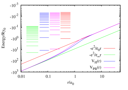
Figure 1: Haken and PB potentials compared with the Coulomb potential screened by $\epsilon_{0}$ and $\epsilon_{\infty}$. Also shown are the eigenenergies for each potential.

The Haken modelHaken (1956a, 1958) describes two interacting polarons, each one with a radius much smaller than the exciton effective radius, and expresses the effective potential for the electron-hole Coulomb interaction as

$$V_{H}(r)=-\frac{e^{2}}{\epsilon_{0}r}-\frac{e^{2}}{2\epsilon_{*}r}\left(e^{-r/l_{e}}+e^{-r/l_{h}}\right).$$ (2)

Here $l_{e,h}=\sqrt{\hbar^{2}/2m_{e,h}E_{lo}}$ are the electron- and hole-polaron radii determined using “bare” band electron and hole effective masses. The polaron effective mass parameters must be used in the kinetic energy terms of the HamiltonianHaken (1956b).

The model proposed by Pollmann and BüttnerPollmann and Büttner (1977) (PB) takes into account the correlation between electron and hole polarons, and leads to corrections to the Haken potential. The resulting electron-hole interaction potential is

$$V_{PB}(r)=-\frac{e^{2}}{\epsilon_{0}r}-\frac{e^{2}}{\epsilon_{*}r}\left(\frac{m_{h}}{\Delta m}e^{-r/l_{h}}-\frac{m_{e}}{\Delta m}e^{-r/l_{e}}\right),$$ (3)

with $\Delta m=m_{h}-m_{e}$. This potential was derived assuming $l_{e,h}$ that the polaron lengths are much smaller than the effective exciton radius, which entered as a variational parameter in the original calculationsPollmann and Büttner (1977). The bare band electron and hole masses must be used in the kinetic energy terms of the PB Hamiltonian.

Table 1: Parameters defining the polarons in CH₃NH₃PbI₃.

Dielectric constants
$\epsilon_{\infty}$	5.32
$\epsilon_{\infty}/\epsilon_{0}$	0.236
LO phonon energy
$E_{LO}$	38.5 meV
Coupling constants
$\alpha_{e}$	1.18
$\alpha_{h}$	1.28
Bare carrier masses
$m_{e}/m_{0}$	0.190
$m_{h}/m_{0}$	0.225
Polaron masses
$m_{e}^{*}/m_{0}$	0.228
$m_{h}^{*}/m_{0}$	0.273
Polaron radii
$l_{e}$	22.83 Å
$l_{h}$	21.00 Å
Polaron shift
$\Delta E_{p}^{e}$	-45.3 meV
$\Delta E_{p}^{h}$	-49.2 meV

In the present work, the exciton energies are obtained solving the radial Schrödinger equation for the relative coordinate wave function of the exciton $\Phi(r)$

$$\frac{{\rm d}^{2}\Phi}{{\rm d}r^{2}}+{\frac{2}{r}\frac{{\rm d}\Phi}{{\rm d}r}}+\left(\frac{2\mu}{\hbar^{2}}\left(E-V(r)\right){-\frac{l\left(l+1\right)}{r^{2}}}\right)\Phi=0,$$ (4)

where $V(r)$ is the electron-hole interaction potential (Coulomb, Haken, or PB), $l$ is the azimuthal quantum number, of which we only consider $l=0$ that are the optically active states. The Eq. (4) for $l=0$ has been solved integrating the equation starting from $r=0$ with the conditions $\Phi(0)>0$, $\Phi^{\prime}(0)=0$ and imposing $\Phi(r_{c})=0$, where $r_{c}$ is a cutoff radius sufficiently large to mimic the boundary conditions at infinity. The cutoff radii $r_{c}$ are established solving the equation for the Coulomb potentials and comparing the numerical energies with the known exact solutions. We have used exciton atomic units $a_{0}$ and $Ry_{0}$ for the radius and energy, respectively. The functions are normalized according to

$$\int_{0}^{r_{c}}4\pi|\Phi(r)|^{2}r^{2}dr=1.$$ (5)

The optical oscillator strengths are defined as

$$f_{n}=\frac{2m_{0}}{\hbar\omega_{n,0}}|\langle\Psi_{n}|\vec{\xi}\cdot\hat{\vec{v}}|0\rangle|^{2},$$ (6)

where $m_{0}$ is the free electron mass, $\hbar\omega_{n,0}=Eg^{*}+E_{n}$ is the transition energy, $|0\rangle$ and $|\Psi_{n}\rangle$ are the ground and excited states of the crystal, respectively, and $\hat{\vec{v}}=i[\hat{H},\vec{r}]/\hbar$ is the velocity operatorDel Sole and Girlanda (1993). $E_{g}^{*}$ is the renormalized gap (with the polaron shift), and $E_{n}$ are the eigenvalues of Eq. (4). We shall approximate $f_{n}$ by the expression for pure excitons, i.e., neglecting the phonon coupling, as

$$f_{n}=\frac{2m_{0}}{\hbar\omega_{n,0}}\sum_{cv}\sum_{\alpha=x,y,z}\frac{1}{3}|\langle u_{c\mathbf{0}}|\hat{v}_{\alpha}|u_{v\mathbf{0}}\rangle|^{2}\frac{\Omega_{f.u.}}{a_{0}^{3}}|\Phi_{n}(0)|^{2}.$$ (7)

In the above expression, $\Omega_{f.u.}$ is the normalization volume of the center-of-mass part of the exciton envelope wave function function, which we consider as the volume of one formula unit, i.e., one fourth of the unit cell volume 952.5 ų. With this convention, the oscillator strength is equivalent to the values reported elsewhereIshihara (1994); Tanaka et al. (2003). The factor $1/3$ and the sum in $\alpha$ correspond to isotropic average of the crystal orientations. $u_{v\mathbf{0}}$ and $u_{c\mathbf{0}}$ are the Bloch functions of the valence band maximum and conduction band minimum, which in this case are both doubly degenerate. Using first principles calculations (see the Appendix) we have calculated the parameter

$$U_{cv}=\frac{m_{0}}{2}\sum_{cv}\sum_{\alpha=x,y,z}\frac{1}{3}|\langle u_{c\mathbf{0}}|\hat{v}_{\alpha}|u_{v\mathbf{0}}\rangle|^{2}=1.706\mbox{ eV}.$$ (8)

Therefore, we obtain the simplified expression

$$f_{n}=\frac{4U_{cv}}{\hbar\omega_{n,0}}\frac{\Omega_{f.u.}}{a_{0}^{3}}|\Phi_{n}(0)|^{2}.$$ (9)

Let us stress that the exciton Bohr radius $a_{0}^{3}$ appears in Eq. (9) only if the normalization condition (5) is applied in relative units of $a_{0}$.

Both the Haken and Pollmann-Büttner potentials behave like a Coulomb potential for very large distance ($r\gg l_{e},l_{h}$) or very short distances ($r\ll l_{e},l_{h}$), screened by the low and high frequencies dielectric constants, respectively. Figure 1 shows in logarithmic scale, the limiting Coulomb potentials screened by $\epsilon_{0}$ and $\epsilon_{\infty}$. These are represented by the straight lines, enclosing the Haken and Pollmann-Büttner potentials, that interpolate the limiting cases. Horizontal lines represent the eigenenergies of the exciton relative motion. The axes in the figure are in units of static (fully screened) exciton radius and $a_{0}=\hbar^{2}\epsilon_{0}/\mu e^{2}$ and exciton energy $Ry_{0}=\mu e^{4}/2\hbar^{2}\epsilon^{2}$. In these units, the static Coulomb potential is given by $-2/r$ and the exciton eigenenergies are $E^{0}_{n}=-1/n^{2}$. The Coulomb potential and the hydrogenic energies defined by $\epsilon_{\infty}$ are $E^{\infty}_{n}=-\epsilon_{r}^{2}/n^{2}$, where $\epsilon_{r}=\epsilon_{0}/\epsilon_{\infty}$. For the parameters of CH₃NH₃PbI₃ ($\epsilon_{r}=4.25$), one can appreciate in Figure 1 and Table 2 that the lowest exciton levels are $E^{H}_{n}=-11.26$ and $E^{PB}_{n}=-8.65$ for the Haken and PB potentials. These values represent a significant correction to either $E_{1}^{0}=-1$ or $E^{\infty}_{1}=-18$. The excited exciton energies of Haken and PB potentials approach the values $-1/n^{2}$ for high $n$.

In order to compare the energies $E^{H}_{1}$ and $E^{PB}_{1}$ one must consider that $Ry_{0}$ is defined either by the polaron or the bare reduced mass in the first and second model, respectively. In absolute units, $E^{H}_{1}=-37$ meV and $E^{PB}_{1}=-24$ meV. Is seems that the PB value is in better agreement with the experimental values near 19 meVSun et al. (2014); Miyata et al. (2015).

Table 2: Exciton binding energies and wave function at origin. The wave function is normalized with the radii in units of $a_{0}$. In the same units, the hydrogenic functions fulfill $\Phi^{0}_{n}(0)=1/\sqrt{\pi n^{3}}$. In normal units, $\Phi_{n}(0)$ must be divided by $a_{0}^{3/2}$.

	Haken model		PB model
$n$	$E^{H}_{n}/Ry_{0}$	$\Phi^{H}_{n}(0)$	$E^{PB}_{n}/Ry_{0}$	$\Phi^{PB}_{n}(0)$
1	-11.2605	4.7255	-8.6473	4.5421
2	-0.8128	1.0832	-0.4622	0.6507
3	-0.2092	0.3636	-0.1661	0.3031
4	-0.0979	0.2047	-0.0839	0.1811
5	-0.0567	0.1358	-0.0505	0.1236
6	-0.0370	0.0985	-0.0337	0.0911
7	-0.0260	0.0756	-0.0240	0.0708
8	-0.0193	0.0604	-0.0180	0.0570
9	-0.0149	0.0497	-0.0140	0.0472
10	-0.0118	0.0418	-0.0112	0.0399
11	-0.0096	0.0358	-0.0092	0.0343
12	-0.0080	0.0311	-0.0076	0.0299
13	-0.0067	0.0274	-0.0065	0.0264
14	-0.0057	0.0243	-0.0055	0.0235
15	-0.0050	0.0218	-0.0048	0.0211

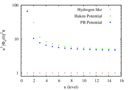
Figure 2: Oscillator strengths of polaron excitons and hydrogenic exciton.

The values of $\Phi(0)$ in Table 2 and Figure 2 shows that the ground exciton is optically active. According to Eq. (9) the oscillator strength in the PB model is 0.013. The second exciton level is only $2.7$ meV (Haken) or $1.2$ meV (PB) below the edge of the continuum spectrum, and their oscillator strengths are one order of magnitude smaller than for the main line ($n=1$), making these transitions practically undetectable in the optical spectra. Higher energies approach to the sequence $E_{g}-Ry_{0}/n^{2}$. For these higher levels, the oscillator strengths become proportional to the hydrogenic oscillator strengths. The proportionality constant is fitted to $\beta_{H}=4.282$ (Haken) and $\beta_{PB}=4.214$ (PB) in each case. The fitting function was $f(n)=\beta+\gamma/(n-n_{0})$, and the fitted $\beta$ are stable for any subset of data with $n>7$. Let us note that

$$\beta\simeq\frac{\epsilon_{0}}{\epsilon_{\infty}}.$$ (10)

This result, together with the approximation of the energies by the sequence $E_{g}^{*}-Ry_{0}/n^{2}$, leads to to a constant absorption spectrum near the band gap energy similar to the case of hydrogenic excitonGrosso and Pastori-Parravicini (2000); Elliot (1957),

$$\alpha(E_{g}^{*})=\frac{2\pi e^{2}\hbar P_{cv}^{2}}{E_{g}n_{r}cm_{0}^{2}}\frac{\beta}{a_{0}^{3}Ry_{0}},$$ (11)

where $n_{r}$ is the refraction index and can be approximated by $\sqrt{\epsilon_{\infty}}$. Evaluation the physical constants, and using Eqs. (10), (8), and (17), the above expression can be cast as

$$\alpha(E_{g}^{*})=(3.466\mbox{ nm}^{-1})\frac{U_{cv}}{n_{r}E_{g}}\left(\frac{\mu}{m_{0}}\right)^{2}\frac{1}{\epsilon_{\infty}},$$ (12)

Using the material parameters of CH₃NH₃PbI₃, $\alpha(E_{g})\sim 3.1$ $\mu$m^-1.

The exciton spectrum obtained presents of a low energy non-hydrogenic state that is 37 or 24 meV (in Haken or PB models, respectively) below the onset of continuous free polaron spectrum. The rest of the discrete exciton spectrum resembles the hydrogenic series with static dielectric constant $\epsilon_{0}$. The first exciton state dominates the absorption edge with oscillator strength $\sim 0.013$, while the oscillator strengths of higher states are one or two orders of magnitude smaller. Like the case of hydrogenic exciton, the coalescence of absorption lines from higher states generates a quasi-continuum spectrum with a finite value at the gap energy. The absorption coefficient at gap energy in enhanced with respect to the hydrogenic model by a factor $\epsilon_{0}/\epsilon_{\infty}$. Extrapolating this behavior to the room temperature tetragonal phase, this enhancement factor could be responsible of the high capacity of this material to collect the photon energy in the photovoltaic cells.

To interpret the absorption experiments and to determine de band gap, one needs to know wether the onset of the continuous absorption spectrum corresponds to the exciton continuum spectrum, or to the accumulation of discrete lines below the band gap. In other words, what is the energy range of constant absorption coefficient given by Eq. (12). Considering that the higher exciton levels are within 2 meV of the continuum, and that the exciton absorption spectrum is dominated by the fundamental state, one can conclude that the band gap coincides with the absorption threshold after filtering the first exciton peak. On the other hand, the polaronic effect downshifts the gap by 95 meV. Therefore, the measured gap 1.68 eV should be understood as an electronic gap of 1.78 eV decreased by the polaron shift.

Several kinds of estimations of the exciton binding energy in CH₃NH₃PbI₃ have been reported. The first method was employed by Hirasawa et alHirasawa et al. (1994), and repeated later with improved accuracy by Tanaka et alTanaka et al. (2003). They measured the exciton diamagnetic coefficient in magneto-absorption spectra, and related the measurements with the binding energy in the framework of the hydrogenic model with the high frequency dielectric constant. With this model, Tanaka et al determined a binding energy of 50 meV. The use of the high frequency dielectric constants was a choice of the model, and not determined by the experiments. Let us note that Tanaka et al, and Hirasawa et al used a value $\epsilon_{\infty}=6.5$ that is higher than our value. If our value $\epsilon_{\infty}=5.32$ were used, a binding energy of 65 meV would be obtained. Conversely, our binding energies using the larger dielectric constant would be smaller. These values of the exciton binding energy are strongly biased by the choice of the dielectric constants.

The second method has been applied by Sun et alSun et al. (2014) ($E_{B}=19$ meV). They obtained the binding energy by fitting the photoluminescence intensity as a function of temperature with an Arrhenius equation, not using any model of the exciton states. It is rewarding that our calculation of the binding energy is in good agreement with the values determined by Sun et al. Huang and LambrechtHuang and Lambrecht (2013) have argued, in a study of cesium tin halide perovskites, that the photoluminescence temperature dependence just give information on the free exciton linewidth or the binding energies of bound excitons, but not on free excitons. However, Even et alEven et al. (2014) fitted the absorption spectrum using the Wannier-Mott exciton model and obtained a similar value for the binding energy, and reported an effective dielectric constant $\epsilon_{eff}=11$. This value of the dielectric constants, together with the assumed reduced mass $0.16m_{0}$Even et al. (2014) means a binding energy of 19 meV. Another method independent of the dielectric function has been used by Miyata et alMiyata et al. (2015), who performed magneto-absorption experiments with very high magnetic fields, determining a value of $16\pm 2$ eV. It is interesting that Miyata et al were able to detect the $2s$ exciton state for high magnetic field and extrapolated a $1s-2s$ difference of 15 meV at low magnetic field. Henceforth, assuming the hydrogenic model, they estimated the binding energy in $20$ meV. However, extrapolating the Landau levels of the free exciton spectrum they obtained the precise value of $16$ meV. This observation agrees with our result that the $2s$ state is within $2$ meV of the free exciton edge.

The evaluation of the oscillator strength provides another argument against the model of hydrogenic Wannier excitons screened by $\epsilon_{0}$. IshiharaIshihara (1994) reported an experimental values of 0.02, which is close to our value 0.013. If the ground exciton were well described by hidrogenic model with $\epsilon_{0}$, then $\Phi_{1}(0)=1/\sqrt{\pi}$ (compare with Table 2 and Fig. 2), and the oscillator strength would be $\sim 64$ times smaller. Therefore, at least for low temperature, the fundamental exciton state does not correspond to screening by $\epsilon_{0}$.

We wish to stress that we have not fitted any parameter in this work, which would bring the exciton binding energies in closer agreement with the recent experimental results. The parameters with larger uncertainty are the dielectric constants and the LO phonon energy. The only available experimental value of $\epsilon_{\infty}=6.5$Hirasawa et al. (1994) is larger than the ab initio value used here and that value would reduce the calculated binding energy. The measurement of $\epsilon_{\infty}$ is rather old, with few published details, and a new determination for present-day thin films would be welcomed. The LO phonon energy $E_{LO}$ has been chosen from the more prominent peak in the calculated Raman spectrum of CH₃NH₃PbI₃Quarti et al. (2014), which is close to LO phonon energies in II-VI and III-V semiconductors. As mentioned above, the model Hamiltonians were developed assuming a unique LO phonon energy. The Raman spectrum of CH₃NH₃PbI₃ shows bands at lower wave numbers. Using and average energy of the Raman active peaks, which do not have necessarily LO character, may lead to lower exciton binding energy. An extension of the PB Hamiltonian to include several LO phonon branches would be a better founded approach.

In summary, we have calculated the exciton binding energies and oscillator strengths using two model Hamiltonians of the exciton-phonon coupled system. The Pollmann-Büttner model Hamiltonian gives a binding energy in good agreement with recent experimental determinations. The calculated oscillator strength of the main exciton line agrees with the value estimated from experiments, while the strengths of higher transitions are much smaller.

Appendix A Interband matrix element

With the VASP codeKresse and Furthmüller (1996) the tensor dielectric function is computed in the longitudinal approximationGajdoš et al. (2006)

$$\varepsilon^{(2)}_{\alpha\beta}(\omega) = \frac{4\pi^{2}e^{2}}{\Omega}\lim_{q\rightarrow 0}\frac{1}{q^{2}}\sum_{c,v,\mathbf{k}}g_{S}w_{\mathbf{k}}\delta(\epsilon_{c\mathbf{k+q}}-\epsilon_{v\mathbf{k}}-\hbar\omega)$$ (13)

$$\times\langle u_{c\mathbf{k}+\mathbf{e}_{\alpha}q}|u_{v\mathbf{k}}\rangle\langle u_{c\mathbf{k}+\mathbf{e}_{\beta}q}|u_{v\mathbf{k}}\rangle^{*},$$

where $w_{k}$ are the k-point weights, defined such that they sum to 1, $\epsilon_{c\mathbf{k+q}}$ are band energies, $\Omega$ is the unit cell volume, $m_{0}$ is the vacuum electron mass, $\mathbf{e}_{\alpha}$ are polarization vectors. The factor $g_{S}$ is the spin degeneracy, which is 2 in Ref. Gajdoš et al., 2006, and the bands $v,c$ in the sum are restricted to have the same spin. In the calculation with spin-orbit coupling, we consider $g_{S}=1$ and the sum is over all pairs of valence and conduction bands. The Eq. 13 is equivalent to the transverse approximationDel Sole and Girlanda (1993),

$$\varepsilon^{(2)}_{\alpha\beta}(\omega)=\frac{4\pi^{2}e^{2}}{\Omega\omega^{2}}\sum_{c,v,\mathbf{k}}g_{S}w_{\mathbf{k}}\delta(\epsilon_{c\mathbf{k}}-\epsilon_{v\mathbf{k}}-\hbar\omega)$$ (14)

$$\times \langle u_{c\mathbf{k}}|\hat{v}_{\alpha}+\frac{\hbar k_{\alpha}}{m_{0}}|u_{v\mathbf{k}}\rangle\langle u_{c\mathbf{k}}|\hat{v}_{\beta}+\frac{\hbar k_{\beta}}{m_{0}}|u_{v\mathbf{k}}\rangle^{*}.$$

For a local Hamiltonians with spin-orbit coupling, $m_{0}\hat{\vec{v}}=-i\hbar\nabla+(\hbar/4m_{0}c^{2})\vec{\sigma}\times\nabla V$. The PAW potentials and the hybrid functionals introduce non-locality in the Hamiltonian, and the velocity operator contains additional termsDel Sole and Girlanda (1993). For the purpose of the optical properties of the exciton, we only need the values of $\langle u_{c\mathbf{k}}|\hat{v}_{\beta}|u_{v\mathbf{k}}\rangle$ between the VBM and the CBM, which occurs at the $\Gamma$ point ($k_{\beta}=0$). These values $\langle u_{c\mathbf{k}}|\hat{v}_{\beta}|u_{v\mathbf{k}}\rangle$ can be fitted from the dielectric function, which is calculated using (13). Hence, if the contribution of the $\Gamma$ point can be separated from the other k-point contributions, we have that

$$\varepsilon^{(2)}_{\alpha\beta;\Gamma}(\omega) = \frac{4\pi^{2}e^{2}}{\Omega\omega^{2}}g_{S}w_{0}\sum_{cv}^{\prime}\delta(\epsilon_{c\mathbf{0}}-\epsilon_{v\mathbf{0}}-\hbar\omega)$$ (15)

$$\times\langle u_{c\mathbf{0}}|\hat{v}_{\alpha}|u_{v\mathbf{0}}\rangle\langle u_{c\mathbf{0}}|\hat{v}_{\beta}|u_{v\mathbf{0}}\rangle^{*}.$$

In the above expression, the sum $\sum^{\prime}$ is restricted to the top valence bands and bottom valence bands.

To fit with the exciton, we consider the averaged dielectric function $\varepsilon=(1/3)\mbox{Tr}\varepsilon_{\alpha\alpha}$

$$\varepsilon^{(2)}_{\Gamma}(\omega)=\frac{4\pi^{2}e^{2}}{\Omega\omega^{2}m_{0}^{2}}g_{S}w_{0}P_{cv}^{2}\delta(\epsilon_{c\mathbf{0}}-\epsilon_{v\mathbf{0}}-\hbar\omega),$$ (16)

with

$$P_{cv}^{2}=\frac{1}{3}\sum_{\alpha}\sum_{cv}^{\prime}|\langle u_{c\mathbf{0}}|m_{0}\hat{v}_{\alpha}|u_{v\mathbf{0}}\rangle|^{2}.$$ (17)

The parameter $P_{cv}$ has dimension of momentum, and $P_{cv}^{2}/2m_{0}$ is the parameter $U_{cv}$ defined in Eq. (8).

In practical calculations, $\delta(\epsilon_{c\mathbf{0}}-\epsilon_{v\mathbf{0}}-\hbar\omega)$ is replaced by a smearing function. If gaussian smearing is used for the self-consistent calculation, the computed spectrum must be fitted with a Gaussian function weighted by $4\pi^{2}e^{2}g_{S}w_{0}P_{cv}^{2}/\Omega\omega^{2}m_{0}^{2}$. The ab initio calculation was performed sampling the Brillouin zone with a $2\times 2\times 2$ k-point grid centered at the $\Gamma$ point, which is sufficient to obtain total energies and charge densities, but it is coarse for calculation of optical properties and it allows to isolate the contributions of the $\Gamma-$point transitions. With this k-point mesh, the weight $w_{0}=1/8$. The details of the calculation are given in Ref. Menéndez-Proupin et al., 2014.

References

- Kojima et al. (2009) A. Kojima, K. Teshima, Y. Shirai, and T. Miyasaka, J. Am. Chem. Soc. 131, 6050 (2009).
- nre (2015) (2015), NREL chart on record cell efficiencies, URL http://www.nrel.gov/ncpv/images/efficiency_chart.jpg.
- Jacoby (2014) M. Jacoby, Chemical & Engineering News 92, 21 (2014).
- Etgar et al. (2012) L. Etgar, P. Gao, Z. Xue, Q. Peng, A. K. Chandiran, B. Liu, M. K. Nazeeruddin, and M. Grätzel, J. Am. Chem. Soc. 134, 17396 (2012).
- Park (2013) N.-G. Park, J. Phys. Chem. Lett. 4, 2423 (2013).
- Knop et al. (1990) O. Knop, R. E. Wasylishen, M. A. White, T. S. Cameron, and M. J. M. van Ooort, Can. J. Chem. 68, 412 (1990).
- Baikie et al. (2013) T. Baikie, Y. Fang, J. M. Kadro, M. Schreyer, F. Wei, S. G. Mhaisalkar, M. Graetzel, and T. J. White, J. Mater. Chem. A 1, 5628 (2013).
- Stoumpos et al. (2013) C. C. Stoumpos, C. D. Malliakas, and M. G. Kanatzidis, Inorganic Chemistry 52, 9019 (2013).
- Kawamura et al. (2002) Y. Kawamura, H. Mashiyama, and K. Hasebe, J. Phys. Soc. Jpn. 71, 1694 (2002).
- Wasylishen et al. (1985) R. E. Wasylishen, O. Knopp, and J. B. Macdonald, Solid State Commun. 56, 581 (1985).
- Lin et al. (2015) Q. Lin, A. Armin, R. C. R. Nagiri, P. L. Burn, and P. Meredith, Nature Phot. 9, 106 (2015).
- Frost et al. (2014) J. M. Frost, K. T. Butler, and A. Walsh, APL Materials 2, 081506 (2014).
- Umari et al. (2014) P. Umari, E. Mosconi, and F. De Angelis, Sci. Rep. 4, 4467 (2014).
- Brivio et al. (2014) F. Brivio, K. T. Butler, A. Walsh, and M. van Schilfgaarde, Phys. Rev. B 89, 155204 (2014).
- Menéndez-Proupin et al. (2014) E. Menéndez-Proupin, P. Palacios, P. Wahnón, and J. C. Conesa, Phys. Rev. B 90, 045207 (2014).
- Ishihara (1994) T. Ishihara, J. Lumin. 60&61, 269 (1994).
- Hirasawa et al. (1994) M. Hirasawa, T. Ishihara, T. Goto, K. Uchida, and N. Miura, Physica B 201, 427 (1994).
- Tanaka et al. (2003) K. Tanaka, T. Takahashi, T. Ban, T. Kondo, K. Uchida, and N. Miura, Solid State Commun. 127, 619 (2003).
- D’Innocenzo et al. (2014) V. D’Innocenzo, G. Grancini, M. J. P. Alcocer, A. R. S. Kandada, S. D. Stranks, M. M. Lee, G. Lanzani, H. J. Snaith, and A. Petrozza, Nat. Commun. 5, 3586 (2014).
- Wannier (1937) G. Wannier, Phys. Rev. 52, 191 (1937).
- Knox (1963) R. Knox, Theory of excitons, Solid State Physics: Supplement 5 (Academic Press, 1963).
- Brivio et al. (2013) F. Brivio, A. B. Walker, and A. Walsh, APL Materials 1, 042111 (pages 5) (2013).
- Sun et al. (2014) S. Sun, T. Salim, N. Mathews, M. Duchamp, C. Boothroyd, G. Xing, T. C. Sumbce, and Y. M. Lam, Energy Environ. Sci. 7, 399 (2014).
- Even et al. (2014) J. Even, L. Pedesseau, and C. Katan, J. Phys. Chem. C 118, 11566 (2014).
- Miyata et al. (2015) A. Miyata, A. Mitiouglu, P. Plochocka, O. Portugall, J. T.-W. Wang, S. D. Stranks, H. J. Snaith, and R. J. Nicholas, Nature Phys. (2015), doi:10.1038/nphys3357, eprint arXiv:1504.07025.
- Haken (1956a) H. Haken, Z. Phys. 146, 527 (1956a), ISSN 0044-3328.
- Haken (1958) H. Haken, Fortschr. Phys. 6, 271 (1958).
- Pollmann and Büttner (1977) J. Pollmann and H. Büttner, Phys. Rev. B 16, 4480 (1977).
- Quarti et al. (2014) C. Quarti, G. Grancini, E. Mosconi, P. Bruno, J. M. Ball, M. M. Lee, H. J. Snaith, A. Petrozza, and F. De Angelis, J. Phys. Chem. Lett. 5, 279 (2014).
- Devreese and Alexandrov (2009) J. T. Devreese and A. S. Alexandrov, Rep. Prog. Phys. 72, 066501 (pages 55) (2009).
- Haken (1956b) H. Haken, J. Phys. Radium 17, 826 (1956b).
- Del Sole and Girlanda (1993) R. Del Sole and R. Girlanda, Phys. Rev. B 48, 11789 (1993).
- Grosso and Pastori-Parravicini (2000) G. Grosso and G. Pastori-Parravicini, Solid State Physics (Academic Press, San Diego, 2000), 1st ed.
- Elliot (1957) R. J. Elliot, Phys. Rev. 108, 1384 (1957).
- Huang and Lambrecht (2013) L.-Y. Huang and W. R. L. Lambrecht, Phys. Rev. B 88, 165203 (2013).
- Kresse and Furthmüller (1996) G. Kresse and J. Furthmüller, Phys. Rev. B 54, 11169 (1996).
- Gajdoš et al. (2006) M. Gajdoš, K. Hummer, G. Kresse, J. Furthmüller, and F. Bechstedt, Phys. Rev. B 73, 045112 (2006).