Scaling limits of a model for selection at two scales

Abstract

The dynamics of a population undergoing selection is a central topic in evolutionary biology. This question is particularly intriguing in the case where selective forces act in opposing directions at two population scales. For example, a fast-replicating virus strain out-competes slower-replicating strains at the within-host scale. However, if the fast-replicating strain causes host morbidity and is less frequently transmitted, it can be outcompeted by slower-replicating strains at the between-host scale. Here we consider a stochastic ball-and-urn process which models this type of phenomenon. We prove the weak convergence of this process under two natural scalings. The first scaling leads to a deterministic nonlinear integro-partial differential equation on the interval $[0,1]$ with dependence on a single parameter, $\lambda$. We show that the fixed points of this differential equation are Beta distributions and that their stability depends on $\lambda$ and the behavior of the initial data around $1$. The second scaling leads to a measure-valued Fleming-Viot process, an infinite dimensional stochastic process that is frequently associated with a population genetics.

1. Introduction

We study the model, introduced in [13], of a trait that is advantageous at a local or individual level but disadvantageous at a larger scale or group level. For example, an infectious virus strain that replicates rapidly within its host will outcompete other virus strains in the host. However, if infection with a heavy viral load is incapacitating and prevents the host from transmitting the virus, the rapidly replicating strain may not be as prevalent in the overall host population as a slow replicating strain.

A simple mathematical formulation of this phenomenon is as follows. Consider a population of $m\in\mathbb{N}$ groups. Each group contains $n\in\mathbb{N}$ individuals. There are two types of individuals: type I individuals are selectively advantageous at the individual (I) level and type G individuals are selectively advantageous at the group (G) level. Replication and selection occur concurrently at the individual and group level according to the Moran process [6] and are illustrated in Fig 1. Type I individuals replicate at rate $1+s$, $s\geq 0$ and type G individuals at rate $1$. When an individual gives birth, another individual in the same group is selected uniformly at random to die. To reflect the antagonism at the higher level of selection, groups replicate at a rate which increases with the number of type G indivduals they contain. As a simple case, we take this rate to be $w(1+r\frac{k}{n})$, where $\frac{k}{n}$ is the fraction of indivduals in the group that are type G, $r\geq 0$ is the selection coefficient at the group level, and $w>0$ is the ratio of the rate of group-level events to the rate of individual-level events. More general functions for the group replication rate are possible, though the subsequent analysis of the model may be less tractable. As with the individual level, the population of groups is maintained at $m$ by selecting a group uniformly at random to die whenever a group replicates. The offspring of groups are assumed to be identical to their parent.

As illustrated in Fig 1, this two-level process is equivalent to a ball-and-urn or particle process, where each particle represents a group and its position corresponds to the number of type G individuals that are in it.

Let $X_{t}^{i}$ be the number of type G individuals in group $i$ at time $t$. Then

$$\mu^{m,n}_{t}:=\frac{1}{m}\sum_{i=1}^{m}\delta_{X^{i}_{t}/n}$$

is the empirical measure at time $t$ for a given number of groups $m$ and individuals per group $n$. $\delta_{x}(y)=1$ if $x=y$ and zero otherwise. The $X^{i}_{t}$ are divided by $n$ so that $\mu^{m,n}_{t}$ is a probability measure on $E_{n}:=\{0,\frac{1}{n},\ldots,1\}$.

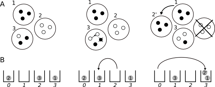
Figure 1. Schematic of the particle process. (a) Left: A population of $m=3$ groups, each with $n=3$ individuals of either type G (filled small circles) or type I (open small circles). Middle: A type I individual replicates in group 3 and a type G individual is chosen uniformly at random from group 3 to die. Right: Group 1 replicates and produces group $2^{\prime}$. Group 2 is chosen uniformly at random to die. (b) The states in (a) mapped to a particle process. Left: Group 2 has no type G individuals, represented by ball 2 in urn 0. Similarly, group 3 is represented by ball 3 in urn 2 and group 1 by ball 1 in urn 3. Middle: The number of type G individuals in group 3 decreases from two to one, therefore ball 3 moves to urn 1. Right: A group with zero type G individuals dies, while a group with three type G individuals is born. Therefore ball 2 leaves urn 0 and appears in urn 3 as ball $2^{\prime}$.

For fixed $T>0$, $\mu^{m,n}_{t}\in D([0,T],\mathcal{P}(E_{n}))$, the set of càdlàg processes on $[0,T]$ taking values in $\mathcal{P}(E_{n})$, where $\mathcal{P}(S)$ is the set of probability measures on a set $S$. With the particle process described above, $\mu^{m,n}_{t}$ has generator

(1) $$({L}^{m,n}\psi)(v)=\sum_{i,j}({R_{1}+wR_{2}})(v,v_{ij})[\psi(v_{ij})-\psi(v)]$$

where $v_{ij}:=v+\tfrac{1}{m}(\delta_{\frac{j}{n}}-\delta_{\frac{i}{n}})$, $\psi\in C_{b}(\mathcal{P}([0,1]))$ are bounded continuous functions, and $v\in\mathcal{P}(E_{n})\subset\mathcal{P}([0,1])$. The transition rates $({R_{1}+wR_{2}})$ are given by

$${R_{1}}\left(v,v_{ij}\right)=\left\{\begin{array}[]{lr}mv(\tfrac{i}{n})i\left(1-\tfrac{i}{n}\right)(1+s)&\text{ if }j=i-1,i<n\\ mv(\tfrac{i}{n})i\left(1-\tfrac{i}{n}\right)&\text{ if }j=i+1,i>0\\ 0&\text{ otherwise }\end{array}\right.$$

and

$${R_{2}}\left(v,v_{ij}\right)=mv(\tfrac{i}{n})v(\tfrac{j}{n})(1+r\tfrac{j}{n}).$$

$R_{1}$ represents individual-level events while $R_{2}$ represents group-level events.

Acknowledgements: The authors would like to thank Mike Reed and Katia Koelle for their roles in the collaboration out of which this paper’s central model grew. We would also like to thank Rick Durrett of a number of useful discussions. JCM would like to thank the NSF for its support though DMS-08-54879. SL would like to thank support from the NSF (grants NSF-EF-08-27416 and DMS-0942760), NIH (grant R01-GM094402), and the Simons Institute for the Theory of Computing.

2. Main results

We prove the weak convergence of this measure-valued process as $m,n\to\infty$ under two natural scalings. The first scaling leads to a deterministic partial differential equation. We derive a closed-form expression for the solution of this equation and study its steady-state behavior. The second scaling leads to an infinite dimensional stochastic process, namely a Fleming-Viot process.

Let us briefly introduce some notation. By $m,n\to\infty$ we mean a sequence $\{(m_{k},n_{k})\}_{k}$ such that for any $N$, there is an $n_{0}$ such that if $k\geq n_{0}$, $m_{k},n_{k}\geq N$. We define $\langle f,v\rangle=\int_{0}^{1}f(x)v(dx)$ where $f$ is a test function and $v$ a measure. Lastly, $\delta_{x}$ will denote the delta measure for both continuous and discrete state spaces.

To provide intuition for the two scalings and the corresponding limits, take $\psi$ to be of the form $\psi(v)=F(\langle g,v\rangle)$, where $g$ is some suitable function on $[0,1]$, and apply the generator in (1) to it:

$$L^{m,n}\psi(\mu) =F^{\prime}\cdot\Big{\{}\sum\left[\tfrac{1}{n}g^{\prime\prime}(\tfrac{i}{n})-sg^{\prime}(\tfrac{i}{n})\right]\tfrac{i}{n}(1-\tfrac{i}{n})\mu(\tfrac{i}{n})$$

$$\qquad\qquad+wr\left[\sum\tfrac{i}{n}g(\tfrac{i}{n})\mu(\tfrac{i}{n})-\sum g(\tfrac{i}{n})\mu(\tfrac{i}{n})\sum\tfrac{j}{n}\mu(\tfrac{j}{n})\right]\Big{\}}$$

$$\qquad+\tfrac{1}{m}wF^{\prime\prime}\cdot\Big{\{}\sum g(\tfrac{i}{n})^{2}\mu(\tfrac{i}{n})-\left(\sum g(\tfrac{i}{n})\mu(\tfrac{i}{n})\right)^{2}$$

$$\qquad\qquad\qquad\qquad+\tfrac{1}{2}r\sum(g(\tfrac{j}{n})-g(\tfrac{i}{n})^{2}\tfrac{j}{n}\mu(\tfrac{j}{n})\mu(\tfrac{i}{n})\Big{\}}$$

$$\qquad+o(\tfrac{1}{m})+o(\tfrac{1}{n})$$

This suggests two natural scalings. The first is to take $m,n\to\infty$ without rescaling any parameters. The $g^{\prime\prime}$ and $F^{\prime\prime}$ terms vanish and we have a deterministic process. The precise statement of the weak convergence of the finite state space system to the deterministic limit is in terms of a weak measure-valued solution to a partial differential equation:

Theorem 1.

Suppose the particles in the system described by $\mu^{m,n}_{t}$ are initially independently and identically distributed according to the measure $\mu^{m,n}_{0}$, where $\mu^{m,n}_{0}\to\mu_{0}\in\mathcal{P}([0,1])$ as $m,n\to\infty$. Then, as $m,n\to\infty$, $\mu^{m,n}_{t}\to\mu_{t}\in D([0,T],\mathcal{P}([0,1]))$ weakly, where $\mu_{t}$ solves the differential equation

(2) $$\tfrac{d}{dt}\langle f,\mu_{t}\rangle=-\langle x(1-x)f^{\prime},\mu_{t}\rangle+\lambda\left[\langle xf,\mu_{t}\rangle-\langle f,\mu_{t}\rangle\langle x,\mu_{t}\rangle\right]$$

for any positive-valued test function $f\in C^{1}([0,1])$ and with initial condition $\langle f,\mu_{0}\rangle$. Here, $\lambda:=\frac{wr}{s}$ and time has been sped up by a factor of $s$.

Throughout we will denote the measure-valued solutions to (2) by $\mu_{t}(dx)$. We note that strong, density-valued solutions, denoted by $\eta_{t}(x)$, solve:

(3) $$\tfrac{\partial}{\partial t}\eta_{t}=\tfrac{\partial}{\partial x}\left[x(1-x)\eta_{t}\right]+\lambda\eta_{t}\cdot\left(x-\int_{0}^{1}y\eta_{t}(y)dy\right)$$

with initial density $\eta_{0}(x)$. In this more transparent form one can see that the first term on the right is a flux term that transports density towards $x=0$ whereas the second term is a forcing term that increases the density at values of $x$ above the mean of the density. The flux corresponds to the individual-level moves: nearest neighbor moves in the particle system. The forcing term corresponds to group-level moves: moves to occupied sites in the particle system.

We will see that if we start with an initial measure $\mu_{0}$ which is the sum of delta measures, then the solution $\mu_{t}$ retains the same form. More explicitly, if

$$\mu_{0}(dx)=\sum_{i}a_{i}(0)\delta_{x_{i}(0)}(dx)$$

where $x_{i}(0)\in[0,1]$, $a_{i}(0)>0$, and $\sum a_{i}(0)=1$, then we will see (from Lemma 5) that the solution $\mu_{t}$ to (2) has the form

$$\mu_{t}(dx)=\sum_{i}a_{i}(t)\delta_{x_{i}(t)}(dx)\,.$$

Moreover, the parameters $(a_{i}(t),x_{i}(t))$ satisfy the following set of coupled equations

(4) $$\left\{\begin{aligned} \frac{dx_{i}}{dt}&=-x_{i}(1-x_{i})\\ \frac{da_{i}}{dt}&=\lambda a_{i}\Big{(}x_{i}-\langle y,\mu_{t}\rangle\Big{)}=\lambda a_{i}\Big{(}x_{i}-\sum_{j}a_{j}x_{j}\Big{)}\,.\end{aligned}\right.$$

Notice that the positions of the delta masses change according to a negative logistic function, independently of the other masses and the density. The weight $a_{i}$ increases at time $t$ if the position of the particle $x_{i}$ is above the mean, $\sum a_{j}x_{j}$, and decreases if it is below the mean. To build intuition, it is instructive to consider some simple examples of this form.

Example 1.

According to (4), if $\mu_{0}=\delta_{1}$, then $\mu_{t}=\mu_{0}$. This can also be seen directly from (2). In the case of an initial condition containing some delta mass at $1$, all of the rest of the mass will migrate towards zero. Eventually all of the mass will be below the mean as the mass at one will not move and will ever be increasing its mass as it is always above the mean. Once this happens it is clear that all of the mass will drain from all of the points not at one and hence $\mu_{t}\rightarrow\delta_{1}$ as $t\rightarrow\infty$. This reasoning holds in a more general setting and is included in Theorem 3.

Example 2.

According to (4), if $\mu_{0}=\delta_{0}$, then $\mu_{t}=\mu_{0}$. This too can be seen directly from (2). In the case of an initial condition containing no mass at one and only finite number of masses total, the mass will eventually all move towards zero and hence hence $\mu_{t}\rightarrow\delta_{0}$ as $t\rightarrow\infty$. If an infinite number of masses are allowed the situation is not as simple. Theorem 3 hints at the possible complications by giving an example of a density which is invariant.

Though $\delta_{0}$ is a fixed point of the system attracting many initial configurations, it is not Lyapunov stable. This means that even small perturbations of $\delta_{0}$ can lead to an arbitrary large excursion away from $\delta_{0}$ even though the system eventually returns to $\delta_{0}$. Rather than making a precise statement which would require quantifying the size of a perturbation, consider the example of $\mu_{0}=(1-\varepsilon)\delta_{0}+\varepsilon\delta_{1-\alpha}$. As $\varepsilon\rightarrow 0$, the distance between $\mu_{0}$ and $\delta_{0}$ goes to zero in any reasonable metric. If we write $\mu_{t}=(1-a_{t})\delta_{0}+a_{t}\delta_{x_{t}}$ then as $\alpha\rightarrow 0$ one can ensure that the system spends arbitrarily long time with $x_{t}>\frac{1}{2}$ and hence $a_{t}$ will grow to as close to one as one wants in this time. Thus the system could be described as making an an arbitrarily big excursion away from $\delta_{0}$ even though $\mu_{t}\rightarrow\delta_{0}$ as $t\rightarrow\infty$.

It natural to ask if there are other fixed points beyond $\delta_{0}$ and $\delta_{1}$.

Lemma 2 (Fixed points).

The measures delta $\delta_{0}$, $\delta_{1}$, and densities in the $Beta(\lambda-\alpha,\alpha)$ family of distributions:

$$\frac{1}{B(\lambda-\alpha,\alpha)}x^{\lambda-\alpha-1}(1-x)^{\alpha-1}$$

with $\alpha\in(0,\lambda)$, are fixed points of (2). $B(\lambda-\alpha,\alpha)$ is the normalizing constant that makes the density integrate to 1 over the interval $[0,1]$.

For measure-valued initial data, we show that the basins of attraction for the fixed points are determined by whether they charge the point $x=1$ and their Hölder exponent around $x=1$.

Theorem 3 (Steady state behavior).

Consider measure valued solution $\mu_{t}(dx)$ to (2) with initial probability measure $\mu_{0}(dx)$. If $\mu_{0}(\{1\})>0$ then

$$\mu_{t}\rightarrow\delta_{1}\qquad\text{as}\qquad t\rightarrow\infty$$

and if $\mu_{0}([1-\varepsilon,1])=0$ for some $\varepsilon>0$ then

$$\mu_{t}\rightarrow\delta_{0}\qquad\text{as}\qquad t\rightarrow\infty\,.$$

Alternatively, suppose that for some $\alpha>0$ and $C>0$

$$x^{-\alpha}\mu_{0}([1-x,1])\rightarrow C\qquad\text{as}\qquad x\rightarrow 0\,.$$

If $\alpha<\lambda$, then

$$\mu_{t}(dx)\rightarrow\text{Beta}(\lambda-\alpha,\alpha)\qquad\text{as}\qquad t\rightarrow\infty\,.$$

Otherwise, if $\alpha\geq\lambda$,

$$\mu_{t}(dx)\to\delta_{0}(dx)\qquad\text{as}\qquad t\to\infty$$

The results of Theorem 3 should be contrasted with the original Markov chain before taking the limit $m,n\rightarrow\infty$. In the Markov chain, all individuals eventually become either entirely type G or type I. These two homogeneous states are absorbing states for the individual level dynamics. The population level state made of individuals that are all either homogeneous of type G or I is absorbing for the group level dynamics. Hence, the state of the system eventually becomes composed entirely of homogeneous groups of solely G or I and stays in that state for all future times.

These two absorbing states of the Markov chain, with finite $m$ and $n$, correspond to the states $\delta_{0}$ and $\delta_{1}$ in the scaling limit. Hence the natural discretization for the Beta distribution to the lattice $\{\frac{k}{n}:0<k<n\}$, given by

$$\frac{1}{Z(m,n,\lambda,\alpha)}\big{(}\tfrac{k}{n}\big{)}^{\lambda-\alpha-1}\big{(}1-\tfrac{k}{n}\big{)}^{\alpha-1},$$

cannot be invariant. (Here $Z$ is the normalization constant which ensures the probabilities sum to one.) However for large $m$ and $n$, it is reasonable to expect it to be nearly invariant in the sense that if the initial states $\{X_{i}(0):1\leq i\leq m\}$ are independent and distributed as the discrete Beta distribution then the Markov chain dynamics will keep the distribution close to the product of discretized Beta distributions for a long time. The expectation of this time will grow to infinity as $m,n\rightarrow\infty$.

We will not pursue a rigorous proof of this near or quasi invariance here. Nonetheless, we now briefly sketch the argument as we understand it, giving the central points. If the distribution of the Markov chain is close to a product of discretized Beta distributions, then the empirical mean will be highly concentrated around the mean of continuous Beta when $m$ and $n$ are large. Hence the generator projected on to any $X_{i}$ is nearly decoupled from the other particles and close to being Markovian. More precisely, the dynamics of any fixed $X_{i}$ is well approximated in this setting by the one-dimensional Markov chain obtained by replacing the mean of the empirical measure in the full generator with the mean of the Beta distribution. It is straightforward to see that for $m$ and $n$ large the discretized Beta distribution is an approximate left-eigenfunction of this one-dimensional generator with an eigenvalue which goes to zero as $m,n\rightarrow\infty$.

All of these observations can be combined to show that if the systems starts in the product discretized Beta distribution then it will say close to the product discretized Beta distribution for a long time if $m$ and $n$ are large.

We now turn to the second scaling. Let $s=\frac{\sigma}{n}$, $r=\frac{\rho}{m}$, and $\frac{n}{m}\to\theta$, and let $\nu^{m,n}_{t}$ denote the empirical measure under this scaling. The terms $F^{\prime\prime}$ and $g^{\prime\prime}$ in the generator (1) no longer vanish and the process converges to a limit that is stochastic. Our weak convergence result is proved and stated in terms of a martingale problem.

Theorem 4.

Suppose $\frac{n}{m}\to\theta$, $w=O(1)$, $s=\tfrac{\sigma}{n}$, $r=\tfrac{\rho}{m}$, and we speed up time by a factor of $n$. Suppose the particles in the rescaled $\nu^{m,n}_{t}$ process are initially independently and identically distributed according to the measure $\nu^{m,n}_{0}$ where $\nu^{m,n}_{0}\to\nu_{0}$ as $m,n\to\infty$. Then the rescaled process converges weakly to $\nu_{t}$ as $m,n\to\infty$, where $\nu_{t}$ satisfies the following martingale problem:

(5) $$N_{t}(f) =\langle f,\nu_{t}\rangle-\langle f,\nu_{0}\rangle-\int_{0}^{t}\langle Af,\nu_{z}\rangle dz$$

$$\qquad-w\theta\rho\int_{0}^{t}\left\{\int_{0}^{1}\int_{0}^{1}f(x)V(z,\nu_{z},y)Q(\nu_{z};dx,dy)\right\}dz$$

is a martingale with conditional quadratic variation

(6) $$\langle N(f)\rangle_{t} =2w\theta\int_{0}^{t}\left[\int_{0}^{1}\int_{0}^{1}f(x)f(y)Q(\nu_{\tau};dx,dy)\right]d\tau$$

where

$$Af(x) =x(1-x)\left[\tfrac{d^{2}}{dx^{2}}f(x)-\sigma\tfrac{d}{dx}f(x)\right]$$

$$V(t,\nu,x) =x$$

$$Q(\nu;dx,dy) =\nu(dx)(\delta_{x}(dy)-\nu(dy))$$

and $f\in C^{2}([0,1])$.

The drift part of the martingale (5) comprises a second order partial differential operator $A$ and the centering term from the global jump dynamics (the expression in curly brackets). The entire process is a Fleming-Viot process [9]. Fleming-Viot processes frequently arise in models of population genetics (see [8] for a review). In these contexts, the variable $x$ can represent the geographical location of an individual, or as in the original paper of Fleming and Viot [9], the genotype of an individual (where genotype is a continuous instead of a discrete variable). To our knowledge, the specific form of the limiting Fleming-Viot process above has not previously been studied. In particular, although infinite dimensional stochastic processes have been applied to multilevel population dynamics of a single type [5], this appears to be the first Fleming-Viot process for the evolution of two types under opposing forces of selection at two population scales.

The dynamical properties of the deterministic partial differential equation (2) are the focus of the next section. The proofs of weak convergence (Theorems 1 and 4) are deferred to section 4.

3. Properties of the deterministic limit

We begin with a closed-form expression for solutions to the deterministic partial differential equation (2).

Lemma 5.

The solution to the deterministic partial differential equation (2) with initial measure $\mu_{0}$ is given by

(7) $$\mu_{t}(dx) =(G_{t}\mu_{0})(dx)=(\mu_{0}\phi^{-1}_{t})(dx)\cdot w_{t}(x)$$

where

$$\phi^{-1}_{t}(x)=\frac{x}{e^{-t}+x(1-e^{-t})}$$

$$w_{t}(x)=\left[(e^{-t}+x(1-e^{-t}))e^{t-\int_{0}^{t}h(z)dz}\right]^{\lambda}$$

and $h(t)$ satisfies $h(t)=\langle x,\mu_{t}\rangle$

Remark 1: $(\mu_{0}\phi^{-1}_{t})(dx):=\mu_{0}(\phi^{-1}_{t}(dx))$ captures the changes in the initial data that are solely due to the flux term. This expression is also known as the push-forward measure of $\mu_{0}$ under the dynamics of $\phi$. As we will see in the proof, $\phi_{t}(x)$ is precisely the characteristic curve for the spatial variable $x$ and includes a normalizing constant. The multiplication by $w_{t}(x)$ captures the changes in the initial data that are due to the forcing term in (2) and includes a normalizing factor.

Remark 2: Density-valued solutions are given by

$$\eta_{t}(x) =\eta_{0}(\phi_{t}^{-1}(x))\partial_{x}\phi_{t}^{-1}(x)\cdot w_{t}(x)$$

(8) $$=\eta_{0}\left(\tfrac{x}{e^{-t}+x(1-e^{-t})}\right)[e^{-t}+x(1-e^{-t})]^{\lambda-2}e^{(\lambda-1)t-\lambda\int_{0}^{t}h(z)dz}$$

To see this, suppose $\mu_{0}(dx)=\eta_{0}(x)dx$. Then for any test function $f$,

$$\int_{0}^{1}f(x)(\mu_{0}\phi^{-1}_{t})(dx)=\int_{0}^{1}(f\circ\phi_{t})(x)\mu_{0}(dx)=\int_{0}^{1}f(y)\eta_{0}(\phi_{t}^{-1}(y))\partial_{y}\phi_{t}^{-1}(y)dy$$

The first equality follows from the change-of-variable property of push-forward measures and the second from a standard change of variables. The limits of integration do not change because $0$ and $1$ are fixed points of both $\phi_{t}$ and $\phi_{t}^{-1}$.

Proof of Lemma 5.

We apply the method of characteristics (see for example [14]) to obtain a formula for a density-valued solution. We then prove that the weak, measure-valued analog of this solution satisfies (2). Consider the following modification of (3):

(9) $$\tfrac{\partial}{\partial t}\xi(t,x)=\tfrac{\partial}{\partial x}[x(1-x)\xi(t,x)]+\lambda\xi(t,x)\left[x-h(t)\right]$$

where $h(t)$ is a general function in time and $\xi_{0}\in C^{1}([0,1])$. Note that when $h(t)=\int_{0}^{1}y\xi(t,y)dy$, this differential equation is equivalent to (3). To be clear about which equation we are solving, we use $\xi(t,x)$ to denote solutions when $h(t)$ is unspecified.

Rewriting (9):

$$\left(\tfrac{\partial}{\partial t}\xi,\tfrac{\partial}{\partial x}\xi,-1\right)\cdot\left(1,-x(1-x),\left[(1-2x)+\lambda(x-h(t))\right]\xi\right) =0$$

The second vector is therefore tangent to the solution surface and gives the rates of change for the $t$, $x$, and $\xi$ coordinates. Let the initial condition be parameterized as $(0,x,\xi_{0}(x))=(0,p,\xi_{0}(p))$. The $t$, $x$, and $\xi$ coordinates change according to the characteristic equations

$$\tfrac{dt}{dq} =1 t(0,p)=0$$

$$\tfrac{dx}{dq} =-x(1-x) x(0,p)=p$$

$$\tfrac{d\xi}{dq} =\left[(1-2x(q,p))+\lambda(x(q,p)-h(t(q,p)))\right]\xi \xi(0,p)=\xi_{0}(p)$$

where $q$ is the parameter as we move through the solutions in time. The first two ordinary differential equations have solutions

$$t(q,p) =q$$

(10) $$x(q,p) =\frac{p}{p-(p-1)e^{q}}=:\phi_{q}(p)$$

From this, the third differential equation can be solved exactly:

$$\frac{d\xi}{dq} =\left[1+\tfrac{p}{p-(p-1)e^{q}}(\lambda-2)-\lambda h(q)\right]\xi$$

$$\xi(q,p) =\xi_{0}(p)\exp\left\{q-\lambda\int_{0}^{q}h(z)dz+(\lambda-2)\int_{0}^{q}\frac{p}{p-(p-1)e^{z}}~{}dz\right\}$$

$$=\xi_{0}(p)e^{q-\lambda\int_{0}^{q}h(z)dz}\left[p(e^{-q}-1)+1\right]^{(-\lambda+2)}$$

Next, make the substitutions $q=t$ and $p=\phi_{t}^{-1}(x)$ from (10) to obtain $\xi$ in terms of $t$ and $x$:

$$\xi(t,x) =(\xi_{0}\circ\phi_{t}^{-1})(x)\left[e^{-t}+x(1-e^{-t})\right]^{(\lambda-2)}e^{(\lambda-1)t-\lambda\int_{0}^{t}h(z)dz}$$

(11) $$=(\xi_{0}\circ\phi_{t}^{-1})(x)\partial_{x}\phi_{t}^{-1}(x)\cdot w_{t}(x)$$

If $h(t)$ satisfies $h(t)=\int_{0}^{1}y\xi(t,y)dy$, then by definition, $\xi(t,x)$ solves the partial differential equation (3). Conversely, if $\xi(t,x)$ solves the partial differential equation (3), it also solves the differential equation (9) with $h(t)=\int_{0}^{1}y\xi(t,y)dy$. Therefore this above expression, along with the condition $h(t)=\int_{0}^{1}y\xi(t,y)dy$, are equivalent to solutions of (3).

To extend this result to measures, suppose we have a strong solution $\eta_{t}(x)$ with initial condition $\eta_{0}$:

$$\eta_{t}(x)=(\eta_{0}\circ\phi_{t}^{-1})(x)\partial_{x}\phi_{t}^{-1}(x)\cdot w_{t}(x)$$

Using a similar calculation as that in Remark 2, the measure $\mu_{t}(dx)$ corresponding to $\eta_{t}(x)$ is given by

$$\mu_{t}(dx)=(\mu_{0}\phi_{t}^{-1})(dx)\cdot w_{t}(x)$$

It remains to check that this satisfies the weak deterministic partial differential equation (2), with $h(t)=\langle x,\mu_{t}\rangle$. The left hand side of the equation is

$$\tfrac{d}{dt}\langle f,\mu_{t}\rangle =\tfrac{d}{dt}\int_{0}^{1}f(x)w_{t}(x)(\mu_{0}\phi_{t}^{-1})(dx)=\tfrac{d}{dt}\int_{0}^{1}f(\phi_{t}(x))w_{t}(\phi_{t}(x))\mu_{0}(dx)$$

Differentiating under the integral sign, expanding out the expressions for $\partial_{t}\phi_{t}$ and $\partial_{t}(w_{t}(\phi_{t}(x))$, and applying change of variables for push-forward measures again, we obtain

$$\tfrac{d}{dt}\langle f,\mu_{t}\rangle ={-\int_{0}^{1}x(1-x)f^{\prime}(x)w_{t}(x)(\mu_{0}\phi_{t}^{-1})(dx)}+\lambda\int_{0}^{1}\left[x-h(t)\right]f(x)w_{t}(x)(\mu_{0}\phi_{t}^{-1})(dx)$$

This matches right hand side of the weak deterministic partial differential equation (2). ∎

In practice, the condition $h(t)=\langle x,\mu_{t}\rangle$ is difficult to use. The following provides an equivalent and simpler condition.

Lemma 6 (Conservation of measure condition).

Suppose $\xi$ is a weak measure-valued solution to the deterministic partial differential equation (9) with initial condition $\int_{0}^{1}\xi_{0}(dx)=1$. Then

$$h(t)=\int_{0}^{1}y\xi(t,dy)\qquad\text{ if and only if }\qquad\int_{0}^{1}\xi(t,dy)=1~{}\forall~{}t>0$$

Proof.

($\Rightarrow$ direction) Suppose $h(t)=\int_{0}^{1}y\xi(t,dy)$. Then $\xi$ is a weak measure-valued solution to (2). Taking the test function $f\equiv 1$, we obtain

$$\tfrac{d}{dt}\langle 1,\xi\rangle =0+\lambda[\langle x,\xi\rangle-\langle 1,\xi\rangle\langle x,\xi\rangle]=0$$

Thus, if the initial data has total measure $1$, $\langle 1,\xi\rangle$ remains constant at $1$ for all $t\geq 0$.

($\Leftarrow$ direction) Suppose $\int_{0}^{1}\xi(t,dx)=1$ for all $t>0$. Again take the test function $f\equiv 1$ but this time with unspecified $h(t)$:

$$0=\tfrac{d}{dt}\langle 1,\xi\rangle =0+\lambda[\langle x,\xi\rangle-\langle 1,\xi\rangle h(t)]=\lambda[\langle x,\xi\rangle-h(t)].$$

For this to hold, we must have $h(t)=\int_{0}^{1}x\xi(t,dx)$. ∎

The above lemmas imply that solutions $\mu_{t}(dx)$ to (2) can be obtained by using formula (7) from Lemma 5 and imposing the conservation of measure condition $\langle 1,\mu_{t}\rangle\equiv 1$ from Lemma 6. We illustrate this with some examples of exactly solvable solutions for special choices of initial data. We will see that the long time behavior of the examples is consistent with results stated in Theorem 3.

Example 3.

Initial measure concentrated at $x_{0}\in[0,1]$, i.e. $\mu_{0}=\delta_{x_{0}}$
Using formula (7),

$$\int f(x)\mu_{t}(dx) =\int f(x)w_{t}(x)\delta_{x_{0}}(\phi_{t}^{-1}(dx))=f(\phi_{t}(x_{0}))w_{t}(\phi_{t}(x_{0}))$$

$$=\int f(x)w_{t}(x)\delta_{\phi_{t}(x_{0})}(dx)$$

Thus $\mu_{t}(dx)=w_{t}(x)\delta_{\phi_{t}(x_{0})}(dx)$. Imposing the conservation of measure condition gives $\mu_{t}(dx)=\delta_{\phi_{t}(x_{0})}(dx)$. In other words, an initial delta measure at $x_{0}$ moves as a delta measure along the $x$ axis with position given by $\phi_{t}(x_{0})$, the solution to the negative logistic equation with initial position $x_{0}$.

Example 4.

Initial uniform density: $\eta_{0}(x)=1$, i.e $\mu_{0}(dx)=dx$
Using formula (8),

$$\eta_{t}(x) =e^{(\lambda-1)t-\lambda\int_{0}^{t}h(z)dz}\left[e^{-t}+x(1-e^{-t})\right]^{(\lambda-2)}$$

Imposing conservation of measure:

$$e^{(\lambda-1)t-\lambda\int_{0}^{t}h(z)dz} =\left[\int_{0}^{1}\left[e^{-t}+x(1-e^{-t})\right]^{(\lambda-2)}dx\right]^{-1}$$

$$=\begin{cases}\displaystyle\frac{(\lambda-1)(1-e^{-t})}{1-e^{-(\lambda-1)t}}&\text{if }\lambda\neq 1\\ \\ \displaystyle\frac{1-e^{-t}}{t}&\text{if }\lambda=1\end{cases}$$

Thus,

$$\eta_{t}(x) =\begin{cases}\displaystyle\frac{(\lambda-1)(1-e^{-t})}{1-e^{-(\lambda-1)t}}\left[e^{-t}+x(1-e^{-t})\right]^{(\lambda-2)}&\text{if }\lambda\neq 1\\ \\ \displaystyle\frac{1-e^{-t}}{t}\left[e^{-t}+x(1-e^{-t})\right]^{(\lambda-2)}&\text{if }\lambda=1\end{cases}$$

Note that $\eta_{0}\equiv 1$ corresponds to an initial condition satisfying the hypothesis of Theorem 3 with $\alpha=1$. As predicted when $\lambda>1$, we obtain $\eta(t,x)\to(\lambda-1)x^{\lambda-2}=\text{Beta}(\lambda-1,1)$ as $t\to\infty$.

The following is an example with $\alpha>1$.

Example 5.

If $\eta_{0}(x)=2(1-x)$, i.e. $\mu_{0}([1-x,1])=x^{2}$, then the corresponding $\alpha$ from Theorem 3 is $\alpha=2$.

Using formula (8)

$$\eta_{t}(x) =2e^{(\lambda-2)t-\lambda\int_{0}^{t}h(z)dz}(1-x)\left[e^{-t}+x(1-e^{-t})\right]^{(\lambda-3)}$$

Imposing the condition in Lemma 6 to solve for the $h(z)$ term

$$e^{(\lambda-2)t-\lambda\int_{0}^{t}h(z)dz}= \left[2\int_{0}^{1}(1-x)\left[e^{-t}+x(1-e^{-t})\right]^{(\lambda-3)}dx\right]^{-1}$$

$$= \begin{cases}\frac{(\lambda-2)(1-e^{-t})}{2}\left[\frac{1}{(\lambda-1)(1-e^{-t})}-\frac{e^{-(\lambda-1)t}}{(\lambda-1)(1-e^{-t})}-e^{-(\lambda-2)t}\right]^{-1}&\text{if }\lambda\neq 2\\ \frac{(1-e^{-t})^{2}}{2te^{-t}}&\text{if }\lambda=2\end{cases}$$

As predicted by Theorem 3 for $\lambda>2=\alpha$,

$$\eta_{t}(x)\to\tfrac{1}{2}(\lambda-2)(\lambda-1)(1-x)x^{\lambda-3}=\text{Beta}(\lambda-2,2)$$

as $t\to\infty$.

Example 6.

$\eta_{0}(x)=\frac{1}{c}\cdot 1_{[0,c]}(x)$ with $c<1$.

Using formula (8)

$$\eta_{t}(x)=\tfrac{1}{c}\mathbf{1}\{x\leq\phi_{t}(c)\}w_{t}(x)\partial_{x}\phi_{t}^{-1}(x)$$

Since $\phi_{t}(c)=\frac{ce^{-t}}{1-c+ce^{-t}}\to 0$ as $t\to\infty$, $\eta_{t}(x)\to 0$ for any $x>0$. Since $\eta$ must have total mass 1, it follows that regardless of the value of $\lambda$, $\eta_{t}(x)dx\to\delta_{0}(dx)\text{ for any }c<1$. This can also be seen by applying Theorem 3 and noting that $\mu_{0}([1-c,1])=\int_{1-c}^{1}\eta_{0}(x)dx=0$.

We end these examples with solutions for $\mu_{0}$ that are mixtures of delta measures and densities. First, note that it is straightforward to extend Example 3 to the case where $\mu_{0}(dx)=\sum a_{i}\delta_{x_{i}}(dx)$ is a linear combination of delta measures, $a_{i}>0$ for all $i$. Applying (7), we obtain

$$\mu(t,dx)=\sum_{i}a_{i}w_{t}(x)\delta_{\phi_{t}(x_{i})}(dx)=\sum_{i}a_{i}(t)\delta_{x_{i}(t)}(dx)$$

where $x_{i}(t)=\phi_{t}(x_{i})$ and $a_{i}(t)=a_{i}w_{t}(x)|_{x=x_{i}(t)}$. Our earlier system of equations (4) is obtained from this and the definitions of $\phi_{t}(x)$ and $w_{t}(x)$.

Second, we consider a combination of a delta measure and a density

$$\mu_{0}(dx)=a\delta_{x_{0}}(dx)+(1-a)v_{0}(x)dx$$

Notice that the formula for the solution (7) at first seems linear in the initial condition:

$$\int f(x)\mu_{t}(dx) =\int f(x)(G_{t}\mu_{0})(dx)$$

$$=\int f(x)w_{t}(x)[a\delta_{\phi_{t}(x_{0})}(dx)+(1-a)v_{0}(\phi^{-1}_{t}(x))\partial_{x}\phi^{-1}_{t}(x)dx]$$

$$=\int f(x)[a(G_{t}\delta_{x_{0}})(dx)+(1-a)(G_{t}v_{0})(dx)]$$

This gives $(G_{t}\mu_{0})(dx)=a(G_{t}\delta_{x_{0}})(dx)+(1-a)(G_{t}v_{0})(dx)$. However, this notation is misleading because implicit in the $G_{t}$ operator is the function $h(t)$, the mean of the overall process over time. Here, $h(t)$ involves both the delta measure and the density. The solution operator $G_{t}$ is therefore not linear for this reason.

Nevertheless, we can still use this formula to obtain expressions for solutions. We illustrate this with a concrete example.

Example 7.

Take $x_{0}=0$ and $v_{0}(x)$ the density function for $\text{Beta}(\lambda-\alpha,\alpha)$ with $\alpha\in(0,\lambda)$. Using the solution formula and direct calculation, we obtain

$$\mu_{t}(dx) =aw_{t}(0)\delta_{0}(dx)+(1-a)w_{t}(x)(v_{0}\circ\phi_{t}^{-1})(x)\partial_{x}\phi_{t}^{-1}(x)dx$$

$$=e^{-\lambda\int_{0}^{t}h(z)dz)}\left\{a\delta_{0}(dx)+(1-a)e^{(\lambda-\alpha)t}v_{0}(x)dx\right\}$$

Note in particular that $\mu_{t}$ remains a linear combination of $\delta_{0}$ and the Beta distribution. The Beta distribution ultimately dominates because $\lambda>\alpha$.

We now use Lemma 5 to show that Beta distributions, $\delta_{0}$, and $\delta_{1}$ are fixed points for the deterministic partial differential equation and thus provide a proof of Lemma 2 announced earlier in this note.

Proof of Lemma 2.

Note that we could prove this lemma by substituting $\delta_{0}$, $\delta_{1}$, and the Beta distribution into the deterministic partial differential equation (2) and showing the right-hand side equals zero. Instead, we will show that these distribution are fixed points of the solution operator. Let $v$ be the density of the Beta distribution,

$$v(x)=\frac{1}{B(\lambda-\alpha,\alpha)}x^{\lambda-\alpha-1}(1-x)^{\alpha-1}.$$

The mean of $v$ is $\frac{\lambda-\alpha}{\lambda}$. Using (8)

$$(G_{t}v)(x) =v\left(\tfrac{x}{e^{-t}+x(1-e^{-t})}\right)[e^{-t}+x(1-e^{-t})]^{\lambda-2}e^{(\lambda-1)t-(\lambda-\alpha)t}=v(x)$$

$v$ is therefore a fixed point of the solution operator and hence is a fixed point of the deterministic partial differential equation.

For $\delta_{0}$ and $\delta_{1}$, we use Example 3 above to obtain $(G_{t}\delta_{x_{0}})(dx)=\delta_{\phi_{t}(x_{0})}(dx)$. Since $x_{0}=0$ and $x_{0}=1$ are fixed points of $\phi_{t}$, it follows that $\delta_{0}$ and $\delta_{1}$ are fixed points of $G_{t}$. ∎

We now prove when the fixed points are stable. We begin with a lemma which gives more general conditions than those given in Theorem 3 for the delta measure at zero to attract a given initial condition.

Lemma 7.

If for some $\alpha\geq\lambda>0$,

$$\lim_{x\rightarrow 0}x^{-\alpha}\mu_{0}([1-x,1])<\infty$$

then $\mu_{t}\rightarrow\delta_{0}$ as $t\rightarrow\infty$. In particular, this condition holds if $\mu_{0}([1-\varepsilon,1])=0$ for some $\varepsilon>0$.

To prove this and subsequent results, we will need the following technical lemma.

Lemma 8.

Setting $h(t)=\langle x,\mu_{t}\rangle$, the following two implications hold:

$$\int_{0}^{\infty}h(t)\,dt<\infty\qquad \Longrightarrow\qquad h(t)\rightarrow 0\quad\text{as}\quad t\rightarrow\infty\,.$$

$$\int_{0}^{\infty}\big{[}1-h(t)\big{]}\,dt<\infty\qquad \Longrightarrow\qquad h(t)\rightarrow 1\quad\text{as}\quad t\rightarrow\infty\,.$$

Proof of Lemma 8.

Since $h(t)\geq 0$ and $1-h(t)\geq 0$, the only obstruction to the implication is that $h(t)$ (or $1-h(t)$) could have ever shorter and shorter intervals were they return to an order one value before returning to a value close to zero. This would require $h(t)$ to have unbounded derivatives. However this is not possible since

$$\frac{dh}{dt}(t)=-\big{(}h-\langle x^{2},\mu_{t}\rangle\big{)}+\lambda\big{(}\langle x^{2},\mu_{t}\rangle-h^{2}\big{)}$$

from which one easily see that $-1\leq\frac{dh}{dt}(t)\leq\lambda$ since $0\leq h-\langle x^{2},\mu_{t}\rangle\leq 1$ and $0\leq\langle x^{2},\mu_{t}\rangle-h^{2}\leq 1$. ∎

Proof of Lemma 7.

As usual let $h(t)=\langle x,\mu_{t}\rangle$. We begin by observing that if

$$\int_{0}^{\infty}h(t)dt<\infty$$

then $h(t)\rightarrow 0$ as $t\rightarrow\infty$ by Lemma 8 and $\mu_{t}\rightarrow\delta_{0}$ as we wish to prove. Thus, we henceforth assume that $\int_{0}^{\infty}h(t)dt=\infty$. Under this assumption, we will show that for any continuous function $f$

$$\int_{0}^{1}f(x)\mu_{t}(dx)\rightarrow f(0)\qquad\text{as}\qquad t\rightarrow\infty\,.$$

Since $f$ is continuous, given any $\varepsilon>0$, there exists a $\delta>0$ so that $|f(x)-f(0)|<\varepsilon$ whenever $x\leq\delta$. Hence

(12) $$\Big{|}\int_{0}^{1}f(x)\mu_{t}(dx)-f(0)\Big{|}\leq\int_{0}^{1}|f(x)-f(0)|\mu_{t}(dx)\leq\varepsilon+\int_{\delta}^{1}|f(x)-f(0)|\mu_{t}(dx)$$

Now setting

$$\int_{\delta}^{1}|f(x)-f(0)|\mu_{t}(dx) =\int_{\phi^{-1}_{t}(\delta)}^{1}|(f\circ\phi_{t})(x)-f(0)|\,(w_{t}\circ\phi_{t})(x)\,\mu_{0}(dx)$$

$$\leq 2\|f\|_{\infty}\int_{\phi_{t}^{-1}(\delta)}^{1}(w_{t}\circ\phi_{t})(y)\,\mu_{0}(dy).$$

Since for all $y\in[\phi_{t}^{-1}(\delta),1]$ and $t>0$, we have

$$(w_{t}\circ\phi_{t})(y)\leq e^{\lambda t-\lambda\int_{0}^{t}h(s)ds}$$

we see that

$$\int_{\delta}^{1}|f(x)-f(0)|\mu_{t}(dx) \leq 2\|f\|_{\infty}e^{\lambda t-\lambda\int_{0}^{t}h(s)ds}\mu_{0}([\phi_{t}^{-1}(\delta),1])\,.$$

Now using the assumptions on $\mu_{0}$ and that $\phi_{t}^{-1}(\delta)\geq 1-De^{-t}$ for some $D>0$ and all $t>0$, one has that

$$e^{\lambda t-\lambda\int_{0}^{t}h(s)ds}\mu_{0}([\phi_{t}^{-1}(\delta),1])\leq\hat{D}e^{-(\alpha-\lambda)t-\lambda\int_{0}^{t}h(s)ds}$$

for some constant $\hat{D}$ and all $t>0$. Since $\alpha\geq\lambda$ and $\int_{0}^{\infty}h(s)ds=\infty$, this bound converges to zero as $t\rightarrow\infty$ and the proof is complete as the $\varepsilon$ in (12) was arbitrary. ∎

Proof of Theorem 3.

We start with the setting when $\mu_{0}(\{1\})>0$ and begin by writing $\mu_{t}(dx)=a_{t}\delta_{1}(dx)+(1-a_{t})\nu_{t}(dx)$ for some time dependent process $a_{t}\in[0,1]$ with $a_{0}>0$ and some probability measure valued process $\nu_{t}(dx)$. As usual we define $h(t)=\langle x,\mu_{t}\rangle$ and using the representation given in (7), one sees that $a_{t}$ solves

$$\frac{da_{t}}{dt}=\lambda a_{t}\big{(}1-h(t)\big{)}\quad\Longrightarrow\quad a_{t}=a_{0}\exp\Big{(}\lambda\int_{0}^{t}[1-h(s)]ds\Big{)}.$$

Since $1-h(t)\geq 0$, we know that $\int_{0}^{t}[1-h(s)]ds$ converges as $t\rightarrow\infty$. If it converges to $\infty$ then $a_{t}$ also converges to $\infty$ since $a_{0}>0$. However this is impossible since $a_{t}\in[0,1]$ for all $t\geq 0$. Thus, we conclude that $\int_{0}^{t}[1-h(s)]ds<\infty$. Then Lemma 8 implies that $h(t)\rightarrow 1$ which in turn implies that $\mu_{t}\rightarrow\delta_{1}$ as $t\rightarrow\infty$.

We know turn to the setting when $x^{-\alpha}\mu_{0}([1-x,1])\rightarrow C>0$ as $x\rightarrow 0$. The case when $\lambda\leq\alpha$ is already handled by Lemma 7 leaving only the case when $\lambda>\alpha>0$ to be proven. For $x\in[0,1]$, define $U(x)=\mu_{0}([0,x])$. Since $\mu_{0}$ is a probability measure we know that $U$ has finite variation and is regular in the sense that both the right limit $U(x^{+})$ and the left limit $U(x^{-})$ exist, where $U(x^{\pm})=\lim U(y)$ as $y\rightarrow^{\pm}x$. At the extreme points, only the limit obtained by staying in $[0,1]$ is defined.

Now for any smooth function $f$ of $[0,1]$, we have from (7) that

$$\int_{0}^{1}f(x)\mu_{t}(dx)=Z_{t}\int_{0}^{1}f(x)g_{t}(x)(\mu_{0}\phi^{-1}_{t})(dx)=Z_{t}\int_{0}^{1}[(fg_{t})\circ\phi_{t}](x)\,\mu_{0}(dx)$$

where $w_{t}(x)$ has been written as the product of $g_{t}(x)=(e^{-t}+x(1-e^{-t}))^{\lambda}$ and $Z_{t}$ some positive, time dependent normalizing constant. It is enough to show that for some time positive, dependent constant $K_{t}$,

(13) $$K_{t}\int_{0}^{1}[(fg_{t})\circ\phi_{t}](x)\mu_{0}(dx)\rightarrow\int_{0}^{1}f(x)x^{\lambda-\alpha-1}(1-x)^{\alpha-1}dx\quad\text{as}\quad t\rightarrow\infty\,.$$

Since $x\mapsto f(x)g_{t}(x)$ is continuous on $[0,1]$, even if $U(x)$ has discontinuities the integration by parts formula for Lebesgue-Stieltjes integrals produces

$$\int_{0}^{1}[(fg_{t})\circ\phi_{t}](x)\,\mu_{0}(dx) =(fg_{t}U)(1^{-})-(fg_{t}U)(0^{+})-\int_{0}^{1}\partial_{x}[(fg_{t})\circ\phi_{t}](x)\,U(x)\,dx$$

$$=[fg_{t}(U-1)](1^{-})+[fg_{t}(1-U)](0^{+})+\int_{0}^{1}\partial_{x}[(fg_{t})\circ\phi_{t}](x)\,[1-U](x)\,dx\,.$$

Here we have used that $\phi_{t}$ is continuous with $\phi_{t}(1)=1$ and $\phi_{t}(0)=0$.

First observe that $1-U(1^{-})=0$ since $\mu_{0}([1-x,1])\rightarrow 0$ as $x\rightarrow 0$ by assumption and that $g_{t}(0^{+})=e^{-\lambda t}$. Hence

(14) $$[fg_{t}(1-U)](1^{-})+[fg_{t}(U-1)](0^{+})=[U(0^{+})-1]f(0)e^{-\lambda t}.$$

Now turning to the integral term, applying the chain rule and changing variables to $y=\phi_{t}(x)$ produces

$$\int_{0}^{1}\partial_{x}[(fg_{t})\circ\phi_{t}](x)\,[1-U](x)\,dx =\int_{0}^{1}[\partial_{x}(fg_{t})\circ\phi_{t}](x)\,[1-U](x)\,(\partial_{x}\phi_{t})(x)\,dx$$

$$=\int_{0}^{1}[\partial_{x}(fg_{t})](y)\,[(1-U)\circ\phi^{-1}_{t}](y)dy$$

For any fixed $x\in(0,1)$ by direct calculation and use of the assumption on $\mu_{0}$, one sees that

$$\left.\begin{aligned} \partial_{x}(fg_{t})(x)&\rightarrow\partial_{x}(x^{\lambda}f)(x)\\ e^{\alpha t}(1-U(\phi_{t}^{-1}(x)))=e^{\alpha t}\mu_{0}([\phi_{t}^{-1}(x),1])&\rightarrow C\big{(}\tfrac{1-x}{x}\big{)}^{\alpha}\end{aligned}\right\}\quad\text{as}\quad t\rightarrow\infty\,.$$

Combining these facts with (14) and the fact that $e^{-(\lambda-\alpha)t}\rightarrow 0$ as $t\rightarrow\infty$ since $\lambda>\alpha$ produces

$$e^{\alpha t}\int_{0}^{1}[(fg_{t})\circ\phi_{t}](x)\,\mu_{0}(dx)\rightarrow C\int_{0}^{1}\partial_{x}(x^{\lambda}f)(x)\Big{(}\frac{1-x}{x}\Big{)}^{\alpha}dx\quad\text{as}\quad t\rightarrow\infty\,.$$

for some new positive constant $C$. Now since integration by parts implies that

$$\frac{1}{\alpha}\int_{0}^{1}\partial_{x}(x^{\lambda}f)(x)\Big{(}\frac{1-x}{x}\Big{)}^{\alpha}dx=\int_{0}^{1}f(x)x^{\lambda-\alpha-1}(1-x)^{\alpha-1}dx$$

the last part of the proof is complete. ∎

4. Proofs of weak convergence

The proofs of Theorems 1 and 4 follow a standard procedure [11, 10, 3]. Both proofs require: (i) tightness of the sequence of stochastic processes – which implies a subsequential limit, and (ii) uniqueness of this limit. For the tightness of $\{\mu^{m,n}_{t}\}_{m,n}$ on $D([0,T],\mathcal{P}([0,1]))$, it is sufficient, by Theorem 14.26 in Kallenberg [12] to show that $\{\langle f,\mu^{m,n}_{t}\rangle\}$ is tight on $D([0,T],\mathbb{R})$ for any test function $f$ from a countably dense subset of continuous, positive functions on $[0,1]$. For the uniqueness of solutions to the partial differential equation in Theorem 1, we apply Gronwall’s inequality. For uniqueness of solutions to the martingale problem in Theorem 4, we apply a Girsanov theorem by Dawson [4].

4.1. Semimartingale property of multilevel selection process

It will be useful for what follows to treat $\langle f,\mu^{m,n}_{t}\rangle$ as a semimartingale. Below, $D^{+}_{x}f$ is the first order difference quotient of $f$ taken from the right, $D^{-}_{x}f$ is the first order difference quotient of $f$ taken from the left, and $D_{xx}f$ is the second order difference quotient.

Lemma 9.

For $f\in C^{2}([0,1])$ and $\mu^{m,n}_{t}$ with generator $L^{m,n}$ defined in (1),

(15) $$\langle f,\mu^{m,n}_{t}\rangle-\langle f,\mu^{m,n}_{0}\rangle =A^{m,n}_{t}(f)+M^{m,n}_{t}(f)$$

where $A^{m,n}_{t}(f)$ is a process of finite variation, $A^{m,n}_{t}(f):=\int_{0}^{t}a^{m,n}_{z}(f)dz$, with

(16) $$a^{m,n}_{t}(f) =\sum_{i}\mu^{m,n}_{t}(\tfrac{i}{n})\tfrac{i}{n}(1-\tfrac{i}{n})\left[\tfrac{1}{n}D_{xx}f(\tfrac{i}{n})-sD^{-}_{x}f(\tfrac{i}{n})\right]$$

$$\qquad+wr\left\{\sum_{j}\mu^{m,n}_{t}(\tfrac{j}{n})\tfrac{j}{n}f(\tfrac{j}{n})-\sum_{i}\mu^{m,n}_{t}(\tfrac{i}{n})f(\tfrac{i}{n})\sum_{j}\mu^{m,n}_{t}(\tfrac{j}{n})\tfrac{j}{n}\right\}$$

and $M^{m,n}_{t}(f)$ is a càdlàg martingale with (conditional) quadratic variation

$$\langle M^{m,n}(f)\rangle_{t}= \tfrac{1}{m}\int_{0}^{t}\left\{\tfrac{1}{n}\sum_{i}\mu^{m,n}_{z}(\tfrac{i}{n})\tfrac{i}{n}(1-\tfrac{i}{n})\left[\left(D^{+}_{x}f(\tfrac{i}{n})\right)^{2}+(1+s)\left(D^{-}_{x}f(\tfrac{i}{n})\right)^{2}\right]\right.$$

(17) $$\qquad\left.+w\sum_{i,j}\mu^{m,n}_{z}(\tfrac{i}{n})\mu^{m,n}_{z}(\tfrac{j}{n})(1+r\tfrac{j}{n})(f(\tfrac{i}{n})-f(\tfrac{j}{n}))^{2}\right\}dz$$

Proof.

By Dynkin’s formula (see, for example, Lemma 17.21 in [12]),

$$\psi(\mu^{m,n}_{t})-\psi(\mu^{m,n}_{0})-\int_{0}^{t}(L^{m,n}\psi)(\mu^{m,n}_{s})ds$$

where $\psi\in dom(L^{m,n})$, is a càdlàg martingale. In particular, this is true for

$$\psi(\mu^{m,n}_{t})=F(\langle f,\mu^{m,n}_{t}\rangle)$$

where $f\in C^{2}([0,1])$ and $F:\mathbb{R}\to\mathbb{R}$. Setting $F(x)=x$ and plugging this $f$ into (1):

$$(L^{m,n}\langle f,\cdot\rangle)(v)= \sum_{i}v(\tfrac{i}{n})\tfrac{i}{n}(1-\tfrac{i}{n})\left[\tfrac{1}{n}D_{xx}f(\tfrac{i}{n})-sD^{-}_{x}f(\tfrac{i}{n})\right]$$

$$\qquad+wr\left\{\sum_{j}v(\tfrac{j}{n})\tfrac{j}{n}f(\tfrac{j}{n})-\sum_{i}v(\tfrac{i}{n})f(\tfrac{i}{n})\sum_{j}v(\tfrac{j}{n})\tfrac{j}{n}\right\}$$

Thus,

(18) $$\langle f,\mu^{m,n}_{t}\rangle-\langle f,\mu^{m,n}_{0}\rangle-\int_{0}^{t}a^{m,n}_{z}(f)dz=M^{m,n}_{t}(f)$$

where $M^{m,n}_{t}(f)$ is some martingale and $a^{m,n}_{t}(f)=(L^{m,n}\langle f,\cdot\rangle)(\mu^{m,n}_{t})$. $A_{t}(f)$ is a process of finite variation because for a given $f$, $a_{t}^{m,n}(f)$ is uniformly bounded in $t$.

Next, setting $F(x)=x^{2}$ and plugging this $\psi$ into (1):

$$(L^{m,n}\langle f,\cdot\rangle^{2})(v)= 2\langle f,v\rangle a^{m,n}_{t}(f)+\tfrac{1}{mn}\sum_{i}v(\tfrac{i}{n})\tfrac{i}{n}(1-\tfrac{i}{n})\left[\left(D^{+}_{x}f(\tfrac{i}{n})\right)^{2}+(1+s)\left(D^{-}_{x}f(\tfrac{i}{n})\right)^{2}\right]$$

$$\qquad+\tfrac{w}{m}\sum_{i,j}v(\tfrac{i}{n})v(\tfrac{j}{n})(1+r\tfrac{j}{n})(f(\tfrac{i}{n})-f(\tfrac{j}{n}))^{2}$$

Thus,

(19) $$\langle f,\mu^{m,n}_{t}\rangle^{2}-\langle f,\mu^{m,n}_{0}\rangle^{2}-\int_{0}^{t}c^{m,n}_{z}(f)dz=\text{martingale}$$

where $c^{m,n}_{t}(f)=(L^{m,n}\langle f,\cdot\rangle^{2})(\mu^{m,n}_{t})$.

Alternatively, take $Y_{t}=\langle f,\mu^{m,n}_{t}\rangle$ and apply Ito’s formula (for example, p78 in [15]) to $Y_{t}^{2}$ to obtain

(20) $$\langle f,\mu^{m,n}_{t}\rangle^{2}-\langle f,\mu^{m,n}_{0}\rangle^{2}= 2\int_{0}^{t}\langle f,\mu_{z}\rangle a^{m,n}_{z}(f)dz+[M^{m,n}(f)]_{t}+\text{martingale}$$

where $[M^{m,n}(f)]_{t}$ is the quadratic variation process of $M^{m,n}_{t}$. Since $\langle M^{m,n}(f)\rangle_{t}$ is the compensator of $[M^{m,n}(f)]_{t}$,

$$[M^{m,n}(f)]_{t}-\langle M^{m,n}(f)\rangle_{t}$$

is a martingale. Thus,

(21) $$\langle f,\mu^{m,n}_{t}\rangle^{2}-\langle f,\mu^{m,n}_{0}\rangle^{2}-2\int_{0}^{t}\langle f,\mu^{m,n}_{z}\rangle a^{m,n}_{z}(f)dz-\langle M^{m,n}(f)\rangle_{t}=$$ martingale

The compensator $\langle M^{m,n}(f)\rangle_{t}$ is a predictable process of finite variation (see p118 in[15]). By the Doob-Meyer inequality (p103 in [15]), the martingale in (21) is the same as the martingale in (19) . Equating these martingale parts we obtain

(22) $$2\int_{0}^{t}\langle f,\mu^{m,n}_{z}\rangle a^{m,n}_{z}(f)dz+\langle M^{m,n}(f)\rangle_{t} =\int_{0}^{t}c^{m,n}_{z}(f)dz\,.$$

Substituting in the expressions for $a^{m,n}_{z}$ and $c^{m,n}_{z}$ then gives the explicit expression for the conditional quadratic variation (17) in the statement of the lemma. ∎

4.2. Proof of deterministic limit

To prove Theorem 1, we need the two following lemmas. The first uses criteria in Billingsley [2] to show tightness of the sequence of processes $\langle f,\mu^{m,n}_{t}\rangle$. The second uses Gronwall’s inequality to show uniqueness of solutions to the limiting system.

Lemma 10.

The processes $\langle f,\mu^{m,n}_{t}\rangle$, as a sequence in $\{(m,n)\}$, is tight for all positive-valued test functions $f\in C^{1}([0,1])$.

Proof.

By Theorem 13.2 in [2], a sequence of probability measures $\{P_{n}\}$ on $D([0,T],\mathbb{R}^{+})$ is tight if and only if (i) for all $\eta>0$, there exists $a$ such that

$$P_{n}\left(x:\sup_{t\in[0,T]}|x(t)|\geq a\right)\leq\eta\text{ for }n\geq 1$$

and (ii) for all $\varepsilon>0$ and $\eta>0$, there exists $\delta\in(0,1)$ and $n_{0}$ such that

$$P_{n}(x:w_{x}^{\prime}(\delta)\geq\varepsilon)\leq\eta\text{ for all }n>n_{0}$$

where $w^{\prime}$ is the modulus of continuity for càdlàg processes and is defined

$$w^{\prime}_{x}(\delta):=\inf_{\{t_{i}\}}\max_{1\leq i\leq v}\sup_{s,t\in[t_{i-1},t_{i})}|x(s)-x(t)|$$

where $\{t_{i}\}$ is a partition of $[0,T]$ such that $\displaystyle\max_{i}\{t_{i}-t_{i-1}\}\leq\delta$ and $x\in D([0,T],\mathbb{R}^{+})$ is distributed according to $P_{n}$.

First, note that since $\mu^{m,n}_{t}$ is a probability measure, we have

$$|\langle f,\mu^{m,n}_{t}\rangle|\leq\|f\|_{\infty}$$

for all $t$, $m$, and $n$. Thus, (i) holds.

For (ii), we have by Markov’s inequality:

(23) $$P_{m,n}(w^{\prime}(\delta)\geq\varepsilon)\leq\tfrac{1}{\varepsilon}\mathbb{E}_{m,n}(w^{\prime}(\delta))$$

where $w^{\prime}(\delta):=w^{\prime}_{\langle f,\mu^{m,n}_{t}\rangle}(\delta)$. We will use the fact that $\langle f,\mu^{m,n}_{t}\rangle$ is a pure jump process to bound the right-hand side. The process $\langle f,\mu^{m,n}_{t}\rangle$ has two types of jumps: nearest-neighbor, and occupied-site jumps. Nearest-neighbor jumps occur at rate

$$\sum_{i}m\mu^{m,n}_{t}(\tfrac{i}{n})i(1-\tfrac{i}{n})(2+s)\leq\tfrac{mn}{4}(2+s)$$

and have magnitude

$$|\langle f,\mu^{m,n}_{t}\rangle-\langle f,\mu^{m,n}_{t^{-}}\rangle| =\left|\left\langle f,\mu^{m,n}_{t^{-}}+\tfrac{1}{m}\left(\delta_{\frac{i\pm 1}{n}}-\delta_{\frac{i}{n}}\right)\right\rangle-\langle f,\mu^{m,n}_{t^{-}}\rangle\right|\leq\tfrac{1}{mn}\max_{i}|D^{-}_{x}f(\tfrac{i}{n})|$$

Occupied-site jumps occur at rate

$$\sum_{i,j}m\mu^{m,n}_{t}(\tfrac{i}{n})\mu^{m,n}_{t}(\tfrac{j}{n})(1+r\tfrac{j}{n})\leq m(1+r)$$

and have magnitude

$$|\langle f,\mu^{m,n}_{t}\rangle-\langle f,\mu^{m,n}_{t^{-}}\rangle| =\left|\left\langle f,\mu^{m,n}_{t^{-}}+\tfrac{1}{m}\left(\delta_{\frac{j}{n}}-\delta_{\frac{i}{n}}\right)\right\rangle-\langle f,\mu^{m,n}_{t^{-}}\rangle\right|\leq\tfrac{2}{m}\|f\|_{\infty}$$

Putting this together,

$$\mathbb{E}_{m,n}(w^{\prime}(\delta)) \leq\mathbb{E}_{m,n}[\text{number of nearest-neighbor jumps in time }\delta]\cdot\tfrac{1}{mn}\max_{i}|D^{-}_{x}f(\tfrac{i}{n})|$$

$$\qquad+\mathbb{E}_{m,n}[\text{number of occupied-site jumps in time }\delta]\cdot 2\tfrac{1}{m}\|f\|_{\infty}$$

$$\leq\tfrac{mn}{4}(2+s)\delta\tfrac{1}{mn}\max_{i}|D^{-}_{x}f(\tfrac{i}{n})|+m(1+r)\delta\tfrac{2}{m}\|f\|_{\infty}$$

$$=\left\{\tfrac{2+s}{4}\max_{i}|D^{-}_{x}f(\tfrac{i}{n})|+2(1+r)\|f\|_{\infty}\right\}\delta$$

Because $f\in C^{1}([0,1])$, the expression in curly brackets is uniformly bounded by $C_{f}$, a constant that depends on $f$ but not on $m$ nor $n$. Substituting the above into (23) we get that for $\delta<\frac{\varepsilon\eta}{C_{f}}$,

$$P_{m,n}(w^{\prime}(\delta)\geq\varepsilon)\leq\eta$$

for all $m$ and $n$. Thus, both conditions for tightness are satisfied and $\langle f,\mu^{m,n}_{t}\rangle$ is tight. ∎

Lemma 11.

The integro-partial differential equation (2) in Theorem 1 has a unique solution.

Proof.

Suppose $\mu_{t}$ satisfies (2). Fix $t\geq 0$ and let $\psi_{t}(x)$ be a function of time $t$ and space $x$. By the chain rule and the differential equation (2),

$$\tfrac{d}{dt}\langle\psi_{t},\mu_{t}\rangle =\tfrac{d}{dz}\langle\psi_{z},\mu_{t}\rangle\big{|}_{z=t}+\tfrac{d}{dz}\langle\psi_{t},\mu_{z}\rangle\big{|}_{z=t}$$

$$=\langle\tfrac{\partial}{\partial t}\psi_{t},\mu_{t}\rangle-\langle sx(1-x)\tfrac{\partial\psi_{t}}{\partial x},\mu_{t}\rangle+wr\left[\langle x\psi_{t},\mu_{t}\rangle-\langle\psi_{t},\mu_{t}\rangle\langle x,\mu_{t}\rangle\right]$$

(24) $$\langle\psi_{t},\mu_{t}\rangle =\langle\psi_{0},\mu_{0}\rangle+\int_{0}^{t}\langle\tfrac{\partial}{\partial z}\psi_{z}(x)+G\psi_{z}(x),\mu_{z}\rangle dz$$

$$\qquad\qquad+wr\int_{0}^{t}\langle x\psi_{z},\mu_{z}\rangle-\langle\psi_{z},\mu_{z}\rangle\langle x,\mu_{z}\rangle dz$$

where $Gf=-sx(1-x)\tfrac{\partial}{\partial x}f$. Let $P_{t}$ be the semigroup operator associated with $G$. In fact, using the method of characteristics (or Lemma 5 with $\lambda=0$),

(25) $$P_{t}f=f\left(\tfrac{xe^{-st}}{1-x+xe^{-st}}\right)$$

Now, set $\psi_{z}(x)=P_{t-z}f(x)$ for $0\leq z\leq t$, where $f\in C^{1}([0,1])$ is some test function. Substituting this into (24), we have

$$\langle P_{0}f,\mu_{t}\rangle= \langle P_{t}f,\mu_{0}\rangle+\int_{0}^{t}\langle\tfrac{\partial}{\partial z}P_{t-z}f(x)+GP_{t-z}f(x),\mu_{z}\rangle dz$$

$$\qquad+\int_{0}^{t}wr\left[\langle xP_{t-z}f,\mu_{z}\rangle-\langle P_{t-z}f,\mu_{z}\rangle\langle x,\mu_{z}\rangle\right]dz$$

(26) $$\langle f,\mu_{t}\rangle= \langle P_{t}f,\mu_{0}\rangle+\int_{0}^{t}wr\left[\langle xP_{t-z}f,\mu_{z}\rangle-\langle P_{t-z}f,\mu_{z}\rangle\langle x,\mu_{z}\rangle\right]dz$$

since $\tfrac{\partial}{\partial z}P_{t-z}f=-GP_{t-z}f$. Thus, any $\mu_{t}$ that satisfies (2) also satisfies (26). We show that (26) has a unique solution, which in turn implies that (2) has a unique solution.

Suppose $\mu_{t}$ and $\nu_{t}$ both satisfy (26), with $\mu_{0}=\nu_{0}$. Let $t\geq 0$.

$$\|\mu_{t}-\nu_{t}\|_{TV} =\sup_{\|f\|_{\infty}\leq 1}\langle f,\mu_{t}\rangle-\langle f,\nu_{t}\rangle$$

(27) $$=\sup_{\|f\|_{\infty}\leq 1}\Big{\{}\int_{0}^{t}wr\langle xP_{t-z}f,\mu_{z}-\nu_{z}\rangle+wr\left[\langle x,\mu_{z}\rangle\langle P_{t-z}f,\mu_{z}\rangle-\langle x,\nu_{z}\rangle\langle P_{t-z}f,\nu_{z}\rangle\right]dz\Big{\}}$$

We can bound the first term in the integrand by

$$wr|\langle xP_{t-z}f,\mu_{z}-\nu_{z}\rangle| \leq wr\|\mu_{z}-\nu_{z}\|_{TV}$$

because $\|xP_{t-z}f\|_{\infty}\leq\|P_{t-z}f\|_{\infty}\leq\|f\|_{\infty}\leq 1$, where the first inequality follows from $x\in[0,1]$ and the second from (25). For the second term in the integrand of (27), add and subtract $\langle x,\nu_{z}\rangle\langle P_{t-z}f,\mu_{z}\rangle$:

$$wr\Big{|}\langle x,\mu_{z}\rangle\langle P_{t-z}f,\mu_{z}\rangle-\langle x,\nu_{z}\rangle\langle P_{t-z}f,\nu_{z}\rangle\Big{|}= wr\Big{|}\langle x,\mu_{z}-\nu_{z}\rangle\langle P_{t-z}f,\mu_{z}\rangle+\langle x,\nu_{z}\rangle\langle P_{t-z}f,\mu_{z}-\nu_{z}\rangle\Big{|}$$

$$\leq wr\left(\|P_{t-z}f\|_{\infty}\|\mu_{z}-\nu_{z}\|_{TV}+\|\mu_{z}-\nu_{z}\|_{TV}\right)$$

$$\leq wr(\|f\|_{\infty}+1)\|\mu_{z}-\nu_{z}\|_{TV}$$

again, the inequalities follow from $x\in[0,1]$, $\|P_{t}f\|_{\infty}\leq\|f\|_{\infty}$ and also that $\mu_{z}$ and $\nu_{z}$ are probability measures. Substituting this back into (27),

$$\|\mu_{t}-\nu_{t}\|_{TV} \leq\int_{0}^{t}3wr\|\mu_{z}-\nu_{z}\|_{TV}dz$$

By Gronwall’s inequality, $\|\mu_{t}-\nu_{t}\|_{TV}=0$, so we have uniqueness. ∎

Proof of Theorem 1.

The uniqueness of the limit is given by Lemma 11 and the tightness of the process by Lemma 10. It remains to show that $\{\langle f,\mu^{m,n}_{t}\rangle\}_{m,n}$ converges to the solution of (2). Recall from Lemma 9 that

$$\langle f,\mu^{m,n}_{t}\rangle-\langle f,\mu^{m,n}_{0}\rangle =A^{m,n}_{t}(f)+M^{m,n}_{t}(f)$$

Since tightness implies relative compactness (Prohorov’s theorem), there exists a subsequence of $\mu^{m,n}_{t}$ that converges to a limit, call it $\mu_{t}$. Thus, $\langle f,\mu^{m,n}_{t}\rangle\to\langle f,\mu_{t}\rangle$. We also have $\langle f,\mu^{m,n}_{0}\rangle\to\langle f,\mu_{0}\rangle$ by assumption. In addition,

$$A^{m,n}_{t}(f) =\int_{0}^{t}\left\{\sum_{i}\mu^{m,n}_{z}(\tfrac{i}{n})\tfrac{i}{n}(1-\tfrac{i}{n})\left[\tfrac{1}{n}D_{xx}f(\tfrac{i}{n})-sD^{-}_{x}f(\tfrac{i}{n})\right]\right.$$

$$\qquad+\left.wr\left[\sum_{j}\mu^{m,n}_{z}(\tfrac{j}{n})\tfrac{j}{n}f(\tfrac{j}{n})-\sum_{i}\mu^{m,n}_{z}(\tfrac{i}{n})f(\tfrac{i}{n})\sum_{j}\mu^{m,n}_{z}(\tfrac{j}{n})\tfrac{j}{n}\right]\right\}~{}dz$$

$$\rightarrow\int_{0}^{t}\left\{\langle-x(1-x)s\tfrac{df}{dx},\mu_{z}\rangle+wr\left[\langle xf(x),\mu_{z}\rangle-\langle f(x),\mu_{z}\rangle\langle x,\mu_{z}\rangle\right]\right\}dz$$

$$=:A_{t}(f)$$

The factor of $\frac{1}{m}$ in the quadratic variation (17) implies that $M^{m,n}_{t}\to 0$ as $m,n\to\infty$. Therefore,

$$\langle f,\mu_{t}\rangle-\langle f,\mu_{0}\rangle=A_{t}(f)$$

or,

$$\tfrac{d}{dt}\langle f,\mu_{t}\rangle =\langle-x(1-x)s\tfrac{df}{dx},\mu_{t}\rangle+wr\left[\langle xf(x),\mu_{t}\rangle-\langle f(x),\mu_{t}\rangle\langle x,\mu_{t}\rangle\right]$$

∎

4.3. Proof of Fleming-Viot limit

The elementary proof for tightness in Theorem 1 does not easily carry over for the case of Theorem 4. We thus use a criterion by Aldous [1] to prove tightness for the martingale part of the stochastic process.

First, consider the semimartingale formulation of $\langle f,\mu^{m,n}_{t}\rangle$ (15) with the rescaled parameters $s=\frac{\sigma}{n}$ and $\rho=\frac{r}{m}$. Let $E^{m,n}_{t}(f):=\int_{0}^{t}e^{m,n}_{z}(f)dz$ and $N^{m,n}_{t}(f)$ denote the drift and martingale parts of $\langle f,\nu^{m,n}_{t}\rangle$, the rescaled process. Then

(28) $$E^{m,n}_{t}(f) =\int_{0}^{t}\sum_{i}\nu^{m,n}_{z}(\tfrac{i}{n})\tfrac{i}{n}(1-\tfrac{i}{n})\left[D_{xx}f(\tfrac{i}{n})-\sigma D^{-}_{x}f(\tfrac{i}{n})\right]$$

$$\qquad+w\rho\tfrac{n}{m}\left\{\sum_{j}\nu^{n}_{z}(\tfrac{j}{n})\tfrac{j}{n}f(\tfrac{j}{n})-\sum_{i}\nu^{n}_{z}(\tfrac{i}{n})f(\tfrac{i}{n})\sum_{j}\nu^{n}_{z}(\tfrac{j}{n})\tfrac{j}{n}\right\}dz$$

and

(29) $$\langle N^{m,n}(f)\rangle_{t}= \int_{0}^{t}\left\{\tfrac{n}{m^{2}}\sum_{i}\nu^{m,n}_{z}(\tfrac{i}{n})\tfrac{i}{n}(1-\tfrac{i}{n})\left[\left(D^{+}_{x}f(\tfrac{i}{n})\right)^{2}+(1+\tfrac{\sigma}{n})\left(D^{-}_{x}f(\tfrac{i}{n})\right)^{2}\right]\right.$$

$$\qquad+\left.w\tfrac{n}{m}\sum_{i,j}\nu^{m,n}_{z}(\tfrac{i}{n})\nu^{m,n}_{t}(\tfrac{j}{n})(1+\tfrac{\rho}{m}\tfrac{j}{n})(f(\tfrac{i}{n})-f(\tfrac{j}{n}))^{2}\right\}dz$$

Lemma 12.

The processes $\langle f,\nu^{m,n}_{t}\rangle$, as a sequence in $\{(m,n)\}$, is tight for all $f\in C^{2}([0,1])$.

Proof.

Since $\langle f,\nu^{m,n}_{t}\rangle=E^{m,n}_{t}(f)+N^{m,n}_{t}(f)$, it suffices, by the triangle inequality applied to Billingsley’s tightness criterion (Theorem 13.2 in [2]), to show tightness of $E^{m,n}(f)$ and $N^{m,n}(f)$ separately.

For the tightness of the finite variation term $E^{m,n}_{t}(f)$:

$$|e^{m,n}_{t}(f)| \leq\tfrac{1}{4}\sum_{i}\nu^{m,n}_{z}(\tfrac{i}{n})\left[\left|D_{xx}f(\tfrac{i}{n})\right|+\sigma\left|D^{-}_{x}f(\tfrac{i}{n})\right|\right]$$

$$\qquad+w\rho\tfrac{n}{m}\left\{\sum_{j}\nu^{n}_{z}(\tfrac{j}{n})\tfrac{j}{n}|f(\tfrac{j}{n})|+\sum_{i}\nu^{n}_{z}(\tfrac{i}{n})|f(\tfrac{i}{n})|\sum_{j}\nu^{n}_{z}(\tfrac{j}{n})\tfrac{j}{n}\right\}$$

For a given $\gamma>0$, we can choose $n$ and $m$ sufficiently large such that $\frac{n}{m}\in(\theta-\gamma,\theta+\gamma)$, $|D_{xx}f(\frac{i}{n})|\leq\|f^{\prime\prime}\|_{\infty}+\gamma$, and $|D^{-}_{x}f(\frac{i}{n})|\leq\|f^{\prime}\|_{\infty}+\gamma$. We thus obtain

$$|e^{m,n}_{t}(f)| \leq\tfrac{1}{4}\left[\|f^{\prime\prime}\|_{\infty}+\gamma+\sigma(\|f^{\prime}\|_{\infty}+\gamma)\right]+2w\rho(\theta+\gamma)\|f\|_{\infty}$$

There are only a finite number of $m$ and $n$ for which this condition is not satisfied. Taking the maximum of the right-hand side of the above equation with the value of $|e^{m,n}_{t}(f)|$ for such $m$ and $n$, we obtain that for all $m$ and $n$,

$$|e^{m,n}_{t}(f)|\leq G_{f}$$

and therefore

$$\sup_{t\in[0,T]}|E^{m,n}_{t}(f)|\leq G_{f}T$$

where $G_{f}$ is a constant that depends on $f$. Using the same conditions for tightness as in the proof of Theorem 1, condition (i) is satisfied because $E^{m,n}_{t}(f)$ is bounded uniformly in $t$, $m$, and $n$. Condition (ii) is satisfied because $|E^{m,n}_{t+\delta}-E^{m,n}_{t}|\leq\delta G_{f}$ for all $t$, $m$, and $n$ and therefore we can always choose $\delta$ to be sufficiently small so that $|E_{t+\delta}^{m,n}-E_{t}^{m,n}|\leq\varepsilon$ for some prescribed $\varepsilon$.

We will show tightness for the martingale part $\langle N_{t}^{m,n}(f)\rangle_{t}$ using Aldous’ tightness condition (we use the result as stated in [7]). First, note that by equation (29),

$$\langle N^{m,n}_{t}(f)\rangle_{t}\leq J_{f}t$$

for $f\in C^{2}([0,1])$, where $J_{f}$ is a constant that depends on $f$. Thus for fixed $t$,

$$P_{m,n}(|N^{m,n}_{t}(f)|>a) \leq\tfrac{1}{a}\mathbb{E}_{m,n}|N^{m,n}_{t}(f)|$$

$$\leq\tfrac{1}{a}\left(\mathbb{E}_{m,n}(N^{m,n}_{t}(f))^{2}\right)^{1/2}=\tfrac{1}{a}\left(\mathbb{E}_{m,n}\langle N^{m,n}_{t}(f)\rangle_{t}\right)^{1/2}\leq\tfrac{\sqrt{J_{f}t}}{a}$$

Given $\varepsilon>0$, choose $a>\frac{\sqrt{J_{f}t}}{\varepsilon}$ and we have that $N^{m,n}_{t}(f)$ is tight for each $t$. Next, let $\tau$ be a stopping time, bounded by $T$, and let $\varepsilon>0$. For $\kappa>0$,

$$P_{m,n}(|N^{m,n}_{\tau+\kappa}(f)-N^{m,n}_{\tau}(f)|\geq\varepsilon) \leq\tfrac{1}{\varepsilon}\mathbb{E}_{m,n}|N^{m,n}_{\tau+\kappa}(f)-N^{m,n}_{\tau}(f)|$$

Now (suppressing subscripts on expected value for clarity),

$$\mathbb{E}|N^{m,n}_{\tau+\kappa}(f)-N^{m,n}_{\tau}(f)| \leq\left[\mathbb{E}(N^{m,n}_{\tau+\kappa}(f)-N^{m,n}_{\tau}(f))^{2}\right]^{1/2}$$

$$=\left[\mathbb{E}(N^{m,n}_{\tau+\kappa}(f)^{2}-N^{m,n}_{\tau}(f)^{2}+2N^{m,n}_{\tau}(f)(N^{m,n}_{\tau}(f)-N^{m,n}_{\tau+\kappa}(f))\right]^{1/2}$$

$$=\left[\mathbb{E}(\langle N^{m,n}(f)\rangle_{\tau+\kappa}-\langle N^{m,n}(f)\rangle_{\tau})\right]^{1/2}$$

$$\leq\sqrt{J_{f}\kappa}$$

Hence,

$$P_{m,n}(|N^{m,n}_{\tau+\kappa}(f)-N^{m,n}_{\tau}(f)|\geq\varepsilon) \leq\tfrac{1}{\varepsilon}\sqrt{J_{f}\kappa}$$

By taking $\kappa<\frac{\varepsilon^{4}}{\sqrt{J_{f}}}$, we satisfy the conditions of Aldous’ stopping criterion.

∎

Lemma 13.

The martingale problem (5) and (6) has a unique solution.

Proof.

The martingale problem with $V(t,\nu,x)=0$ corresponds to a neutral Fleming-Viot with linear mutation operator. Its uniqueness has previously been established (see for example [4]). To show uniqueness for nontrivial $V$, we use a Girsanov-type transform by Dawson [4]. It suffices to check that

(30) $$\sup_{t,\mu,x}|V(t,\mu,x)|\leq V_{0}\text{ (a constant)}$$

In our case, $V(t,\mu,x)=x$ and since $x\in[0,1]$, the condition is satisfied and the martingale problem has a unique solution. ∎

Proof of Theorem 4.

The uniqueness of the limit is given by Lemma 13 and the tightness of the process by Lemma 12. To see that the limit is the martingale problem stated in Theorem 4, note that for a fixed $t$,

$$E^{m,n}_{t}(f) \longrightarrow\int_{0}^{t}\int_{0}^{1}x(1-x)[\tfrac{\partial^{2}}{\partial x^{2}}f(x)-\sigma\tfrac{\partial}{\partial s}f(x)]\nu_{z}(dx)$$

$$\qquad\qquad w\rho\theta\left\{\int_{0}^{1}xf(x)\nu_{z}(dx)-\int_{0}^{1}f(x)\nu_{z}(dx)\int_{0}^{1}x\nu_{z}(dx)\right\}dz$$

as $n,m\rightarrow\infty$ and

$$\langle N^{m,n}(f)\rangle_{t}\longrightarrow\int_{0}^{t}w\theta\int_{0}^{1}\int_{0}^{1}(f(x)-f(y))^{2}\nu_{z}(dx)\nu_{z}(dy)dz$$

Finally, notice that

$$\int_{0}^{1}\int_{0}^{1}(f(x)-f(y))^{2}\nu_{z}(dx)\nu_{z}(dy)\\ =2\int_{0}^{1}\int_{0}^{1}f(x)^{2}\nu_{z}(dx)\nu_{z}(dy)-2\int_{0}^{1}\int_{0}^{1}f(x)f(y)\nu_{z}(dx)\nu_{z}(dy)\\ =2\int_{0}^{1}\int_{0}^{1}f(x)f(y)\nu_{z}(dx)[\delta_{x}(dy)-\nu_{z}(dy)]$$

and

$$\int_{0}^{1}xf(x)\nu_{z}(dx)-\int_{0}^{1}f(x)\nu_{z}(dx)\int_{0}^{1}x\nu_{z}(dx)=\int_{0}^{1}\int_{0}^{1}f(x)y\nu_{z}(dx)[\delta_{x}(dy)-\nu_{z}(dx))]$$

satisfying the form of the martingale problem in the theorem. ∎

References

- [1] David Aldous. Stopping times and tightness. The Annals of Probability, 6(2):pp. 335–340, 1978.
- [2] Patrick Billingsley. Convergence of Probability Measures. Wiley-Interscience, 2 edition, 1999.
- [3] Nicolas Champagnat, Régis Ferrière, and Sylvie Méléard. Unifying evolutionary dynamics: From individual stochastic processes to macroscopic models. Theor Pop Biol, 69(3):297–321, 2006.
- [4] Donald A Dawson. Introductory Leture on Stochastic Population Systems, Technical Report Series of the Laboratory for Research Statistics and Probability. Technical Report 451, Carleton University - University of Ottawa, 2010.
- [5] Donald A Dawson and K J Hochberg. A multilevel branching model. Advances in Applied Probability, 23:701–715, 1991.
- [6] Richard Durrett. Probability Models for DNA Sequence Evolution. Springer, 2nd edition, 2008.
- [7] Alison Etheridge. An Introduction to Superprocesses. American Mathematical Soc., 2000.
- [8] S. N. Ethier and Thomas G. Kurtz. Fleming-viot processes in population genetics. 31(2):42, 1993.
- [9] Wendell H. Fleming and Michel Viot. Some measure-valued markov processes in population genetics theory. Indiana University Mathematics Journal, 28(5):817–843, 1979.
- [10] Nicolas Fournier and Sylvie Méléard. A microscopic probabilistic description of a locally regulated population and macroscopic approximations. Ann. Appl. Probab., 14(4):1880–1919, 2004.
- [11] A Joffe and M Metivier. Weak convergence of sequences of semimartingales with applications to multitype branching processes. Advances in Applied Probability, 18:20–65, 1986.
- [12] Olav Kallenberg. Foundations of Modern Probability. Springer, 1st edition, 1997.
- [13] Shishi Luo. A unifying framework reveals key properties of multilevel selection. J Theor Biol, 341:41–52, 2014.
- [14] Yehuda Pinchover and Jacob Rubinstein. An Introduction to Partial Differential Equations. Cambridge University Press, 2005.
- [15] Philip E. Protter. Stochastic Integration and Differential Equations. Springer, 2nd edition, 2004.