Bidding, Pricing, and User Subscription Dynamics in Asymmetric-valued Korean LTE Spectrum Auction: A Hierarchical Dynamic Game Approach

Abstract

The tremendous increase in mobile data traffic coupled with fierce competition in wireless industry brings about spectrum scarcity and bandwidth fragmentation. This inevitably results in asymmetric-valued LTE spectrum allocation that stems from different timing for twice improvement in capacity between competing operators, given spectrum allocations today. This motivates us to study the economic effects of asymmetric-valued LTE spectrum allocation. In this paper, we formulate the interactions between operators and users as a hierarchical dynamic game framework, where two spiteful operators simultaneously make spectrum acquisition decisions in the upper-level first-price sealed-bid auction game, and dynamic pricing decisions in the lower-level differential game, taking into account user subscription dynamics. Using backward induction, we derive the equilibrium of the entire game under mild conditions. Through analytical and numerical results, we verify our studies by comparing the latest result of LTE spectrum auction in South Korea, which serves as the benchmark of asymmetric-valued LTE spectrum auction designs.

I Introduction

I-A Motivation

With the proliferation of smartphones, tablets, and ever more data hungry applications, the demand for mobile data traffic continues to grow dramatically. According to a Cisco report, global mobile data traffic will increase 10-fold between 2014 and 2019 [1]. As a remedy, the numerous technology enhancements of LTE (i.e., LTE-Advanced) have been proposed, yet this technology evolution alone is not sufficient [2, 3]. The need for additional spectrum is critical to address the explosive data challenges successfully. However, wireless spectrum is a scarce resource, and thus has been tightly regulated by allocating spectrum blocks to licensed cellular operators [4]. Moreover, given spectrum allocations today, it is less likely to exploit a contiguous bandwidth wider than 20 MHz or even a 20MHz contiguous bandwidth [5]. These spectrum scarcity and bandwidth fragmentation pose increasing challenges of additional spectrum allocation, from a regulator’s perspective.

Our study is motivated by the latest LTE spectrum auction in South Korea on the basis of the above considerations [6]. The key issue was whether or not Korea Telecom (KT) secures 10 MHz of contiguous spectrum in the 1.8 GHz band. Because of KT’s current 10 MHz downlink carrier in this band, KT could directly launch the wideband LTE services (i.e., up to 150 Mbps in the downlink) at little expense, offering faster connections compared with the normal LTE (i.e., up to 75 Mbps in the downlink). This is because LTE Release 8/9 can support a maximum of 20 MHz of contiguous spectrum. On the other hand, the other operators requested the KCC to exclude KT from bidding on the contiguous spectrum block to ensure fair competition. In order to provide the double-speed LTE services like KT, they should deploy the inter-band non-contiguous carrier aggregation (CA) (i.e., LTE-Advanced services), which requires huge investments as well as some deployment time. In light of these conflicting views, the allocation of the new spectrum resources is not purely a technical issue, but economic and regulatory considerations should be taken into account as well.

Spectrum auctions have been widely used in wireless communication. Most of prior works have assumed that bidders (i.e., operators) are self-interested, i.e., they only maximize their own profits regardless of the profits of other bidders [7]–[12]. However, considerable mismatches between the theory of self-interest and the outcome of the real-world auction have been observed [13]. This can be explained by a spite motive, which is the preference to deteriorate the profits of their competitors [14]. In a highly competitive wireless industry, for instance, the loss for one side may entail the corresponding gain for the other side. Therefore, operators will intend to maximize their own profit, as well as minimize the profits of their competitors in the auction for improving their own standing, which inspired our work to model and analyze the bidding behavior of such spiteful operators.

I-B Contributions of this paper

This paper studies bidding and dynamic pricing competition between two spiteful/competing operators, taking into account user subscription dynamics. Given that asymmetric-valued LTE spectrum blocks are auctioned off to them, we formulate the interactions between two operators and users as a hierarchical dynamic game framework. In the upper level, two spiteful operators compete in a first-price sealed-bid auction with considering their current spectrum holdings. Different from the standard auction game in the existing literature, each operator maximizes the weighted difference of his own profit to that of his competitor. In the lower level, two competing operators optimally set their dynamic pricing strategies to maximize their long-term revenues, considering user subscription dynamics with the newly allocated spectrum. Unlike the traditional static game model [15], we formulate a (noncooperative) differential game and derive a closed-loop Nash equilibrium to capture the price dynamics and the corresponding user subscription dynamics. Using backward induction, we derive the equilibrium of the entire game under mild conditions.

The contributions of this paper are summarized follows:

• We propose a hierarchical dynamic game framework to study bidding, dynamic pricing, and user subscription dynamics. This framework can be used as a research tool to analyze the impact of spectrum allocation on market structure.

• We highlight the impact of different timing to launch the double-speed LTE services between two operators on price dynamics and user subscription dynamics. We further investigate the effects of users’ net switching costs, playing a role in a subsidy for the market share leader, and a tax for the market share followers. Based on this, we examine the asymmetric values of contiguous spectrum and non-contiguous spectrum blocks.

• We study the bidding behavior of spiteful operators and the resultant profits of them. We verify our studies by comparing the latest results of LTE spectrum auction in South Korea. This provides the design guidelines of asymmetric-valued LTE spectrum auction.

The remainder of this paper is organized as follows. Section II presents the system model and the proposed hierarchical dynamic game framework. Sections III and IV investigate the closed-loop Nash equilibriums taking into account user subscription dynamics in asymmetric and symmetric phases, respectively. Section V analyzes the spiteful bidding strategies and the resultant profits. Section VI provides numerical results to study the economic effects of asymmetric-valued LTE spectrum allocation, followed by concluding remarks in Section VII.

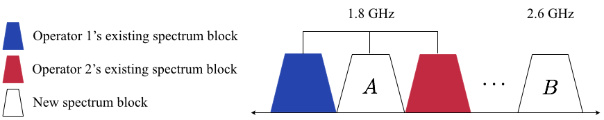
Figure 1: System model for spectrum auction.

II System Model and Game Formulation

II-A System Model

We consider two operators, say 1 and 2, bidding for two spectrum blocks $A$ and $B$ in a first-price sealed-bid auction as shown in Fig. 1. In this auction, the two operators simultaneously submit their bids in closed envelopes and the operator with the highest bid wins, and pays its bid for the spectrum block. Note that $A$ and $B$ are the same amount of downlink 10 MHz bandwidth. Without loss of generality, we consider only the downlink throughout the paper. Note that both operators deploy Frequency Division Duplex LTE (FDD LTE) and provide services to users in the same geography area.

Due to the operators’ existing spectrum holdings, the timing to launch the double-speed LTE services depends on the results of the LTE spectrum auction. If $A$ is assigned to operator 1, the double-speed LTE services are directly provided to users. On the other hand, the other operator 2 who acquires $B$ should deploy the inter-band non-contiguous CA to exploit fragmented spectrum, enabling to offer double-speed LTE service to users. However, it requires some deployment time $T$. For notational convenience, we assume that operator 1 acquires $A$, which will be relaxed in Section V.

Since the deployment time $T$ completely alters the nature of the operators’ dynamic pricing strategies and the user subscription dynamics, we analyze two phases $t<T$ and $t\geq T$, separately, by defining the following terms.

Definition 1.

(Asymmetric phase) Assume that operator 2 launches double-speed LTE service at time $T$. When $0\leq t<T$, we call this period asymmetric phase due to the different services provided operators 1 and 2.

Definition 2.

(Symmetric phase) When $t\geq T$, we call this period symmetric phase because of the same services offered by operators 1 and 2.

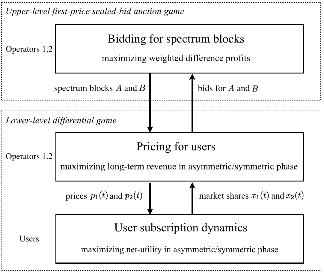
Figure 2: Hierarchical dynamic game framework for bidding, pricing, and user subscription dynamics.

II-B A Hierarchical Dynamic Game Framework

We formulate the interactions between the two operators and the users as a hierarchical dynamic game as shown in Fig. 2. The proposed game consists of two levels: an upper-level first-price sealed-bid auction game for bidding competition between two spiteful operators, and a lower-level differential game for dynamic pricing competition between them considering user subscription dynamics.

II-B1 Lower-level differential game

Users dynamically decide whether to stay in their current operator or to switch to the other operator for utility maximization. This user subscription dynamics depends on the perceived utilities, the operators’ current prices, switching costs, and price subsidies. Given the current operators’ market shares, the operators optimally set their service prices (i.e., time-dependent) to maximize their long-term revenues with the newly allocated spectrum. We model a differential game to completely characterize the operators’ dynamic pricing strategies and the corresponding user subscription dynamics in two phases.

II-B2 Upper-level first-price sealed-bid auction game

Two spiteful operators compete in a first-price sealed-bid auction based on the estimated revenues in the lower level. Since the realized profits are tightly coupled across the operators, the objective of each operator is maximizing the weighted difference of his own profit to that of his rival, where the weight $\gamma$ is the spite (or competition) coefficient that denotes the degree of competition.

III User Subscription Dynamics and Dynamic Pricing Competition in Asymmetric Phase

We consider a continuum of users that subscribes to one of the operators based on his or her operator preference. This continuum model, a widely used model to analyze the wireless communication industry, reflects the reality well if there are a sufficiently large number of users so that a single user is negligible [16, 17]. We assume that the total population is normalized to 1. Let $x_{i}(t)$ denote the market share of operator $i\in\{1,2\}$, where $x_{i}(0)=x_{i}^{0}\in[0,1]$ is the initial market share of operator $i$. We assume full market coverage, i.e., $x_{1}(t)+x_{2}(t)=1$. Such assumption approximates the real world in that global mobile-cellular penetration already stands at 96$\%$ [18]. We also assume that operators 1 and 2 provide same quality in communication services to the users so that they have the same reserve utility $u_{0}$ before spectrum allocation.

III-A Lower-level Differential Game in Asymmetric Phase

III-A1 User subscription dynamics model

In asymmetric phase, the users in operators 1 and 2 obtain different utilities, i.e.,

$$u_{1}(t)=(1+\eta)u_{0},\quad u_{2}(t)=u_{0},\quad 0\leq t\leq T,$$ (1)

where $\eta\in(0,1)$ is a user sensitivity parameter to the double-speed LTE service than existing one. It means that the users care more about the data rate as $\eta$ increases. The users in operator 2 have more incentive to switch to operator 1 as $\eta$ increases. When they decide to change operator 1, however, they face two different types of economic factors: switching cost and price subsidy. The former that a user has to pay when changing operators is the disutility that a user experiences, while the latter that the operators give a subsidy to attract their competitors’ users is the utility that a user receives. Different users confront with different levels of switching costs and price subsidies. To model such users’ heterogeneity, we assume that the price subsidy $p_{s}$ and the switching cost $c_{s}$ are variables over $[0,\underline{s}]$ and $[0,\overline{s}]$, respectively. For simplicity, we further assume that the net switching cost $s=c_{s}-p_{s}$, the difference between the switching cost and the price subsidy, is uniformly distributed in $[-\underline{s},\overline{s}]$ with $0<\underline{s}\leq\overline{s}$. When $s\rightarrow-\underline{s}$, the user has more incentive to switch to the other operator while the converse is when $s\rightarrow\overline{s}$.

Now let us focus on how user subscription dynamics works in asymmetric phase. In the following analysis, we restrict our attention to the case that the switching from one operator to another in both directions is always possible. Since the gain of one operator represents a loss to another operator under the full market coverage, this assumption implies that the two operators are competing fiercely for market share by retaining their own users as well as stealing their rival’s users. A user $k$ in operator $i\in\{1,2\}$, with net switching cost, $s_{k}$, observes the prices charged by operators 1 and 2 ($p_{1}(t)$ and $p_{2}(t)$). A user $k$ in operator $i$ will switch to operator $j\neq i$ if

$$u_{j}(t)-p_{j}(t)-s_{k}>u_{i}(t)-p_{i}(t).$$ (2)

Thus the mass of switching users from operator $i$ to $j$ is

$$q_{ij}(t)=\mathbb{P}[s_{k}<u_{j}(t)-u_{i}(t)-p_{j}(t)+p_{i}(t)].$$ (3)

Note that the mass of staying users in operator $i$ $q_{ii}(t)=1-q_{ij}(t)$.

Assuming that $p_{1}(t)-p_{2}(t)\in[\eta u_{0}-\underline{s},\eta u_{0}+\underline{s}]$ so that $q_{21}(t)$ and $q_{12}(t)$ belong to $(0,1)$, the net change in operator $i$’s market share in the infinitesimal time interval $(t,t+dt]$, the difference between the mass of switching users from operator $j$ to $i$ and the mass of switching users from operator $i$ to $j$, can be expressed as follows:

$$x_{i}(t+dt)-x_{i}(t)=q_{ji}(t)x_{j}(t)dt-q_{ij}x_{i}(t)dt.$$ (4)

Then each operator’s market share rate at time $t$ over $[0,T)$ is

$$\dot{x}_{1}(t) = \frac{\eta u_{0}-p_{1}(t)+p_{2}(t)+\underline{s}}{s_{1}}-\frac{2\underline{s}}{s_{1}}x_{1}(t),$$

$$\dot{x}_{2}(t) = -\frac{\eta u_{0}-p_{1}(t)+p_{2}(t)+\underline{s}}{s_{1}}+\frac{2\underline{s}}{s_{1}}(1-x_{2}(t)),$$ (5)

where $s_{1}=\underline{s}+\overline{s}$. Note that the rates $\dot{x}_{1}(t)$ and $\dot{x}_{2}(t)$ are functions of the current service prices $p_{1}(t)$ and $p_{2}(t)$, the current market shares $x_{1}(t)$ and $x_{2}(t)$, the user sensitivity parameter $\eta$, and the minimum (or maximum) of users’ net switching costs $\underline{s}$ (or $\overline{s}$).

III-A2 Operators’ pricing model

Given the user subscription dynamics (5), operators 1 and 2 simultaneously determine their prices $(p_{1}(t),p_{2}(t))$ so that their total revenues are maximized over $[0,T)$.

Similarly, each operator’s revenue rate at time $t$ in asymmetric phase can be written as follows:

$$r_{i}(t)=p_{i}(t)(x_{i}(t)+\dot{x}_{i}(t)),\;i\in\{1,2\}.$$ (6)

Here, the revenue rate is the sum of revenue from current users and revenue gain/loss from new/old users.

For each operator $i\in\{1,2\}$, the optimal pricing control problem over a finite-time horizon $[0,T)$ can be expressed as follows:

$$\bf{P1}\mathrel{\mathop{\mathchar 58\relax}}\;\;\; \max_{p_{i}(t)}\;\mathcal{R}_{i}^{AP}(p_{1}(t),p_{2}(t))=\int_{0}^{T}e^{-\rho t}r_{i}(t)dt,$$ (9)

$$\;\text{s.t.}\;\dot{x}_{1}(t)=\frac{\eta u_{0}-p_{1}(t)+p_{2}(t)+\underline{s}}{s_{1}}-\frac{2\underline{s}}{s_{1}}x_{1}(t),$$

$$\quad\;\;x_{1}(0)=x_{1}^{0},$$

where $\rho$ is the discount rate taking into account the time value of money, and $x_{1}^{0}$ is the initial market share of operator $1$. Since $\dot{x}_{2}(t)=-\dot{x}_{1}(t)$ and $x_{2}(0)=1-x_{1}(0)$ given the assumption of full market coverage, we can describe the user subscription dynamics constraints by only (8) and (9). Note that each operator’s pricing strategy depends on not only the competitor’s pricing strategy but also, the market share state (i.e., the market shares of the two operators) that evolves according to a user subscription dynamic constraint in (8). This allows us to formulate and analyze the optimization problem $\bf{P1}$ within the differential fame framework [20].

III-A3 Formulation of Differential Game

Now we formulate the dynamic pricing competition between the two operators as a finite-horizon differential game as follows.

• Players: two operators 1 and 2.

• Strategy space: operator 1 can choose price $p_{1}(t)$ from the continuous and bounded set $\mathcal{P}_{1}=[0,(1+\eta)u_{0}]$ while operator 2 can choose price $p_{2}(t)$ from $\mathcal{P}_{2}=[0,u_{0}]$. This is due to the assumption $x_{1}(t)+x_{2}(t)=1$ so that all users are served.

• Market share state: the market shares of the two operators constitute the market share state denoted by a vector $\mathbb{x}(t)=[x_{1}(t),x_{2}(t)]^{T}$, where the state is controlled by the user subscription dynamics constraint in (8).

• Payoff function: two operators want to maximize their total discounted revenues over a prespecified time horizon in (7), respectively.

III-B Closed-loop Nash Equilibrium in Asymmetric Phase

For the formulated finite-horizon differential game, we will investigate the two operators’ dynamic pricing competition and the corresponding user subscription dynamics. To understand the two operator’s dynamic pricing strategies in the differential games literature, we first want to point out two main types of strategies: open-loop strategies and closed-loop strategies. The open-loop strategies do not involve strategic interaction between the two operators through the evolution of the market share state over time and the corresponding adjustment in their prices. This means that the two operators announce their pricing strategies at the initial time and commit to them, regardless of how the market share state $\mathbb{x}(t)$ evolves. In this regard, the open-loop strategies are neither time-consistent nor subgame-perfect in general. On the other hand, the closed-loop strategies take into account the initial and current market share state, allowing the two operators to determine and adjust their pricing strategies as $\mathbb{x}(t)$ changes. Thus, we consider the closed-loop strategies to capture the price dynamics and the corresponding user subscription dynamics.

With the notion of closed-loop strategies, the (subgame-perfect) closed-loop Nash equilibrium is defined as follows: Definition 3 (Closed-loop Nash equilibrium). A pair of closed-loop strategies $(p_{1}^{\ast},p_{2}^{\ast})\in\mathcal{P}_{1}\times\mathcal{P}_{2}$ is called a closed-loop Nash equilibrium if the following holds:

$$\small\mathcal{R}_{i}^{AP}(p_{i}^{\ast}(\cdot),p_{j}^{\ast}(\cdot))\geq\mathcal{R}_{i}^{AP}(p_{i}(\cdot),p_{j}^{\ast}(\cdot)),$$

for all $p_{i}\in\mathcal{P}_{i}$, and for any initial market share $x_{i}(0)=x_{i}^{0}\in[0,1]$, $i=1,2,i\neq j$. At a closed-loop Nash equilibrium, no operator can increase its revenue by changing its strategy unilaterally, given the current pricing strategy of the other operator.

To obtain the closed-loop Nash equilibrium and the resultant user subscription dynamics, we need to first examine the necessary conditions by applying the Pontryagin maximum principle [21]. To this end, we introduce the Hamiltonian function for operator $i$ defined as:

$$\mathcal{H}_{i}(t)=r_{i}(t)+\lambda_{i}(t)\dot{x}_{1}(t),\quad\ i=\{1,2\},$$ (10)

where $\lambda_{i}(t)$ is the co-state variable of operator $i$ associated with the market share $x_{1}(t)$. For simplicity, we will drop the time dependence expression $t$ from all variables, unless specified otherwise.

Since the Hamiltonian function for operator $i$ is strictly concave in the price $p_{i}$, the necessary conditions for the closed-loop Nash equilibrium provide sufficient conditions for optimality, i.e.,

$$\dot{x}_{1} = \frac{\eta u_{0}-p_{1}+p_{2}+\underline{s}}{s_{1}}-\frac{2\underline{s}}{s_{1}}x_{1},\;\;\;\;x_{1}(0)=x_{1}^{0},$$ (11)

$$\frac{\partial\mathcal{H}_{i}}{\partial p_{i}} = 0,$$ (12)

$$\frac{\partial\lambda_{i}}{\partial t} = \rho\lambda_{i}-\frac{\partial\mathcal{H}_{i}}{\partial x_{1}}-\frac{\partial\mathcal{H}_{i}}{\partial p_{j}}\frac{\partial p_{j}}{\partial x_{1}},$$ (13)

$$\lambda_{i}(T) = 0.$$ (14)

Note that (12) is the maximum condition with respect to the strategy of operator $i$, (13) is the adjoint equation to describe the dynamics of the co-state variable, and (14) is the boundary condition for the terminal time of the co-state variable. We further note that the term $\frac{\partial\mathcal{H}_{i}}{\partial p_{j}}\frac{\partial p_{j}}{\partial x_{1}}$ in (13) affects how the two operators adjust their prices as $\mathbb{x}(t)$ evolves over time. By solving the above conditions, we can obtain the following proposition.

Proposition 1. Let

$$\small p_{1}^{\ast}(t,x_{1}^{\ast}(t))=\frac{\eta u_{0}+\overline{s}+2\underline{s}-e_{1}(t)-z(t)}{3}+\frac{s_{2}-k(t)}{3}x_{1}^{\ast}(t),$$ (15)

$$p_{2}^{\ast}(t,x_{1}^{\ast}(t))=\frac{-\eta u_{0}+2\overline{s}+\underline{s}+e_{2}(t)-z(t)}{3}-\frac{s_{2}-k(t)}{3}x_{1}^{\ast}(t),$$ (16)

$$x_{1}^{\ast}(t)=e^{\int_{0}^{t}\delta(\xi)d\xi}\left(x_{1}^{0}+\int_{0}^{t}e^{-\int_{0}^{\tau}\delta(\xi)d\xi}\zeta(\tau)d\tau\right),x_{2}^{\ast}(t)=1-x_{1}^{\ast}(t),$$ (17)

where

$$\lambda_{1}(t)=k(t)x_{1}^{\ast}(t)+e_{1}(t),\quad\lambda_{2}(t)=k(t)x_{2}^{\ast}(t)+e_{2}(t)$$

$$k(t)=\frac{\alpha_{1}\left(1-e^{\frac{2(\alpha_{1}-\alpha_{2})}{3s_{1}}(T-t)}\right)}{1-\frac{\alpha_{1}}{\alpha_{2}}e^{\frac{2(\alpha_{1}-\alpha_{2})}{3s_{1}}(T-t)}},\mu(t)=\frac{13\underline{s}+5\overline{s}+6k(t)}{9s_{1}}+\rho,$$

$$z(t)=\frac{2s_{2}}{3(1+\rho)}\left(1-e^{(1+\rho)(t-T)}\right),\zeta(t)=\frac{\eta u_{0}+2a+b+e_{1}(t)+e_{2}(t)}{3s_{1}},$$

$$e_{1}(t)=-e^{\int_{0}^{t}\mu(\xi)d\xi}\left(\int_{t}^{T}e^{-\int_{0}^{\tau}\mu(\xi)d\xi}\nu(\tau)d\tau\right),e_{2}(t)=e_{1}(t)-z(t),$$

$$\delta(t)=\frac{2(k(t)-b-2a)}{3s_{1}},\nu(t)=\frac{\left(2s_{2}+3k(t)\right)\left(z(t)-2\underline{s}-\overline{s}-\eta u_{0}\right)}{9s_{1}},$$

and $\alpha_{1}$ and $\alpha_{2}$ are the solutions of the quadratic equation $\frac{2}{3s_{1}}k(t)^{2}-\left(\frac{11\overline{s}+25\underline{s}+9s_{1}\rho)}{9s_{1}}\right)k(t)+\frac{2}{9}s_{2}=0$. Then, ($p_{1}^{\ast},p_{2}^{\ast})$ constitute a closed-loop Nash equilibrium and $(x_{1}^{\ast},x_{2}^{\ast})$ are the corresponding user subscription dynamics of the problem $\bf{P1}$. Proof. See Appendix A. $\blacksquare$

IV User Subscription Dynamics and Dynamic Pricing Competition in Symmetric Phase

In the previous section, we have studied the dynamic pricing competition of the two operators and the corresponding user subscription dynamics in asymmetric phase. In this section, we consider them in symmetric phase by formulating an infinite-horizon differential game. The analysis is similar to the previous section and thus this section is brief.

IV-A Lower-level Differential Game in Symmetric Phase

IV-A1 User subscription dynamics model

Since operator $2$ launches double-speed LTE service in symmetric phase, we assume that the users in operators $1$ and $2$ obtain same utility, i.e.,

$$u_{1}(t)=u_{2}(t)=(1+\eta)u_{0},\quad t>T.$$ (18)

Similar to the analysis in Sec. III-A, assuming that $p_{1}(t)-p_{2}(t)\in[-a,a]$ so that $q_{21}(t)$ and $q_{12}(t)$ belong to $(0,1)$, each operator’s market share rate at time $t$ over $[T,\infty)$ is

$$\dot{x}_{1}(t)=\frac{p_{2}(t)-p_{1}(t)+\underline{s}}{s_{1}}-\frac{2\underline{s}}{s_{1}}x_{1}(t)=-\dot{x}_{2}(t).$$ (19)

IV-A2 Operators’ pricing model

Given the user subscription dynamics (19), each operator’s revenue rate at time $t$ in symmetric phase can be written as follows:

$$r_{i}(t)=p_{i}(t)(x_{i}(t)+\dot{x}_{i}(t)),\;i\in\{1,2\}.$$ (20)

For each operator $i\in\{1,2\}$, the optimal pricing control problem over an infinite-time horizon $[T,\infty)$ can be expressed as follows.

$$\bf{P2}\mathrel{\mathop{\mathchar 58\relax}}\;\;\; \max_{p_{i}(t)}\;\mathcal{R}_{i}^{SP}(p_{1}(t),p_{2}(t))=\int_{T}^{\infty}e^{-\rho t}r_{i}(t)dt,$$ (23)

$$\;\text{s.t.}\;\dot{x}_{1}(t)=\frac{p_{2}(t)-p_{1}(t)+\underline{s}}{s_{1}}-\frac{2\underline{s}}{s_{1}}x_{1}(t),$$

$$\quad\;\;\;\;\;x_{1}(T)=x_{1}^{T},$$

where $x_{1}^{T}$ is the initial market share of operator $1$ from the end of asymmetric phase.

IV-A3 Formulation of differential game

The dynamic pricing competition between the two operators can be formulated as an infinite-horizon differential game as follows.

• Players: two operators 1 and 2.

• Strategy space: operator $i$ can choose price $p_{i}(t)$ from the continuous and bounded set $\mathcal{P}_{i}=[0,(1+\eta)u_{0}]$ for $i=1,2$.

• Market share state: the market share state $\mathbb{x}(t)=[x_{1}(t),x_{2}(t)]^{T}$ is controlled by the user subscription dynamics constraint in (19).

• Payoff function: the two operators want to maximize their total discounted revenues over a prespecified time horizon in (21), respectively.

IV-B Closed-loop Nash Equilibrium in Symmetric Phase

To proceed with the analytical solution of the formulated infinite-horizon differential game, we now focus on the closed-loop Nash equilibrium solutions and the consequent user subscription dynamics of the problem $\bf{P2}$. Recall that at a closed-loop Nash equilibrium, no operator has an incentive to deviate from its strategy after considering the other operator’s strategy. The closed-loop Nash equilibrium and the consequent user subscription dynamics are given in the following proposition.

Proposition 2. Let

$$\small p_{1}^{\ast}(t,x_{1}^{\ast}(t))=\frac{s_{1}+\underline{s}+e_{2}-2e_{1}}{3}+\frac{s_{2}-k}{3}x_{1}^{\ast}(t),$$ (24)

$$\small p_{2}^{\ast}(t,x_{1}^{\ast}(t))=\frac{s_{1}+\overline{s}+2e_{2}-e_{1}}{3}-\frac{s_{2}-k}{3}x_{1}^{\ast}(t),$$ (25)

$$\small x_{1}^{\ast}(t)=\frac{1}{2}+\left(x_{1}^{T}-\frac{1}{2}\right)e^{\frac{2(k-\underline{s}-s_{1})}{3s_{1}}(t-T)},\quad x_{2}^{\ast}(t)=1-x_{1}^{\ast}(t),$$ (26)

where $k$ is the smallest root of the quadratic equation

$$\small 6k^{2}-\left(11\overline{s}+25\underline{s}+9\rho s_{1}\right)k+2s_{2}^{2}=0,$$

and

$$\small e_{1}=\frac{s_{2}}{3(1+\rho)}+\frac{s_{2}^{2}-3k(2\underline{s}+\overline{s})}{6k-13\underline{s}-5\overline{s}-9\rho s_{1}},e_{2}=e_{1}-\frac{2s_{2}}{3(1+\rho)}.$$

Then, $(p_{1}^{\ast},p_{2}^{\ast})$ constitute a closed-loop Nash equilibrium and $(x_{1}^{\ast},x_{2}^{\ast})$ are the corresponding user subscription dynamics of the problem $\bf{P2}$. Proof. See Appendix B. $\blacksquare$

V Bidding Competition

In the upper level, the two spiteful operators compete in a first-price sealed-bid auction where asymmetric-valued spectrum blocks $A$ and $B$ are auctioned off to them. For fair competition, each operator is constrained to lease only one spectrum block (i.e., $A$ or $B$). We assume that the regulators set the reserve prices $c^{A}$ and $c^{B}$ to $A$ and $B$, respectively. Note that reserve price is the minimum price to get the spectrum block. Since $A$ is the high-valued spectrum block, we further assume that the two spiteful operators are only competing on $A$ to provide double-speed LTE service to their users earlier.

Based on the projected total revenues of the two operators in the lower level, operators 1 and 2 bid $A$ independently as $b_{1}$ and $b_{2}$, respectively. In this case, $B$ is assigned to the operator who loses in the auction as the reserve price $c^{B}$. Since this operator should make huge investments to double the existing LTE network capacity compared to the other MNO, we also assume the only operator who acquires $B$ incurs the investment cost $c^{BS}$.

For notational convenience, we have assumed that operator 1 procures $A$ throughout the paper. Without loss of generality, however, we can relax this assumption easily after some algebraic manipulations. The projected aggregate revenues of the two operators over the entire time-horizon $[0,\infty]$ can be expressed as follows:

• Assuming that operators 1 and 2 acquire $A$ and $B$ respectively, each operator’s projected aggregate revenue during the entire period is

  $$\mathcal{R}_{1}^{A}=\mathcal{R}_{1}^{AP}+\mathcal{R}_{1}^{SP},\quad\mathcal{R}_{2}^{B}=\mathcal{R}_{2}^{AP}+\mathcal{R}_{2}^{SP},$$ (27)

  where $\mathcal{R}_{i}^{AP}$ and $\mathcal{R}_{i}^{SP}$ are described in (7) and (21), respectively, for $i=1,2$.

• Assuming that operators 1 and 2 procure $B$ and $A$ respectively, each operator’s projected aggregate revenue during the entire period is

  $$\mathcal{R}_{1}^{B}=\mathcal{R}_{1}^{AP^{{}^{\prime}}}+\mathcal{R}_{1}^{SP^{{}^{\prime}}},\quad\mathcal{R}_{2}^{A}=\mathcal{R}_{2}^{AP^{{}^{\prime}}}+\mathcal{R}_{2}^{SP^{{}^{\prime}}},$$ (28)

  where $\mathcal{R}_{i}^{AP^{{}^{\prime}}}$ and $\mathcal{R}_{i}^{SP^{{}^{\prime}}}$ for $i=1,2$ can be obtained by reformulating the problems $\bf{P1}$ and $\bf{P2}$, and following the same steps as in Appendices $A$ and $B$. Details are omitted for brevity.

When asymmetric-valued spectrum blocks are allocated to the operators, there is a trade-off between self-interest and spite. To illustrate this trade-off, we first restrict ourselves to the case where the spite is not present. If operator $i$ is self-interested, his objective function is as follows:

$$\Pi_{i}(b_{i},b_{j})=\left[\mathcal{R}_{i}^{A}-b_{i}\right]\cdot I_{b_{i}\geq b_{j}}+\pi_{i}^{B}\cdot I_{b_{i}\leq b_{j}},i=1,2,i\neq j,$$ (29)

where $I$ is the indicator function and $\pi_{i}^{B}=\mathcal{R}_{i}^{B}-c^{B}-c^{BS}$ is the profit from $B$ for $i=1,2$. This is the standard auction framework in that operator $i$ maximizes his own profit without considering the profit of his competitor.

In the real world, however, there are observations that some operators are completely malicious [13]. If operator $i$ is completely malicious, his objective function can be changed as follows:

$$\Pi_{i}(b_{i},b_{j})=-\pi_{j}^{B}\cdot I_{b_{i}\geq b_{j}}-\left[\mathcal{R}_{j}^{A}-b_{j}\right]\cdot I_{b_{i}\leq b_{j}},i=1,2,i\neq j,$$ (30)

It means that operator $i$ only intends to minimize the profit of operator $j$.

Departing from the standard auction framework, our model incorporates this strategic concern in that each spiteful operator cares about maximizing the weighted difference of his own profit to that of his competitor. Combining (29) and (30), we define each operator’s objective function as follows.

Definition 4. Assume that two spiteful operators (i.e., $i=1,2$ and $i\neq j$) compete in a first-price sealed-bid auction. The objective function that each operator tries to maximize is given by:

$$\Pi_{i}(b_{i},b_{j})= \left[(1-\gamma)(\mathcal{R}_{i}^{A}-b_{i})-\gamma\pi_{j}^{B}\right]\cdot I_{b_{i}\geq b_{j}}$$ (31)

$$+ \left[(1-\gamma)\pi_{i}^{B}-\gamma\left(\mathcal{R}_{j}^{A}-b_{j}\right)\right]\cdot I_{b_{i}\leq b_{j}},$$

where $I$ is the indicator function, $\pi_{i}^{B}=\mathcal{R}_{i}^{B}-c^{B}-c^{BS}$ is the profit from $B$, and $\gamma\in[0,1]$ is a parameter called the spite (or competition) coefficient.

Note that (31) will be used to determine the bidding strategies of two spiteful operators, which does not affect the realized profits of the two operators. As described, operator $i$ is self-interested and only intends to maximize his own profit when $\gamma=0$. When $\gamma=1$, operator $i$ is completely malicious and only tries to minimize the profit of his competitor. For given $\gamma\in[0,1]$, we can derive the optimal bidding strategies that maximize the objective function in Definition 4 as follows.

Proposition 3. In a first-price sealed-bid auction, the equilibrium bidding strategies for two operators 1 and 2 are given by

$$b^{\ast}_{1}(\gamma)=\frac{(1-\gamma)(\mathcal{R}_{1}^{A}+c^{A}-\pi_{1}^{B})+\gamma(\mathcal{R}_{2}^{A}-\pi_{2}^{B})}{2-\gamma},$$

$$b^{\ast}_{2}(\gamma)=\frac{(1-\gamma)(\mathcal{R}_{2}^{A}+c^{A}-\pi_{2}^{B})+\gamma(\mathcal{R}_{1}^{A}-\pi_{1}^{B})}{2-\gamma}.$$ (32)

Proof. See Appendix C. $\blacksquare$

VI Numerical Results

In this section, several numerical results are presented to investigate the impact of spectrum allocation on market structure, and provide insights into the role of the regulator. For illustration convenience, we assume that operators 1 and 2 acquire the spectrum blocks $A$ and $B$, respectively, unless otherwise specified.

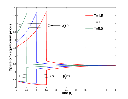
(a) Dynamic pricing strategies of operator 1 and operator 2

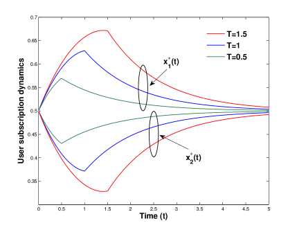
(b) User subscription dynamics

Figure 3: The dynamics of user subscription and the two operators’ pricing strategies. Other parameters are $u_{0}=10$, $\eta=0.5$, $\rho=0.5$, $\underline{s}=5$, and $\overline{s}=10$.

VI-A Dynamics of Pricing Competition and User Subscription

We first study the impact of spectrum allocation on the two operators’ dynamic pricing strategies and the the resultant user subscription dynamics. As a benchmark, we focus on the symmetric market share before spectrum allocation where the initial market state of the two operators are chosen as $\mathbb{x}(0)=[0.5,0.5]$.

Fig. 3 shows the two operators’ equilibrium pricing strategies and the corresponding user subscription dynamics under different deployment times. In asymmetric phase $(t<T)$, due to the earlier launch of double-speed LTE service, we see that operator 1 becomes the market share leader while charging a higher price. An interesting observation is that $p_{1}^{\ast}(t)$ and $x_{1}^{\ast}(t)$ increase in $t$, while the reverse is true for operator 2. These phenomena are due to the presence of the users’ net switching costs. As $t$ increases, the more users with the high net switching costs are locked in, allowing operator 1 to optimally raise $p_{1}^{\ast}(t)$ by the amount of the net switching costs with the increase in $x_{1}^{\ast}(t)$. This forces operator 2 to reduce $p_{2}^{\ast}(t)$ but with the decrease in $x_{2}^{\ast}(t)$. The users’ net switching costs, thus, can be interpreted as a subsidy for operator 1 and a tax for operator 2. It is also worth pointing out that the longer deployment time $T$ is the slower rate of increase of $p_{1}^{\ast}(t)$ for operator 1, while the faster rate of decrease of $p_{2}^{\ast}(t)$ for operator 2 at the lower initial prices $p_{1}^{\ast}(0)$ and $p_{2}^{\ast}(0)$. With the longer $T$, operator 1 has more to gain by charging $p_{1}^{\ast}(t)$ less aggressively and attaining $x_{1}^{\ast}(t)$ more aggressively for the same $t$, thereby maximizing the aggregated revenue $\mathcal{R}_{1}^{AP}(T)$ over $[0,T)$. On the other hand, operator 2 tries to maximize $\mathcal{R}_{2}^{AP}(T)$ by decreasing $p_{2}^{\ast}(t)$ more aggressively, but losing more $x_{2}^{\ast}(t)$ for the same $t$.

In symmetric phase ($t\geq T$), due to the same services offered by the two operators 1 and 2, each operator faces a trade-off between a low price to increase its market share, and a high price to harvest its revenue by exploiting users’ net switching costs. As shown in Fig. 3, the large operator 1 charges a high price while the small operator 2 charges a low price. Thus, the asymmetries of their market shares and prices fade away over time, resulting in symmetric outcomes in steady state. We also observe that the slower rate of the steady state as $T$ increases.

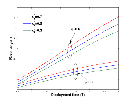
Figure 4: Revenue gain as a function of $T$ under different parameters $\mathbb{x}(0)$ and $\eta$. Other parameters are $u_{0}=10$, $\rho=0.5$, $\underline{s}=5$, and $\overline{s}=10$.

VI-B Values of Contiguous and Non-contiguous Spectrum

In this subsection, we examine the values of two different spectrum blocks: contiguous spectrum block $A$ and non-contiguous spectrum block $B$. To this end, we define the revenue gain as follows:

$$\mathcal{R}_{gain}=\frac{\mathcal{R}_{i}^{A}}{\mathcal{R}_{j}^{B}},\quad i=1,2,\quad i\neq j.$$ (33)

Fig. 4 shows how $\mathcal{R}_{gain}$ changes in $T$ with different parameters $\eta$ and $\mathbb{x}(0)$. Intuitively, the revenue gain is strictly increasing over $T$ and this gain becomes much higher as $\eta$ or $x_{1}^{0}$ increase. It explains how critical new spectrum is allocated to both operators, and why they should spitefully bid in a first-price sealed-bid auction to achieve a dominant position or compensate the revenue gap. It also indicates that the asymmetric-valued LTE spectrum allocation should be carefully tailored to avoid excessive competition, and promote fair competition between operators.

VI-C Bidding Strategies and Resultant Profits

Based on the estimated values of two different spectrum blocks, we investigate the two operators’ equilibrium bidding strategies and their corresponding profits. To this end, the initial market share state are set to $\mathbb{x}(0)=[0.6,0.4]$. Fig. 5 shows how the two operator’s equilibrium bidding strategies realize when the spite coefficient $\gamma$ varies under two different deployment times. Intuitively, the more spiteful the two operators are, the more aggressively they tend to bid. Since more spiteful operator gets more disutility from the profit of his competitor, he is willing to sacrifice some monetary payoff in order to minimize his rival’s profit. It is worth noting that there is a cross-over point at $\gamma=0.5$. This can be interpreted as the different levels of the utility (or disutility) of winning (or losing) the auction between the two operators. When $\gamma<0.5$, the more emphasis they put on their own profits, inducing operator 1 to place a higher bid because he could make more profit from $A$. When $\gamma>0.5$, on the other hand, they are more interested in minimizing the profits of their competitors, prompting operator 2 to bid more aggressively since she could reduce operator 1’s profit more when acquiring $A$, and thus increase her relative position in the market. This may explains why Korea Telecom (i.e., a small operator) placed a bid twice as high as SK Telecom (i.e., a large operator) for procuring the contiguous spectrum block [6]. We also observe that the equilibrium bidding strategies of the two operator increase as $T$ increases. It implies that the longer $T$ promotes the more fierce competition between operators.

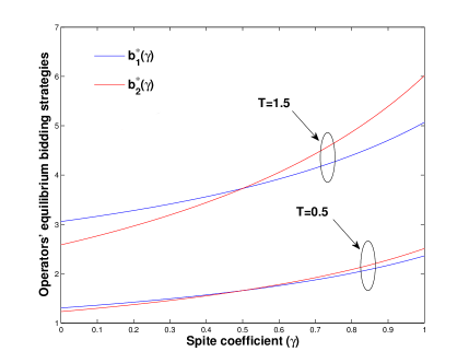
Figure 5: The equilibrium bidding strategies of two operators as a function of $\gamma$ under two different deployment times. Other parameters are $u_{0}=10$, $\eta=0.5$, $\rho=0.5$, $\underline{s}=5$, $\overline{s}=10$, $c^{A}=0.1$, $c^{B}=0.2$, and $c^{BS}=1$.

Fig. 6 shows the resultant profits of the two operators as a function of $\gamma$ under two different deployment times. When $\gamma<0.5$, the two operators are more interested in maximizing their profits, resulting in the large difference between their profits as $T$ increases or $\gamma$ decreases. It implies that the small operator 2 should place a more spiteful bid as $T$ increases in order to improve (or maintain) his own standing in a highly competitive market. When $\gamma>0.5$, the difference between their profits decreases as $T$ decreases for the same $\gamma$, allowing operator 2 to increase his relative position in the market by bidding more aggressively. However, when $\gamma=0.6$ and $T=1.5$, the profit of operator 2 is is more than 35% compared with that of operator 1. It offers meaningful insights into the role of the regulators in that the longer $T$ hinders fair competition between the two operators. Thus, the regulators should appropriately impose limits on the timing of the double-speed LTE services. In South Korea, for example, Korea Telecom (KT) who secured the contiguous spectrum could not start its double-speed LTE services in major cities until March 2014, and nation-wide coverage until July [6]. This gave its competitors time to roll out the LTE-Advanced services, allowing to promote fair competition between operators.

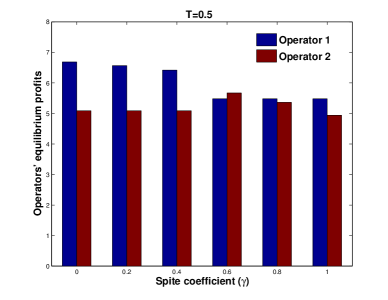
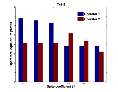
Figure 6: The equilibrium profits of two operators as a function of $\gamma$ under two different deployment times. $u_{0}=10$, $\eta=0.5$, $\rho=0.5$, $\underline{s}=5$, $\overline{s}=10$, $c^{A}=0.1$, $c^{B}=0.2$, and $c^{BS}=1$.

VII Conclusion

This paper presents a comprehensive analytical and numerical studies of the effects of asymmetric-valued LTE spectrum allocation. We model the interactions between operators and users as a hierarchical dynamic game framework, where two spiteful operators simultaneously make spectrum acquisition decisions in the upper-level first-price seals-bid auction game, and dynamic pricing decisions in the lower-level differential game, taking into account user subscription dynamics. Using backward induction, we derive and characterize the equilibrium of the entire game under mild conditions. Through analytical and numerical results, we verify our studies by comparing the latest results of LTE spectrum auction in South Korea. This serves as the benchmark of asymmetric-valued LTE spectrum allocation.

The weakness of this study is the same spite between two operators. Depending on the relative position in the market, operators may take the profits of them into account differently. This broader setting where operators are asymmetric spiteful makes our studies more applicable for extensive spectrum allocation scenarios and gives more insights into the role of regulation.

VIII Appendix

VIII-A Proof of Proposition 1

From (12), we have the two operators’ best response functions,

$$\small p_{1}=\frac{1}{2}\left(p_{2}+\eta u_{0}+\underline{s}-\lambda_{1}+sx_{1}\right),p_{2}=\frac{1}{2}\left(p_{1}-\eta u_{0}+\overline{s}+\lambda_{2}-s_{2}x_{1}\right].$$ (34)

Using them gives equilibrium prices,

$$\small p_{1}=\frac{1}{3}\left(\eta u_{0}+s_{1}+\underline{s}-2\lambda_{1}+\lambda_{2}+s_{2}x_{1}\right),$$

$$\small p_{2}=\frac{1}{3}\left(-\eta u_{0}+s_{1}+\overline{s}-\lambda_{1}+2\lambda_{2}-s_{2}x_{1}\right).$$ (35)

Next, from (13) and (35), we obtain the following partial differential equations,

$$\small\dot{\lambda}_{1}=\rho\lambda_{1}-\frac{2p_{1}s_{2}-\lambda_{1}(5\underline{s}+\overline{s})}{3s_{1}},\dot{\lambda}_{2}=\rho\lambda_{2}-\frac{-2p_{2}s_{2}-\lambda_{2}(5\underline{s}+\overline{s})}{3s_{1}}.$$ (36)

We solve this system of differential equations by the method of undetermined coefficients. Assume that $\lambda_{i}(t)=k_{i}(t)x_{1}(t)+e_{i}(t)$ for $i=1,2$. Substitution into (36) yields

$$\small\dot{k}_{1}x_{1}+k_{1}\dot{x}_{1}+\dot{e}_{1}=\rho\left(k_{1}x_{1}+e_{1}\right)-\frac{2p_{1}s_{2}-(k_{1}x_{1}+e_{1})(5\underline{s}+\overline{s})}{3s_{1}},$$ (37)

$$\small\dot{k}_{2}x_{1}+k_{2}\dot{x}_{1}+\dot{e}_{2}=\rho\left(k_{2}x_{1}+e_{2}\right)-\frac{-2p_{2}s_{2}-(k_{2}x_{1}+e_{2})(5\underline{s}+\overline{s})}{3s_{1}},$$ (38)

where $\dot{x}_{1}$ is given in (8). Since the equalities in (37) and (38) must hold for all values of $x_{1}$, the coefficients of $x_{1}$ and the constant terms have to be zero. Define $y(t)=k_{1}(t)-k_{2}(t)$ and $z(t)=e_{1}(t)-e_{2}(t)$. Subtracting (38) from (37) yields

$$\small\dot{y}-\left(\frac{k_{1}+k_{2}+7\underline{s}+5\overline{s}+3\rho s_{1}}{3s_{1}}\right)y=0,\quad\dot{z}-(1+\rho)z+\frac{2s_{2}}{3}=0.$$ (39)

Using the integrating factor method under the boundary conditions $\lambda_{i}(T)=0$ for $i=1,2$, which implies $k_{i}(T)=e_{i}(T)=0$ for $i=1,2$, we obtain

$$\small y(t)=0,\quad z(t)=\frac{2s_{2}}{3(1+\rho)}\left(1-e^{(1+\rho)(t-T)}\right),$$ (40)

which follows that $k_{1}(t)=k_{2}(t)$ and $e_{1}(t)=e_{2}(t)+z(t)$.

With the above results, setting $k(t)=k_{1}(t)=k_{2}(t)$ and rewriting (37) and (38) give

$$\small\dot{k}=-\frac{2}{3s_{1}}k^{2}+\left(\frac{11\overline{s}+25\underline{s}+9\rho s_{1})}{9s_{1}}\right)k-\frac{2}{9}s_{2},\\$$ (41)

$$\small\dot{e}_{1}=\left(\frac{13\underline{s}+5\overline{s}+6k}{9s_{1}}+\rho\right)e_{1}-\frac{(2s_{2}+3k)(s_{1}+\underline{s}+\eta u_{0}-z)}{9s_{1}}.$$ (42)

First, consider the Riccati differential equation (41). Let $\alpha_{1}$ and $\alpha_{2}$ are the two solutions of the quadratic equation, i.e.,

$$\small\frac{2}{3s_{1}}k^{2}-\left(\frac{11\overline{s}+25\underline{s}+9\rho s_{1}}{9s_{1}}\right)k+\frac{2}{9}s_{2}=0.$$ (43)

Without loss of generality, assume $\alpha_{1}<\alpha_{2}$. Note that the two solutions $\alpha_{1}$ and $\alpha_{2}$ are particular solutions of (41). Then a general solution of (41) is (see [21])

$$\small\frac{k(t)-\alpha_{1}}{k(t)-\alpha_{2}}=Ce^{-\frac{2(\alpha_{1}-\alpha_{2})}{3s_{1}}t},$$ (44)

where $C$ is the constant of integration. Using the boundary condition $k(T)=0$, the constant $C$ is $\frac{\alpha_{1}}{\alpha_{2}}e^{\frac{2(\alpha_{1}-\alpha_{2})}{3s_{1}}T}$, which yields

$$\small k(t)=\frac{\alpha_{1}\left(1-e^{\frac{2(\alpha_{1}-\alpha_{2})}{3s_{1}}(T-t)}\right)}{1-\frac{\alpha_{1}}{\alpha_{2}}e^{\frac{2(\alpha_{1}-\alpha_{2})}{3s_{1}}(T-t)}}.$$ (45)

Next, consider the first order partial differential equation (42). Let $\mu(t)=\frac{13\underline{s}+5\overline{s}+6k(t)}{9s_{1}}+\rho$ and $\nu(t)=\frac{\left(2s_{2}+3k(t)\right)\left(z(t)-2\underline{s}-\overline{s}-\eta u_{0}\right)}{9s_{1}}$. Using the integrating factor method under the boundary conditions $e_{i}(T)=0$ for $i=1,2$, we have

$$\small e_{1}(t)=-e^{\int_{0}^{t}\mu(\xi)d\xi}\left(\int_{t}^{T}e^{-\int_{0}^{\tau}\mu(\xi)d\xi}\nu(\tau)d\tau\right),e_{2}(t)=e_{1}(t)-z(t),$$ (46)

Then the equilibrium prices can be rewritten as

$$\small p_{1}^{\ast}(t,x_{1}(t))=\frac{\eta u_{0}+\overline{s}+2\underline{s}-e_{1}(t)-z(t)}{3}+\frac{s_{2}-k(t)}{3}x_{1}(t),$$ (47)

$$\small p_{2}^{\ast}(t,x_{1}(t))=\frac{-\eta u_{0}+2\overline{s}+\underline{s}+e_{2}(t)-z(t)}{3}-\frac{s_{2}-k(t)}{3}x_{1}(t).$$ (48)

Now, operator 1’s market share rate in (8) can be expressed as

$$\small\dot{x}_{1}=\frac{\eta u_{0}+2\underline{s}+\overline{s}+e_{1}+e_{2}}{3s_{1}}+\frac{2(k-\overline{s}-2\underline{s})}{3s_{1}}x_{1},$$ (49)

where his initial market share is $x_{1}^{0}$. Using the integrating factor method yield

$$\small x_{1}^{\ast}(t)=e^{\int_{0}^{t}\delta(\xi)d\xi}\left(x_{1}^{0}+\int_{0}^{t}e^{-\int_{0}^{\tau}\delta(\xi)d\xi}\zeta(\tau)d\tau\right),$$ (50)

where $\delta(t)=\frac{2(k(t)-b-2a)}{3(a+b)}$ and $\zeta(t)=\frac{\eta u_{0}+2a+b+e_{1}(t)+e_{2}(t)}{3(a+b)}$, which completes the proof.

VIII-B Proof of Proposition 2

We proceed by following the similar steps as in Appendix A. The Hamiltonian function for operator $i$ is

$$\mathcal{H}_{i}=\left(r_{i}(t)+\lambda_{i}(t)\dot{x}_{1}(t)\right),\quad\ i=\{1,2\},$$ (51)

Due to the concavity of Hamiltonian function with respect to $p_{i}$, the necessary conditions for the feedback Nash equilibrium provide sufficient conditions for optimality, i.e.,

$$\dot{x}_{1} = \frac{p_{2}-p_{1}+\underline{s}}{s_{1}}-\frac{2\underline{s}}{s_{1}}x_{1},\quad x_{1}(T)=x_{1}^{T},$$ (52)

$$\frac{\partial\mathcal{H}_{i}}{\partial p_{i}} = 0,$$ (53)

$$\frac{\partial\lambda_{i}}{\partial t} = \rho\lambda_{i}-\frac{\partial\mathcal{H}_{i}}{\partial x_{1}}-\frac{\partial\mathcal{H}_{i}}{\partial p_{j}}\frac{\partial p_{j}}{\partial x_{1}},$$ (54)

$$\lim_{t\to\infty}e^{-\rho t}\lambda_{i}(t) = 0.$$ (55)

Note that the terminal condition in (55) is different from (14).

From (53), the equilibrium prices are

$$\small p_{1}=\frac{1}{3}\left(s_{1}+\underline{s}-2\lambda_{1}+\lambda_{2}+s_{2}x_{1}\right),p_{2}=\frac{1}{3}\left(s_{1}+\overline{s}-\lambda_{1}+2\lambda_{2}-s_{2}x_{1}\right).$$ (56)

From (54) and (56), we have

$$\small\dot{\lambda}_{1}=\rho\lambda_{1}-\frac{2p_{1}s_{2}-\lambda_{1}(5\underline{s}+\overline{s})}{3s_{1}},\dot{\lambda}_{2}=\rho\lambda_{2}-\frac{-2p_{2}s_{2}-\lambda_{2}(5\underline{s}+\overline{s})}{3s_{1}}.$$ (57)

We solve this system of differential equations by the method of undetermined coefficients. Assume that $\lambda_{i}(t)=k_{i}x_{1}(t)+e_{i}$ for $i=1,2$. Note that the coefficients of $x_{1}(t)$ and the constant terms are not functions of time when the time horizon is infinite. Substitution into (47) yields

$$\small k_{1}\dot{x}_{1}=\rho(k_{1}x_{1}+e_{1})-\frac{2p_{1}s_{2}-(k_{1}x_{1}+e_{1})(5\underline{s}+\overline{s})}{3s_{1}},$$ (58)

$$\small k_{2}\dot{x}_{1}=\rho(k_{2}x_{1}+e_{2})+\frac{2p_{1}s_{2}+(k_{2}x_{1}+e_{2})(5\underline{s}+\overline{s})}{3s_{1}}.$$ (59)

Subtracting (59) from (58), as in the proof of Proposition 1, we can show that

$$\small k_{1}=k_{2}=\frac{11\overline{s}+25\underline{s}+9\rho s_{1}-\sqrt{\left(11\overline{s}+25\underline{s}+9\rho s_{1}\right)^{2}-48(s_{2})^{2}}}{12},$$

$$\small e_{1}=e_{2}+\frac{2s_{2}}{3(1+\rho)}.$$ (60)

where $k_{1}$ (or $k_{2}$) is the smallest root of the quadratic equation

$$\small 6k^{2}-\left(11\overline{s}+25\underline{s}+9\rho s_{1}\right)k+2s_{2}^{2}=0.$$

Let $k=k_{1}=k_{2}$. Using (58), (59), and (60) we have

$$\small e_{1}=\frac{s_{2}}{3(1+\rho)}+\frac{s_{2}^{2}-3k(2\underline{s}+\overline{s})}{6k-13\underline{s}-5\overline{s}-9\rho s_{1}},k=-e_{1}-e_{2}.$$ (61)

Then, the equilibrium prices can be rewritten as

$$\small p_{1}^{\ast}(t,x_{1}(t))=\frac{s_{1}+\underline{s}+e_{2}-2e_{1}}{3}+\frac{s_{2}-k}{3}x_{1}(t),$$ (62)

$$\small p_{2}^{\ast}(t,x_{1}(t))=\frac{s_{1}+\overline{s}+2e_{2}-e_{1}}{3}-\frac{s_{2}-k}{3}x_{1}(t).$$ (63)

Following similar steps in (49) and (50), user subscription dynamics in symmetric phase can be written as

$$\small x_{1}^{\ast}(t)=\frac{1}{2}+\left(x_{1}^{T}-\frac{1}{2}\right)e^{\frac{2(k-\underline{s}-s_{1})}{3s_{1}}(t-T)},\quad x_{2}^{\ast}(t)=1-x_{1}^{\ast}(t),$$ (64)

which completes the proof.

VIII-C Proof of Proposition 3

Without loss of generality, suppose that operator $i$ knows his bid $b_{i}$. Further, we assume that operator $i$ infer that the bidding strategy of operator $j$ on $A$ is drawn uniformly and independently from $[c^{A},\mathcal{R}_{j}^{A}]$. The operator $i$’s optimization problem is to choose $b_{i}$ to maximize the expectation of

$$\mathrm{E}_{b_{i}}(\Pi_{i})= \int_{c^{A}}^{b_{i}}\left[(1-\gamma)(\mathcal{R}_{i}^{A}-b_{i})-\gamma\pi_{j}^{B}\right]f(b_{j})db_{j}$$ (65)

$$+ \int_{b_{i}}^{\mathcal{R}_{j}^{A}}\left[(1-\gamma)\pi_{i}^{B}-\gamma\left(\mathcal{R}_{j}^{A}-b_{j}\right)\right]f(b_{j})db_{j}.$$

Differentiating (65) with respect to $b_{i}$, setting the result to zero and multiplying by $\mathcal{R}_{j}^{A}-c^{A}$ give

$$\frac{\partial\mathrm{E}_{b_{i}}(\Pi_{i})}{\partial b_{i}}=(1-\gamma)\left(\mathcal{R}_{i}^{A}+c^{A}-\pi_{i}^{B}\right)+\gamma\left(\mathcal{R}_{j}^{A}-\pi_{j}^{B}\right)-(2-\gamma)b_{i}=0.$$

Applying the same way to operator $j$ completes the proof.

References

- [1] Cisco, “Cisco visual networking index: global mobile data traffic forecast update, 2014-2019,” White paper, Feb. 2015.
- [2] 4G Americas, “Meeting the 1000x challenge: The need for spectrum, technology and policy innovations,” White paper, Oct. 2013.
- [3] J. Huang and L. Gao, Wireless Network Pricing, Synthesis Lectures on Communication Networks, Morgan & Claypool, 2013.
- [4] M. J. Marcus, “Spectrum policy and wireless innovation,” IEEE Wireless Commun., vol. 22, no. 1, pp. 8–9, Feb. 2015.
- [5] M. Iwamura et al., “Carrier aggregation framework in 3GPP LTE-advanced,” IEEE Commun. Mag., vol. 48, no. 8, pp. 60–67, Aug. 2010,
- [6] Moody’s Investor Service, “Sector comment: Spectrum auction results are credit positive for major Korean telcos,” Sep. 2013.
- [7] P. R. Milgrom and R. J. Weber, “A theory of auctions and competitive bidding,” Econometrica, vol. 50, no.5, pp. 1089–1122, Sep. 1982.
- [8] J. Jia and Q. Zhang, “Competitions and dynamics of duopoly wireless service providers in dynamic spectrum market,” in Proc. ACM MobiHoc, (Hong Kong SAR, China), May 2008, pp. 313–322.
- [9] L. Duan, J. Huang, and B. Shou, “Duopoly competition in dynamic spectrum leasing and pricing,” IEEE Trans. Mobile Compu., vol. 11, no.11, pp. 1706–1719, Nov. 2012.
- [10] X. Feng, Y. Chen, J. Zhang, Q. Zhang, and B. Li, “TAHES: A truthful double auction mechanism for heterogeneous spectrums,” IEEE Trans. Wireless Commun., vol. 11, no. 11, pp. 4038–4047, Nov. 2012.
- [11] S. Y. Jung, S. M. Yu, and S.-L. Kim, “Utility-optimal partial spectrum leasing for future wireless services,” in Proc. IEEE VTC, (Dresden, Germany), Jun. 2013.
- [12] S. M. Yu and S.-L. Kim, “Game-theoretic understanding of price dynamics in mobile communication services,” IEEE Trans. Wireless Commun., vol. 13, no. 9, pp. 5120–5131, Sep. 2014.
- [13] G. Illing and U. Kluh, Spectrum Auctions and Competition in Telecommunications, MIT Press, 2004.
- [14] J. Morgan, K. Steiglithz, and G. Reis, “The spite motive and equilibrium behavior in auctions,” Contrib. Econ. Anal. Pol., vol. 2, no. 1 pp. 1102–1127, 2003.
- [15] S.Y. Jung, S. M. Yu, and S. L. Kim, “Asymmetric-valued spectrum auction and competition in wireless broadband services,” in Proc. IEEE WiOpt, 2014.
- [16] C.-K. Chau, Q. Wang, and D.-M. Chiu, “On the viability of paris metro pricing for communication and service networks,” in Proc. IEEE INFOCOM, (San Diego, USA), Mar. 2010, pp. 929–937.
- [17] S. Ren, J. Park, and M. van der Schaar, “User subscription dynamics and revenue maximization in communications markets,” in Proc. IEEE INFOCOM, (Shanghai, China), Apr. 2011, pp. 2696–2704.
- [18] ITU, “The world in 2014: ICT facts and figures,” Apr. 2014.
- [19] M. Shin, “How the intense competition among its telco players makes Korea the leading nation for mobile,” Available: http://www.atelier.net, Apr. 2014.
- [20] Z. Han et al., Game Theory in Wireless and Communication Networks: Theory, Models, and Applications, Cambridge Univ. Press, 2011.
- [21] E. J. Dockner, S. Jorgensen, N. V. Long, and G. Sorger, Differential Games in Economics and Management Science, Cambridge Univ. Press, 2000.