ABSTRACT

The Resonant Switch (RS) model of twin high-frequency quasi-periodic oscillations (HF QPOs) observed in neutron star binary systems, based on switch of the twin oscillations at a resonant point, has been applied to the atoll source 4U 1636$-$53 under assumption that the neutron star exterior can be approximated by the Kerr geometry. Strong restrictions of the neutron star parameters $M$ (mass) and $a$ (spin) arise due to fitting the frequency pairs admitted by the RS model to the observed data in the regions related to the resonant points. The most precise variants of the RS model are those combining the relativistic precession frequency relations with their modifications. Here, the neutron star mass and spin estimates given by the RS model are confronted with a variety of equations of state (EoS) governing structure of neutron stars in the framework of the Hartle–Thorne theory of rotating neutron stars applied for the observationally given rotation frequency $f_{\mathrm{rot}}\sim 580\,\mathrm{Hz}$ (or alternatively $f_{\mathrm{rot}}\sim 290\,\mathrm{Hz}$) of the neutron star at 4U 1636$-$53. It is shown that only two variants of the RS model based on the Kerr approximation are compatible with two EoS applied in the Hartle–Thorne theory for $f_{\mathrm{rot}}\sim 580\,\mathrm{Hz}$, while no variant of the RS model is compatible for $f_{\mathrm{rot}}\sim 290\,\mathrm{Hz}$. The two compatible variants of the RS model are those giving the best fits of the observational data. However, a self-consistency test by fitting the observational data to the RS model with oscillation frequencies governed by the Hartle–Thorne geometry described by three spacetime parameters $M,\,a$ and (quadrupole moment) $q$ related by the two available EoS puts strong restrictions. The test admits only one variant of the RS model of twin HF QPOs for the Hartle–Thorne theory with the Gandolfi et al. (2010) EoS predicting the parameters of the neutron star $M\sim 2.10\,\mathrm{M}_{\odot}$, $a\sim 0.208$, and $q/a^{2}\sim 1.77$.

Keywords: Accretion, accretion disks — Stars: neutron — X-rays: binaries

1 Introduction

The high-frequency quasi-periodic oscillations (HF QPOs) in the Galactic Low Mass X-Ray Binaries (LMXBs) containing neutron (quark) stars are often demonstrated as two simultaneously observed pairs of peaks (twin peaks) in the Fourier power spectra corresponding to oscillations at the upper and lower frequencies $(\nu_{\mathrm{U}},\nu_{\mathrm{L}})$ that substantially change over time (even in one observational sequence). Most of the twin HF QPOs in the so-called atoll sources (van der Klis 2006) have been detected at lower frequencies $600-800\,\mathrm{Hz}$ vs. upper frequencies $900-1200\,\mathrm{Hz}$, demonstrating a clustering of the twin HF QPOs frequency ratio around 3 : 2 (Abramowicz et al. 2005; Belloni et al. 2007; Török et al. 2008a, b; Montero & Zanotti 2012; Wang et al. 2013; Stefanov 2014).

For some atoll neutron star sources the upper and lower HF QPO frequencies can be traced along the whole observed range, but the probability to detect both QPOs simultaneously increases when the frequency ratio is close to ratio of small natural numbers, namely 3 : 2, 4 : 3, 5 : 4 (Török 2009). The analysis of root-mean-squared-amplitude evolution in the group of six atoll sources (4U 1636$-$53, 4U 1608$-$52, 4U 0614$+$09, 4U 1728$-$34, 4U 1820$-$30, 4U 1735$-$44) shows that the upper and lower HF QPO amplitudes equal each other and alter their dominance while passing rational frequency ratios ($3:2$ or $4:3$) corresponding to the datapoints clustering (Török 2009). Such an “energy switch effect” can be well explained in the framework of non-linear resonant orbital models as shown in Horák et al. (2009). Another interesting phenomenon related to energy of the twin HF QPOs has been recently demonstrated in Mukherjee & Bhattacharyya (2012). Further, analysis of the twin peak HF QPO amplitudes in the atoll sources (4U 1636$-$53, 4U 1608$-$52, and 4U 1820$-$30, 4U 1735$-$44) indicates a cut-off at resonant radii corresponding to the frequency ratios 5 : 4 and 4 : 3 respectively, implying a possibility that the accretion disc inner edge is located at the innermost resonant radius rather than at the innermost stable circular geodesic (ISCO, Stuchlík et al. 2011). The situation is different for some of the Z-sources where the twin peak frequency ratios are clustered close to 2 : 1, and 3 : 1 ratios as demonstrated in the case of Circinus X-1 (Boutloukos et al. 2006). Then the resonant radii could be expected at larger distance from the ISCO than in the atoll sources (Török et al. 2010).

The evolution of the lower and upper twin HF QPOs frequencies in the atoll and Z sources suggests a rough agreement of the data distribution with the so-called hot spot models of HF QPOs, e.g., the Relativistic Precession (RP) model prescribing the evolution of the upper frequency by the Keplerian frequency $\nu_{\mathrm{U}}=\nu_{\mathrm{K}}$ and the lower frequency by the precession frequency $\nu_{\mathrm{L}}=\nu_{\mathrm{K}}-\nu_{r}$ (Stella & Vietri 1998, 1999) governed by the radial epicyclic frequency of geodetical circular motion. In rough agreement with the data are other models based on the assumption of the oscillatory motion of hot spots, or accretion disc oscillations, with oscillatory frequencies given by the geodetical orbital and epicyclic motion. They include the modified RP1 model (Bursa 2005), the Total Precession (TP) model (Stuchlík et al. 2007), the Tidal Disruption (TD) model (Kostić et al. 2009), or the Warp Disc oscillations (WD) model (Kato 2008). In all of them the frequency difference $\nu_{\mathrm{U}}-\nu_{\mathrm{L}}$ decreases with increasing magnitude of the lower and upper frequencies, in accord with the observational data (Belloni et al. 2007; Barret et al. 2005a; Török et al. 2012). This property of the observational data excludes the epicyclic oscillations model assuming $\nu_{\mathrm{U}}=\nu_{\theta}$ and $\nu_{\mathrm{L}}=\nu_{r}$ (Urbanec et al. 2010b) that works well in the case of HF QPOs in black hole LMXBs (Török et al. 2005).

The $\nu_{\mathrm{U}}/\nu_{\mathrm{L}}$ frequency relations, given by the models mentioned above, can be compared to the observational data found for neutron star LMXBs, e.g., data of the atoll source 4U 1636$-$53 (Barret et al. 2005a; Török et al. 2008a, b), or the Z-source Circinus X-1 (Boutloukos et al. 2006). The parameters of the neutron star spacetime can be then determined due to the fits of the data to the frequency-relation models. The rotating neutron stars are described properly by the Hartle–Thorne geometry (Hartle & Thorne 1968) characterized by three parameters: mass $M$, internal angular momentum $J$ and quadrupole moment $Q$, or by dimensionless parameters $a=J/M^{2}$ (spin) and $q=QM/J^{2}$. In the special case when $q/a^{2}=1$, the Hartle–Thorne external geometry reduces to the well known Kerr geometry if it is expanded up to the second order in $a$. The Kerr approximation is very convenient for calculations in strong gravity regime because of simplicity of relevant formulae. It has been shown recently that near-maximum-mass neutron (quark) star Hartle–Thorne models, constructed for any given equation of state (EoS), imply $q/a^{2}\sim 1$ and the Kerr geometry is applicable with high precision in such situations instead of the Hartle–Thorne geometry (Urbanec et al. 2013; Török et al. 2010). Such high-mass neutron stars can be expected at the LMXB systems due to the mass increase caused by the accretion process.

Assuming the geodesic orbital and epicyclic frequencies related to the Kerr geometry, the fitting procedure applied to the RP model of the frequency-relation evolution implies mass–spin relation $M(a)=M_{0}\left[1+k(a+a^{2})\right]$ rather than concrete values of the neutron star parameters $M$ and $a$; for the Z-source Circinus X-1 there is $M_{0}\sim 2.2\,\mathrm{M}_{\odot}$ and $k\sim 0.5$ (Török et al. 2010). The same mass–spin relations, but with different values of the Schwarzschild (no-rotation) mass $M_{0}\sim 1.8\,\mathrm{M}_{\odot}$ and the constant $k\sim 0.75$, were obtained for the atoll source 4U 1636$-$53 (Török et al. 2012). In the case of the models similar to the RP model (RP1, TP), the same $M(a)$ relations were found, while for the models TD and WD, the relations are different – for details see Török et al. (2012). Quality of the fits to the data obtained for individual models is very poor for the atoll source 4U 1636$-$53. This fact is extensively discussed in Török et al. (2012). Bad fitting of observational data with the frequency-relation models was found also in Lin et al. (2011) for the atoll source 4U 1636$-$53 and the Z-source Sco X-1 for some models of the HF QPOs with the frequency relations given by some phenomena of non-geodesic origin (Miller et al. 1998; Zhang et al. 2006; Mukhopadhyay 2009; Shi 2011).

The bad fitting of the data distribution in the atoll sources by the frequency-relation models of HF QPOs based on the assumption of the geodesic character of the oscillatory frequencies invoked attempts to find a correction of a non-geodesic origin reflecting some important physical ingredients, as influence of the magnetic field of the neutron star onto slightly charged innermost parts of the disc (Bakala et al. 2010; Kovář et al. 2008), of thickness of non-slender oscillating tori (Straub & Šrámková 2009), or of oscillating string loop model (Stuchlík & Kološ 2012, 2014; Cremaschini & Stuchlík 2013). Such modifications of the frequency-relation models could make the fitting procedure better as shown for a simple toy model in Török et al. (2012). However, in all these cases, some additional free parameter has to be introduced along with the spacetime parameters of the neutron star. Some relevant modifications can be also obtained in the framework of models related to the braneworld compact objects (Stuchlík & Kotrlová 2009; Schee & Stuchlík 2009).

Therefore, the Resonant Switch (RS) model of twin peak HF QPOs has been recently proposed modifying the standard orbital frequency-relation models in a way that allows to keep the assumption of the relevant frequencies being combinations of the geodesic orbital and epicyclic frequencies. No non-geodesic corrections are necessary in the RS model, although these are not excluded (Stuchlík et al. 2012, 2013) – the RS model considers only the spacetime parameters of the neutron star exterior as free parameters. The RS model has been applied in the case of the atoll source 4U 1636$-$53 (Stuchlík et al. 2012) and tested for this atoll source by fitting the observational data using the frequency relations predicted by the RS model as acceptable due to the neutron star structure theory (Stuchlík et al. 2014).

The fitting procedure predicts the mass and spin parameters of the 4U 1636$-$53 neutron star with relatively high precision (Stuchlík et al. 2014). Here we test the frequency relation pairs of the RS model giving the best fits for the corresponding values of the mass $M$ and spin $a$ of the neutron star, using variety of equations of state considered recently in modeling the rotating neutron stars in the framework of the Hartle–Thorne theory. Strong limits implied by the Hartle–Thorne models can be obtained due to the precise knowledge of the rotation velocity of the 4U 1636$-$53 neutron star (Strohmayer & Markwardt 2002). We are then able to put strong restrictions on validity of the acceptable frequency-relation variants of the RS model.

2 Resonant switch model of twin HF QPOs
in the 4U 1636$-$53 atoll source

2.1 The RS model

We briefly summarize the basic ideas of the RS model – for details see Stuchlík et al. (2012, 2013). According to the RS model a switch of twin oscillatory modes creating sequences of the lower and upper HF QPOs occurs at a resonant point. Non-linear resonant phenomena are able to excite a new oscillatory mode (or two new oscillatory modes) and damp one of the previously acting modes (or both the previous modes). Switching from one pair of the oscillatory modes to some other pair will be relevant up to the following resonant point where the sequence of twin HF QPOs ends.

Here, two resonant points at the disc radii $x_{\mathrm{out}}$ and $x_{\mathrm{in}}$ are assumed ($x=r/(\mathrm{G}M/\mathrm{c}^{2})$ is the dimensionless radius, expressed in terms of the gravitational radius), with observed frequencies $\nu_{\mathrm{U}}^{\mathrm{out}}$, $\nu_{\mathrm{L}}^{\mathrm{out}}$ and $\nu_{\mathrm{U}}^{\mathrm{in}}$, $\nu_{\mathrm{L}}^{\mathrm{in}}$, being in commensurable ratios $p^{\mathrm{out}}=n^{\mathrm{out}}:m^{\mathrm{out}}$ and $p^{\mathrm{in}}=n^{\mathrm{in}}:m^{\mathrm{in}}$. Observations of the twin HF QPOs in the atoll systems put the restrictions $\nu_{\mathrm{U}}^{\mathrm{in}}>\nu_{\mathrm{U}}^{\mathrm{out}}$ and $p^{\mathrm{in}}<p^{\mathrm{out}}$ (Török 2009). In the region related to the resonant point at $x_{\mathrm{out}}$, the twin oscillatory modes with the upper (lower) frequency are determined by the functions $\nu_{\mathrm{U}}^{\mathrm{out}}(x;M,a)$ ($\nu_{\mathrm{L}}^{\mathrm{out}}(x;M,a)$). In the region related to the inner resonant point at $x_{\mathrm{in}}$ different oscillatory modes given by the frequency functions $\nu_{\mathrm{U}}^{\mathrm{in}}(x;M,a)$ and $\nu_{\mathrm{L}}^{\mathrm{in}}(x;M,a)$ occur. All the frequency functions are assumed to be combinations of the orbital and epicyclic frequencies of the geodesic circular motion in the Kerr backgrounds. Such a simplification is correct with high accuracy for neutron (quark) stars with large masses, close to maximum allowed for a given equation of state (Török et al. 2010; Urbanec et al. 2013), that can be assumed in the known atoll or Z-sources because of mass increasing due to the accretion. Of course, for neutron stars having mass significantly lower than the maximal allowed mass, the Hartle–Thorne external geometry reflecting also the role of the quadrupole moments of the neutron star has to be taken into account (Urbanec et al. 2013; Gondek-Rosińska et al. 2014).

In the Kerr spacetime, the vertical epicyclic frequency $\nu_{\theta}$ and the radial epicyclic frequency $\nu_{r}$ take the form (e.g., Perez et al. 1997; Stella & Vietri 1998; Török & Stuchlík 2005)

$$\nu_{\theta}^{2}=\alpha_{\theta}\,\nu_{\mathrm{K}}^{2}\,,\quad\nu_{r}^{2}=\alpha_{r}\,\nu_{\mathrm{K}}^{2}\,,$$ (1)

where the Keplerian (orbital) frequency $\nu_{\mathrm{K}}$ and the dimensionless quantities determining the epicyclic frequencies are given by the formulae

$$\nu_{\mathrm{K}} = \frac{1}{2\pi}\left(\frac{\mathrm{G}M}{r_{\mathrm{G}}^{~{}3}}\right)^{1/2}\left(x^{3/2}+a\right)^{-1}=\frac{1}{2\pi}\left(\frac{\mathrm{c}^{3}}{\mathrm{G}M}\right)\left(x^{3/2}+a\right)^{-1},$$ (2)

$$\alpha_{\theta} = 1-\frac{4a}{x^{3/2}}+\frac{3a^{2}}{x^{2}}\,,$$ (3)

$$\alpha_{r} = 1-\frac{6}{x}+\frac{8a}{x^{3/2}}-\frac{3a^{2}}{x^{2}}\,.$$ (4)

Details of the properties of the orbital and epicyclic frequencies can be found in Török & Stuchlík (2005); Stuchlík & Schee (2012). We can see that any linear combination of the orbital and epicyclic frequencies depends equally on the mass parameter $M$, therefore, their frequency ratio becomes independent of $M$. Then the conditions

$$\nu_{\mathrm{U}}^{\mathrm{out}}(x;M,a):\nu_{\mathrm{L}}^{\mathrm{out}}(x;M,a)=p^{\mathrm{out}},$$

$$\nu_{\mathrm{U}}^{\mathrm{in}}(x;M,a):\nu_{\mathrm{L}}^{\mathrm{in}}(x;M,a)=p^{\mathrm{in}}$$ (5)

imply relations for the spin $a$ in terms of the dimensionless radius $x$ and the resonant frequency ratio $p$ that can be expressed as $a^{\mathrm{out}}_{p}(x)$ and $a^{\mathrm{in}}_{p}(x)$, or in an inverse form $x^{\mathrm{out}}_{p}(a)$ and $x^{\mathrm{in}}_{p}(a)$.

The frequency-relation functions have to meet the resonant frequencies that can be determined by the energy switch effect (Török 2009; Stuchlík et al. 2012). In the RS model applied here, two resonant points and two pairs of the frequency functions are assumed. This enables direct determination of the Kerr background parameters assumed to govern the exterior geometry of the neutron (quark) star. At the resonant radii the conditions

$$\nu^{\mathrm{out}}_{\mathrm{U}}=\nu^{\mathrm{out}}_{\mathrm{U}}(x;M,a)\,,\quad\nu^{\mathrm{in}}_{\mathrm{U}}=\nu^{\mathrm{in}}_{\mathrm{U}}(x;M,a)$$ (6)

are satisfied along the functions $M^{\mathrm{out}}_{p_{\mathrm{out}}}(a)$ and $M^{\mathrm{in}}_{p_{\mathrm{in}}}(a)$. The parameters of the neutron (quark) star are then given by the condition (Stuchlík et al. 2012)

$$M^{\mathrm{out}}_{p_{\mathrm{out}}}(a)=M^{\mathrm{in}}_{p_{\mathrm{in}}}(a)\,.$$ (7)

This condition predicts $M$ and $a$ with precision implied by the error occurring in determination of the resonant frequencies by the energy switch effect that is rather high for the observational data obtained at present state of the observational devices (see Török 2009; Stuchlík et al. 2012). However, the fitting of the observational data by the frequency relations predicted by the RS model improves substantially the precision of determination of the neutron star parameters and, simultaneously, restricts the versions of the RS model that can be considered as realistic.

Starting from the results obtained in Stuchlík et al. (2012), in the present paper we consider pairs of the frequency relations given by the RP model (Stella & Vietri 1998, 1999), the TP model (Stuchlík et al. 2007), and their modifications RP1 (Bursa 2005), and TP1, combined also with the TD model (Kostić et al. 2009), and the WD model (Kato 2008). The frequency relations are summarized in Table 1. In the RS model applied to the source 4U 1636$-$53 the frequency relations are combined, and the switch of their validity occurs at the outer resonant point as described in Stuchlík et al. (2012). For each of the frequency relations under consideration the frequency resonance functions and the resonance conditions determining the resonant radii $x_{n:m}(a)$ are given in Stuchlík et al. (2012).

Table 1: Frequency relations corresponding to individual HF QPO models.

Model	Relations
$\mathbf{RP}\phantom{1}$	$\nu_{\mathrm{L}}=\nu_{\mathrm{K}}-\nu_{r}$	$\nu_{\mathrm{U}}=\nu_{\mathrm{K}}$
$\mathbf{RP1\phantom{1}}$	$\nu_{\mathrm{L}}=\nu_{\mathrm{K}}-\nu_{r}$	$\nu_{\mathrm{U}}=\nu_{\theta}$
$\mathbf{TP\phantom{1}}$	$\nu_{\mathrm{L}}=\nu_{\theta}-\nu_{r}$	$\nu_{\mathrm{U}}=\nu_{\theta}$
$\mathbf{TP1\phantom{1}}$	$\nu_{\mathrm{L}}=\nu_{\theta}-\nu_{r}$	$\nu_{\mathrm{U}}=\nu_{\mathrm{K}}$
$\mathbf{TD}\phantom{1}$	$\nu_{\mathrm{L}}=\nu_{\mathrm{K}}$	$\nu_{\mathrm{U}}=\nu_{\mathrm{K}}+\nu_{r}$
$\mathbf{WD\phantom{1}}$	$\nu_{\mathrm{L}}=2\left(\nu_{\mathrm{K}}-\nu_{r}\right)$	$\nu_{\mathrm{U}}=2\nu_{\mathrm{K}}-\nu_{r}$

2.2 Application to the source 4U 1636$-$53

The mass $M$ and spin $a$ ranges predicted by the RS model with resonant frequencies given by the energy switch effect are very large (see Table 1 in Stuchlík et al. 2012). However, the ranges can be strongly restricted by fitting the observational data near the resonant points by the pairs of the frequency relations corresponding to the twin oscillatory modes. We use the data of twin HF QPOs in the 4U 1636$-$53 source as presented and studied in Török et al. (2012), analysed in the original papers by Barret et al. (2005a, b) – in this case it is immediately clear what is the extension of the data related to the resonant points with frequency ratio 3 : 2 and 5 : 4, respectively. In the fitting procedure, based on the formulae related to the Kerr spacetime, we applied those switched twin frequency relations predicted by the RS model that are acceptable due to the neutron (quark) star structure theory (Stuchlík et al. 2012, 2014). All the resulting twin frequency relations considered in our testing are presented in Table 2 where the values of the mass $M$ and spin $a$ of the neutron star predicted by the RS model and the related fitting procedure presented in Stuchlík et al. (2014) are explicitly given along with the corresponding errors. In fitting the observational data, the standard least-squares ($\chi^{2}$) method (Press et al. 2007) has been applied. In the space of the lower and upper frequencies, $\nu_{\mathrm{L}}$ and $\nu_{\mathrm{U}}$, the $\chi^{2}$-test represents the minimal (squared) distance of the frequency relation curve $\nu_{\mathrm{U}}\,(\nu_{\mathrm{L}})$ given by a model of the twin HF QPOs from the observed set of data points. There is

$$\chi^{2}\equiv\sum_{n=1}^{m}\Delta_{n}^{2}\,,\qquad\Delta_{n}=\mathrm{Min}\left(\frac{l_{n,p}}{\sigma_{n,p}}\right)_{p_{\infty}}^{p_{\mathrm{ISCO}}}$$ (8)

where $l_{n,p}$ is the length of a line between the centroid values of the $n$th measured data point $\left[\nu_{\mathrm{L}}(n),\nu_{\mathrm{U}}(n)\right]$ and a point $\left[\nu_{\mathrm{L}}(p(n)),\nu_{\mathrm{U}}(p(n))\right]$ belonging to the relevant frequency curve of the model; the points are considered down to the point corresponding to the ISCO. The quantity $\sigma_{n,p}$ denotes the length of the part of this line located within the error ellipse around the data point (Press et al. 2007).

The $\chi^{2}$-test has been applied solely for the RP, TP and TD frequency relations along the whole range of the observational data in Török et al. (2012). However, the results were quite unsatisfactory, giving $\chi^{2}\sim 350$ and $\chi^{2}/\mathrm{dof}\sim 16$. On the other hand, the RS model enables increase of the fit precision by almost one order, giving in the best cases $\chi^{2}\sim 55$ and $\chi^{2}/\mathrm{dof}\sim 2.6$ (Stuchlík et al. 2014).

Table 2: The best fits of the observational data and the corresponding spin and mass parameters of the neutron star located in the 4U 1636$-$53 source, along with related errors in determining spin and mass of the neutron star due to the fitting procedure. The results are taken, as the most promising ones, from Stuchlík et al. (2014). The two cases of the neutron star parameters that are in agreement with the Hartle–Thorne model of the neutron stars are shaded. They are those corresponding to the best fits of the observational data of twin HF QPOs.

Combination of models	$\chi^{2}_{\mathrm{min}}$	$a$	$\Delta a$	$M$ $[\mathrm{M}_{\odot}]$	$\Delta M$ $[\mathrm{M}_{\odot}]$
lg	lg	lg	lg	lg	lg
RP1(3:2) + RP(5:4)	$55$	$0.27$	$0.02$	$2.20$	$0.04$
TP(3:2) + RP(5:4)	$55$	$0.52$	$0.02$	$2.87$	$0.06$
lg	lg	lg	lg	lg	lg
RP1(3:2) + TP1(5:4)	$61$	$0.20$	$0.01$	$2.12$	$0.03$
RP1(3:2) + TP(5:4)	$62$	$0.45$	$0.03$	$2.46$	$0.06$
TP(3:2) + TP1(5:4)	$68$	$0.31$	$0.02$	$2.39$	$0.05$
RP(3:2) + TP1(5:4)	$72$	$0.46$	$0.03$	$2.81$	$0.09$
WD(3:2) + TD(5:4)	$113$	$0.34$	$0.08$	$2.84$	$0.21$

The mass $M$ and spin $a$ ranges determined by the fitting procedure in Stuchlík et al. (2014) for acceptable combinations of frequency-relation pairs are illustrated in Figures 1 and 2 and summarized in Table 2. The best fit is obtained for the combination of frequency pairs RP1+RP.

The results of the fitting procedure will be further tested by confrontation with detailed Hartle–Thorne theoretical models (Hartle & Thorne 1968; Chandrasekhar & Miller 1974; Miller 1977) describing slowly rotating neutron stars that are constructed under the observationally given constraint of the rotation frequency $580\,\mathrm{Hz}$ (or $290\,\mathrm{Hz}$) relevant for the 4U 1636$-$53 neutron star (Strohmayer & Markwardt 2002), using the variety of widely accepted equations of state that were studied in (Urbanec et al. 2013). We assume a detailed test of a much more extended family of acceptable equations of state in a future paper.

The results of the RS model have to be related in future to the limits on the 4U 1636$-$53 neutron star parameters indicated by other possible observational phenomena. In fact, a preliminary result of simultaneous treatment of the twin peak HF QPOs and profiled (X-ray) spectral lines indicates the neutron star mass to be $M\sim 2.4\,\mathrm{M}_{\odot}$ (Sanna et al. 2012) that gives an important restriction on the results of the RS model and restricts substantially the variety of allowed combinations of frequency relations used in the RS model. However, we clearly need more detailed study of the profiled spectral lines based on the precise predictions of the character of the external spacetime of the neutron star.

3 Hartle–Thorne model of rotating neutron stars

The Hartle–Thorne theory represents a standard approximative method of constructing models of compact stars (neutron stars, quark stars, white dwarfs) within general relativity, assuming rigid and slow rotation of the stars (Hartle 1967; Hartle & Thorne 1968). It is treating deviations away from the spherical symmetry as perturbations with terms up to a specified order of the rotational angular velocity $\Omega$ of the compact star. Going up to second order in $\Omega$, the theory gives the lowest order expressions for the frame dragging $\omega$, the moment of inertia $I=J/\Omega$, with $J$ denoting the angular momentum of the star, the shape distortion caused by centrifugal effects, the quadrupole moment $Q$ and the change in the gravitational mass due to rotation $\delta M$. Recent results indicate that the slow rotation approach is quite correct for all the observed rotating neutron stars, even in the case of the fastest observed pulsar PSR J1748$-$2446ad with rotational frequency $\sim 716\,\mathrm{Hz}$ (Urbanec et al. 2013). For very fast rotation only, near to that giving centrifugal break-up, we have to solve numerically the full set of the Einstein equations rather than using the approximative approach of Hartle–Thorne theory – see models presented in Bonazzola et al. (1998) and Stergioulas (2003).

For our purposes, the second-order slow-rotation Hartle–Thorne approximative theory developed in Hartle & Thorne (1968) and Chandrasekhar & Miller (1974) is quite appropriate because of the rotation frequency observed for the neutron star in 4U 1636$-$53. Then the Hartle–Thorne geometry describing both the internal and external spacetime takes in the geometric units with $\mathrm{c}=\mathrm{G}=1$ the form

$$\mathrm{d}s^{2} = -\mathrm{e}^{2\nu_{0}}\left[1+2h_{0}(r)+2h_{2}(r)P_{2}(\theta)\right]\mathrm{d}t^{2}$$

$$+\mathrm{e}^{2\lambda_{0}}\left\{1+\frac{\mathrm{e}^{2\lambda_{0}}}{r}\left[2m_{0}(r)+2m_{2}(r)P_{2}(\theta)\right]\right\}\mathrm{d}r^{2}$$ (9)

$$+r^{2}\left[1+2k_{2}(r)P_{2}(\theta)\right]\left\{\mathrm{d}\theta^{2}+\left[\mathrm{d}\phi-\omega(r)\mathrm{d}t\right]^{2}\sin^{2}\theta\right\},$$

where $\nu_{0}$, $\lambda_{0}$ and the coordinates are identical with corresponding spherical non-rotating solution, $\omega(r)$ is a perturbation of order $\Omega$, representing the frame dragging, and $h_{0}(r)$, $h_{2}(r)$, $m_{0}(r)$, $m_{2}(r)$, $k_{2}(r)$ are perturbations of order $\Omega^{2}$. All of these perturbations are functions of the radial coordinate only. The non-spherical angular dependence is determined by the second-order Legendre polynomial $P_{2}(\theta)=\frac{1}{2}\left(3\cos^{2}\theta-1\right)$.

All the perturbation functions have to be calculated under appropriate boundary conditions at the centre and at the surface of the compact star. The second-order perturbations are labeled with a subscript indicating their multipole order: $l=0$ for spherical perturbations, $l=2$ for the quadrupole perturbations representing the deviation away from the spherical symmetry. By matching the internal and external solution at the star surface, the external parameters of the compact star as measured by distant observers can be calculated: the mass $M$, angular momentum $J$ and quadrupole moment $Q$ that fully characterize the external gravitational field in the slow-rotation approximation, if one is retaining only perturbations up to second order.

To construct the internal solution, the Einstein equations are solved with the source term given by the energy momentum of a perfect fluid. Rigid rotation of an axisymmetric configuration means that the four velocity has components

$$U^{t}=\left[-\left(g_{tt}-2\Omega g_{t\phi}+\Omega^{2}g_{\phi\phi}\right)\right]^{1/2},\quad U^{\phi}=\Omega U^{t}\,.$$ (10)

The derivation of the equations for the perturbation quantities together with boundary conditions has been given in detail in Hartle & Thorne (1968); Chandrasekhar & Miller (1974); Miller (1977). We will not repeat this in the present paper, using the same procedures as those presented in Miller (1977).

4 Equations of state

The crucial ingredient of the compact star models is the equation of state describing properties of matter constituting them. Neutron stars are expected to consist of neutrons closely packed in $\beta$-equilibrium with protons, electrons and at high densities also muons, hyperons, kaons and possibly other particles. Their central densities correspond to microphysics that is not well understood, therefore, they serve as laboratories of nuclear matter under extreme conditions, giving complementary information to those obtained in the collider experiments.

A wide range of approaches for nucleon-nucleon interactions and their role in modeling of the structure of neutron stars has been used – see the review by Lattimer & Prakash (2007). An alternative to the standard neutron star picture is represented by quark stars consisting partially or fully from deconfined quarks. The most radical version of this approach is represented by strange stars consisting entirely from deconfined quarks (Farhi & Jaffe 1984; Haensel et al. 1986; Colpi & Miller 1992). It is based on the suggestion of Witten (1984) that matter consisting of equal numbers of up, down and strange quarks represent the absolute ground state of strongly interacting matter. It is important to mention that the strange stars have to be bound together by a combination of the strong and gravitational forces, in contrast to neutron stars where only the gravity is responsible for the binding. Here we restrict attention on the equations of state governing the neutron stars only.

We consider a set of neutron-star matter equations of state that are based on various approaches – following the recent study of the neutron star properties related to the behavior of the quadrupole moment (Urbanec et al. 2013). We give a brief review of these equations of state, details can be found in Urbanec et al. (2013) and the original literature.

We choose relatively wide set of Skyrme parameterizations, whose labels are starting with S; see Stone et al. (2003) for details of Skyrme potential and diferences between various parameterizations. We use two variants of APR model based on the variational theory reflecting the three body forces and the relativistic boost corrections (Akmal et al. 1998). APR corresponds to $A18+\delta v+\mathrm{UIX}^{*}$, while APR2 corresponds to $A18+\mathrm{UIX}$, where relativistic boost corrections are not included. The UBS equation of state is based on the relativistic Dirac–Brueckner–Hartree–Fock mean field theory (Urbanec et al. 2010a) and correspond to model originally labeled as H. The non-relativistic Brueckner–Hartree–Fock theory is represented by the equation of state labeled as BBB2 (Baldo et al. 1997). We also use GlendNH3 (Glendenning 1985) and BalbN1H1 (Balberg & Gal 1997) equation of state including the hyperons at high densities. FPS is the very well know EoS and has been used very often in the past (Lorenz et al. 1993) and BPAL12 is very soft EoS giving very low maximum mass (Bombaci 1995). Stiff equations of state were recently constructed in the framework of the auxiliary field diffusion Monte Carlo technique and are labeled as Gandolfi (Gandolfi et al. 2010). Our selection of EoS represents wide range of possible models, however some of these do not meet current observations (Steiner et al. 2010; Demorest et al. 2010; Antoniadis et al. 2013). Here, we focus on the selection of the acceptable variants of the RS model using the Hartle–Thorne theory of neutron stars that is properly applied to the restricted set of the equations of state.

It is useful to give the maximal values of the neutron star parameters $M$ and $a$ obtained in the framework of different approaches to the equation of state. It follows from general relativistic restrictions that mass of a neutron star cannot exceed $M_{\mathrm{max}}\sim 3\,\mathrm{M}_{\odot}$ (Rhoades & Ruffini 1974). The realistic equations of state put limit on the maximal mass of neutron stars $M_{\mathrm{maxN}}\sim 2.8\,\mathrm{M}_{\odot}$ (Postnikov et al. 2010) – the extremal maximum $M_{\mathrm{maxN}}\sim 2.8\,\mathrm{M}_{\odot}$ is predicted by the field theory (Müller & Serot 1996). The limit of $M_{\mathrm{maxN}}\sim 2.5\,\mathrm{M}_{\odot}$ is predicted by the Dirac–Brueckner–Hartree–Fock approach in some special case (Müther et al. 1987) or by some Skyrme models. The variational approaches (Akmal & Pandharipande 1997; Akmal et al. 1998) and other approaches (Urbanec et al. 2010a) allow for $M_{\mathrm{maxN}}\sim 2.25\,\mathrm{M}_{\odot}$.

On the neutron star dimensionless spin the limit of $a<a_{\mathrm{maxN}}=0.7$ has been recently reported on the base of numerical, non-approximative methods, independently on the equation of state (Lo & Lin 2011). The Hartle–Thorne theory can be well applied up to the spin $a\sim 0.4$ (Urbanec et al. 2013).

In the Hartle–Thorne models of rotating neutron stars the spin of the star is linearly related to its rotation frequency. The rotation frequency of the neutron star at the atoll source 4U 1636$-$53 has been observed at $f_{\mathrm{rot}}\sim 580\,\mathrm{Hz}$ (or $f_{\mathrm{rot}}\sim 290\,\mathrm{Hz}$, if we observe doubled radiating structure, Strohmayer & Markwardt 2002). Such a rotation frequency is sufficiently low in comparison with the mass shedding frequency, and the Hartle–Thorne theory can be applied quite well, predicting spins lower enough than the maximally allowed spin. The theory of neutron star structure then implies for a wide variety of realistic equations of state the spin in the range (Stergioulas 2003; Urbanec et al. 2013)

$$0.1<a<0.4\,.$$ (11)

Of course, the upper part of the allowed spin range corresponds to the rotation frequency $f_{\mathrm{rot}}\sim 580\,\mathrm{Hz}$, while the lower part corresponds to $f_{\mathrm{rot}}\sim 290\,\mathrm{Hz}$. The related restriction on the neutron star (near-extreme) mass reads

$$M<2.8\,\mathrm{M}_{\odot}\,.$$ (12)

Detailed comments on the precission of the Kerr geometry approximating the Hartle–Thorne geometry in dependence on the spacetime parameters $a$ and $q/a^{2}$ can be found in Stuchlík & Kološ (2015) – for the HF QPO models the differences induced by the Kerr approximation could be smaller than five percent for the dimensionless spin $a<0.4$.

5 Testing the RS model by equations of state applied
in the Hartle–Thorne model of the neutron star
in the source 4U 1636$-$53

5.1 Selection of the relevant variants of the RS model

The resulting limits on the mass $M$ and spin $a$ of the 4U 1636$-$53 neutron star implied by the data fitting procedure realized in the framework of the RS model of HF QPOs are presented in Table 2 taken from Stuchlík et al. (2014) and reflected in Figures 1 and 2; the precision of the mass and spin estimates is also reflected in Figures 1 and 2. The Hartle–Thorne models are constructed for a variety of acceptable equations of state discussed above (and studied in Urbanec et al. 2013) for both possible rotational frequencies of the 4U 1636$-$53 neutron star. We use nine parameterizations of the Skyrme equation of state (SkT5, Sk0’, Sk0, SLy4, Gs, SkI2, SkI5, SGI, SV) and other nine equations of state (UBS, APR, FPS, BBB2, BPAL12, BalbN1H1, GlendNH3, Gandolfi, APR2) that well represent the variety of eqations of state. The results of the Hartle–Thorne model that are calculated for the equations of state under consideration are illustrated in the $M$–$a$ plane in Figure 1 for both the assumed neutron star rotation frequencies $f_{\mathrm{rot}}\sim 290\,\mathrm{Hz}$ and $f_{\mathrm{rot}}\sim 580\,\mathrm{Hz}$. Clearly, all the mass-spin dependencies constructed for $f_{\mathrm{rot}}\sim 290\,\mathrm{Hz}$ can be excluded. In Figure 2 we give detailed picture of fitting the mass and spin range implied by the acceptable variants of the RS model by the $a(M)$ curves constructed for the acceptable EoS with the rotation frequency $f_{\mathrm{rot}}\sim 580\,\mathrm{Hz}$.

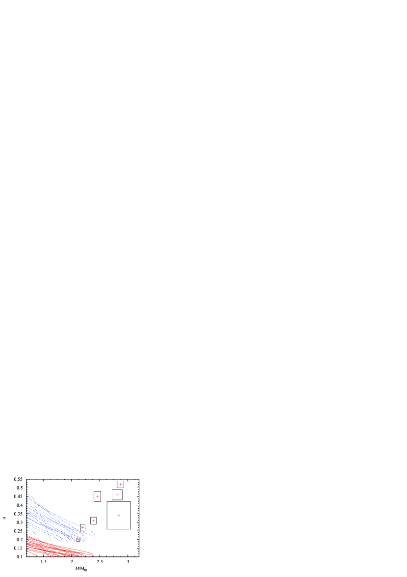
Fig. 1: Hartle–Thorne models of neutron stars with rotation frequency $f_{\mathrm{rot}}\sim 290\,\mathrm{Hz}$ (red) and $f_{\mathrm{rot}}\sim 580\,\mathrm{Hz}$ (blue), for a variety of EoS considered in Urbanec et al. (2013): SkT5, Sk0’, Sk0, SLy4, Gs, SkI2, SkI5, SGI, SV – Skyrme equations (Stone et al. 2003), UBS equation (Urbanec et al. 2010a), FPS equation (Lorenz et al. 1993), APR (Akmal et al. 1998), BBB2 equation (Baldo et al. 1997), BPAL12 equation (Bombaci 1995), BalbN1H1 equation (Balberg & Gal 1997), GlendNH3 equation (Glendenning 1985), APR2 equation (Akmal et al. 1998), Gandolfi equation (Gandolfi et al. 2010). Each equation of state applied in the Hartle–Thorne model predicts for a fixed rotational frequency a sequence of stable states represented by a curve in the $M$–$a$ plane; its final point indicates an instability. Clearly, all predicted values of the 4U 1636$-$53 neutron star spacetime parameters $M$, $a$ related to $f_{\mathrm{rot}}\sim 290\,\mathrm{Hz}$ are located outside the predictions of the Hartle–Thorne models.

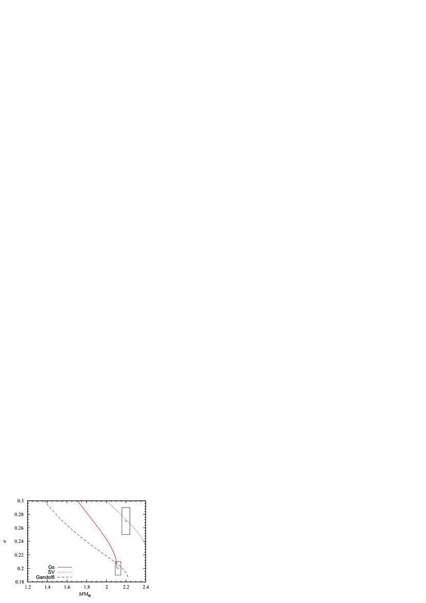
Fig. 2: Hartle–Thorne models of neutron stars with rotation frequency $f_{\mathrm{rot}}\sim 580\,\mathrm{Hz}$ are illustrated for the $a(M)$ dependencies related to the two best fits of the observational data by the RS model. The acceptable sequences of equilibrium configurations predicted by the Hartle–Thorne model are constructed for two equations of state (Skyrme SV EoS for RP1+RP variant, and Gandolfi EoS for the RP1+TP1 variant). Notice that the variant of the RS model predicting the lower parameters of $M=2.12\,\mathrm{M}_{\odot}$ and $a=0.20$ is also very close to the final state given by the sequence of equilibrium states predicted by the Skyrme Gs EoS, indicating possibility of an instability of the neutron star in the 4U 1636$-$53 system in near future.

We immediately see that no equation of state allows to construct a Hartle–Thorne model that can fit the RS model data, if we assume the rotational frequency of the 4U 1636$-$53 neutron star $f_{\mathrm{rot}}\sim 290\,\mathrm{Hz}$. For the rotational frequency $f_{\mathrm{rot}}\sim 580\,\mathrm{Hz}$, the Hartle–Thorne models give very interesting restrictions that are in significant agreement with results of the fitting the HF QPO data in the framework of the RS model. The Hartle–Thorne model based on the Skyrme equation of state SV meets with high precision the prediction of the RP1+RP version of the RS model that gives the best fit to the twin peak HF QPO data observed in the 4U 1636$-$53 source for the neutron star parameters $M\sim 2.20\,\mathrm{M}_{\odot}$ and $a\sim 0.27$. The Hartle–Thorne model based on the Gandolfi equation of state meets with high precision the prediction of the RP1+TP1 version of the RS model that gives the second best fit to the observational data of the twin HF QPOs in 4U 1636$-$53 for a neutron star having parameters $M\sim 2.12\,\mathrm{M}_{\odot}$ and $a\sim 0.20$. Notice that the variant of the RS model giving the second best fit is in accord with another version of the Skyrme equation of state (Gs) which predicts the neutron star with parameters $M\sim 2.11\,\mathrm{M}_{\odot}$ and $a\sim 0.20$. Such a result demonstrates that the 4U 1636$-$53 neutron star could be in a state very close to an instability, as the neutron star mass and spin indicated by the HF QPO data fitting procedure can correspond to the final state of the evolution of the neutron stars rotating with the frequency $f_{\mathrm{rot}}\sim 580\,\mathrm{Hz}$ and governed by the Skyrme equation of state Gs – see Figure 2. Predictions of all the other variants of the RS model are located in the $M$–$a$ plane at positions that are evidently out of the scope of all the equations of state considered in the present paper – we can expect that this is true even for all the variants of the presently known equations of state.

5.2 Parameters and the shape of the neutron star

Shape of isobaric surfaces $P=\mathrm{const.}$ and the shape of the neutron star surface $P=0$ are given by

$$r(P=\mathrm{const.},\theta)=r_{0}(P)+\xi_{0}(r_{0})+\xi_{2}(r_{0})P_{2}(\cos\theta)\,,$$ (13)

where $r_{0}$ is the spherical coordinate and functions $\xi_{0}$ and $\xi_{2}$ are given by the relations (Miller 1977)

$$\xi_{0}(r)=\frac{r[r-2m(r)]p_{0}}{4\pi r^{3}P+m(r)}\,,$$ (14)

$$\xi_{2}(r)=\frac{r[r-2m(r)]p_{2}}{4\pi r^{3}P+m(r)}$$ (15)

and

$$p_{2}(r)=-h_{2}(r)-\frac{1}{3}r^{2}\mathrm{e}^{-2\nu_{0}}\omega^{2}\,.$$ (16)

The calculations have been realized using the detailed set of equations presented in Miller (1977). Then equatorial and polar radii governing the surface shape of the rotating neutron star read

$$R_{\mathrm{eq}}=R_{0}(P)+\xi_{0}(R_{0})-\frac{1}{2}\xi_{2}(R_{0})\,,$$ (17)

$$R_{\mathrm{pol}}=R_{0}(P)+\xi_{0}(R_{0})+\xi_{2}(R_{0})\,.$$ (18)

The agreement of the Hartle–Thorne neutron star models based on the Skyrme and Gandolfi equations of state with two best fits of the observational data of twin HF QPOs observed in the source 4U 1636$-$53 enables to predict in detail properties of the neutron star in this source. Namely, we are able to find along with the two known parameters, mass $M$ and spin $a$, also the radius in the equatorial plane $R(\theta=\pi/2)$ and along the symmetry axis $R(\theta=0)$ and whole the shape of the neutron star surface, the moment of inertia $I$, and quadrupole moment $Q$ and its dimensionless form $q=QM/J^{2}$. Then we can calculate also the parameter representing compactness of the neutron stars in dependence on the latitude

$$C_{\theta}=\frac{R(\theta)}{2M}.$$ (19)

We can consider the characteristic values of the compactness parameter related to the equatorial plane $\theta=\pi/2$ and the symmetry axis $\theta=0$. Here we give for simplicity the compactness parameter related to the basical, spherically symmetric model that is a starting point of the Hartle–Thorne models, given by

$$C_{0}=\frac{R_{0}}{2M_{0}}.$$ (20)

The results of the Hartle–Thorne model calculations for all three equations of state giving acceptable agreement with the data predicted by the RS model are presented in Table 3. For the Skyrme equation of state SV, and the Gandolfi equation of state, the neutron star parameters are given for the mass parameter corresponding to the mean value of the data fitting (Stuchlík et al. 2014). In the case of the Skyrme equation of state Gs, the mass parameter of the neutron star ($M\sim 2.11\,\mathrm{M}_{\odot}$) corresponds to the maximal value predicted by this equation of state, i.e., it gives the instability point of the neutron stars governed by this equation of state. This mass parameter is lower than the related mean value given by the data fitting, but it falls into the allowed range of the mass parameter.

Table 3: Parameters of neutron stars predicted by the selected equations of state giving Hartle–Thorne models compatible with the fitting of the twin HF QPOs observed in 4U 1636$-$53. The mass is fixed to the mean value given by the fitting procedure with exception of the Skyrme equation of state Gs where it corresponds to the final state indicating an instability. The spin predicted by the Hartle–Thorne model fits the range given by the error determined by the data fitting. All models predict very compact neutron stars with low value of the parameter $q/a^{2}$.

EoS	$M$ $[\mathrm{M}_{\odot}]$	$R_{\mathrm{eq}}$ $[\mathrm{km}]$	$a$	$q$	$q/a^{2}$	$R_{0}/(2M_{0})$
Gandolfi	2.12	10.75	0.205	0.0723	1.71	1.72
Gs	2.11	10.84	0.201	0.0676	1.68	1.75
SV	2.20	13.41	0.272	0.1940	2.60	2.07

6 Self-consistency test by the Hartle–Thorne geometry

Assuming that the external geometry of the 4U 1636$-$53 neutron star can be approximated by the Kerr geometry, we have found that the two most precise variants of the RS model can be fitted by realistic EoS applied in the Hartle–Thorne model of slowly rotating neutron stars. For the RP1+RP variant, the Skyrme SV EoS predicts $M\sim 2.20\,\mathrm{M}_{\odot}$, $a\sim 0.272$, $q/a^{2}\sim 2.60$. For the RP1+TP1 variant, the Gandolfi EoS predicts $M\sim 2.12\,\mathrm{M}_{\odot}$, $a\sim 0.205$, $q/a^{2}\sim 1.71$; for this RS variant, also the Skyrme Gs EoS gives acceptable values of $M\sim 2.11\,\mathrm{M}_{\odot}$, $a\sim 0.201$, $q/a^{2}\sim 1.68$, however, this estimated mass parameter is at the maximum allowed mass for the EoS.

We have to realize now a self-consistency test of the Kerr geometry approximation applied in fitting the observational data. We have to check, if fitting the observational data by the $\chi^{2}$-test using the orbital and epicyclic frequencies related to the Hartle–Thorne geometry with parameters $M,\,a,\,q$ governed by the acceptable EoS gives results comparable or better than the fitting based on the assumption of the Kerr geometry approximation. We realize the self-consistency test in the following three steps.

First, we characterize the sequence of states given by the Hartle–Thorne model for the acceptable EoS and the rotational frequency of the neutron star $f_{\mathrm{rot}}=580\,\mathrm{Hz}$ – see Figure 3. The free parameter is the mass $M$ and we represent the sequence of the states by the functions $a(M)$ and $q/a^{2}(M)$. For each considered EoS we give the Hartle–Thorne model for $M>1.2\,\mathrm{M}_{\odot}$, and we follow the sequence of allowed neutron star states to the limiting values of the parameters $M,\,a,\,q/a^{2}$ corresponding to the maximal allowed mass for the considered EoS. For each of the EoS, the closest approach of the Hartle–Thorne model to the Kerr geometry occurs for the maximal mass allowed by given EoS. We can see that closest approach to the Kerr geometry is allowed for the Hartle–Thorne model based on the Gandolfi EoS, enabling the lowest value of $q/a^{2}\sim 1.5$ for $M_{\mathrm{max}}\sim 2.24\,\mathrm{M}_{\odot}$. On the other hand, the largest difference from the Kerr geometry approximation are expected for the Skyrme SV model with the lowest value of $q/a^{2}\sim 1.9$ – the maximal mass is highest for this EoS, reaching $M_{\mathrm{max}}\sim 2.4\,\mathrm{M}_{\odot}$.

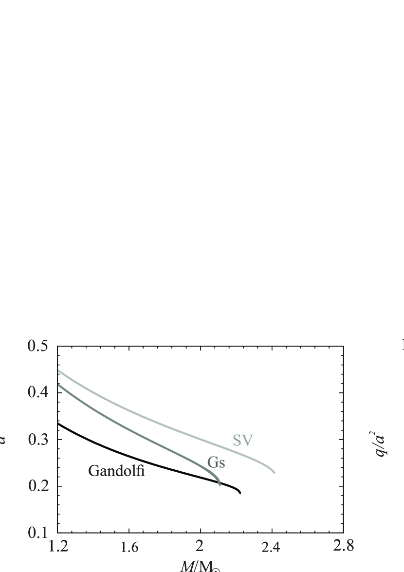
Fig. 3: Sequence of the Hartle–Thorne spacetime parameters implied by the Gandolfi, Skyrme Gs and Skyrme SV EoS for the rotational frequency $f_{\mathrm{rot}}=580\,\mathrm{Hz}$. Left: Spin ($a$) as a function of mass ($M$). Right: Reduced quadrupole moment ($q/a^{2}$) as a function of mass ($M$). All sequences are constructed for the mass interval $1.2\,\mathrm{M}_{\odot}<M<M_{\mathrm{max}}$.

Second, we define the orbital and epicyclic radial and vertical frequencies of the quasicircular geodesic motion in the Hartle–Thorne geometry, $\nu_{\mathrm{K}}(r;M,a,q)$, $\nu_{r}(r;M,a,q)$, $\nu_{\theta}(r;M,a,q)$ (Abramowicz et al. 2003; Török et al. 2008b). For completeness, we give the explicit expressions for the frequencies in the Appendix.

Third, using the Hartle–Thorne orbital and epicyclic frequencies, we repeat the least-square ($\chi^{2}$-test) fitting procedure for the same sample of the observational data in the 4U 1636$-$53 atoll source as those considered in our previous paper (Stuchlík et al. 2014). For the self-consistency test, we study only the two selected variants of the RS model, RP1+RP and RP1+TP1, along the sequences of the neutron star parameters $M,\,a,\,q$ related to the allowed EoS and the rotational frequency of the neutron star.

The results of the fitting procedure are given in Figure 4 for the RP1+RP variant of the RS model and the Skyrme SV EoS. Along with the fitting based on the Hartle–Thorne geometry, we repeat for comparison also the results obtained under the Kerr approximation of the neutron star external spacetime. The fitting procedure implies the best fit $\chi^{2}=101$; in comparison to the best fit based on the Kerr approximation ($\chi^{2}=55$, $M\sim 2.20\,\mathrm{M}_{\odot}$, $a\sim 0.272$), the mass parameter is shifted to lower value of $M\sim 2.11\,\mathrm{M}_{\odot}$, and higher value of spin $a\sim 0.286$. Moreover, at the values of mass and spin predicted by the Kerr approximation (when $\chi^{2}=55$, Stuchlík et al. 2014), the Hartle–Thorne geometry implies $\chi^{2}>1000$. Such a large discrepancy is caused by relatively large value of the parameter $q/a^{2}\sim 3$ when large errors of the Kerr approximation are expected. The resulting value of the Hartle–Thorne best fit, $\chi^{2}=101$, is too high in comparison with the Kerr approximation value, $\chi^{2}=55$, and we can conclude that the RP1+RP variant of the RS model is not satisfying the self-consistency test.

For the RP1+TP1 variant of the RS model and the Gandolfi EoS, the results of the fitting procedure are presented in Figure 5. We again give for comparison the results of the best fit obtained for the Kerr geometry approximation ($\chi^{2}=61$, $M\sim 2.12\,\mathrm{M}_{\odot}$, $a\sim 0.205$). The best fit based on the Hartle–Thorne geometry gives for the Gandolfi EoS $\chi^{2}=64$, a slight decrease of the mass parameter to $M=2.10\,\mathrm{M}_{\odot}$ and a very slight increase of the spin parameter to $a=0.208$. Therefore, we can conclude that the RP1+TP1 model with the Gandolfi EoS satisfies the self-consistency test, as both precision of the fit and the estimate of the neutron star parameters are in very good agreement with the predictions of the Kerr approximation used in the fitting procedure. The precision of the mass estimate is on the level of one percent. The best fit parameter $q/a^{2}=1.77$ is low enough to enable the high coincidence of predictions of the Hartle–Thorne geometry and the Kerr approximation.

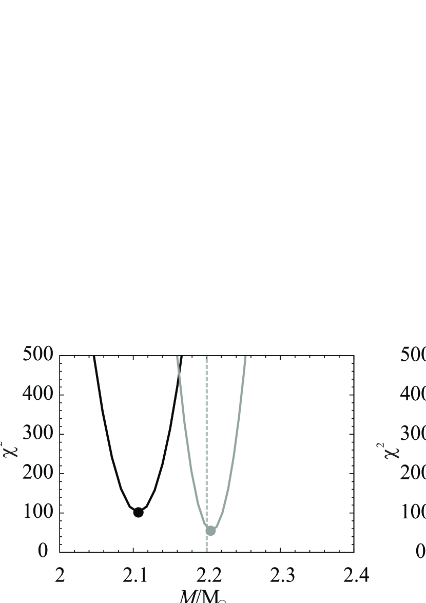
Fig. 4: The results of the fitting procedure for the RP1+RP variant of the RS model and the Skyrme SV EoS. $\chi^{2}$ dependency on $M$ (left), $a$ (middle), and $q/a^{2}$ (right). The gray curves correspond to the Kerr approximation. Dashed lines correspond to values of $M$ and $a$ from Table 3.

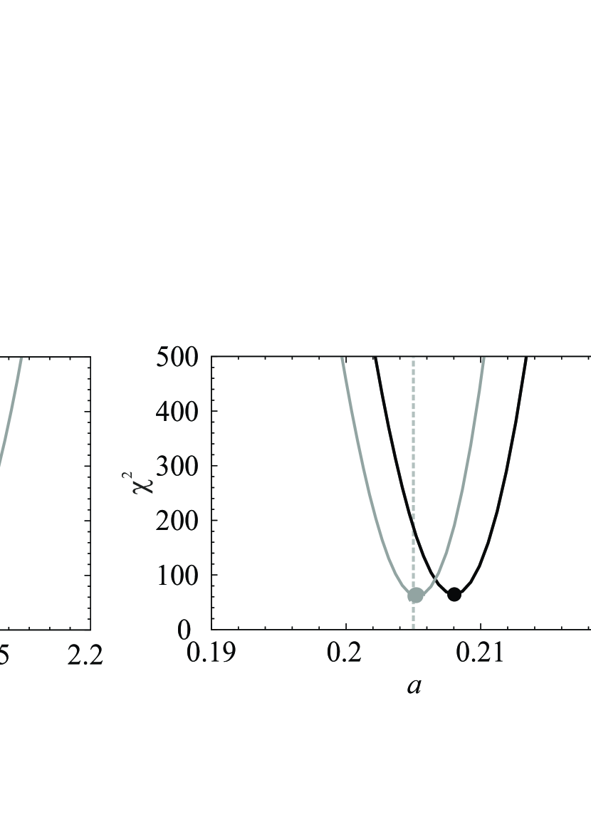
Fig. 5: The results of the fitting procedure for the RP1+TP1 variant of the RS model and the Gandolfi EoS. $\chi^{2}$ dependency on $M$ (left), $a$ (middle) and $q/a^{2}$ (right). The gray curves correspond to the Kerr approximation. Dashed lines correspond to values of $M$ and $a$ from Table 3.

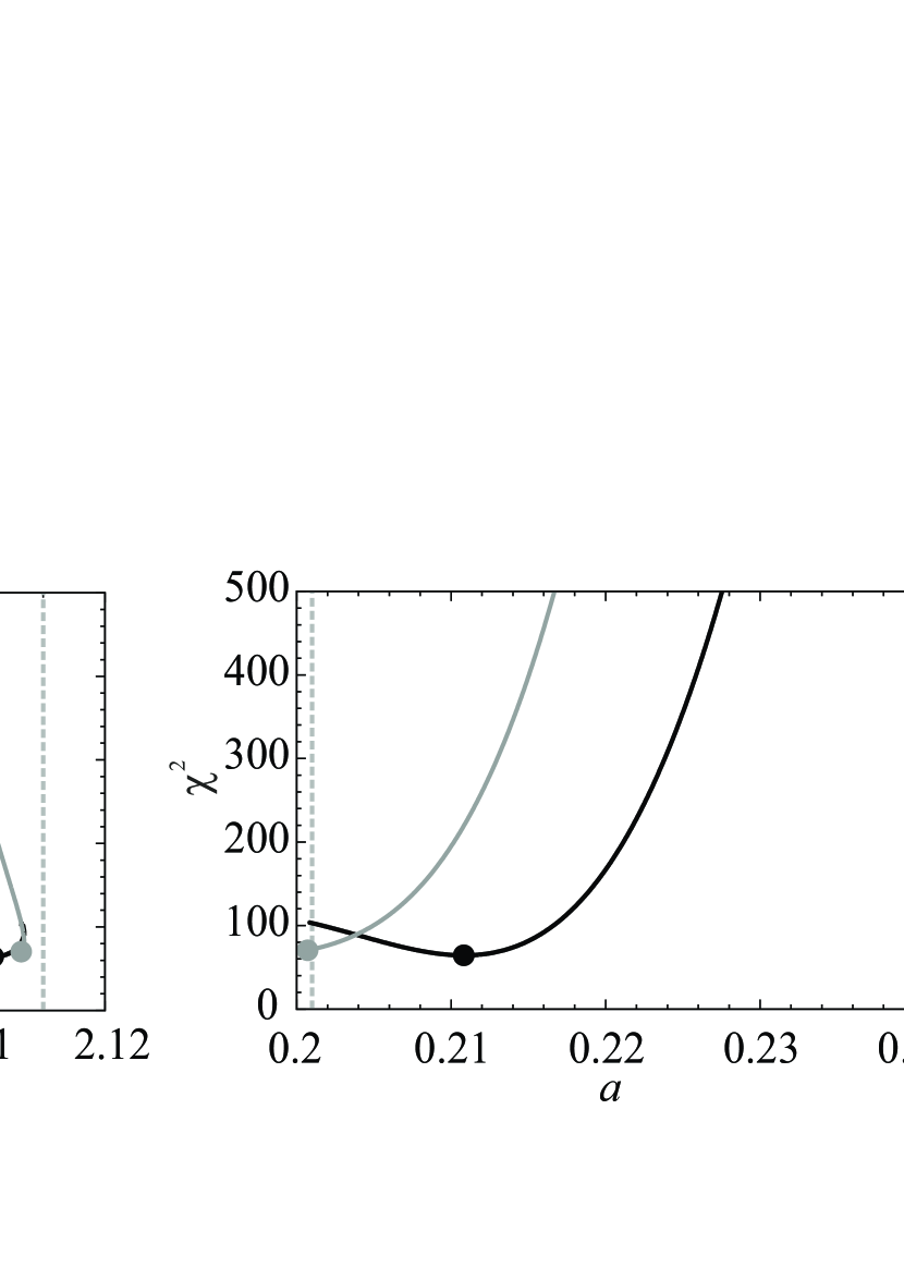
Fig. 6: The results of the fitting procedure for the RP1+TP1 variant of the RS model and the Gs EoS. $\chi^{2}$ dependency on $M$ (left), $a$ (middle) and $q/a^{2}$ (right). The gray curves correspond to the Kerr approximation. Dashed lines correspond to values of $M$ and $a$ from Table 3.

For the RP1+TP1 variant of the RS model and the Skyrme Gs EoS, the results of the fitting procedure are presented in Figure 6. We again give for comparison the results of the best fit obtained for the Kerr geometry approximation ($\chi^{2}=61$, $M\sim 2.12\,\mathrm{M}_{\odot}$, $a\sim 0.201$); however, for this EoS the maximal allowed mass ($M\sim 2.11\,\mathrm{M}_{\odot}$) is slightly lower than the Kerr approximation estimate. The best fit based on the Hartle–Thorne geometry gives for the Skyrme Gs EoS $\chi^{2}=64$, and a slight decrease of the mass parameter to $M=2.10\,\mathrm{M}_{\odot}$, still very close to the maximal allowed mass for this EOS, and a slight increase of the spin parameter to $a=0.211$. Therefore, we can conclude that the RP1+TP1 model with the Skyrme Gs EoS satisfies the self-consistency test, as both precision of the fit and the estimate of the neutron star parameters are in very good agreement with the predictions of the Kerr approximation. The precision of the mass estimate is on the level of one percent again. At the best fit, the parameter $q/a^{2}=1.83$ is still low enough to enable the high coincidence of predictions of the Hartle–Thorne geometry and the Kerr approximation. However, the predicted mass of the neutron star is very close to the maximum related to the Skyrme Gs EoS, bringing some doubts on the applicability of this EoS for the source 4U 1636$-$53; if the Skyrme Gs EoS is the proper one, than we could expect some strong instability of this source in near future.

The results of the $\chi^{2}$-test realized for the external Hartle–Thorne geometry with parameters governed by the acceptable EoS are summarized in Table 4. These results give the self-consistency test of the results obtained due to the assumption of Kerr approximation of the neutron star external spacetime. We can see that only the RP1+TP1 variant of the RS model can be considered as surviving the self-consistency test. Moreover, the Gandolfi EoS can be considered as the most plausible one in explaining the fitting of observational data related to the twin HF QPOs observed in the 4U 1636$-$53 source. Notice that the best fits implied by the Hartle–Thorne geometry give in all considered cases $\chi^{2}$ value that is higher (worse fit) than in the case of the fits based on the Kerr approximation. Of course, we could obtain better fits by the Hartle–Thorne geometry for other values of the neutron star parameters. But in such a case, the fits have to be related to the parameters $M,\,a,\,q$ considered as free parameters, while in our case the spacetime parameters were confined by the chosen EoS and the observed rotation frequency of the source. Therefore, we cannot exclude that in future an EoS will be discovered that will enable to obtain better fit to the observational data than those presented in our paper. However, we can note that all EoS considered in our paper give fits worse than those implied by the Gandolfi EoS.

Table 4: Results of the $\chi^{2}$-test realized for the external Hartle–Thorne geometry with parameters governed by the acceptable EoS.

EoS	Models	$M$ $[\mathrm{M}_{\odot}]$	$a$	$q/a^{2}$	$\chi^{2}$
Gandolfi	RP1+TP1	2.10	0.208	1.77	64
Gs	RP1+TP1	2.10	0.211	1.83	64
SV	RP1+RP	2.11	0.286	2.99	101

7 Discussion

The atoll source 4U 1636$-$53 seems to be one of the best test beds for both the models of strong gravity phenomena and the microphysics determining equations of state governing the internal structure and exterior of neutron stars. This is due to simultaneous availability of relatively good observational data of the HF QPOs occurring in the innermost parts of the accretion disc where the extremely strong gravity is relevant, enabling thus to put precise restrictions on the neutron star external spacetime parameters in the framework of the RS model, and the knowledge of the rotational frequency of the neutron star that enables a precise modeling of the internal and external structure of rotating neutron stars in the framework of the Hartle–Thorne theory, for whole variety of the equations of state. Strong restrictions on the acceptable versions of the RS model can be obtained, because the precise knowledge of the rotational frequency of the neutron star implies a narrow evolution line for the Hartle–Thorne models in the $M$–$a$ plane that has to be adjusted to relatively precisely determined points in the $M$–$a$ plane predicted by the acceptable variants of the RS model of the observed HF QPOs.

The RS model can be well tested for the atoll source 4U 1636$-$53 since this source demonstrates two resonant radii in the observational data. For all relevant pairs of the oscillatory frequency relations of the RS model, the range of allowed values of the mass and dimensionless spin of the neutron star at 4U 1636$-$53 has been given in Stuchlík et al. (2012). The most promising frequency pairs predicting the range of the 4U 1636$-$53 neutron star mass and spin in accord with neutron star structure theory were tested by fitting the frequency relation pairs to the observational data on the HF QPOs separated into two parts related to the pair of frequency relations – only the frequency relations containing geodesic orbital and epicyclic frequencies, or some combinations of these frequencies, were considered (Stuchlík et al. 2014). Nevertheless, it should be noted that the cause of the switch of the pairs of the oscillatory modes is not tied to the resonant phenomena related to the oscillations governed by the frequencies of the geodesic motion. The switch can be related, e.g., to the influence of the magnetic field of the neutron star and after the switch the Alfvén wave model can be relevant (Zhang et al. 2006). However, limiting the study to the resonant phenomena and frequencies of the geodesic origin, the number of free parameters of the model is restricted to the mass $M$ and dimensionless spin $a$ of the neutron star, as we are able to demonstrate that the predicted mass of the neutron star is large enough to guarantee with high precision independence of the geodesic frequencies on the quadrupole moment of the neutron star and applicability of the Kerr approximation in decribing the neutron star external geometry (Urbanec et al. 2013). Inclusion of the non-geodesic oscillation modes and non-resonant causes of the switch is postponed to future studies and could be relevant for some other sources containing neutron stars.

The fitting procedure realized in the framework of the RS model is shown to be more precise by almost one order in comparison to the standard fitting based on the individual frequency relations that were used in pairs in the RS model (Stuchlík et al. 2014). For example, the fitting by the standard RP model predicts the best fit along the mass–spin relation $M(a)=M_{0}\left[1+0.75(a+a^{2})\right]$ with rather poor maximal precision of the $\chi^{2}$ test given by $\chi^{2}\sim 350$ and $\chi^{2}/\mathrm{dof}\sim 16$; the other frequency relations give comparable poor precision (Török et al. 2012). Similar results with poor precision were obtained also for models with frequency relations of non-geodesic origin (Lin et al. 2011). On the other hand, the best fit obtained for the RS model with frequency relation pair RP1+RP gives $\chi^{2}\sim 55$ and $\chi^{2}/\mathrm{dof}\sim 2.6$ that is quite acceptable due to the character of the data distribution (Török et al. 2012). The RP1+TP1 version of the RS model predicts the second best fit with precision that is given by $\chi^{2}\sim 61$ and $\chi^{2}/\mathrm{dof}\sim 2.9$.

Testing the RS model by the Hartle–Thorne theory with fixed rotation frequency and a variety of equations of state brings another efficient selection of the variants of the RS model. The results are illustrated by Figures 1 and 2 and clearly demonstrate that only the two variants of the RS model giving the best results of the data fitting are acceptable by the Hartle–Thorne models of the neutron star structure, if the rotation frequency $f_{\mathrm{rot}}\sim 580\,\mathrm{Hz}$. The RP1+RP version of the RS model predicts mean values of mass $M\sim 2.20\,\mathrm{M}_{\odot}$ and spin $a\sim 0.27$ and these are the data that can be met precisely by the Hartle–Thorne models – namely for the Skyrme equation of state SV. The RP1+TP1 version of the RS model predicts the mean values of mass $M\sim 2.12\,\mathrm{M}_{\odot}$ and spin $a\sim 0.20$. This mass and spin can be explained by the Hartle–Thorne model with the Gandolfi equation of state. It is interesting that the prediction of the Hartle–Thorne model based on the Skyrme equation of state Gs enters the allowed range of the mass and spin parameters given by the RP1+TP1 version of the RS model, although it does not reach the mean value of the mass parameter, as demonstrated in Figure 2. If this equation of state is the real one, the neutron star at the source 4U 1636$-$53 has to be in a state very close to instability leading to some form of collapse and dramatic observational phenomena. Mass and spin of the neutron star predicted by the other versions of the RS model acceptable due to the data fitting are completely out of the range of the $M$–$a$ dependencies predicted by the Hartle–Thorne model for the whole variety of available equations of state.

In the special situations related to accreting neutron stars with near-maximum masses, the Kerr metric can be well applied in calculating the orbital and epicyclic geodesic frequencies, as has been done in the present paper. It should be stressed that the neutron star mass and spin parameters predicted by the two relevant findings of frequency pairs are in agreement with the assumption of near-maximum masses of the neutron stars – see Figure 2. For each acceptable equation of state and the observed rotation frequency of the neutron star, the Hartle–Thorne model has been constructed, giving thus not only mass $M$ and spin $a$, but also the dimensionless quadrupole moment $q$ and other characteristics as the equatorial radius and the compactness. The detailed results of the Hartle–Thorne model obtained for the three equations of state that can be in the play are shown in Table 3. The results clearly demonstrate that in all three cases we obtain a very compact neutron star, especially for the Gandolfi and Skyrme Gs equations of state, related to the second best fit with mass parameter $M\sim 2.12\,\mathrm{M}_{\odot}$ and spin $a=0.2$, having radius $R\sim 3.5\,M$. The spin exactly predicted by the Hartle–Thorne model is slightly overcoming the mean value of the spin of the data fitting of the RS model, but it belongs to the allowed range. The parameter $q/a^{2}\sim 1.7$ corresponds to the external Hartle–Thorne spacetime that is very close to the Kerr spacetime.

The self-consistency test of the RP1+TP1 variant of the RS model by the Hartle–Thorne geometry, related to the Gandolfi EoS, confirms this choice, since the results of the $\chi^{2}$-test are very close to those obtained due to the test by the Kerr geometry approximation – both for the value of $\chi^{2}$ at the best fit, and the close values of the mass and spin spacetime parameters. Similar results are obtained by the self-consistency test for the Hartle–Thorne model related to the Skyrme Gs EoS. However, the test confirms also the conclusion that the estimated mass has to be very close to the maximum allowed by the EoS, lowering thus the potential relevance of this EoS for the 4U 1636$-$53 neutron star.

For the RP1+RP variant of the RS model, the Hartle–Thorne model using the Skyrme SV EoS, related to the neutron star with mass $M\sim 2.20\,\mathrm{M}_{\odot}$, the spin is also predicted with the high precision $a=0.272$, but the neutron star is not so extremely compact, having radius $R\sim 4.1\,M$; the parameter $q/a^{2}\sim 2.6$ is too high to approve the application of the Kerr geometry in description of the Hartle–Thorne external spacetime. In fact, the self-consistency test by the Hartle–Thorne geometry predicts the best fit with $\chi^{2}$ being too high (twice the estimate due to the fitting procedure using the Kerr approximation) to imply relevance of this variant for the chosen EoS. For this reason the RP1+RP variant of the RS model can be considered to be excluded by the self-consistence test.

8 Conclusions

We can conclude that there is a strong synergy effect of our approach. As expected, the equations of state applied in the Hartle–Thorne model of neutron stars fully exclude a lot of variants of the RS model that could be acceptable due to the fitting procedure to the HF QPO data observed in the 4U 1636$-$53 source. Moreover, the results of the RS model allow for the rotation frequency of the 4U 1636$-$53 neutron star $f_{\mathrm{rot}}=580\,\mathrm{Hz}$, but fully exclude the possibility of $f_{\mathrm{rot}}=290\,\mathrm{Hz}$.

The restrictions work effectively in the opposite direction too – the results of the RS model put significant restrictions on the relevance of the equations of state. The crucial point is that the self-consistency test by fitting the observational data by the RS model with the orbital and epicyclic frequencies in the Hartle–Thorne geometry related to the acceptable EoS excludes one of the variants of the RS model predicted by the fitting under the Kerr approximation of the neutron star external geometry, and also the corresponding EoS. In fact, we have shown that the RP1+RP variant of the RS model along with the Skyrme SV EoS connected to this variant are excluded by the self-consistency test giving high value of $\chi^{2}$ at the best fit. It is interesting that this happens for the variant of the RS model giving the best fit to the data of twin HF QPOs when the Kerr approximation of the oscillatory frequencies has been used.

On the other hand, the RP1+TP1 variant of the RS model related to a very stiff Gandolfi EoS goes successfully through the self-consistency test by the Hartle–Thorne geometry. In this case, the resulting best fit gives $\chi^{2}=64$ that is well comparable to the result obtained for the Kerr approximation ($\chi^{2}=61$). The resulting neutron star parameters ($M\sim 2.10\,\mathrm{M}_{\odot}$, $a\sim 0.208$, and $q/a^{2}\sim 1.77$) are also very close to those obtained in the Kerr approximation, demonstrating errors of one percent. Moreover, the Skyrme Gs EoS used in the self-consistency test by the Hartle–Thorne geometry gives also acceptable results, implying a possibility of the 4U 1636$-$53 neutron star being near the marginally stable state with mass $M\sim 2.11\,\mathrm{M}_{\odot}$. Of course, the vicinity of an instability of the neutron star puts some doubts on the applicability of the Skyrme Gs EoS.

We can conclude that in the framework of the Hartle–Thorne theory the EoS imply strong restriction on the RS model of the twin HF QPOs observed in the atoll source 4U 1636$-$53. In fact only the RP1+TP1 variant of the RS model satisfies the self-consistency test. Moreover, it seems that there is only one EoS, namely the Gandolfi EoS that can be considered as a fully realistic choice in the framework of the modelling the twin HF QPOs. The self-consistency test also demonstrates that the Kerr approximation of the neutron star external geometry gives very precise estimates for very compact neutron stars having sufficiently low values of the parameter $q/a^{2}<2$.

It was shown that observations of the twin HF QPOs provide tests on equation of state that put limits on the gravitational mass, and the spin that is linearly related to the moment of inertia of the neutron star. This could provide another test of the equations of state that allow for existence of neutron stars with $M>2.0\,\mathrm{M}_{\odot}$.

For the equations of state acceptable by the RS model we can determine also the quadrupole moment and the shape of the neutron star surface governed by the equatorial and polar radii. These quantities have to enter other strong gravity tests of the 4U 1636$-$53 neutron star spacetime parameters predicted by the twin HF QPOs, e.g., the profiled spectral lines generated at the neutron star surface or at its accretion disc. We believe that such tests could confirm or exclude one of the two EoS implied by the acceptable variant of the RS model.

Of course, it will be very important to test the RS model of the twin HF QPOs and all its consequences for some other neutron star system. We have to check, if the same variant of the RS model, and the same EoS in the Hartle–Thorne theory of the neutron stars could be relevant. However, no source similar to the 4U 1636$-$53 neutron star system has been observed. Such sources have to demonstrate sufficiently extended range of the twin HF QPOs and an indication of two clusters of the observational data that could be related to different models of twin HF QPOs that could be switched at a resonant point. Simultaneously, we have to know the rotation frequency of the neutron star.

Acknowledgements. The authors acknowledge the internal grants of the Silesian University in Opava FPF SGS/11,23/2013. ZS acknowledges the Albert Einstein Center for Gravitation and Astrophysics supported by the Czech Science Foundation grant No. 14-37086G. MU and GT acknowledge the support of the Czech grant GAČR 209/12/P740.

Appendix. Orbital and epicyclic frequencies in Hartle–Thorne geometry

Circular and epicyclic geodesic motion in the Hartle–Thorne geometry has been studied in Abramowicz et al. (2003); Török et al. (2008b, 2015). Here we only present the expressions for the orbital (Keplerian) frequency and the radial and vertical epicyclic frequencies as given in Török et al. (2008b). Alternative, but equivalent, expressions can be found in Boshkayev et al. (2014).

The Keplerian frequency is determined by the relations

$$\nu_{\mathrm{K}}(r;M,a,q)=\frac{c^{3}}{2\pi GM}\frac{1}{r^{3/2}}\left[1-\frac{a}{r^{3/2}}+a^{2}E_{1}(r)+qE_{2}(r)\right],$$ (21)

where

$$E_{1}(r) = [48-80r+4r^{2}-18r^{3}+40r^{4}+10r^{5}+15r^{6}-15r^{7}]$$

$$(16(r-2)r^{4})^{-1}+\frac{15(r^{3}-2)}{32}\ln\left(\frac{r}{r-2}\right),$$

$$E_{2}(r) = \frac{5(6-8r-2r^{2}-3r^{3}+3r^{4})}{16(r-2)r}-\frac{15(r^{3}-2)}{32}\ln\left(\frac{r}{r-2}\right).$$ (22)

The radial epicyclic frequency $\nu_{r}$ and the vertical epicyclic frequency $\nu_{\theta}$ are given by the relations

$$\nu_{r}^{2}(r;M,a,q) = \left(\frac{c^{3}}{2\pi GM}\right)^{2}\frac{(r-6)}{r^{4}}[1+aF_{1}(r)-a^{2}F_{2}(r)-qF_{3}(r)],$$ (23)

$$\nu_{\theta}^{2}(r;M,a,q) = \left(\frac{c^{3}}{2\pi GM}\right)^{2}\frac{1}{r^{3}}[1-aG_{1}(r)+a^{2}G_{2}(r)+qG_{3}(r)],$$ (24)

where

$$F_{1}(r) = \frac{6(r+2)}{r^{3/2}(r-6)},$$

$$F_{2}(r) = [8r^{4}(r-2)(r-6)]^{-1}[384-720r-112r^{2}-76r^{3}$$

$$-138r^{4}-130r^{5}+635r^{6}-375r^{7}+60r^{8}]+A(r),$$

$$F_{3}(r) = \frac{5(48+30r+26r^{2}-127r^{3}+75r^{4}-12r^{5})}{8r(r-2)(r-6)}-A(r),$$

$$A(r) = \frac{15r(r-2)(2+13r-4r^{2})}{16(r-6)}\ln\left(\frac{r}{r-2}\right),$$

$$G_{1}(r) = \frac{6}{r^{3/2}},$$

$$G_{2}(r) = [8r^{4}(r-2)]^{-1}[48-224r+28r^{2}+6r^{3}-170r^{4}+295r^{5}$$

$$-165r^{6}+30r^{7}]-B(r),$$

$$G_{3}(r) = \frac{5(6+34r-59r^{2}+33r^{3}-6r^{4})}{8r(r-2)}+B(r),$$

$$B(r) = \frac{15(2r-1)(r-2)^{2}}{16}\ln\left(\frac{r}{r-2}\right).$$

References

- Abramowicz et al. (2005) Abramowicz, M. A., Barret, D., Bursa, M., et al. 2005, Astron. Nachr., 326, 864
- Abramowicz et al. (2003) Abramowicz, M. A. and Almergren, G. J. E. and Kluźniak, W. and Thampan, A. V. 2003, arXiv:gr-qc/0312070
- Akmal & Pandharipande (1997) Akmal, A. & Pandharipande, V. R. 1997, Phys. Rev. C, 56, 2261
- Akmal et al. (1998) Akmal, A., Pandharipande, V. R., & Ravenhall, D. G. 1998, Phys. Rev. C, 58, 1804
- Antoniadis et al. (2013) Antoniadis, J., Freire, P. C. C., Wex, N., et al. 2013, Science, 340, 448
- Bakala et al. (2010) Bakala, P., Šrámková, E., Stuchlík, Z., & Török, G. 2010, Classical Quantum Gravity, 27, 045001
- Balberg & Gal (1997) Balberg, S. & Gal, A. 1997, Nuclear Physics A, 625, 435
- Baldo et al. (1997) Baldo, M., Bombaci, I., & Burgio, G. F. 1997, A&A, 328, 274
- Barret et al. (2005a) Barret, D., Olive, J.-F., & Miller, M. C. 2005a, MNRAS, 361, 855
- Barret et al. (2005b) Barret, D., Olive, J.-F., & Miller, M. C. 2005b, Astron. Nachr., 326, 808
- Belloni et al. (2007) Belloni, T., Homan, J., Motta, S., Ratti, E., & Méndez, M. 2007, MNRAS, 379, 247
- Bombaci (1995) Bombaci, I. 1995, in “Perspectives on Theoretical Nuclear Physics”, ed. I. Bombaci, A. Bonaccorso, A. Fabrocini, et al., 223–237
- Bonazzola et al. (1998) Bonazzola, S., Gourgoulhon, E., & Marck, J.-A. 1998, Phys. Rev. D, 58, 104020
- Boshkayev et al. (2014) Boshkayev, K., Bini, D., Rueda, J., Geralico, A., Muccino, M. & Siutsou, I. 2014, Gravitation and Cosmology, 20, 233
- Boutloukos et al. (2006) Boutloukos, S., van der Klis, M., Altamirano, D., et al. 2006, ApJ, 653, 1435
- Bursa (2005) Bursa, M. 2005, in “Proceedings of RAGtime 6/7: Workshops on black holes and neutron stars”, Opava, 16–18/18–20 September 2004/2005, ed. S. Hledík & Z. Stuchlík (Opava: Silesian University in Opava), 39–45
- Chandrasekhar & Miller (1974) Chandrasekhar, S. & Miller, J. C. 1974, MNRAS, 167, 63
- Colpi & Miller (1992) Colpi, M. & Miller, J. C. 1992, ApJ, 388, 513
- Cremaschini & Stuchlík (2013) Cremaschini, C. & Stuchlík, Z. 2013, Phys. Rev. E, 87, 043113
- Demorest et al. (2010) Demorest, P. B., Pennucci, T., Ransom, S. M., Roberts, M. S. E., & Hessels, J. W. T. 2010, Nature, 467, 1081
- Farhi & Jaffe (1984) Farhi, E. & Jaffe, R. L. 1984, Phys. Rev. D, 30, 2379
- Gandolfi et al. (2010) Gandolfi, S., Illarionov, A. Y., Fantoni, S., et al. 2010, MNRAS, 404, L35
- Glendenning (1985) Glendenning, N. K. 1985, ApJ, 293, 470
- Gondek-Rosińska et al. (2014) Gondek-Rosińska, D., Kluźniak, W., Stergioulas, N., & Wiśniewicz, M. 2014, Phys. Rev. D, 89, 104001
- Haensel et al. (1986) Haensel, P., Zdunik, J. L., & Schaefer, R. 1986, A&A, 160, 121
- Hartle (1967) Hartle, J. B. 1967, ApJ, 150, 1005
- Hartle & Thorne (1968) Hartle, J. B. & Thorne, K. 1968, ApJ, 153, 807
- Horák et al. (2009) Horák, J., Abramowicz, M. A., Kluźniak, W., Rebusco, P., & Török, G. 2009, A&A, 499, 535
- Kato (2008) Kato, S. 2008, PASJ, 60, 111
- Kostić et al. (2009) Kostić, U., Čadež, A., Calvani, M., & Gomboc, A. 2009, A&A, 496, 307
- Kovář et al. (2008) Kovář, J., Stuchlík, Z., & Karas, V. 2008, Classical Quantum Gravity, 25, 095011, arXiv:0803.3155 [astro-ph]
- Lattimer & Prakash (2007) Lattimer, J. M. & Prakash, M. 2007, Phys. Rep., 442, 109
- Lin et al. (2011) Lin, Y.-F., Boutelier, M., Barret, D., & Zhang, S.-N. 2011, ApJ, 726, 74
- Lo & Lin (2011) Lo, K.-W. & Lin, L.-M. 2011, ApJ, 728, 12
- Lorenz et al. (1993) Lorenz, C. P., Ravenhall, D. G., & Pethick, C. J. 1993, Phys. Rev. Lett., 70, 379
- Miller (1977) Miller, J. C. 1977, MNRAS, 179, 483
- Miller et al. (1998) Miller, M. C., Lamb, F. K., & Psaltis, D. 1998, ApJ, 508, 791
- Montero & Zanotti (2012) Montero, P. J. & Zanotti, O. 2012, MNRAS, 419, 1507
- Mukherjee & Bhattacharyya (2012) Mukherjee, A. & Bhattacharyya, S. 2012, ApJ, 756, 55
- Mukhopadhyay (2009) Mukhopadhyay, B. 2009, ApJ, 694, 387
- Müller & Serot (1996) Müller, H. & Serot, B. D. 1996, Nuclear Physics A, 606, 508
- Müther et al. (1987) Müther, H., Prakash, M., & Ainsworth, T. L. 1987, Physics Letters B, 199, 469
- Pawar et al. (2013) Pawar, D. D., Kalamkar, M., Altamirano, D., et al. 2013, MNRAS, 433, 2436
- Perez et al. (1997) Perez, C. A., Silbergleit, A. S., Wagoner, R. V., & Lehr, D. E. 1997, ApJ, 476, 589
- Postnikov et al. (2010) Postnikov, S., Prakash, M., & Lattimer, J. M. 2010, Phys. Rev. D, 82, 024016
- Press et al. (2007) Press, W. H., Teukolsky, S. A., Vetterling, W. T., & Flannery, B. P. 2007, Numerical Recipes: The Art of Scientific Computing, 3rd edn. (Cambridge: Cambridge University Press), 1256
- Rhoades & Ruffini (1974) Rhoades, C. E. & Ruffini, R. 1974, Phys. Rev. Lett., 32, 324
- Sanna et al. (2012) Sanna, A., Méndez, M., Belloni, T., & Altamirano, D. 2012, poster presentation at IAU General Assembly XXVIII, 20–31 August 2012, Beijing, China
- Schee & Stuchlík (2009) Schee, J. & Stuchlík, Z. 2009, General Relativity and Gravitation, 41, 1795, arXiv:0812.3017 [astro-ph]
- Shi (2011) Shi, C. 2011, Research in Astronomy and Astrophysics, 11, 1327
- Stefanov (2014) Stefanov, I. Z. 2014, MNRAS, 444, 2178
- Steiner et al. (2010) Steiner, A. W., Lattimer, J. M., & Brown, E. F. 2010, ApJ, 722, 33
- Stella & Vietri (1998) Stella, L. & Vietri, M. 1998, ApJ, 492, L59
- Stella & Vietri (1999) Stella, L. & Vietri, M. 1999, Phys. Rev. Lett., 82, 17
- Stergioulas (2003) Stergioulas, N. 2003, Living Rev. Rel., 6, 3
- Stone et al. (2003) Stone, J. Ř., Miller, J. C., Koncewicz, R., Stevenson, P. D., & Strayer, M. R. 2003, Phys. Rev. C, 68, 034324
- Straub & Šrámková (2009) Straub, O. & Šrámková, E. 2009, Classical Quantum Gravity, 26, 055011, arXiv:0901.1635 [astro-ph.SR]
- Strohmayer & Markwardt (2002) Strohmayer, T. E. & Markwardt, C. B. 2002, ApJ, 577, 337
- Stuchlík & Kološ (2012) Stuchlík, Z. & Kološ, M. 2012, J. Cosmology Astropart. Phys., 10, 008, arXiv:1309.6879 [gr-qc]
- Stuchlík & Kološ (2014) Stuchlík, Z. & Kološ, M. 2014, Phys. Rev. D, 89, 065007
- Stuchlík & Kološ (2015) Stuchlík, Z. & Kološ, M. 2015, General Relativity and Gravitation, 47, 27
- Stuchlík & Kotrlová (2009) Stuchlík, Z. & Kotrlová, A. 2009, General Relativity and Gravitation, 41, 1305, arXiv:0812.5066 [astro-ph]
- Stuchlík et al. (2011) Stuchlík, Z., Kotrlová, A., & Török, G. 2011, A&A, 525, A82, arXiv:1010.1951 [astro-ph.HE]
- Stuchlík et al. (2012) Stuchlík, Z., Kotrlová, A., & Török, G. 2012, Acta Astron., 62, 389, arXiv:1301.2830 [astro-ph.HE]
- Stuchlík et al. (2013) Stuchlík, Z., Kotrlová, A., & Török, G. 2013, A&A, 552, A10, arXiv:1305.3552 [astro-ph.HE]
- Stuchlík et al. (2014) Stuchlík, Z., Kotrlová, A., Török, G., & Goluchová, K. 2014, Acta Astron., 64, 45
- Stuchlík & Schee (2012) Stuchlík, Z. & Schee, J. 2012, Classical Quantum Gravity, 29, 065002
- Stuchlík et al. (2007) Stuchlík, Z., Török, G., & Bakala, P. 2007, ArXiv e-prints
- Török (2009) Török, G. 2009, A&A, 497, 661, arXiv:0812.4751 [astro-ph]
- Török et al. (2005) Török, G., Abramowicz, M. A., Kluźniak, W., & Stuchlík, Z. 2005, A&A, 436, 1, arXiv:astro-ph/0401464
- Török & Stuchlík (2005) Török, G. & Stuchlík, Z. 2005, A&A, 437, 775, arXiv:astro-ph/0502127
- Török et al. (2008a) Török, G., Abramowicz, M. A., Bakala, P., et al. 2008a, Acta Astron., 58, 15, arXiv:0802.4070 [astro-ph]
- Török et al. (2008b) Török, G., Bakala, P., Stuchlík, Z., & Čech, P. 2008b, Acta Astron., 58, 1
- Török et al. (2010) Török, G., Bakala, P., Šrámková, E., Stuchlík, Z., & Urbanec, M. 2010, ApJ, 714, 748, arXiv:1008.0088 [astro-ph.HE]
- Török et al. (2012) Török, G., Bakala, P., Šrámková, E., et al. 2012, ApJ, 760, 138
- Török et al. (2015) Török, G., Goluchová, K., Urbanec, M., Šrámková, E., Adámek, K., Urbancová, G., Pecháček, T., Bakala, P., Stuchlík, Z., Horák, J., & Jurýšek, J. 2015. in “Proceedings of RAGtime: Workshops on black holes and neutron stars”, Opava, 2015, (Opava: Silesian University in Opava)
- Urbanec et al. (2010a) Urbanec, M., Běták, E., & Stuchlík, Z. 2010a, Acta Astron., 60, 149, arXiv:1007.3446 [astro-ph.SR]
- Urbanec et al. (2010b) Urbanec, M., Török, G., Šrámková, E., et al. 2010b, A&A, 522, A72, arXiv:1007.4961 [astro-ph.HE]
- Urbanec et al. (2013) Urbanec, M., Miller, J. C., & Stuchlík, Z. 2013, MNRAS, 433, 1903, arXiv:1301.5925 [astro-ph.SR]
- van der Klis (2006) van der Klis, M. 2006, in “Compact Stellar X-Ray Sources”, ed. W. H. G. Lewin & M. van der Klis (Cambridge: Cambridge University Press), 39–112
- Wang et al. (2013) Wang, D. H., Chen, L., Zhang, C. M., Lei, Y. J., & Qu, J. L. 2013, MNRAS, 435, 3494
- Witten (1984) Witten, E. 1984, Phys. Rev. D, 30, 272
- Zhang et al. (2006) Zhang, C. M., Yin, H. X., Zhao, Y. H., Zhang, F., & Song, L. M. 2006, MNRAS, 366, 1373