SImulator of GAlaxy Millimeter/submillimeter Emission (SÍGAME): the [Cii] $-$SFR relationship of massive z=2 main sequence galaxies

Abstract

We present SÍGAME simulations of the [Cii] $157.7\,{\rm\mu m}$ fine structure line emission from cosmological smoothed particle hydrodynamics (SPH) simulations of seven main sequence galaxies at $z=2$. Using sub-grid physics prescriptions the gas in our simulations is modeled as a multi-phased interstellar medium (ISM) comprised of molecular gas residing in giant molecular clouds, an atomic gas phase associated with photo-dissociation regions (PDRs) at the cloud surfaces, and a diffuse, ionized gas phase. Adopting logotropic cloud density profiles and accounting for heating by the local FUV radiation field and cosmic rays by scaling both with local star formation rate (SFR) volume density, we calculate the [Cii] emission using a photon escape probability formalism. The [Cii] emission peaks in the central $\mathrel{\raise 1.50696pt\hbox{$\scriptstyle<$}\kern-6.00006pt\lower 1.72218pt\hbox{{$\scriptstyle\sim$}}}1\,{\rm kpc}$ of our galaxies as do the SFR radial profiles, with most [Cii] ($\mathrel{\raise 1.50696pt\hbox{$\scriptstyle>$}\kern-6.00006pt\lower 1.72218pt\hbox{{$\scriptstyle\sim$}}}70\%$) originating in the molecular gas phase, whereas further out ($\mathrel{\raise 1.50696pt\hbox{$\scriptstyle>$}\kern-6.00006pt\lower 1.72218pt\hbox{{$\scriptstyle\sim$}}}2\,{\rm kpc}$), the atomic/PDR gas dominates ($\mathrel{\raise 1.50696pt\hbox{$\scriptstyle>$}\kern-6.00006pt\lower 1.72218pt\hbox{{$\scriptstyle\sim$}}}90\%$) the [Cii] emission, no longer tracing on-going star formation. Throughout, the ionized gas contribution is negligible ($\mathrel{\raise 1.50696pt\hbox{$\scriptstyle<$}\kern-6.00006pt\lower 1.72218pt\hbox{{$\scriptstyle\sim$}}}3\%$). The [Cii] luminosity vs. SFR ([Cii]-SFR) relationship, integrated as well as spatially resolved (on scales of $1\,{\rm kpc}$), delineated by our simulated galaxies is in good agreement with the corresponding relations observed locally and at high redshifts. In our simulations, the molecular gas dominates the [Cii] budget at ${\rm SFR}\mathrel{\raise 1.50696pt\hbox{$\scriptstyle>$}\kern-6.00006pt\lower 1.72218pt\hbox{{$\scriptstyle\sim$}}}20\,{\rm\mbox{$\rm{M}_{\odot}$}\,yr^{-1}}$ ($\mbox{$\Sigma_{\rm{SFR}}$}\mathrel{\raise 1.50696pt\hbox{$\scriptstyle>$}\kern-6.00006pt\lower 1.72218pt\hbox{{$\scriptstyle\sim$}}}0.5\,{\rm\mbox{$\rm{M}_{\odot}$}\,yr^{-1}\,kpc^{-2}}$), while atomic/PDR gas takes over at lower SFRs, suggesting a picture in which [Cii] predominantly traces the molecular gas in high-density/pressure regions where star formation is on-going, and otherwise reveals the atomic/PDR gas phase.

1. Introduction

Single ionized carbon (Cii) can be found throughout the interstellar medium (ISM) of galaxies where gas is exposed to UV radiation with energies above the ionization potential of neutral carbon ($11.3\,{\rm eV}$ cf. $13.6\,{\rm eV}$ for hydrogen). Cii is found both in regions of ionized and neutral gas where, depending on the gas phase, its fine structure line [Cii] ${}^{2}P_{3/2}-^{2}P_{1/2}$ ($\lambda_{\rm rest}=157.714\,{\rm\mu m}$) is collisionally excited by electrons, Hi or H₂. The ${}^{2}P_{3/2}$ upper level lies $91\,{\rm K}$ ($=h\nu/k_{\rm B}$) above the ${}^{2}P_{1/2}$ ground state and, over a large temperature range ($\sim 20-8000\,{\rm K}$), the critical density of [Cii] is only $\sim 5-44$, $\sim 1600-3800$ and $\sim 3300-7600\,{\rm cm^{-3}}$ for collisions with $e^{-}$, Hi and H₂, respectively (Goldsmith et al., 2012). As a consequence of these characteristics, [Cii] is observed to be one of the strongest cooling lines of the ISM, with a line luminosity equivalent to $\sim 0.1-1\%$ of the far-infrared (FIR) luminosity of galaxies (e.g., Stacey et al., 1991; Brauher et al., 2008; Casey et al., 2014).

Due to high atmospheric opacity at FIR wavelengths, observations of [Cii] in the local Universe must be done at high altitudes or in space. Indeed, the very first detections of [Cii] towards Galactic objects (Russell et al., 1980; Stacey et al., 1983; Kurtz et al., 1983) and other galaxies (Crawford et al., 1985; Stacey et al., 1991; Madden et al., 1992) were done with airborne observatories such as the NASA Lear Jet and the Kuiper Airborne Observatory. The Infrared Space Observatory (ISO) allowed for the first systematic [Cii] surveys of local galaxies (e.g., Malhotra et al., 1997; Luhman et al., 1998, 2003). Detections of [Cii] at high redshifts ($z>1$) have also become feasible in recent years, with ground-based facilities (e.g., Maiolino et al., 2005, 2009; Hailey-Dunsheath et al., 2010; Stacey et al., 2010) and the Herschel Space Observatory (e.g., Gullberg et al., 2015). The Atacama Large Millimeter Array (ALMA), owing to its tremendous collecting area and high angular resolution, is now resolving [Cii] in high-$z$ galaxies (De Breuck et al., 2014; Wang et al., 2013) and pushing [Cii] observations of high-$z$ galaxies to much lower luminosity than before (Ouchi et al., 2013; Maiolino et al., 2015; Capak et al., 2015).

In spite of the observational successes, the interpretation of the [Cii] line as a diagnostic of the ISM and the star formation conditions in galaxies is complicated by the fact that the [Cii] emission can originate from different phases of the ISM. In our Galaxy, about $30\,$% of the total [Cii] emission is found to come from dense photo-dominated regions (PDRs), $25\,$% from cold Hi gas, $25\,$% from CO-dark H₂ gas, and $20\,\%$ from ionized gas (Pineda et al., 2014). We expect these percentages to be different in other galaxies where high levels of star formation and/or accretion onto the supermassive black hole can boost the energy injected into the ISM and change the carbon ionization balance. Models predict a reduction in the [Cii] emission from the extreme X-ray dominated regions (XDRs) associated with active galactic nuclei (AGNs) (Meijerink et al., 2007; Herrera-Camus et al., 2015). In regions of intense FUV-fields ($\mathrel{\raise 1.50696pt\hbox{$\scriptstyle>$}\kern-6.00006pt\lower 1.72218pt\hbox{{$\scriptstyle\sim$}}}10\times$ the local Galactic field), the CO emitting surfaces of clouds will shrink due to photo-dissociation of CO, resulting in a thicker envelope layer of (self-shielding) H₂ where carbon exist only as Ci or Cii (e.g., Wolfire et al., 2010). Also, extreme cosmic ray (CR) energy densities (i.e., $\mathrel{\raise 1.50696pt\hbox{$\scriptstyle>$}\kern-6.00006pt\lower 1.72218pt\hbox{{$\scriptstyle\sim$}}}1000\times$ that of the Galactic average, as is found in local starbursts galaxies; Acero et al. 2009), might lead to the efficient destruction of CO (in reactions with He⁺ which forms via cosmic ray ionization), and leave behind Cii deep in the FUV-shielded regions of the molecular medium (e.g., Bisbas et al., 2015).

The sensitivity of [Cii] to the presence of FUV radiation led to the line being suggested as a tracer of recent star formation. Observations seem to bear out this notion, with normal star-forming galaxies ($L_{\rm IR}\leq 10^{11}\,\mbox{${\rm L_{\odot}}$}$) in the local universe exhibiting a nearly linear relation between [Cii]  luminosity ($L_{\rm[CII]}$) and IR luminosity ($L_{\rm IR}$) over several dex (e.g., Malhotra et al., 1997, 2001). Similar ${\rm\mbox{\rm{[C}{ii}]}-SFR}$ calibrations for local star-forming galaxies based on alternative star formation rate (SFR) tracers such as H$\alpha$ and the UV have also been established (e.g., Boselli et al., 2002; de Looze et al., 2011). Recent Herschel studies of local spirals and dwarf galaxies have found that [Cii] remains a robust tracer of star formation over scales ranging from $\sim 20$ pc to $\sim 1\,{\rm kpc}$ (e.g., De Looze et al., 2014; Herrera-Camus et al., 2015; Kapala et al., 2015, hereafter referred to as D14, H15, and K15, respectively). Pineda et al. (2014) found that our Galaxy matches these resolved extragalactic ${\rm\mbox{\rm{[C}{ii}]}-SFR}$ relations, both in terms of the slope and overall normalization, only when the [Cii] emission of all the gas phases in our Galaxy are combined.

The scatter in the ${\rm\mbox{\rm{[C}{ii}]}-SFR}$ relation is non-negligible – about $0.2-0.3\,{\rm dex}$ in the surface density relations and $\sim 0.3\,{\rm dex}$ in the luminosity relations (at $z\mathrel{\raise 1.50696pt\hbox{$\scriptstyle<$}\kern-6.00006pt\lower 1.72218pt\hbox{{$\scriptstyle\sim$}}}0.3$) – and must be characterized as best as possible in order to optimize [Cii] as a star formation indicator. While some of the scatter can be ascribed to imperfect star formation tracers, it does tend to increase systematically in regions of low metallicity, warm dust temperatures, and large filling factors of ionized, diffuse gas (D14, H15). Understanding this behavior is of importance for studies of the low-metallicity, UV-intense environments that we expect to encounter in normal galaxies at $z\mathrel{\raise 1.50696pt\hbox{$\scriptstyle>$}\kern-6.00006pt\lower 1.72218pt\hbox{{$\scriptstyle\sim$}}}6$, where in some cases the [Cii] line is strongly detected (Capak et al., 2015), in accordance with the notion that it should be one of the brightest available diagnostics of the ISM at those epochs, while in other instances the absence of [Cii] down to faint flux levels places the sources $\mathrel{\raise 1.50696pt\hbox{$\scriptstyle>$}\kern-6.00006pt\lower 1.72218pt\hbox{{$\scriptstyle\sim$}}}10$ times below the local ${\rm\mbox{\rm{[C}{ii}]}-SFR}$ relation (Walter et al., 2012; Kanekar et al., 2013; Ouchi et al., 2013; Schaerer et al., 2015; Maiolino et al., 2015).

With the [Cii] line increasingly being used as a tracer of gas and star formation at high redshifts, efforts have also recently been made to simulate the [Cii] emission from galaxies. Various sub-grid ‘gas physics’ approaches have been applied to both semi-analytical (Popping et al., 2014a; Muñoz & Furlanetto, 2014) and hydrodynamical (Nagamine et al., 2006; Vallini et al., 2013, 2015) simulations of galaxies. The simulations by Nagamine et al. (2006) focus on the [Cii] detectability of lyman break galaxies (LBGs) at $z=3$, while Vallini et al. (2013) apply their simulations to observed upper limits on the [Cii] emission from the $z=6.6$ Ly$\alpha$ emitter (LAE) Himiko (Ouchi et al., 2013) finding that its metallicity must be subsolar. Both set of simulations consider a two-phase ISM consisting of a cold and a warm neutral in pressure equilibrium, and both find that the [Cii] emission is dominated by the cold neutral medium (CNM). In an update of their 2013 simulation, that includes the [Cii] contribution from PDRs and a non-uniform metallicity distribution in the gas phase, Vallini et al. (2015) finds that most of the [Cii] emission from their $z=6.6$ models originates in the PDRs with only $\sim 10\%$ coming from the CNM.

In this paper we present an adapted version of our code SImulator of GAlaxy Millimeter/submillimeter Emission (SÍGAME; Olsen et al., 2015, submitted) that is capable of incorporating [Cii] emission into smoothed particle hydrodynamics (SPH) simulations of galaxies. We consider a multi-phased ISM consisting of molecular clouds, whose surface layers are stratified by FUV-radiation from localized star formation, embedded within a neutral medium of atomic gas. In addition, we include the diffuse ionized gas intrinsic to the SPH simulations as a third ISM phase. The temperatures of the molecular and atomic gas are calculated from thermal balance equations sensitive to the local FUV-radiation and CR ionization rate. We apply SÍGAME to GADGET-3 cosmological SPH simulations of seven star-forming galaxies on the main-sequence (MS) at $z=2$ in order to simulate the [Cii] emission from normal star-forming galaxies at this epoch, examine the relative contributions to the emission from the molecular, atomic and ionized ISM phases, and the relationship to the star formation activity in the galaxies. Throughout, we adopt a flat cosmology with $\Omega_{\rm M}=0.27,\Omega_{\Lambda}=0.73$, and $h=0.71$ (Spergel et al., 2003).

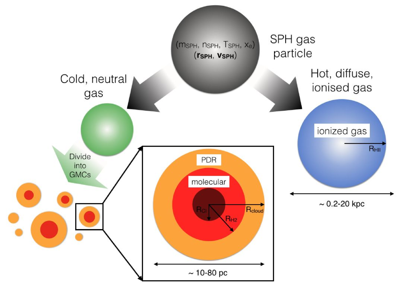
Figure 1.— Schematic illustrating the sub-grid procedures applied to the SPH simulation in post-processing. Each SPH particle is a hybrid of neutral and ionized gas. The neutral gas associated with each SPH gas particle is divided into GMCs with masses and sizes following the Galactic mass-spectrum and mass-size relation for GMCs. Each GMC has an onion-layer structure, set by the stratification of the impinging FUV-field, which consists of outer layer of PDR/atomic gas of Hi and Cii, and an inner molecular region where carbon is found in its single ionized state, and in neutral form further in (Section 4.1). The ionized gas associated with each SPH particle is assumed to reside in spherical clouds with radii and temperatures given by the SPH smoothing length and gas temperature (Section 4.2).

2. Methodology overview

SÍGAME is applied at the post-processing stage of a SPH simulation and takes as its input the following quantities associated with each SPH particle: the position ($[x,y,z]$), velocity ($[v_{x},v_{y},v_{z}]$), smoothing length ($h$), gas mass ($m_{\rm{SPH}}$), hydrogen density ($n_{\rm{H}}$), gas kinetic temperature ($T_{\rm{k}}$), electron fraction ($\mbox{$x_{\rm{e}}$}=n_{e}/n_{\rm H}$), SFR, metallicity ($Z$) as well as the relative abundances of carbon ([C/H]) and oxygen ([O/H]). The key steps involved in the post-processing are illustrated in Fig. 1 and briefly listed below (with details given in subsequent sections):

1. The SPH gas is separated into its neutral and ionized constituents as dictated by the electron fraction provided by the GADGET-3 simulations.

2. The neutral gas is divided into giant molecular clouds (GMCs) according to the observed mass function of GMCs in the Milky Way (MW) and nearby quiescent galaxies. The GMCs are modeled as logotropic spheres with their sizes and internal velocity dispersions derived according to pressure-normalized scaling relations.

3. Each GMC is assumed to consist of three spherically symmetric regions: (1) a FUV-shielded molecular core region where all carbon is locked up in Ci and CO; (2) an outer molecular region where both Ci and Cii can exist; and (3) a largely neutral atomic layer of Hi, Hii and Cii. The last region mimics the FUV-stratified PDRs observed at the surfaces of molecular clouds (Hollenbach & Tielens, 1999). This layer can contain both atomic and ionized gas, but we shall refer to it simply as the PDR gas. The relative extent of these regions within each cloud, and thus the densities at which they occur, ultimately depends on the strength of the impinging FUV-field and CR ionization rate. The latter are set to scale with the local SFR volume density and, by requiring thermal balance with the cooling from line emission (from Cii, Oi, and H₂), determine the temperatures of the molecular and atomic gas phases.

4. The remaining ionized gas of the SPH simulation is divided into Hii clouds of radius equal to the smoothing lengths, temperature equal to that of the SPH simulation and constant density.

5. The [Cii] emission from the molecular, PDR, and diffuse ionized gas is calculated separately and summed to arrive at the total [Cii] emission from the galaxy. In doing so it is assumed that there is no radiative coupling between the clouds in the galaxy.

The SPH simulations used in this paper, and the galaxies extracted from them, are described in the following section.

Table 1Global properties of the seven simulated galaxies used for this work at $z=2$.

	G1	G2	G3	G4	G5	G6	G7
$M_{\rm{\ast}}$ [1010 $\rm{M}_{\odot}$ ]	0.36	0.78	0.95	1.80	4.03	5.52	6.57
$M_{\rm{gas}}$ [1010 $\rm{M}_{\odot}$ ]	0.42	0.68	1.26	1.43	2.59	2.16	1.75
$M_{\rm{neutral}}$ [1010 $\rm{M}_{\odot}$ ]	0.09	0.13	0.57	0.20	0.29	0.29	0.39
$M_{\rm ionized}$ [1010 $\rm{M}_{\odot}$ ]	0.33	0.55	0.69	1.23	1.30	1.87	1.36
SFR [$\rm{M}_{\odot}$ yr-1 ]	4.9	10.0	8.8	25.1	19.9	59.0	37.5
$\Sigma_{\rm{SFR}}$ [$\rm{M}_{\odot}$ yr-1 kpc-2]	0.016	0.032	0.028	0.080	0.063	0.188	0.119
$Z^{\prime}$	0.43	0.85	0.64	1.00	1.00	1.67	1.72

All quantities have been calculated at $z=2$ using a fixed cut-out radius of $R_{\rm cut}=10\,{\rm kpc}$, which is the radius at which the accumulative stellar mass function of each galaxy flattens. $M_{\rm{gas}}$ is the total gas mass, and $M_{\rm{neutral}}$ and $M_{\rm ionized}$ the gas masses in neutral and ionized form, respectively (see Section 4). The metallicity ($\mbox{$Z^{\prime}$}=Z/Z_{\odot}$) is the mean of all SPH gas particles within $R_{\rm cut}$.

3. SPH Simulations

Our simulations are evolved with an updated version of the public GADGET-3 cosmological SPH code (Springel 2005 and S. Huang et al. 2015 in preparation). It includes cooling processes using the primordial abundances as described in Katz et al. (1996), with additional cooling from metal lines assuming photo-ionization equilibrium from Wiersma et al. (2009). We use the more recent ‘pressure-entropy’ formulation of SPH which resolves mixing issues when compared with standard ‘density-entropy’ SPH algorithms (see Saitoh & Makino, 2013; Hopkins, 2013, for further details). Our code additionally implements the time-step limiter of Saitoh & Makino (2009), Durier & Dalla Vecchia (2012) which improves the accuracy of the time integration scheme in situations where there are sudden changes to a particle’s internal energy. To prevent artificial fragmentation (Schaye & Dalla Vecchia, 2008; Robertson & Kravtsov, 2008), we prohibit gas particles from cooling below their effective Jeans temperature which ensures that we are always resolving at least one Jeans mass within a particle’s smoothing length. This is very similar to adding pressure to the ISM as in Springel & Hernquist (2003), Schaye & Dalla Vecchia (2008), except instead of directly pressurizing the gas we prevent it from cooling and fragmenting below the Jeans scale.

We stochastically form stars within the simulation from molecular gas following a Schmidt (1959) law with an efficiency of 1% per local free-fall time (Krumholz & Tan, 2007; Lada et al., 2010). The molecular content of each gas particle is calculated via the equilibrium analytic model of Krumholz et al. (2008, 2009); McKee & Krumholz (2010). This model allows us to regulate star formation by the local abundance of H₂ rather than the total gas density, which confines star formation to the densest peaks of the ISM. Further implementation details can be found in Thompson et al. (2014). Galactic outflows are implemented using the hybrid energy/momentum-driven wind (ezw) model fully described in Davé et al. (2013); Ford et al. (2015). We also account for metal enrichment from Type II supernovae (SNe), Type Ia SNe, and AGB stars as described in Oppenheimer & Davé (2008).

3.1. SPH simulations of $z=2$ MS galaxies

We use the cosmological zoom-in simulations presented in Thompson et al. (2015), and briefly summarized here. Initial conditions were generated using the MUSIC code (Hahn & Abel, 2011) assuming cosmological parameters consistent with constraints from the Planck (Planck Collaboration et al., 2014) results, namely $\Omega_{m}=0.3,\Omega_{\Lambda}=0.7,H_{0}=70,\sigma_{8}=0.8,n_{s}=0.96$. Six target halos were selected at $z=2$ from a low-resolution $N$-body simulation consisting of $256^{3}$ dark-matter particles in a $(16h^{-1}{\rm Mpc})^{3}$ volume with an effective co-moving spatial resolution of $\epsilon=1.25\,h^{-1}$ kpc. Each target halo is populated with higher resolution particles at $z=249$, with the size of each high resolution region chosen to be $2.5$ times the maximum radius of the original low-resolution halo. The majority of halos in our sample are initialized with a single additional level of refinement ($\epsilon=0.625\,h^{-1}$kpc), while the two smallest halos are initialized with two additional levels of refinement ($\epsilon=0.3125\,h^{-1}$kpc).

The six halos produce seven star-forming galaxies at $z=2$ that are free from all low-resolution particles within the virial radius of their parent halo. Their stellar masses ($M_{\rm{\ast}}$) range from $3.6\times 10^{9}$ to $6.6\times 10^{10}\,\mbox{$\rm{M}_{\odot}$}$ and their SFRs from $5$ to $60$ $\rm{M}_{\odot}$ yr^-1 (Table 1). We hereafter label the galaxies G1, …, G7 in order of increasing $M_{\rm{\ast}}$. Other relevant global properties directly inferred from the SPH simulations, such as total gas mass ($M_{\rm{gas}}$), neutral and ionized gas masses ($M_{\rm{neutral}}$ and $M_{\rm ionized}$, respectively), average SFR surface density ($\Sigma_{\rm SFR}$), and average metallicity ($Z^{\prime}$), can also be found in Table 1.

Figure 2.— The SFR–M_∗ relation at $z\simeq 2$ as determined by Speagle et al. (2014) (dashed line) with the location of our seven simulated galaxies highlighted (filled circles). Dotted-dashed and dotted lines indicate the $1\sigma$ and $3\sigma$ scatter around the relation of Speagle et al. (2014). For comparison we also show the locus defined by $3754$ $1.4<z<2.5$ galaxies from the NEWFIRM Medium-Band Survey (gray filled contours), with masses and SFRs calculated using a Kroupa IMF (Whitaker et al., 2011).

Fig. 2 shows the locations of G1, …, G7 in the SFR$-$$M_{\rm{\ast}}$ diagram. The galaxies are consistent with observational determinations of the $z\sim 2$ MS of star-forming galaxies (Whitaker et al., 2011; Speagle et al., 2014).

4. Modeling the ISM

As illustrated in Fig. 1, the first step in modeling the ISM is to split each SPH particle into an ionized and a neutral gas component. This is done using the electron fraction, $x_{\rm{e}}$, associated with each SPH particle, i.e.,:

$$m_{\rm neutral} =(1-\mbox{$x_{\rm{e}}$})\mbox{$m_{\rm{SPH}}$}$$ (1)

$$m_{\rm ionized} =\mbox{$x_{\rm{e}}$}\mbox{$m_{\rm{SPH}}$}.$$ (2)

The electron fraction from GADGET-3 gives the density of electrons relative to that of hydrogen, $\mbox{$n_{\rm{e}}$}/\mbox{$n_{\rm{H}}$}$, and can therefore reach values of $\sim 1.16$ in the case where helium is also ionized. As a result we re-normalized the distribution of $x_{\rm{e}}$ values to a maximal $x_{\rm{e}}$ of 1 so as to not exceed the total gas mass in the simulation. Fig. 3 shows the distribution of SPH gas particles masses in G4 – chosen for its position near the center of the stellar and gas mass ranges of G1, …, G7 – along with the mass distributions of the neutral and ionized gas components obtained from eqs. 1 and 2. The ionized gas is seen to have a relatively flat distribution spanning the mass range $\sim 10^{4.3}-10^{5.8}\,\mbox{$\rm{M}_{\odot}$}$. The neutral gas, however, peaks at two characteristic masses ($\sim 10^{5.5}\,\mbox{$\rm{M}_{\odot}$}$ and $\sim 10^{5.8}\,\mbox{$\rm{M}_{\odot}$}$), where the lower mass peak represents gas particles left over from the first generation of stars in the simulation.

Figure 3.— The distribution of SPH gas particle masses (solid histogram) in G4. The distribution peaks at two characteristic masses ($\sim 10^{5.5}\,\mbox{$\rm{M}_{\odot}$}$ and $\sim 10^{5.8}\,\mbox{$\rm{M}_{\odot}$}$), where the lower mass peak represents gas particles left over from the first generation of stars in the simulation. Splitting the gas into its neutral and ionized components according to eqs. 1 and 2 results in the mass distribution given by the dotted and dashed histograms, respectively.

4.1. GMCs

4.1.1 Masses, sizes and velocity dispersion

The neutral gas mass, $m_{\rm{neutral}}$, associated with a given SPH particle is divided into GMCs by randomly sampling the GMC mass spectrum as observed in the Galactic disk and Local Group galaxies: $\frac{dN}{dm_{\rm GMC}}\propto m_{\rm GMC}^{-\beta}$ with $\beta=1.8$ (Blitz et al., 2007). Similar to Narayanan et al. (2008a, b), a lower and upper cut in mass of $10^{4}\,\mbox{$\rm{M}_{\odot}$}$ and $10^{6}\,\mbox{$\rm{M}_{\odot}$}$, respectively, are enforced in order to ensure the GMC masses stay within the range observed by Blitz et al. (2007). Up to 40 GMCs are created per SPH particle but typically most ($>90\%$) of the SPH particles are split into four GMCs or less. While $m_{\rm{neutral}}$ never exceeds the upper GMC mass limit ($10^{6}\,\mbox{$\rm{M}_{\odot}$}$), there are instances where $m_{\rm{neutral}}$ is below the lower GMC mass limit ($10^{4}\,\mbox{$\rm{M}_{\odot}$}$). In those cases we simply discard the gas, i.e., remove it from any further sub-grid processing. For the highest resolution simulations in our sample (G1 and G2), the discarded neutral gas amounts to $\sim 6\,\%$ of the total neutral gas mass, and $\mathrel{\raise 1.50696pt\hbox{$\scriptstyle<$}\kern-6.00006pt\lower 1.72218pt\hbox{{$\scriptstyle\sim$}}}0.02\,\%$ in the remaining five galaxies. We shall therefore assume that it does not affect our results significantly.

The GMCs are randomly distributed within $0.2\times$ the smoothing length of the original SPH particle, but with the radial displacement scaling inversely with GMC mass in order to retain the original gas mass distribution as closely as possible. To preserve the overall gas kinematics as best possible, all GMCs associated with a given SPH particle are given the same velocity as that of the SPH particle.

GMC sizes are obtained from the pressure-normalized scaling relations for virialized molecular clouds which relate cloud radius ($R_{\rm{GMC}}$) with mass ($m_{\rm GMC}$) and external pressure ($P_{\rm{ext}}$):

$$\frac{\mbox{$R_{\rm{GMC}}$}}{\text{pc}}=\left(\frac{\mbox{$P_{\rm{ext}}$}/k_{\text{B}}}{10^{4}\,\mbox{cm${}^{-3}$}\,\text{K}}\right)^{-1/4}\left(\frac{\mbox{$m_{\rm{GMC}}$}}{290\,\text{\mbox{$\rm{M}_{\odot}$}}}\right)^{1/2}.$$ (3)

We assume $\mbox{$P_{\rm{ext}}$}=P_{\rm tot}/(1+\alpha_{0}+\beta_{0})$ for relative cosmic and magnetic pressure contributions of $\alpha_{0}=0.4$ and $\beta_{0}=0.25$ (Elmegreen, 1989). For the total pressure ($P_{\rm tot}$) we adopt the external hydrostatic pressure at mid-plane for a rotating disk of gas and stars, i.e.,:

$$P_{\rm tot}\approx\frac{\pi}{2}\rm{G}\mbox{$\Sigma_{\rm{gas}}$}\left[\mbox{$\Sigma_{\rm{gas}}$}+\left(\frac{\sigma_{\rm gas,\perp}}{\sigma_{\rm*,\perp}}\right)\mbox{$\Sigma_{\rm{*}}$}\right],$$ (4)

where $\Sigma_{\rm{gas}}$ and $\Sigma_{\rm{*}}$ are the local surface densities of gas and stars, respectively, and $\sigma_{\rm gas,\perp}$ and $\sigma_{\rm*,\perp}$ their local velocity dispersions measured perpendicular to the mid-plane (see e.g., Elmegreen (1989); Swinbank et al. (2011)). For each SPH particle, all of these quantities are calculated directly from the simulation output (using a radius of $R=1$ kpc from each SPH particle), and it is assumed that the resulting $P_{\rm{ext}}$ is the external pressure experienced by all of the GMCs generated by the SPH particle. We find that GMCs in our simulated galaxies are subjected to a wide range of external pressures ($\mbox{$P_{\rm{ext}}$}/k_{\rm B}\sim 10^{2}-10^{7}\,{\rm cm^{-3}\,K}$). For comparison, the range of pressures experienced by clouds in our Galaxy and in Local Group galaxies is $\mbox{$P_{\rm{ext}}$}/k_{\rm B}\sim 10^{3}-10^{7}\,{\rm cm^{-3}\,K}$ with an average of $P_{\rm ext}/k_{\rm B}\sim 10^{4}$ cm^-3  K in Galactic clouds (Elmegreen, 1989; Blitz et al., 2007). This results in GMC sizes in our simulations ranging from $\mbox{$R_{\rm{GMC}}$}=1-300\,{\rm pc}$.

The internal velocity dispersion ($\sigma_{v}$) of the GMCs is inferred from the virial theorem, which provides us with a pressure-normalized $\mbox{$\sigma_{v}$}-R_{\rm GMC}$ relation:

$$\sigma_{v}=1.2\,\mbox{km\,s${}^{-1}$}\left(\frac{\mbox{$P_{\rm{ext}}$}/k_{\rm B}}{10^{4}\,\mbox{cm${}^{-3}$}\,{\rm K}}\right)^{1/4}\left(\frac{\mbox{$R_{\rm{GMC}}$}}{{\rm pc}}\right)^{1/2},$$ (5)

where the normalization of $1.2\,{\rm km\,s^{-1}}$ comes from studies of Galactic GMCs (Larson, 1981; Elmegreen, 1989; Swinbank et al., 2011).

4.1.2 GMC density and temperature structure

We assume a truncated logotropic profile for the total hydrogen number density of the GMCs, i.e.,:

$$\mbox{$n_{\rm{H}}$}(R)=\mbox{$n_{\rm{H,ext}}$}\left(\frac{\mbox{$R_{\rm{GMC}}$}}{R}\right),$$ (6)

where $\mbox{$n_{\rm{H}}$}(R>\mbox{$R_{\rm{GMC}}$})=0$. For such a density profile it can be shown that the external density, $n_{\rm{H,ext}}$, is 2/3 of the average density:

$$\mbox{$n_{\rm{H,ext}}$}=2/3\mbox{$\langle n_{\rm H}\rangle$}=2/3\frac{\mbox{$m_{\rm{GMC}}$}}{4/3\pi\mbox{$m_{\rm{H}}$}\mbox{$R_{\rm{GMC}}$}^{3}}.$$ (7)

While the total hydrogen density follows a logotropic profile, the transition from H₂$\longrightarrow$Hi/Hii is assumed to be sharp. Similarly for the transition from Ci$\longrightarrow$Cii. This is illustrated in Fig. 4, which shows an example density profile of a GMC from our simulations. From the center of the GMC and out to $R_{\rm{H}_{2}}$, hydrogen is in molecular form. Beyond $R_{\rm{H}_{2}}$, hydrogen is found as Hi and Hii out to $R_{\rm{GMC}}$.

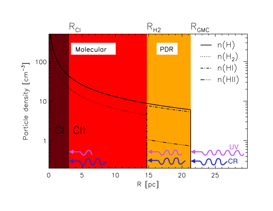
Figure 4.— Example H number density profile (solid line) for a GMC of mass $m_{\rm GMC}=1.3\times 10^{4}$ $\rm{M}_{\odot}$ and radius $R_{\rm GMC}=21$ pc. Also shown are the density profiles of H₂ ($=0.5n_{\rm H}$), Hi and Hii. Note, the transition from molecular to atomic H is assumed to happen instantaneously at $R_{\rm H_{2}}$. The total C abundance follows that of H but scaled with the [C/H] abundance (as provided by the ‘parent’ SPH particle, see Section 2). Cii can exist throughout the cloud except for the very inner region ($R<R_{\rm CI}$; indicated in brown), with the Ci to Cii transition happening instantaneously at $R_{\rm CI}$. [Cii] emission from the layer $R_{\rm CI}\leq R\leq R_{\rm H_{2}}$ (indicated in red) is referred to as ‘molecular’ emission, while [Cii] emission from $R_{\rm H_{2}}<R\leq R_{\rm GMC}$ (indicated in orange) is referred to as ‘PDR’ emission. The relative thickness of these layers is set by the impinging FUV radiation field and cosmic rays (illustrated as purple and blue arrows, respectively), with the former undergoing attenuation further into the cloud.

The size of the molecular region, when adopting the logotropic density profile, is related to the total molecular gas mass fraction ($f^{\prime}_{\rm{mol}}$) of each GMC:

$$f^{\prime}_{\rm{mol}} =\frac{\mbox{$m_{\rm{mol}}$}}{\mbox{$m_{\rm{GMC}}$}}=\frac{\int_{0}^{R_{\rm H_{2}}}\rho_{\rm ext}\frac{R_{\rm GMC}}{R}4\pi R^{2}dR}{\int_{0}^{R_{\rm GMC}}\rho_{\rm ext}\frac{R_{\rm GMC}}{R}4\pi R^{2}dR}$$ (8)

$$=\frac{\int_{0}^{R_{\rm H_{2}}}R\,dR}{\int_{0}^{R_{\rm GMC}}R\,dR}=\left(\frac{R_{\rm H_{2}}}{R_{\rm GMC}}\right)^{2}$$ (9)

$$\Rightarrow\mbox{$r_{\rm{H}_{2}}$}=\sqrt{\mbox{$f^{\prime}_{\rm{mol}}$}},$$ (10)

where $r_{\rm{H}_{2}}$ is the fractional radius, $\mbox{$r_{\rm{H}_{2}}$}=\mbox{$R_{\rm{H}_{2}}$}/\mbox{$R_{\rm{GMC}}$}$. We find $f^{\prime}_{\rm{mol}}$ by assuming $\mbox{\rm{H}{i}}\leftrightarrow\mbox{{\sc H}${}_{2}$}$ equilibrium and using the analytical steady-state approach of Pelupessy et al. (2006) for inferring $f^{\prime}_{\rm{mol}}$ for a logotropic cloud subjected to a radially incident FUV radiation field (see also Olsen et al., 2015). In this framework, the value of $f^{\prime}_{\rm{mol}}$ (and thereby $r_{\rm{H}_{2}}$) depends on:

1. The cloud boundary pressure ($P_{\rm{ext}}$), which is calculated as explained in Section 4.1.1.

2. The metallicity ($Z^{\prime}$) of the GMC, which is inherited from its parent SPH particle and assumed constant throughout the cloud.

3. The kinetic temperature of the gas at the GMC surface ($T_{k}(R_{\rm GMC})$). This quantity is calculated in an iterative process together with $f^{\prime}_{\rm{mol}}$ by solving the following thermal balance equation:

   $$\mbox{$\Gamma_{\rm{PE}}$}+\mbox{$\Gamma_{\rm{CR,H}\textsc{i}}$}=\mbox{$\Lambda_{\rm{C}\rm{\textsc{ii}}}$}+\mbox{$\Lambda_{\rm{O}\rm{\textsc{i}}}$},$$ (11)

   where $\Gamma_{\rm{PE}}$ is the heating rate associated with the photoelectric ejection of electrons from dust grains by the FUV field and $\Gamma_{\rm{CR,H}\textsc{i}}$ is the heating rate by cosmic rays in atomic gas. The main cooling agents are assumed to be due to [Cii] and [Oi]($63\,{\rm\mu m}$ and $145\,{\rm\mu m}$) line emission (i.e., $\Lambda_{\rm{C}\rm{\textsc{ii}}}$ and $\Lambda_{\rm{O}\rm{\textsc{i}}}$, respectively). $\Gamma_{\rm{PE}}$, $\Gamma_{\rm{CR,H}\textsc{i}}$, and $\Lambda_{\rm{C}\rm{\textsc{ii}}}$ all depend on the electron fraction at $R_{\rm GMC}$, which is determined by the degree of Hi ionization by the local FUV radiation field and CR ionization rate (see below for how these quantities are derived). For analytical expressions for the heating rates, we refer to Olsen et al. (2015). For $\Lambda_{\rm O\textsc{i}}$ we use the expressions given in Röllig et al. (2006). The calculation of $\Lambda_{\rm{C}\rm{\textsc{ii}}}$ at the GMC surface is detailed in Section 5 and Appendix A.

4. The strength of the local FUV radiation field ($G_{0}$) and the CR ionization rate ($\zeta_{\rm{CR}}$) impinging on the GMCs. These quantities do not come out from the simulation directly, and instead they are calculated by scaling the Galactic FUV field ($G_{\rm 0,MW}$) and CR ionization rate ($\zeta_{\rm CR,MW}$) with the local SFR volume density in the simulations, i.e., $G_{\rm 0}\propto G_{\rm 0,MW}\left({\rm SFRD}_{\rm local}/{\rm SFRD}_{\rm MW}\right)$ and $\zeta_{\rm CR}\propto\zeta_{\rm CR,MW}\left({\rm SFRD}_{\rm local}/{\rm SFRD}_{\rm MW}\right)$, where ${\rm SFRD_{\rm local}}$ is estimated for each SPH particle as the volume averaged SFR within a $2\,{\rm kpc}$ radius. We have adopted Milky Way values of $G_{\rm 0,MW}=0.6\,{\rm Habing}$ (Seon et al., 2011) and $\zeta_{\rm CR,MW}=3\times 10^{-17}\,{\rm s^{-1}}$ (Webber, 1998). For ${\rm SFRD}_{\rm MW}$ we adopt $0.0024\,{\rm\mbox{$\rm{M}_{\odot}$}\,yr^{-1}\,kpc^{-3}}$, inferred from the average Galactic SFR ($0.3\,{\rm\mbox{$\rm{M}_{\odot}$}\,yr^{-1}}$) within a disk $10\,{\rm kpc}$ in radius and $0.2\,{\rm kpc}$ in height (Heiderman et al., 2010; Bovy et al., 2012).

5. The electron fraction at the cloud boundary. This fraction is not the previously introduced $x_{\rm{e}}$, which was inherent to the SPH simulations and used to split the SPH gas into a neutral and ionized gas phase. Instead, it is the electron fraction given by the degree of ionization of Hi caused by the $G_{0}$ and $\zeta_{\rm{CR}}$ impinging on the cloud. This fraction (and thus the Hi:Hii ratio) is calculated with CLOUDY v13.03 (Ferland et al., 2013) given the hydrogen density and temperature at the cloud boundary and assuming an unattenuated $G_{0}$ and $\zeta_{\rm{CR}}$ at $R_{\rm GMC}$.

The [Cii] emitting region in each of our GMCs is defined as the layer between the surface of the cloud and the depth at which the abundances of C and C⁺ are equal. Hence, if the latter occurs at a radius $R_{\rm{C}\textsc{i}}$ from the cloud center, the thickness of the layer is $\mbox{$R_{\rm{GMC}}$}-\mbox{$R_{\rm{C}\textsc{i}}$}$ (Fig. 4). At radii $<\mbox{$R_{\rm{C}\textsc{i}}$}$, all carbon atoms are for simplicity assumed to be in neutral form. In order to determine the fractional radius $r_{\rm{{\sc C\textsc{i}}}}$ ($=R_{\rm CI}/R_{\rm GMC}$) we follow the work of Röllig et al. (2006) (but see also Pelupessy & Papadopoulos, 2009), who considers the following dominant reaction channels for the formation and destruction of C⁺:

$$\rm{C}+\gamma \rightarrow\rm{C}^{+}+{\it e^{-}}$$ (12)

$$\rm{C}^{+}+{\it e^{-}} \rightarrow\rm{C}+\gamma$$ (13)

$$\rm{C}^{+}+\rm{H}_{2} \rightarrow\rm{CH}^{+}_{2}+\gamma.$$ (14)

In this case, $r_{\rm{{\sc C\textsc{i}}}}$ can be found by solving the following equation:

$$5.13\times 10^{-10} {\rm s^{-1}}\mbox{$G_{0}$}\int_{1}^{\infty}\frac{e^{-\mu\xi_{\rm FUV}A_{\rm V}(\mbox{$r_{\rm{{\sc C\textsc{i}}}}$})}}{\mu^{2}}d\mu$$ (15)

$$= ~{}n_{\rm H}(r_{\rm C{\textsc{i}}})[a_{\rm C}\mbox{$X_{\rm{C}}$}+0.5k_{\rm C}],$$

where the left-hand side is the C⁺ formation rate due to photo-ionization by the attenuated FUV field at $r_{\rm{{\sc C\textsc{i}}}}$ (eq. 12), and the right-hand side is the destruction rate of C⁺ due to recombination and radiative association (eqs. 13 and 14). The constants $a_{\rm C}=3\times 10^{-11}$ cm^-3 s^-1 and $k_{\rm C}=8\times 10^{-16}$ cm^-3 s^-1 are the recombination and radiative association rate coefficients. Note, we have accounted for an isotropic FUV field since $\mu=\cos\theta$, where $\theta$ is the angle between the Poynting vector and the normal direction. $A_{\rm V}(\mbox{$r_{\rm{{\sc C\textsc{i}}}}$})$ is the visual extinction corresponding to the $\mbox{$R_{\rm{GMC}}$}-\mbox{$R_{\rm{C}\textsc{i}}$}$ layer, and is given by $A_{\rm V}(\mbox{$r_{\rm{{\sc C\textsc{i}}}}$})=0.724\sigma_{\rm dust}\mbox{$Z^{\prime}$}\langle n_{\rm H}\rangle\mbox{$R_{\rm{GMC}}$}\ln\left(\mbox{$r_{\rm{{\sc C\textsc{i}}}}$}^{-1}\right)$, where $\sigma_{\rm dust}=4.9\times 10^{-22}\,\mbox{cm${}^{2}$}$ is the FUV dust absorption cross section (Pelupessy & Papadopoulos, 2009; Mezger et al., 1982). $\xi_{\rm FUV}$ accounts for the difference in opacity between visual and FUV light and is set to $3.02$. $X_{\rm{C}}$ is the carbon abundance relative to H and is calculated by adopting the carbon mass fractions of the parent SPH particle (self-consistently calculated as part of the overall SPH simulation) and assuming it to be constant throughout the GMC.

Figure 5.— Top: the number distribution of GMC masses (solid histogram) together with the number distributions of the molecular (dashed histogram) and PDR (dotted histogram) gas component. Middle: GMC-mass-weighted distributions of $R_{\rm{C}\textsc{i}}$ (dotted), $R_{\rm{H}_{2}}$ (dashed) and $R_{\rm{GMC}}$ for GMCs in G4. Bottom: GMC-mass-weighted distributions of the temperature at $R_{\rm{H}_{2}}$ (dashed) and at the cloud surfaces (solid) for GMCs in G4.

The temperature of the [Cii]-emitting molecular gas (i.e., from the gas layer between $R_{\rm{C}\textsc{i}}$ and $R_{\rm{H}_{2}}$) is assumed to be constant and equal to the temperature at $R_{\rm{H}_{2}}$. The latter is given by the thermal balance:

$$\mbox{$\Gamma_{\rm{PE}}$}+\mbox{$\Gamma_{\rm{CR,H}_{2}}$}=\mbox{$\Lambda_{\rm{H}_{2}}$}+\mbox{$\Lambda_{\rm{C}\rm{\textsc{ii}}}$}+\mbox{$\Lambda_{\rm{O}\rm{\textsc{i}}}$},$$ (16)

where $\Gamma_{\rm{CR,H}_{2}}$  is the CR heating in molecular gas, and $\Lambda_{\rm{H}_{2}}$ is the cooling due to the S(0) and S(1) rotational lines of H₂ (Papadopoulos et al. (2014); see also Olsen et al. 2015). $\Gamma_{\rm{CR,H}_{2}}$ depends on $x_{\rm{e}}$, which is calculated with CLOUDY for the local CR ionization rate and the attenuated FUV field at $r_{\rm{H}_{2}}$, i.e. $\mbox{$G_{0}$}e^{-\xi_{\rm FUV}A_{\rm V}(\mbox{$r_{\rm{H}_{2}}$})}$. $A_{\rm V}(\mbox{$r_{\rm{H}_{2}}$})$ corresponds the extinction through the outer atomic transition layer of each GMC.

The temperature of the PDR gas (i.e., from the gas between $R_{\rm{H}_{2}}$ and $R_{\rm{GMC}}$) is assumed to be constant and equal to the temperature at $R_{\rm{GMC}}$.

For each GMC we solve in an iterative manner simultaneously for $R_{\rm{H}_{2}}$ (eq. 10) and $R_{\rm{C}\textsc{i}}$ (eq. 15), as well as for the gas temperature at $R_{\rm{GMC}}$ and at $R_{\rm{H}_{2}}$ (eqs. 11 and 16, respectively)

The resulting distributions of $R_{\rm{H}_{2}}$ and $R_{\rm{C}\textsc{i}}$ for the GMC population in G4 are shown in Fig. 5 (middle panel), along with the distribution of $R_{\rm GMC}$ (obtained from eq. 3). In GMCs in general, we expect $R_{\rm C\textsc{i}}<R_{\rm H_{2}}$, due to efficient H₂ selfshielding. However, as Fig. 5 shows some of the GMCs in our simulations have very small $R_{\rm{H}_{2}}$ (due to them having virtually zero molecular gas fractions), and in those cases $R_{\rm{C}\textsc{i}}$ can be equal to or even exceed $R_{\rm{H}_{2}}$. The latter implies that the [Cii] emission is only coming from the PDR phase, with no contribution from the molecular gas.

The distributions of the kinetic temperature of the gas at $R_{\rm{H}_{2}}$ and $R_{\rm{GMC}}$ for the GMC population in G4 are also shown in Fig. 5 (bottom panel). The temperatures at the cloud surfaces range from $\sim 8\,{\rm K}$ to $\sim 10^{5.5}\,{\rm K}$, and the temperatures at $R_{\rm{H}_{2}}$ lies between $\sim 8$ and $1800\,{\rm K}$.

With $R_{\rm{H}_{2}}$ and $R_{\rm{C}\textsc{i}}$ determined for each GMC we can calculate the gas masses associated with the molecular and PDR gas phase, respectively. The resulting mass distributions are shown in the top panel of Fig. 5, along with the distribution of total GMC masses ($m_{\rm GMC}$) as determined by the adopted GMC mass spectrum (Section 4.1.1). We see that most of the molecular and PDR gas masses follow the total GMC mass spectrum. There is, however, a fraction of GMCs with extremely small molecular gas masses (corresponding to $\mbox{$f^{\prime}_{\rm{mol}}$}\sim 0$). On the other hand, there are some GMCs with small PDR gas masses, i.e., clouds that are so shielded from FUV radiation that they are almost entirely molecular.

4.2. The ionized gas

The ionized gas in our simulations (see eq. 2), is assumed to be distributed in spherical clouds of uniform densities and with radii ($R_{\rm H\textsc{ii}}$) equal to the smoothing lengths of the original SPH particles. These ionized regions in our simulations are furthermore assumed to be isothermal with the temperatures equal to that of the SPH gas. Fig. 6 shows the size (top) and temperature (bottom) distribution for the ionized clouds in G4. Cloud sizes range from $\sim 0.1$ to $\sim 10\,{\rm kpc}$, with more than $60\,\%$ of the ionized gas mass residing in clouds of size $\mathrel{\raise 1.50696pt\hbox{$\scriptstyle<$}\kern-6.00006pt\lower 1.72218pt\hbox{{$\scriptstyle\sim$}}}1000\,{\rm pc}$. For comparison, the range of observed sizes of Hii clouds in nearby galaxies is $10-1000\,{\rm pc}$ (Oey & Clarke, 1997; Hodge et al., 1999). The temperatures range from $\sim 10^{2}\,{\rm K}$ to $\sim 10^{6}\,{\rm K}$ with the bulk of the ionized gas having temperatures $\sim 10^{4-5}\,{\rm K}$.

Figure 6.— Mass-weighted histograms of the size (top) and temperature (bottom) distributions of the ionized clouds in G4.

5. The [Cii] line emission

The [Cii] luminosity of a region of gas is the volume-integral of the effective [Cii]  cooling rate per volume, i.e.,:

$$\mbox{$L_{\rm{[C}\rm{\textsc{ii}]}}$}=\int_{\rm\Delta V}\mbox{$\Lambda_{\rm{C}\rm{\textsc{ii}}}$}\,dV.$$ (17)

Since we have adopted spherical symmetry in our sub-grid treatment of the clouds (both neutral and ionized), we have:

$$L_{\rm{[C}\rm{\textsc{ii}]}} =4\pi\int_{R_{1}}^{R_{2}}\mbox{$\Lambda_{\rm{C}\rm{\textsc{ii}}}$}R^{2}dR,$$ (18)

where $R_{1}=R_{\rm C\textsc{i}}$ and $R_{2}=R_{\rm H_{2}}$ for the molecular phase; $R_{1}=R_{\rm H_{2}}$ and $R_{2}=R_{\rm GMC}$ for the PDR region, and $R_{1}=0$ and $R_{2}=R_{\rm H\textsc{ii}}$ for the ionized gas.

The effective [Cii] cooling rate is:

$$\mbox{$\Lambda_{\rm{C}\rm{\textsc{ii}}}$}=A_{\rm ul}\beta f_{\rm u}\mbox{$n_{\rm{C}\textsc{ii}}$}h\nu,$$ (19)

where $A_{\rm ul}$ ($=$2.3$\times 10^{-6}$ s^-1) is the Einstein coefficient for spontaneous decay. We ignore the effects of any background radiation field from dust and the cosmic microwave background (CMB). $\beta$ is the [Cii] photon escape probability for a spherical geometry (i.e., $\beta=(1-exp(-\tau))/\tau$, where $\tau$ is the [Cii] optical depth). $f_{u}$ is the fraction of singly ionized carbon in the upper ${}^{2}P_{3/2}$ level and is determined by radiative processes and collisional (de)excitation (see Appendix A). The latter can occur via collisions with $e^{-}$, Hi, or H₂, depending on the state of the gas. In our simulations the collisional partner is H₂ in the molecular phase, Hi and $e^{-}$ in the PDR regions, and $e^{-}$ in the ionized gas. Analytical expressions for the corresponding collision rate coefficients as a function of temperature are given in Appendix A. $n_{\rm{C}\textsc{ii}}$ is the number density of singly ionized carbon and is given by $\mbox{$n_{\rm{C}\textsc{ii}}$}=X_{\rm C}f_{\rm C\textsc{ii}}n_{\rm H}$, where $f_{\rm C\textsc{ii}}$ is the fraction of carbon atoms in the singly ionized state. For the latter we used tabulated fractions from CLOUDY v13.03 over a wide range in temperature, hydrogen density, FUV field strength, and CR ionization rate.

We calculate the integral in eq. 18 numerically by splitting the $R_{2}-R_{1}$ region up into 100 radial bins. In each bin, $n_{\rm H}$ is set to be constant and – in the case of the molecular and PDR regions – given by the logotropic density profile at the radius of the given bin (Fig. 4). For the ionized clouds, $n_{\rm H}$ is constant throughout (Section 4.2). For the PDR regions (i.e., from $R_{\rm H_{2}}$ to $R_{\rm GMC}$) we assume that the temperature, electron fraction and $G_{0}$ are kept fixed to the outer boundary value at $R_{\rm GMC}$ (i.e., no attenuation of the FUV field). This implies that the [Cii] luminosity from the PDR gas is an upper limit. Similar for the [Cii] emission from the molecular region (i.e., from $R_{\rm C\textsc{i}}$ to $R_{\rm H_{2}}$), where we assume that the temperature throughout this region is fixed to its values at $R_{\rm H_{2}}$. Also, throughout this region we adopt the attenuated FUV field at $R_{\rm H_{2}}$.

6. Results and discussion

Having divided the ISM in our galaxies into molecular, atomic and ionized gas phases, and having devised a methodology for calculating their [Cii] emission, we are now in a position to quantify the relative contributions from the aforementioned gas phases to the total [Cii] emission, and examine their relationship to the on-going star formation.

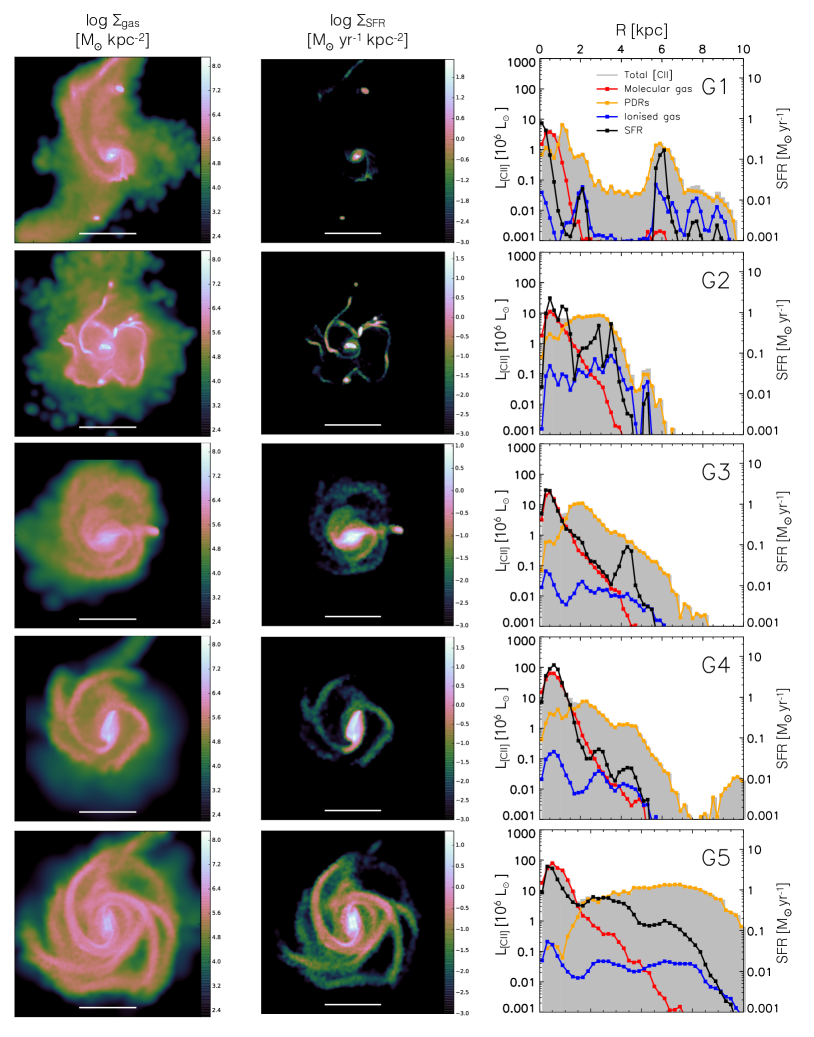
Figure 7.— Gas and SFR surface density maps (left and middle columns, respectively) of our SPH simulated galaxies viewed face-on (G1, …, G7 from top to bottom; see also Thompson et al. (2015)). The horizontal white bars correspond to a physical scale of $5\,{\rm kpc}$. The right-hand column shows the radial profiles of the total [Cii] luminosity (gray histogram) and the contributions from molecular gas (red curve), PDR (orange curve) and ionized gas (blue curve). The SFR radial profiles are also shown (black curve). The radial profiles were determined by summing up the [Cii] luminosity and SFR within concentric rings with fixed width of $0.2\,{\rm kpc}$.

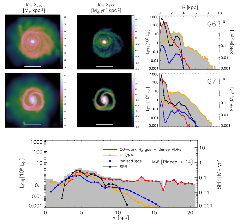
Figure 7.— Continued. In the bottom panel we show for reference the radial $L_{\rm{[C}\rm{\textsc{ii}]}}$ profile of the Galaxy (gray histogram) along with the contributions from CO-dark H₂ gas and dense PDRs (red curve), cold H i (orange curve), and ionized gas (blue curve) (Pineda et al., 2014). Also shown is the radial SFR profile (black curve) inferred from the $1.4\,$GHz intensity distribution. Fixed radial bin widths of $0.5\,{\rm kpc}$ have been adopted (see Pineda et al. (2014) for details).

6.1. Radial [Cii] luminosity profiles

First, however, to get a sense of the distribution of gas and star formation in our simulated galaxies, we show in Fig. 7 surface density maps of the total SPH gas (left column) and star formation rate (middle column) when viewed face-on. The maps reveal spiral galaxy morphologies, albeit with some variety: some (G1, G2 and G3) show perturbed spiral arms due to on-going mergers with satellite galaxies; others (G4, G5, G6 and G7) have seemingly undisturbed, grand-design spiral arms; a central bar-like structure is also seen in some (G2, G4, G5 and G7). Overall, the star formation is seen to be much more centrally concentrated than the SPH gas. This is especially true for G1 and G2, which have very centrally peaked star formation. The radial SFR and [Cii] luminosity profiles of G1, …, G7 – derived by summing up the SFR and the [Cii] luminosity within concentric rings (of fixed width: $0.2\,{\rm kpc}$) – are also shown in Fig. 7. We have inferred the radial [Cii] luminosity distribution for the full ISM as well as for the individual gas phases.

The radial SFR profiles of our model galaxies typically peak at $R\sim 0.5\,{\rm kpc}$ (in G1 at $R\mathrel{\raise 1.50696pt\hbox{$\scriptstyle<$}\kern-6.00006pt\lower 1.72218pt\hbox{{$\scriptstyle\sim$}}}0.5\,{\rm kpc}$) and then tail off with radius. In some cases, local peaks in the star formation activity occur at galactocentric distances $\mathrel{\raise 1.50696pt\hbox{$\scriptstyle>$}\kern-6.00006pt\lower 1.72218pt\hbox{{$\scriptstyle\sim$}}}2\,{\rm kpc}$, corresponding to the locations of either satellite galaxies (G2 and G3) or spiral arms (G5 and G7).

The total [Cii] luminosity profiles (gray histograms) also peak at $R\sim 0.5\,{\rm kpc}$, and within the central $R\mathrel{\raise 1.50696pt\hbox{$\scriptstyle<$}\kern-6.00006pt\lower 1.72218pt\hbox{{$\scriptstyle\sim$}}}1.5\,{\rm kpc}$ there is in general a good correspondence between the total [Cii] emission and the star formation activity. This correspondence is driven by the molecular gas phase which dominates the [Cii] emission in the central regions. The molecular [Cii] emission is seen to correlate strongly with the star formation out to radii $\sim 5\,{\rm kpc}$ and beyond (e.g., G3 and G4). There are cases, however, where localized enhancements in the SFR are not matched by increased [Cii] emission from the molecular gas (e.g. G2, and G3). These SFR enhancements are reflected in the [Cii] emission profile of the ionized gas, which at galactocentric distances $\mathrel{\raise 1.50696pt\hbox{$\scriptstyle>$}\kern-6.00006pt\lower 1.72218pt\hbox{{$\scriptstyle\sim$}}}2\,{\rm kpc}$ follow the SFR closely (despite contributing only a small fraction to the total [Cii] emission budget, see below). In contrast, the [Cii] emission from the PDR gas, which dominates the total [Cii] luminosity at $2.0\,{\rm kpc}\mathrel{\raise 1.50696pt\hbox{$\scriptstyle<$}\kern-6.00006pt\lower 1.72218pt\hbox{{$\scriptstyle\sim$}}}R\mathrel{\raise 1.50696pt\hbox{$\scriptstyle<$}\kern-6.00006pt\lower 1.72218pt\hbox{{$\scriptstyle\sim$}}}10\,{\rm kpc}$, does not appear to be a sensitive tracer of the SFR. At $R\mathrel{\raise 1.50696pt\hbox{$\scriptstyle<$}\kern-6.00006pt\lower 1.72218pt\hbox{{$\scriptstyle\sim$}}}1.5\,{\rm kpc}$ where the SFR peaks, the [Cii] emission from this phase is seen to drop. At larger radii, the PDR [Cii] emission declines but at a more gradual rate than the star formation.

In the bottom right panel of Fig. 7 we show the Galactic SFR and [Cii] luminosity radial profiles from Pineda et al. (2014), who observed the [Cii] emission from (1) CO-dark H₂ gas and dense PDRs, (2) cold neutral Hi gas, and (3) hot ionized gas in our own Galaxy. In order to facilitate an approximate comparison with our simulations we identify these three Galactic ISM phases with the molecular, atomic, and ionized gas in our simulations. It is important to keep in mind, however, that the ISM in our simulations has a higher pressure, is kinematically more violent, and is more actively forming stars than is the case in our Galaxy.

The SFR and [Cii] profiles in our Galaxy peak at larger radii ($R\sim 4-5\,$kpc) than in our simulated galaxies. This is not surprising given the low content of star formation and gas in the Galactic bulge, and the fact that the bulk of star formation in our Galaxy takes place in the disk. In contrast, gas is still being funneled toward the central regions of our simulated galaxies where it is converted into stars. Thus the SFR level in our simulated galaxies is much higher (by $\mathrel{\raise 1.50696pt\hbox{$\scriptstyle>$}\kern-6.00006pt\lower 1.72218pt\hbox{{$\scriptstyle\sim$}}}10\times$) and more centrally concentrated than in our Galaxy, where stars form at a rate of $\mathrel{\raise 1.50696pt\hbox{$\scriptstyle<$}\kern-6.00006pt\lower 1.72218pt\hbox{{$\scriptstyle\sim$}}}0.1-1\,{\rm\mbox{$\rm{M}_{\odot}$}\,yr^{-1}}$ across the disk. Remarkably, significant levels of [Cii] emission extend out to $R\sim 20\,{\rm kpc}$ in our Galaxy, well beyond the point where star formation has ceased. Here, the emission is completely dominated by CO-dark H₂ gas and dense PDR regions. This is similar to the picture seen in our simulated galaxies where the [Cii] emission at large radii is dominated by a neutral gas phase – designated PDR gas in our simulations, dubbed CO-dark H₂ $+$ dense PDR gas in Pineda et al. (2014) – that is largely uncoupled from star formation. The radial [Cii] profile of the ionized gas in the Galaxy roughly follows the SFR profile, as is the case in our simulations.

Fig. 8 displays the fractional [Cii] luminosity from the different ISM phases: top panel for the entire disk ($R<10\,{\rm kpc}$), middle panel for the central region ($R\leq 1\,{\rm kpc}$), and bottom panel for the outer disk ($R>2\,{\rm kpc}$). Within $R\leq 10\,{\rm kpc}$, the molecular gas can constitute from $\sim 31\%$ (G2) to $\sim 91\,\%$ (G7) of the total [Cii] luminosity; for the PDR gas the range is $\sim 9\%$ (G7) to $\sim 67\%$ (G2). Fig. 8 shows that the contribution from the molecular gas to the total [Cii] emission increases with the overall SFR of the galaxy. A reverse trend is seen for the PDR gas. As expected, the total [Cii] emission from the central regions ($R\leq 1\,{\rm kpc}$) is dominated by the molecular gas ($\mathrel{\raise 1.50696pt\hbox{$\scriptstyle>$}\kern-6.00006pt\lower 1.72218pt\hbox{{$\scriptstyle\sim$}}}70\%$) while further our ($R>2\,{\rm kpc}$) the PDR gas phase dominates ($\mathrel{\raise 1.50696pt\hbox{$\scriptstyle>$}\kern-6.00006pt\lower 1.72218pt\hbox{{$\scriptstyle\sim$}}}90\%$) (see Fig. 8, bottom two panels). For reference, we note that in our own Galaxy about $55\,\%$ of the total Galactic [Cii] luminosity (within $R\mathrel{\raise 1.50696pt\hbox{$\scriptstyle<$}\kern-6.00006pt\lower 1.72218pt\hbox{{$\scriptstyle\sim$}}}20\,{\rm kpc}$) is from molecular gas and dense PDRs, $25\,\%$ from cold Hi, and $20\,\%$ from the ionized gas (Pineda et al., 2014). Thus, the ionized phase is a more important contributor to the overall [Cii] budget in our Galaxy than in the simulated galaxies presented here where the contribution from the ionized gas is $\mathrel{\raise 1.50696pt\hbox{$\scriptstyle<$}\kern-6.00006pt\lower 1.72218pt\hbox{{$\scriptstyle\sim$}}}3\%$ in all cases.

6.2. The integrated $\mbox{$L_{\rm{[C}\rm{\textsc{ii}]}}$}-{\rm SFR}$ relation

Fig. 9 shows the integrated ${\rm\mbox{$L_{\rm{[C}\rm{\textsc{ii}]}}$}-SFR}$ relations for our simulated galaxies: top panel for the full ISM and, in separate panels below, for each of the three ISM phases considered in our simulations.

Figure 8.— Contributions to the total [Cii] luminosity from the molecular (red), PDR (yellow), and ionized (blue) gas phases for each of our simulated galaxies, ranked according to their total SFRs. The three panels show the relative contributions within $R<10\,{\rm kpc}$ (top), for $R<1\,{\rm kpc}$ (middle), and for $R>2\,{\rm kpc}$ (bottom). The horizontal dashed lines and the percentages given indicate the relative contributions to the total [Cii] luminosity of our own Galaxy from CO-dark H₂ + dense PDR gas (red; 55%), cold atomic gas (yellow; 25%), and ionized gas (blue; 20%) (Pineda et al., 2014). The total SFR of the Galaxy is $1.9\,{\rm\mbox{$\rm{M}_{\odot}$}\,yr^{-1}}$ (Chomiuk & Povich, 2011).

When considering the entire ISM a tight correlation between $L_{\rm{[C}\rm{\textsc{ii}]}}$ and SFR emerges, which is well fit in log-log space by a straight line with slope $1.27\pm 0.17$ (solid line in the top panel). This relation is largely set by the molecular and PDR gas phases. The molecular gas phase, itself exhibiting a strong correlation between [Cii] and SFR with slope $1.72\pm 0.22$, drives the slope of the total correlation. The PDR gas on the other hand, shows a weaker [Cii] $-$SFR correlation with a slope of $0.43\pm 0.20$ but contributes significantly to the normalization of the total ${\rm\mbox{\rm{[C}{ii}]}-SFR}$ relation, especially at the low SFR end (see Fig. 9). The [Cii] emission from the ionized gas also shows a weak dependency on SFR (slope $0.44\pm 0.30$) but does not contribute significantly to the total [Cii]  emission, its normalization factor being $\mathrel{\raise 1.50696pt\hbox{$\scriptstyle>$}\kern-6.00006pt\lower 1.72218pt\hbox{{$\scriptstyle\sim$}}}10\times$ below that of the molecular and PDR gas (Fig. 9, bottom panel).

Figure 9.— $L_{\rm{[C}\rm{\textsc{ii}]}}$ vs. SFR for our simulated galaxies (big filled circles). The same color-coding as in Fig. 2 is used and listed again for convenience in the bottom panel. From top to bottom panel we show the [Cii] luminosity from the full ISM (gray), the molecular gas (red), PDRs (orange), and ionized gas (blue). For comparison, we show individual [Cii] observations of 54 $z\sim 0$ spirals (purple filled circles; Malhotra et al., 2001), with the best fit to this sample given by the dotted line (see main text for details). Also shown are 240 $z\sim 0$ (U)LIRGs (purple open circles; Díaz-Santos et al., 2013; Farrah et al., 2013), and 12 $z\sim 0.3$ (U)LIRGs (red triangles; Magdis et al., 2014). The high-$z$ comparison samples include 25 $1<z<6$ star-forming galaxies (cyan squares; D14) and the dashed line indicate the best fit to this sample. Also shown are 16 $z\sim 4-7$ quasars (green triangles; Iono et al., 2006; Walter et al., 2009; Wagg et al., 2010; Gallerani et al., 2012; Wang et al., 2013; Venemans et al., 2012; Carilli et al., 2013; Willott et al., 2013), and 10 normal star-forming $z\sim 5-6$ galaxies (magenta stars) observed by Capak et al. (2015). The Galaxy is shown for reference with a gray cross (Pineda et al., 2014).

In the top panel of Fig. 9 we compare the ${\rm\mbox{$L_{\rm{[C}\rm{\textsc{ii}]}}$}-SFR}$ relation obtained from our simulated galaxies with samples of [Cii] detected galaxies in the redshift range $z\sim 0-6.5$ compiled from the literature. Our simulated galaxies are seen to match the observed ${\rm\mbox{$L_{\rm{[C}\rm{\textsc{ii}]}}$}-SFR}$ relation both in terms of the slope of the relation and its overall normalization. A power-law fit to the simulated galaxies (shown as solid line in Fig. 9) yields a near-linear slope ($1.27\pm 0.17$). Normal star-forming galaxies at $z\sim 0$, with similar levels of SFR ($\sim 0.2-100\,{\rm\mbox{$\rm{M}_{\odot}$}\,yr^{-1}}$; Malhotra et al. 2001) as our simulated galaxies, are consistent with a linear correlation given by $L_{\rm[C\,\textsc{ii}]}=1.05\times 10^{7}{\rm SFR}$ (dotted line in Fig. 9) with a scatter of $0.3\,{\rm dex}$ (Magdis et al., 2014). The scatter of our simulated galaxies around their best-fit relation is $0.14\,{\rm dex}$, i.e., significantly lower. We attribute this to the fact that our simulated galaxies constitute a fairly homogeneous (and small) sample spanning a rather small range in SFR, $L_{\rm[C\textsc{ii}]}$, and $Z^{\prime}$, unlike the observed samples with which we are comparing.

A direct comparison with [Cii]-detected galaxies at high redshifts is complicated by the fact that the latter typically have significantly larger SFRs than our model galaxies. Furthermore, high-$z$ samples are often heterogeneous (e.g., significant AGN contribution, cf. Gullberg et al., 2015). One exception, however, is the recent [Cii]-detected sample of star-forming galaxies at $z\simeq 5-6$ presented by Capak et al. (2015) (shown as magenta stars in Fig. 9), which span the same range in SFR as our simulations. These galaxies are seen to be in excellent agreement with the ${\rm\mbox{$L_{\rm{[C}\rm{\textsc{ii}]}}$}-SFR}$ relation defined by our simulations, both in terms of slope and normalization.

Extrapolating our best-fit relation to SFRs $\mathrel{\raise 1.50696pt\hbox{$\scriptstyle>$}\kern-6.00006pt\lower 1.72218pt\hbox{{$\scriptstyle\sim$}}}300\,{\rm\mbox{$\rm{M}_{\odot}$}\,yr^{-1}}$ in order to compare with other high-$z$ samples, the relation is seen to overshoot the data. A power-law fit to the $z>1$ star-forming galaxies with SFR $\gtrsim 300$ $\rm{M}_{\odot}$ yr^-1 compiled by D14 yields: $L_{\rm[C\,\textsc{ii}]}=1.7\times 10^{7}{\rm SFR}^{0.85}$ (D14; shown as the dashed line in Fig. 9), i.e., formally, a shallower relation than that of our simulated galaxies and that of the $z\sim 0$ sample (albeit less so). Finally, we stress that the [Cii]-detected galaxies at $z>1$ with SFRs $\mathrel{\raise 1.50696pt\hbox{$\scriptstyle>$}\kern-6.00006pt\lower 1.72218pt\hbox{{$\scriptstyle\sim$}}}300\,{\rm\mbox{$\rm{M}_{\odot}$}\,yr^{-1}}$ likely derive from rather complex environments (e.g. Narayanan et al., 2015), which may not correspond to the relatively quiescent MS star-forming galaxies modeled here.

6.3. The resolved $\mbox{$\Sigma_{\rm{[C\textsc{ii}]}}$}-\mbox{$\Sigma_{\rm{SFR}}$}$ relation

In Fig. 10 we show the combined ${\rm\mbox{$\Sigma_{\rm{[C\textsc{ii}]}}$}-\mbox{$\Sigma_{\rm{SFR}}$}}$ relation of all seven simulated galaxies in their face-on configuration. The relation is shown for the entire ISM (top panel) and for each of the separate gas phases (bottom three panels). Surface densities were determined within 1 kpc $\times$ 1 kpc regions. Contours reflect the number of regions at a given ($\Sigma_{\rm{SFR}}$,$\Sigma_{\rm{[C\textsc{ii}]}}$)-combination and are given as percentages of the peak number of regions.

Given the variations in the local star formation conditions within our model galaxies, we can explore the relationship between [Cii] and star formation over a much wider range of star formation intensities than is possible with the integrated quantities. A ${\rm\mbox{$\Sigma_{\rm{[C\textsc{ii}]}}$}-\mbox{$\Sigma_{\rm{SFR}}$}}$ correlation spanning more than five decades in $\Sigma_{\rm{SFR}}$ is seen for the entire ISM as well as for the individual ISM phases. Similar to the integrated [Cii] vs. SFR relations in the previous section, the molecular and PDR phases dominate the resolved [Cii] emission budget at all SFR surface densities, and with the molecular relation being steepest and exhibiting the largest degree of scatter. The resolved [Cii] emission from the ionized phase, while clearly correlated with $\Sigma_{\rm{SFR}}$, is largely negligible at all star formation densities.

We compare the ${\rm\mbox{$\Sigma_{\rm{[C\textsc{ii}]}}$}-\mbox{$\Sigma_{\rm{SFR}}$}}$ relation for our simulated galaxies to that of three resolved surveys of nearby galaxies: (1) the $\sim 50\,$pc-scale relation derived from five $3^{\prime}\times 3^{\prime}$ fields toward M 31 (K15; shown as green points in Fig. 10), (2) the kpc-scale relation obtained for 48 local dwarf galaxies covering a wide range in metallicities ($Z/Z_{\rm\odot}=0.02-1$, D14; cyan crosses), and (3) the kpc-scale relations for local, mostly spiral, galaxies (H15; magenta contours). The data from these surveys have been converted to the Chabrier IMF assumed by our simulations by multiplying $\Sigma_{\rm{SFR}}$ with a factor 0.94 when a Kroupa IMF was adopted (D14; K15) or 0.92 when a truncated Salpeter IMF was used (H15), following Calzetti et al. (2007) and Speagle et al. (2014). Regarding the observations by H15, we adopt the raw $\Sigma_{\rm{[C\textsc{ii}]}}$ measurements rather than the IR-color-corrected ones. From Fig. 10 we see that over the range in $\Sigma_{\rm{SFR}}$ ($\sim 0.001-1\,\mbox{$\rm{M}_{\odot}$~{}yr${}^{-1}$}$ kpc^-2) spanned by these three surveys, the ${\rm\mbox{$\Sigma_{\rm{[C\textsc{ii}]}}$}-\mbox{$\Sigma_{\rm{SFR}}$}}$ relation defined by our simulations is in excellent agreement with the observations. Also, the majority of our simulated $1\,{\rm kpc}\times 1\,{\rm kpc}$ regions fall within the observed $\Sigma_{\rm{SFR}}$ and $\Sigma_{\rm{[C\textsc{ii}]}}$ ranges. A small fraction (a few procent) of regions in our simulations exhibit an excess in $\Sigma_{\rm{[C\textsc{ii}]}}$ for a given $\Sigma_{\rm{SFR}}$ relative to the observed relations, but the majority coincide with the observations. We note that the observed relations exhibit significant scatter ($\sim 0.2-0.3\,{\rm dex}$; D14, H15, K15) as well as small systematic offsets relative to each other (in particular in the case of D14). The ${\rm\mbox{$\Sigma_{\rm{[C\textsc{ii}]}}$}-\mbox{$\Sigma_{\rm{SFR}}$}}$ relations observed in the five fields in M 31 by K15 yield best-fit power-law slopes in the range $\sim 0.67-1.03$, with an average of $0.77$ (shown as dashed-dotted line in Fig. 10). Similar power-law fits to the samples of D14 and H15 yield slopes of $\sim 1.07$ and $\sim 0.88$, respectively (shown as dashed and dotted lines in Fig. 10). In comparison, a power-law fit to our simulations – across the full $\Sigma_{\rm{SFR}}$-range – results in a slope of $\sim 0.60$, i.e., on the low side of the observed range. However, if instead we fit only to simulated regions within the $\mbox{$\Sigma_{\rm{SFR}}$}=0.001-0.1\,\mbox{$\rm{M}_{\odot}$~{}yr${}^{-1}$}$ kpc^-2 range, thereby matching the range with the most observations, we find a slope of $\sim 0.75$, i.e., well within the observed range.

Beyond the above $\Sigma_{\rm{SFR}}$-range a comparison with the observations has to rely on extrapolations of the simple power-law fits to the observed ${\rm\mbox{$\Sigma_{\rm{[C\textsc{ii}]}}$}-\mbox{$\Sigma_{\rm{SFR}}$}}$ relations. At low $\Sigma_{\rm{SFR}}$ ($\mathrel{\raise 1.50696pt\hbox{$\scriptstyle<$}\kern-6.00006pt\lower 1.72218pt\hbox{{$\scriptstyle\sim$}}}0.001\,{\rm\mbox{$\rm{M}_{\odot}$~{}yr${}^{-1}$}\,kpc^{-2}}$), the simulations broadly follow the extrapolations of the observed relations, except for D14 where the systematic offset noted at higher $\Sigma_{\rm{SFR}}$ is compounded at the lower $\Sigma_{\rm{SFR}}$ values owing to the relatively steep slope of the fit to the D14 data. At these low $\Sigma_{\rm{SFR}}$ levels a larger (but still minor, overall) fraction of the simulated regions display excess [Cii] emission levels ($\mathrel{\raise 1.50696pt\hbox{$\scriptstyle>$}\kern-6.00006pt\lower 1.72218pt\hbox{{$\scriptstyle\sim$}}}10\times$) compared to the survey-based power-law fits. This excess [Cii] emission is driven by the PDR gas in our simulations (second panel in Fig. 10), which dominates the [Cii] emission at these $\Sigma_{\rm{SFR}}$ levels. Interestingly, in at least two of the five fields in M 31 studied by K15, a similar [Cii]-excess relative to the power-law fit is observed at $\mbox{$\Sigma_{\rm{SFR}}$}\mathrel{\raise 1.50696pt\hbox{$\scriptstyle<$}\kern-6.00006pt\lower 1.72218pt\hbox{{$\scriptstyle\sim$}}}0.001\,$$\rm{M}_{\odot}$ yr^-1  kpc^-2 (see Fig. 7 in K15). K15 argues that the excess is due to a contribution from diffuse, ionized gas (Hii), although they cannot discount the possibility that the larger dispersion is at least partly due to being close to the sensitivity limit of their survey at such low $\Sigma_{\rm{[C\textsc{ii}]}}$. Our simulations, however, clearly show no significant contribution from the diffuse Hii gas phase at low $\Sigma_{\rm{SFR}}$.

Figure 10.— [Cii] luminosity surface density ($\Sigma_{\rm{[C\textsc{ii}]}}$) vs. SFR surface density ($\Sigma_{\rm{SFR}}$) for the full ISM in our simulated galaxies (top panel), and for each of the three ISM phases (bottom three panels). $\Sigma_{\rm{[C\textsc{ii}]}}$ and $\Sigma_{\rm{SFR}}$ are determined over $1\,{\rm kpc}\times 1\,{\rm kpc}$ regions within all 7 galaxies. The filled colored contours indicate the number of such regions with this combination of $\Sigma_{\rm{SFR}}$ and $\Sigma_{\rm{[C\textsc{ii}]}}$ as a percentage (at 0.1%, 1%, 10%, 40% and 70%) of the maximum number of regions. The solid line shown in all panels is the best-fit power-law to the total gas $\Sigma_{\rm{[C\textsc{ii}]}}$ vs. $\Sigma_{\rm{SFR}}$ (see legend). For comparison we show observed $\Sigma_{\rm{[C\textsc{ii}]}}$ vs. $\Sigma_{\rm{SFR}}$ for individual $20\,{\rm pc}$ regions in M31 (green dots; K15), $1\,{\rm kpc}$ regions in nearby (mostly spiral) galaxies (magenta contours, indicating regions containing 25%, 45%, and 95% of the total number of data points; H15), and $1\,{\rm kpc}$ regions in local dwarf galaxies (cyan crosses; D14). The best-fit power-laws to these three data-sets are shown as dashed-dotted, dotted, and dashed lines, respectively. In the case of M31 the power-law is fitted to $50\,{\rm pc}$ regions (see K15). We also show the galaxy-averaged $\Sigma_{\rm{[C\textsc{ii}]}}$ and $\Sigma_{\rm{SFR}}$ of ALESS 73.1 (red cross), a $z=4.76$ submillimeter-selected galaxy which was marginally resolved in [Cii] and in the FIR continuum with ALMA, revealing a source size of $R\sim 2\,{\rm kpc}$, $L_{\rm[CII]}=5.15\times 10^{9}\,{\rm\mbox{${\rm L_{\odot}}$}}$, and ${\rm SFR}\sim 1000\,{\rm\mbox{$\rm{M}_{\odot}$}\,yr^{-1}}$ (De Breuck et al., 2014).

At high $\Sigma_{\rm{SFR}}$ ($\mathrel{\raise 1.50696pt\hbox{$\scriptstyle>$}\kern-6.00006pt\lower 1.72218pt\hbox{{$\scriptstyle\sim$}}}1\,{\rm\mbox{$\rm{M}_{\odot}$}\,yr^{-1}\,kpc^{-2}}$), the scatter in the ${\rm\mbox{$\Sigma_{\rm{[C\textsc{ii}]}}$}-\mbox{$\Sigma_{\rm{SFR}}$}}$ relation from our simulations decreases significantly, and is seen to broadly match the extrapolated locally observed relations. Furthermore, the simulation contours are seen to agree with the few galaxies observed to date to have $\Sigma_{\rm{SFR}}$ $\mathrel{\raise 1.50696pt\hbox{$\scriptstyle>$}\kern-6.00006pt\lower 1.72218pt\hbox{{$\scriptstyle\sim$}}}1$ $\rm{M}_{\odot}$ yr^-1  kpc^-2: a few sources from the D14 sample (there are two D14 galaxies with $\Sigma_{\rm{SFR}}$ $\mathrel{\raise 1.50696pt\hbox{$\scriptstyle>$}\kern-6.00006pt\lower 1.72218pt\hbox{{$\scriptstyle\sim$}}}1$ $\rm{M}_{\odot}$ yr^-1  kpc^-2) and ALESS 73.1, a $z=4.76$ sub-millimeter selected galaxy, marginally resolved in [Cii] and with a disk-averaged $\Sigma_{\rm{SFR}}$ of $\sim 80\,{\rm\mbox{$\rm{M}_{\odot}$}\,yr^{-1}\,kpc^{-2}}$ (De Breuck et al. 2014; indicated by a red cross in Fig. 10).

The aforementioned studies of local galaxies typically measure both obscured (e.g. from $24\,\mu$m) and un-obscured (from either FUV or H$\alpha$) SFRs in order to estimate the total $\Sigma_{\rm{SFR}}$ and, while intrinsic uncertainties are inherent in the empirical $24\,\mu$m/FUV/H$\alpha\rightarrow\,$SFR calibrations, the $\Sigma_{\rm{SFR}}$ values should be directly comparable to those from our simulations. Nonetheless, some caution is called for when comparing our simulations to resolved observations, primarily regarding the determination of $\Sigma_{\rm{SFR}}$ on $\lesssim\,$kpc-scales. In particular, as pointed out by D14, the emission from old stellar populations in diffuse regions with no ongoing star formation can lead to overestimates of the SFR when using the above empirical SFR calibrations. Both K15 and H15 account for this by subtracting the expected cirrus emission from old stars in $24\,\mu$m (using the method presented in Leroy et al. 2012), although on scales $\ll 1\,{\rm kpc}$ this correction for $24\,\mu$m cirrus emission becomes particularly challenging as it was calibrated on $\mathrel{\raise 1.50696pt\hbox{$\scriptstyle>$}\kern-6.00006pt\lower 1.72218pt\hbox{{$\scriptstyle\sim$}}}1\,$kpc scales. K15 further points to the problem arising from the possibility of photons leaking between neighboring stellar populations, meaning that average estimates of the SFR on scales $<50$ pc might not represent the true underlying SFR.

6.4. Physical underpinnings of the ${\rm\mbox{\rm{[C}{ii}]}-SFR}$ relationship

The SFRs of galaxies at both low and high redshifts is observed to strongly correlate with their molecular gas content (typically traced by CO or dust emission) (e.g. Kennicutt, 1998; Daddi et al., 2010; Genzel et al., 2010; Narayanan et al., 2012). This ${\rm SFR}-{\rm H_{2}}$ dependency is incorporated into our SPH simulations (see Section 3), and it is therefore natural to ask whether the integrated ${\rm\mbox{\rm{[C}{ii}]}-SFR}$ relation examined in Section 6.2 might simply be a case of galaxies with higher SFRs having larger (molecular) gas masses with higher associated [Cii] luminosities. To investigate this, we show in Fig. 11 [Cii] luminosity vs. gas mass for the full ISM in our simulated galaxies and for the individual gas phases separately.

Figure 11.— [Cii] luminosity versus gas mass of the total ISM (black line), the molecular (red line), the PDR (orange line), and the Hii (blue line) gas phase for each of our seven simulated galaxies. The [Cii] emission from the molecular gas is seen to increase with the amount of molecular gas available, whereas this is not the case for gas associated with PDR and Hii regions.

For the molecular gas phase we see a significant luminosity$-$mass scaling (red curve), which would explain the strong $L_{\rm[C\textsc{ii}]}-{\rm SFR}$ relation for this phase and, at least in part, the $L_{\rm[C\textsc{ii}]}-{\rm SFR}$ relation for the full ISM. The PDR gas and the ionized gas do not exhibit similar luminosity$-$mass scaling relations. Since, on average, significantly more mass resides in each of these two phases than in the molecular phase, this has the effect of weakening the correlation between $L_{\rm[C\textsc{ii}]}$ and SFR when considering the full ISM.

The abundances of metals in the ISM is expected to affect the [Cii] emission. In their study of low-metallicity dwarf galaxies, D14 compared total (IR$+$UV) SFRs to SFRs derived using the best-fit $\mbox{$L_{\rm{[C}\rm{\textsc{ii}]}}$}-{\rm SFR}$ relation to their entire sample. They found an increase in the SFR_IR+UV/SFR${}_{{\rm C\textsc{ii}}}$ fraction, corresponding to weaker [Cii] emission, toward lower metallicities. In Fig. 12 we show ${\rm SFR/\mbox{$L_{\rm{[C}\rm{\textsc{ii}]}}$}}$ as a function of $Z_{\rm[O/H]}$ ($=12+\log{\rm[O/H]}$) for our simulated galaxies as well as for the dwarf galaxy sample of D14. As D14 points out, $Z_{\rm[O/H]}$ does not take into account potential deficits of carbon relative to the [O/H] abundance, potentially obscuring any potential correlation between [Cii] luminosity and actual carbon abundance. In Fig. 12 we therefore also plot ${\rm SFR/\mbox{$L_{\rm{[C}\rm{\textsc{ii}]}}$}}$ as a function of $Z_{\rm[C/H]}$ ($=12+\log{\rm[C/H]}$) for our simulated galaxies. Arguably, our simulated galaxies exhibit a weak trend in ${\rm SFR/\mbox{$L_{\rm{[C}\rm{\textsc{ii}]}}$}}$ with metallicity (in particular for [C/H]). Certainly, there is a very good overall agreement with the findings of D14. The lack of a strong trend within our simulation sample is not suprising, however, since our galaxies span a limited range in metallicity ($Z_{\rm[O/H]}=8.03-8.96$) and, as we saw in Section 6.2, form a tight $L_{\rm CII}-{\rm SFR}$ relation.

Figure 12.— ${\rm SFR}/\mbox{$L_{\rm{[C}\rm{\textsc{ii}]}}$}$ as a function of metallicity for our simulated galaxies. The metallicity is parametrized both relative to the oxygen (circles) and the carbon (crosses) abundance. The galaxies are color coded in the usual manner. For comparison, we show ${\rm SFR}/\mbox{$L_{\rm{[C}\rm{\textsc{ii}]}}$}$ vs. $Z_{\rm[O/H]}$ for the local dwarf galaxy sample of D14, where SFRs are from combined UV and $24\,\mu$m measurements.

To better understand how the metallicity and also the ISM pressure affects the [Cii] emission, we define a ‘[Cii] emission efficiency’ ($\epsilon_{\rm[C\textsc{ii}]}$) of a given gas phase as the [Cii] luminosity of the gas phase divided by its mass, and examine how it depends on $Z^{\prime}$ and $\mbox{$P_{\rm{ext}}$}/k_{\rm B}$. Specifically, we create a grid of ($Z^{\prime}$, $\mbox{$P_{\rm{ext}}$}/k_{\rm B}$) values, and in each grid point the median $\epsilon_{\rm[C\textsc{ii}]}$ of all clouds in our simulated galaxies is calculated. The resulting $\epsilon_{\rm[C\textsc{ii}]}$ contours as a function of $Z^{\prime}$ and $\mbox{$P_{\rm{ext}}$}/k_{\rm B}$ are shown in Fig. 13 for the molecular (top), PDR (middle), and Hii (bottom) phases. For comparison, we also show the median $Z^{\prime}$- and $\mbox{$P_{\rm{ext}}$}/k_{\rm B}$-values for each of our galaxies.

Figure 13.— Contours of (median) $\epsilon_{\rm[C\textsc{ii}]}$ (i.e. [Cii] luminosity per gas mass) as a function of $Z^{\prime}$ and $\mbox{$P_{\rm{ext}}$}/k_{\rm B}$ for the molecular (top), PDR (middle), and Hii (bottom) gas phases in our model galaxies. In each panel the contours indicate 0.01%, 1%, 2%, 5%, 10%, 20%, 50%, 70%, and 90% percentages of the maximum efficiency. For reference, the maximum (median) $\epsilon_{\rm[C\textsc{ii}]}$ for the molecular, PDR, and ionized gas phases are: $3.7$, $6.6$, and $0.02\,{\rm\mbox{${\rm L_{\odot}}$}/\mbox{$\rm{M}_{\odot}$}}$, respectively. Median values of $Z^{\prime}$ and $\mbox{$P_{\rm{ext}}$}/k_{\rm B}$ and for the GMC and ionized cloud population in each model galaxies are indicated as colored circles (error bars are the $1\sigma$ dispersion of the distributions).

The molecular phase in our simulations is seen to radiate most efficiently in [Cii] at relatively high metallicities ($\log\mbox{$Z^{\prime}$}\sim 0.5$) and cloud external pressures ($\mbox{$P_{\rm{ext}}$}/k_{\rm B}\sim 10^{6}\,{\rm cm^{-3}\,K}$). The PDR and ionized phases, however, have their maximal $\epsilon_{\rm[C\textsc{ii}]}$ at $\log\mbox{$Z^{\prime}$}\mathrel{\raise 1.50696pt\hbox{$\scriptstyle>$}\kern-6.00006pt\lower 1.72218pt\hbox{{$\scriptstyle\sim$}}}0$ and $\mbox{$P_{\rm{ext}}$}\sim 10^{4}\,{\rm cm^{-3}\,K}$, i.e. at $\sim 100\times$ lower pressures than the molecular phase, and can maintain a significant [Cii] efficiency ($\mathrel{\raise 1.50696pt\hbox{$\scriptstyle>$}\kern-6.00006pt\lower 1.72218pt\hbox{{$\scriptstyle\sim$}}}20\%$) even at $\mbox{$P_{\rm{ext}}$}/k_{\rm B}\sim 10^{2}\,{\rm cm^{-3}\,K}$ provided $\log\mbox{$Z^{\prime}$}\mathrel{\raise 1.50696pt\hbox{$\scriptstyle>$}\kern-6.00006pt\lower 1.72218pt\hbox{{$\scriptstyle\sim$}}}0$. This is consistent with our finding in Section 6.1, that the molecular phase dominates the [Cii] emission in the central, high-pressure regions, while the PDR gas dominates further out in the galaxy where the ISM pressure is less extreme. In all three panels, G6 and G7 lie in regions of high $\epsilon_{\rm[C\textsc{ii}]}$ ($\mathrel{\raise 1.50696pt\hbox{$\scriptstyle>$}\kern-6.00006pt\lower 1.72218pt\hbox{{$\scriptstyle\sim$}}}50\%$ for the molecular and PDR gas). Thus, the reason why these two galaxies have the highest total [Cii] luminosities is in part due to the fact that they have the highest molecular gas masses (by nearly an order of magnitude, see Fig. 11), and in part due to the bulk of their cloud population (GMCs or ionized clouds) having sufficiently high metallicities (on average $\mathrel{\raise 1.50696pt\hbox{$\scriptstyle>$}\kern-6.00006pt\lower 1.72218pt\hbox{{$\scriptstyle\sim$}}}5\times$ higher than G2) and experiencing external pressures ($\sim 100\times$ higher on average than the remaining galaxies) which drives their [Cii] efficiencies up.

7. Comparing with other [Cii] simulations

A direct quantitative comparison with other [Cii] emission simulation studies in the literature (Nagamine et al., 2006; Vallini et al., 2013, 2015; Popping et al., 2014a; Muñoz & Furlanetto, 2014) is complicated by the fact that there is not always overlap in the masses and/or redshifts of the galaxies simulated by the aforementioned studies and our model galaxies. Furthermore, there are fundamental differences in the simulation approach, with some adopting semi-analytical models (Popping et al., 2014a; Muñoz & Furlanetto, 2014) and others adopting SPH simulations (Nagamine et al., 2006; Vallini et al., 2013, 2015). Also, differences in the numerical resolution of both types of simulations, and in the specifics of the sub-grid physics implemented, can lead to diverging results and make comparisons difficult.

The simulations presented here combine cosmological SPH galaxy simulations with a sub-grid treatment of a multi-phase ISM that is locally heated by FUV radiation and CRs in a manner that depends on the local SFR density within the galaxies. We have applied our method to a high resolution ($\delta m_{\rm SPH}\simeq 1.7\times 10^{4}\,{\rm\mbox{$\rm{M}_{\odot}$}}$) cosmological SPH simulation of $z=2$ star-forming galaxies (i.e., baryonic mass resolution $\delta m_{\rm SPH}\simeq 1.7\times 10^{4}\,{\rm\mbox{$\rm{M}_{\odot}$}}$ and gravitational softening length $\simeq 0.6\,h^{-1}\,{\rm kpc}$, see Section 3). A novel feature of our simulations is the inclusion of molecular, neutral and ionized gas as contributors to the [Cii] emission. Another unique feature of our model is the inclusion of CRs as a route to produce C⁺ deep inside the GMCs where UV photons cannot penetrate (see Section 5).

Our simulations probably come closest – both in terms of methodology and galaxies simulated – to those of Nagamine et al. (2006) who employed cosmological simulations with GADGET-2 (the precursor for GADGET-3 used here) to predict total [Cii] luminosities from dark matter halos associated with $z\simeq 3$ LBGs with $M_{\rm*}\sim 10^{10}\,{\rm\mbox{$\rm{M}_{\odot}$}}$ and ${\rm SFR}\mathrel{\raise 1.50696pt\hbox{$\scriptstyle>$}\kern-6.00006pt\lower 1.72218pt\hbox{{$\scriptstyle\sim$}}}30\,{\rm\mbox{$\rm{M}_{\odot}$}\,yr^{-1}}$ (see also Nagamine et al., 2004). Their simulations employed gas mass resolutions in the range $\delta m_{\rm SPH}\simeq 3\times 10^{5-8}\,{\rm\mbox{$\rm{M}_{\odot}$}}$ and gravitational softening lengths of typically $>1h^{-1}\,{\rm kpc}$. In their simulations the ISM consist of a CNM ($T\sim 80\,{\rm K}$ and $n\sim 10\,{\rm cm^{-3}}$) and a warm neutral medium ($T\sim 8000\,{\rm K}$ and $n\sim 0.1\,{\rm cm^{-3}}$) in pressure-equilibrium, and the assumption is made that the [Cii] emission only originates from the former phase. The thermal balance calculation of the ISM includes heating by grain photo-electric effect, CRs, X-rays, and photo-ionization of C i – all of which are assumed to scale on the local SFR surface density. Their simulations predict $L_{\rm[C{\sc II}]}\sim(0.3-1)\times 10^{8}\,{\rm\mbox{${\rm L_{\odot}}$}}$ for their brightest LBGs (${\rm SFR}\mathrel{\raise 1.50696pt\hbox{$\scriptstyle>$}\kern-6.00006pt\lower 1.72218pt\hbox{{$\scriptstyle\sim$}}}30\,{\rm\mbox{$\rm{M}_{\odot}$}\,yr^{-1}}$) which is slightly below the prediction of our integrated ${\rm\mbox{\rm{[C}{ii}]}-SFR}$ relation ($L_{\rm[C{\sc II}]}\sim 6\times 10^{8}\,{\rm\mbox{${\rm L_{\odot}}$}}$; Fig. 9).

Employing a semi-analytical model of galaxy formation, Popping et al. (2014a) made predictions of the integrated [Cii] luminosity from galaxies at $z=2$ with $M_{\rm*}\sim 10^{8}-10^{12}\,{\rm\mbox{$\rm{M}_{\odot}$}}$ and ${\rm SFR\sim 0.1-100\,{\rm\mbox{$\rm{M}_{\odot}$}\,yr^{-1}}}$ (see also Popping et al., 2014b). The galaxies are assumed to have exponential disk gas density profiles, with randomly placed ‘over-densities’ mimicking GMCs (constituting $\sim 1\%$ of the total volume). The gas is embedded in a background UV radiation field of 1 Habing, with local variations in the radiation field set to scale with the local SFR surface density. The C⁺ abundance is set to scale with the abundance of carbon in the cold gas. The excitation of [Cii] occurs via collisions with $e^{-}$, H, and H₂, and the line emission is calculated with a 3D radiative transfer code that takes into account the kinematics and optical depth effects of the gas. For galaxies with SFRs similar to our model galaxies ($\sim 5-50\,{\rm\mbox{$\rm{M}_{\odot}$}\,yr^{-1}}$) their simulations predict ensemble-median [Cii] luminosities of $\mathrel{\raise 1.50696pt\hbox{$\scriptstyle<$}\kern-6.00006pt\lower 1.72218pt\hbox{{$\scriptstyle\sim$}}}(1-6)\times 10^{7}\,{\rm\mbox{${\rm L_{\odot}}$}}$. This is lower than the [Cii] luminosities predicted by our simulations and also somewhat on the low side of the observed $z\sim 0$ $L_{\rm[C{\sc II}]}-{\rm SFR}$ relation (Fig. 9). Allowing for the $+$2$\sigma$ deviation from the median of the Popping et al. (2014a) models results in $L_{\rm[C{\sc II}]}\mathrel{\raise 1.50696pt\hbox{$\scriptstyle<$}\kern-6.00006pt\lower 1.72218pt\hbox{{$\scriptstyle\sim$}}}(2-30)\times 10^{7}\,{\rm\mbox{${\rm L_{\odot}}$}}$ for ${\rm SFR\sim 5-50\,{\rm\mbox{$\rm{M}_{\odot}$}\,yr^{-1}}}$, which matches the observed $L_{\rm[C{\sc II}]}-{\rm SFR}$ relation.

The remaining [Cii] simulation studies in the literature focus on $z\mathrel{\raise 1.50696pt\hbox{$\scriptstyle>$}\kern-6.00006pt\lower 1.72218pt\hbox{{$\scriptstyle\sim$}}}6$ galaxies (Vallini et al., 2013, 2015; Muñoz & Furlanetto, 2014). Vallini et al. (2013) uses a GADGET-2 cosmological SPH simulation with a mass resolution $\delta m_{\rm SPH}=1.32\times 10^{5}\,{\rm\mbox{$\rm{M}_{\odot}$}}$ and gravitational softening length $\sim 2h^{-1}\,{\rm kpc}$. They adopt a two-phased ISM model (CNM$+$WNM), and heating and cooling mechanisms similar to that of Nagamine et al. (2006), in order to predict the [Cii] emission from a $z=6.6$ Lyman alpha emitter (LAE) with ${\rm SFR\simeq 10\,{\rm\mbox{$\rm{M}_{\odot}$}\,yr^{-1}}}$. They investigated two cases of fixed metallicity: $\mbox{$Z^{\prime}$}=1$ and $\mbox{$Z^{\prime}$}=0.02$. In their simulations, the CNM ($T\sim 250\,{\rm K}$ and $n\sim 50\,{\rm cm^{-3}}$) is found to be responsible for $\sim 95\%$ of the total [Cii] emission, with the WNM phase ($T\sim 500\,{\rm K}$ and $n\sim 1\,{\rm cm^{-3}}$) contributing the remaining 5%. Vallini et al. (2015) presents an update to their 2013 model, in which the same $z=6.6$ SPH simulation as in Vallini et al. (2013) is considered but now with the implementation of a density-dependent prescription for the metallicity of the gas, and the inclusion of [Cii] contributions from PDRs (in addition to their previous two-phased CNM$+$WNM ISM model), and accounting for the effect of the CMB on the [Cii] emission. As a result of these updates, it is found that the [Cii] emission is now dominated by the PDRs, with $<10\%$ coming from the CNM. This is qualitatively consistent with the results from our simulations at $z=2$ where the PDR gas dominates the total [Cii] emission at least at the low SFR end ($\mathrel{\raise 1.50696pt\hbox{$\scriptstyle<$}\kern-6.00006pt\lower 1.72218pt\hbox{{$\scriptstyle\sim$}}}10\,\mbox{$\rm{M}_{\odot}$~{}yr${}^{-1}$}$). However, our simulations do not incorporate the CNM to the same extent as that of Vallini et al. (2015), as the lowest densities found in the neutral gas in our simulations is of order $\sim 100\,{\rm cm^{-3}}$, i.e., above typical CNM densities of $\sim 20-50\,{\rm cm^{-3}}$. It is therefore reassuring that Vallini et al. (2015) find the CNM contribution to the total [Cii] emission to be benign. Assuming that $\Sigma_{\rm SFR}\propto\Sigma_{\rm H_{2}}$ and $\Sigma_{\rm H_{2}}\propto\mbox{$\Sigma_{\rm{[C\textsc{ii}]}}$}$, Vallini et al. (2015) scale the [Cii] luminosity of their fiducial LAE model (${\rm SFR}=10\,{\rm\mbox{$\rm{M}_{\odot}$}\,yr^{-1}}$) in order to generate a $L_{\rm[CII]}-{\rm SFR}$ relation.

Muñoz & Furlanetto (2014) make analytical predictions of the [Cii] luminosities for a range of galaxy types at $z\mathrel{\raise 1.50696pt\hbox{$\scriptstyle>$}\kern-6.00006pt\lower 1.72218pt\hbox{{$\scriptstyle\sim$}}}6$ (e.g., Lyman-alpha emitters, starburst galaxies and quasars, spanning a range in SFR from tens of ${\rm\mbox{$\rm{M}_{\odot}$}\,yr^{-1}}$ to several thousand) as part of their efforts to develop an analytical framework for disk galaxy formation and evolution at these early epochs. In their study, the [Cii] emitting gas is assumed to come from photo-dissociation regions only. Throughout their models, the metallicity is kept fixed at solar. By tuning their models, i.e., either increasing the star formation efficiency at high redshifts or lowering the depletion of metals onto dust grains, they arrive at the [Cii] $-$SFR relation: $L_{\rm[CII]}/\mbox{${\rm L_{\odot}}$}=5\times 10^{8}\left({\rm SFR}/100\,{\rm\mbox{$\rm{M}_{\odot}$}\,yr^{-1}}\right)^{0.9}$. While this is essentially a linear relation, it struggles to match the expected [Cii] luminosities based on observations due to the somewhat lower normalization.

8. Conclusion

We have developed SÍGAME to include simulations of the [Cii] emission from star-forming galaxies. The code employs a multi-phased ISM consisting of UV- and CR-heated clouds of molecular and PDR gas as well as diffuse regions of ionized gas, and traces the [Cii] emission from each of these three phases. SÍGAME was applied to SPH simulations of seven star-forming galaxies at $z=2$ with stellar masses in the range $\sim(0.4-6.6)\times 10^{10}\,{\rm\mbox{$\rm{M}_{\odot}$}}$ and SFRs $\sim 5-60\,{\rm\mbox{$\rm{M}_{\odot}$}\,yr^{-1}}$ in order to make predictions of the [Cii] line emission from MS galaxies during the peak of the cosmic star formation history.

A key result of our simulations is that the total [Cii] emission budget from our galaxies is dominated by the molecular gas phase ($\mathrel{\raise 1.50696pt\hbox{$\scriptstyle>$}\kern-6.00006pt\lower 1.72218pt\hbox{{$\scriptstyle\sim$}}}70\%$) in the central regions ($R\mathrel{\raise 1.50696pt\hbox{$\scriptstyle<$}\kern-6.00006pt\lower 1.72218pt\hbox{{$\scriptstyle\sim$}}}1\,{\rm kpc}$) where the bulk of the star formation occurs and is most intense, and by PDR regions further out ($R\mathrel{\raise 1.50696pt\hbox{$\scriptstyle>$}\kern-6.00006pt\lower 1.72218pt\hbox{{$\scriptstyle\sim$}}}1-2\,{\rm kpc}$) where the molecular [Cii] emission has dropped by at least an order of magnitude compared to their central values. The PDR gas phase, while rarely able to produce [Cii] emission as intense as the molecular gas in the central regions, is nonetheless able to maintain significant levels of [Cii] emission from $R\sim 2\,{\rm kpc}$ all the way out to $\sim 8\,{\rm kpc}$ from the center. The net effect of this is that on global scales the PDR gas can produce between 8% and 67% of the total [Cii] luminosity with the molecular gas responsible for the remaining emission. We see a trend in which galaxies with higher SFRs also have a higher fraction of their total [Cii] luminosity coming from the molecular phase. Our simulations consistently show that the ionized gas contribution to the [Cii] luminosity is negligible ($\mathrel{\raise 1.50696pt\hbox{$\scriptstyle<$}\kern-6.00006pt\lower 1.72218pt\hbox{{$\scriptstyle\sim$}}}3\%$), despite the fact that this phase dominates the ISM mass budget (see Fig. 11). Therefore, the ionized gas phase is an inefficient [Cii] line emitter in our simulations.

The integrated [Cii] luminosities of our simulated galaxies strongly correlate with their SFRs, and in a manner that agrees well (both in terms of slope and overall normalization) with the observed $L_{\rm[CII]}-{\rm SFR}$ relations for normal star-forming galaxies at both low and high redshifts. We have also examined the relationship between the $1\,{\rm kpc}$-averaged surface densities of $L_{\rm[C{\sc II}]}$ and ${\rm SFR}$ across our simulated galaxies. The resulting $\mbox{$\Sigma_{\rm{[C\textsc{ii}]}}$}-\mbox{$\Sigma_{\rm{SFR}}$}$ relation spans six orders of magnitude in $\Sigma_{\rm{SFR}}$ ($\sim 10^{-5}-10\,{\rm\mbox{$\rm{M}_{\odot}$}\,yr^{-1}\,kpc^{-2}}$), extending beyond the observed ranges at both the low and high end of the relation. In the $\Sigma_{\rm{SFR}}$-range where a direct comparison with observations can be made ($\sim 0.001-1\,{\rm\mbox{$\rm{M}_{\odot}$}\,yr^{-1}\,kpc^{-2}}$) we find excellent agreement with our simulations.

Our simulations suggest that the correlation between [Cii] and SFR – both the integrated and the resolved versions – is determined by the combined [Cii]-contribution from the molecular and PDR phases (the ionized gas makes a negligible contribution), with the former exhibiting the steepest slope and dominating the [Cii] emission at the high-SFR-end. We argue that this is due to the fact that the [Cii] luminosity scales with the amount of molecular gas present in our simulated galaxies. A similar luminosity-mass scaling is not seen for the other phases. Our work therefore suggest that the observed $\mbox{\rm{[C}{ii}]}-{\rm SFR}$ relation is a combination of the line predominantly tracing the molecular gas (i.e., the star formation ’fuel’) at high SFR levels/surface densities, while at low SFRs/surface densities the line is tracing PDR gas being exposed to a weaker, interstellar UV-field. As a consequence, we hypothesize that galaxies with large mid-plane pressures and large molecular gas fractions will display a steeper ${\rm\mbox{\rm{[C}{ii}]}-SFR}$ relationship than galaxies where a larger fraction of the ISM is atomic/ionized gas. In the future we will extend this study to a larger sample of model galaxies, in particular with a larger spread in SFRs and metallicities.

Appendix A [Cii] excitation and emission

Table 2Provides a summary of the various heating and cooling mechanisms adopted in the molecular and atomic gas regions of our GMC models, along with the physical quantities on which they depend.

Cooling and Heating Rates in GMC Models
Process		Parameters	Reference
$\Gamma_{\rm{PE}}$	Photo-electric heating	$G_{0}$, $T_{\rm{k}}$, $n_{\rm{e}}$, $n_{\rm{H}}$	Bakes & Tielens (1994)
$\Gamma_{\rm{CR,H}\textsc{i}}$	Cosmic ray heating in atomic gas	$\zeta_{\rm{CR}}$, $n_{\rm{H}\textsc{i}}$, $x_{\rm{e}}$	Draine (2011)
$\Gamma_{\rm{CR,H}_{2}}$	Cosmic ray heating in molecular gas	$\zeta_{\rm{CR}}$, $n_{\rm{H}_{2}}$	Stahler & Palla (2005)
$\Lambda_{\rm{H}_{2}}$	H2 line cooling	$n_{\rm{H}_{2}}$, $T_{\rm{k}}$	Papadopoulos et al. (2014)
$\Lambda_{\rm{O}\rm{\textsc{i}}}$	Oi line cooling	$n_{\rm{H}}$, $T_{\rm{k}}$	Röllig et al. (2006)
$\Lambda_{\rm{C}\rm{\textsc{ii}}}$	[Cii] line cooling in ionized gas	$G_{0}$, $T_{\rm{k}}$, $n_{\rm{H}}$, $X_{\rm{C}}$, $\sigma_{v}$	Goldsmith et al. (2012)

Note. The most important references are also given, and we also refer to Olsen et al. (2015) for a detailed description.

For a two-level system such as [Cii] embedded in a radiation field with energy density $U$ at the transition frequency, the general rate equation governing the population levels can be written as:

$$\frac{n_{u}}{n_{l}}=\frac{B_{lu}U+C_{lu}}{A_{ul}+B_{ul}U+C_{ul}}=\frac{gB_{ul}U+gKC_{ul}}{A_{ul}+B_{ul}U+C_{ul}},$$ (A1)

where $A_{ul}$ ($=2.3\times 10^{-6}$ s^-1) is the spontaneous emission rate, and $B_{ul}$ and $B_{lu}$ are the stimulated emission and absorption rate coefficients, respectively (Goldsmith et al., 2012). Here we have invoked detailed balance, i.e. $B_{lu}U=gB_{ul}U$ and $C_{lu}=gKC_{ul}$, where $g$ ($=g_{u}/g_{l}$) is the ratio of the statistical weights and $K=e^{-h\nu/k_{\rm B}T_{\rm k}}=e^{-91.25\,{\rm K}/T_{\rm k}}$. We can then write the fraction of C⁺ in the upper level, $f_{u}$, as:

$$f_{u} =\frac{n_{u}}{n_{l}+n_{u}}=\frac{1}{\frac{n_{l}}{n_{u}}+1}$$

$$=\frac{gB_{ul}U+gKC_{ul}}{A_{ul}+(1+g)B_{ul}U+C_{ul}+gKC_{ul}}$$

$$=\frac{gK+gB_{ul}U/C_{ul}}{1+gK+A_{ul}/C_{ul}+(1+g)B_{ul}U/C_{ul}}.$$ (A2)

In general, $U=(1-\beta)U(T_{\rm ex})+\beta U(T_{\rm bg})$, where $U(T_{\rm bg})$ is the energy density from a background field (e.g. CMB or radiation from dust), and $\beta$ is the escape probability fraction at the [Cii] frequency (see also Goldsmith et al., 2012). We shall ignore any background, however, in which case we can write the stimulated downward rate as:

$$B_{ul}U=\frac{(1-\beta)A_{ul}}{e^{-91.25\,{\rm K}/T_{\rm ex}}-1},$$ (A3)

and the excitation temperature as:

$$e^{-91.25\,{\rm K}/T^{\rm ex}}=K\left(1+\frac{\beta A_{ul}}{C_{ul}}\right),$$ (A4)

see Goldsmith et al. (2012). For the escape probability we assume a spherical geometry with a radial velocity gradient proportional to radius, such that  $\beta=(1-\exp(-\tau))/\tau$. In calculating the integral in eq. 18 we split the integral up into 100 radial bins of thickness $\Delta R$ (see Section 5), and we approximate the optical depth in each such bin with that of a homogeneous static slab of gas of thickness $\Delta R$ (Draine, 2011):

$$\tau=\frac{g_{u}}{g_{l}}\frac{A_{ul}c^{3}}{4(2\pi)^{3/2}\nu^{3}\sigma_{v}}n_{l}\Delta R\left(1-\frac{n_{u}g_{l}}{n_{l}g_{u}}\right),$$ (A5)

where $\sigma_{v}$ is the gas velocity dispersion, which is calculated according to eq. 5 for the PDR and molecular gas regions in the GMCs, and is set to the local velocity dispersion in the SPH simulation in the case of the ionized clouds. We use eqs. A2, A3, A4, and A5 to iteratively solve for consistent values of $f_{u}$ and $\beta$ in each $\Delta R$ bin. This is done by first assuming optically thin emission ($\beta=1$) in order to get an initial estimate of $f_{u}$ (eq. A2), which is subsequently used to calculate $\tau$ and $\beta$ (eq. A5) and from that $T_{\rm ex}$ and $B_{ul}U$ (eqs. A4 and A3), etc. Once consistent values for $f_{u}$ and $\tau$ have been reached, we calculate the total cooling rate according to eq. 19. This cooling rate is used to determine the thermal balance at various points within the GMCs as well as the [Cii] emission from the ionized clouds as described in Section 5. We emphasize that our methods assumes that the [Cii] emission from the different $\Delta R$ bins within a cloud is radiatively de-coupled, and that the total [Cii] emission from a cloud is therefore the sum of the emission from each bin.

As explained in Section 5 [Cii] is collisionally (de)excited by H₂ in the molecular phase, by $e^{-}$ and Hi in the PDR region, and by $e^{-}$ in the ionized gas. For a single collision partner the collision rates are equal to the density ($n$) of the collision partner times the rate coefficients, i.e., $C_{ul}=nR_{ul}$ and $C_{lu}=nR_{lu}$. In case of two collision partners we have $C_{ul}=n_{1}R_{ul,1}+n_{2}R_{ul,2}$ and $C_{lu}=n_{1}R_{lu,1}+n_{2}R_{lu,2}$. Fig. 14 shows the [Cii] deexcitation rate coefficients that we have adopted in our work for collisions with $e^{-}$ H i, and H₂ as a function of temperature. For collisions with electrons, we adopt the following expression for the deexcitation rate coefficient as a function of electron temperature ($T_{e}$):

$$R_{ul}(e^{-})=8.7\times 10^{-8}(T_{e}/2000\,{\rm K})^{-0.37}\,{\rm cm^{3}\,s^{-1}},$$ (A6)

which is applicable for temperatures from $\simeq 100$ K to $20{,}000$ K (Goldsmith et al., 2012). At temperatures $>20{,}000$ K we set $R_{ul}(e^{-})\sim T_{e}^{-0.85}$ (Wilson & Bell, 2002; Langer & Pineda, 2015). For the PDR gas, the electron density is calculated using CLOUDY and the electron temperature is set to the kinetic temperature of the gas (calculated according to eq. 16). For the ionized gas we assume $n_{e}=n_{\rm H\textsc{ii}}$, i.e., $x_{e}=1$, and the electron temperature gas is set to the SPH gas kinetic temperature (see Section 4.2). For the deexcitation rate coefficient for collisions with H i we use the analytical expression provided by Barinovs et al. (2005) and shown as the dotted curve in Fig. 14:

$$R_{ul}({\rm H\,\textsc{i}})=7.938\times 10^{11}\exp(-91.2/T_{\rm k})\left(16+0.344\sqrt{T_{\rm k}}-47.7/T_{\rm k}\right)\,{\rm cm^{3}\,s^{-1}}.$$ (A7)

While Barinovs et al. (2005) cites an application range for the above expression of $15\,{\rm K}<T_{\rm k}<2000\,{\rm K}$, a comparison with $R_{ul}({\rm H\,\textsc{i}})$-values found by Keenan et al. (1986) over the temperature range $10\,{\rm K}<T_{\rm k}<100,000\,{\rm K}$ shows that eq. A7 provides an excellent match over this larger temperature range (Fig. 14). For collisions with H₂ we follow Goldsmith et al. (2012) and assume that the collision rate coefficients are approximately half those for collisions with H over the relevant temperature range for the molecular gas, i.e. $R_{ul}({\rm H}_{2})=0.5\times R_{ul}({\rm H})$.

Figure 14.— [Cii] deexcitation coefficients ($R_{ul}$) as a function of temperature for collisions with $e^{-}$ (dashed line), H i (dotted line), and H₂ (solid line and diamonds). The curves are thicker over the temperature ranges where they are formally applicable. The blue, orange, and red rectangles indicate the temperature range encountered in the ionized, atomic, and molecular phase in our simulated galaxies, respectively (see sections 4.1.2 and 4.2).

References

- Acero et al. (2009) Acero, F., Aharonian, F., Akhperjanian, A. G., et al. 2009, Science, 326, 1080
- Bakes & Tielens (1994) Bakes, E. L. O. & Tielens, A. G. G. M. 1994, ApJ, 427, 822
- Barinovs et al. (2005) Barinovs, Ğ., van Hemert, M. C., Krems, R., & Dalgarno, A. 2005, ApJ, 620, 537
- Bell (2003) Bell, E. F. 2003, ApJ, 586, 794
- Bisbas et al. (2015) Bisbas, T. G., Papadopoulos, P. P., & Viti, S. 2015, ApJ, 803, 37
- Blitz et al. (2007) Blitz, L., Fukui, Y., Kawamura, A., Leroy, A., Mizuno, N., & Rosolowsky, E. 2007, Protostars and Planets V, 81
- Boselli et al. (2002) Boselli, A., Gavazzi, G., Lequeux, J., & Pierini, D. 2002, A&A, 385, 454
- Bovy et al. (2012) Bovy, J., Rix, H.-W., & Hogg, D. W. 2012, ApJ, 751, 131
- Brauher et al. (2008) Brauher, J. R., Dale, D. A., & Helou, G. 2008, ApJS, 178, 280
- Calzetti et al. (2007) Calzetti, D., Kennicutt, R. C., Engelbracht, C. W., et al. 2007, ApJ, 666, 870
- Capak et al. (2015) Capak, P. L., Carilli, C., Jones, G., Casey, C. M., Riechers, D., Sheth, K., Carollo, C. M., Ilbert, O., Karim, A., Lefevre, O., Lilly, S., Scoville, N., Smolcic, V., & Yan, L. 2015, Nature, 522, 455
- Carilli et al. (2013) Carilli, C. L., Riechers, D., Walter, F., Maiolino, R., Wagg, J., Lentati, L., McMahon, R., & Wolfe, A. 2013, ApJ, 763, 120
- Casey et al. (2014) Casey, C. M., Narayanan, D., & Cooray, A. 2014, Phys. Rep., 541, 45
- Chomiuk & Povich (2011) Chomiuk, L. & Povich, M. S. 2011, AJ, 142, 197
- Crawford et al. (1985) Crawford, M. K., Genzel, R., Townes, C. H., & Watson, D. M. 1985, ApJ, 291, 755
- Daddi et al. (2010) Daddi, E., Elbaz, D., Walter, F., et al. 2010, ApJ, 714, L118
- Davé et al. (2013) Davé, R., Katz, N., Oppenheimer, B. D., Kollmeier, J. A., & Weinberg, D. H. 2013, MNRAS, 434, 2645
- De Breuck et al. (2014) De Breuck, C., Williams, R. J., Swinbank, M., et al. 2014, A&A, 565, A59
- de Looze et al. (2011) de Looze, I., Baes, M., Bendo, G. J., Cortese, L., & Fritz, J. 2011, MNRAS, 416, 2712
- De Looze et al. (2014) De Looze, I., Cormier, D., Lebouteiller, V., et al. 2014, A&A, 568, A62
- Díaz-Santos et al. (2013) Díaz-Santos, T., Armus, L., Charmandaris, V., et al. 2013, ApJ, 774, 68
- Draine (2011) Draine, B. T. 2011, Physics of the Interstellar and Intergalactic Medium
- Durier & Dalla Vecchia (2012) Durier, F. & Dalla Vecchia, C. 2012, MNRAS, 419, 465
- Elmegreen (1989) Elmegreen, B. G. 1989, ApJ, 344, 306
- Farrah et al. (2013) Farrah, D., Lebouteiller, V., Spoon, H. W. W., et al. 2013, ApJ, 776, 38
- Ferland et al. (2013) Ferland, G. J., Porter, R. L., van Hoof, P. A. M., et al. 2013, RxMAA, 49, 137
- Ford et al. (2015) Ford, A. B., Werk, J. K., Dave, R., et al. 2015, ArXiv e-prints
- Gallerani et al. (2012) Gallerani, S., Neri, R., Maiolino, R., et al. 2012, A&A, 543, A114
- Genzel et al. (2010) Genzel, R., Tacconi, L. J., Gracia-Carpio, J., et al. 2010, MNRAS, 407, 2091
- Goldsmith et al. (2012) Goldsmith, P. F., Langer, W. D., Pineda, J. L., & Velusamy, T. 2012, ApJS, 203, 13
- Gullberg et al. (2015) Gullberg, B., De Breuck, C., Vieira, J. D., et al. 2015, MNRAS, 449, 2883
- Hahn & Abel (2011) Hahn, O. & Abel, T. 2011, MNRAS, 415, 2101
- Hailey-Dunsheath et al. (2010) Hailey-Dunsheath, S., Nikola, T., Stacey, G. J., Oberst, T. E., Parshley, S. C., Benford, D. J., Staguhn, J. G., & Tucker, C. E. 2010, ApJ, 714, L162
- Heiderman et al. (2010) Heiderman, A., Evans, II, N. J., Allen, L. E., Huard, T., & Heyer, M. 2010, ApJ, 723, 1019
- Herrera-Camus et al. (2015) Herrera-Camus, R., Bolatto, A. D., Wolfire, M. G., et al. 2015, ApJ, 800, 1
- Hodge et al. (1999) Hodge, P. W., Balsley, J., Wyder, T. K., & Skelton, B. P. 1999, PASP, 111, 685
- Hollenbach & Tielens (1999) Hollenbach, D. J. & Tielens, A. G. G. M. 1999, Reviews of Modern Physics, 71, 173
- Hopkins (2013) Hopkins, P. F. 2013, MNRAS, 428, 2840
- Iono et al. (2006) Iono, D., Yun, M. S., Elvis, M., et al. 2006, ApJ, 645, L97
- Kanekar et al. (2013) Kanekar, N., Wagg, J., Ram Chary, R., & Carilli, C. L. 2013, ApJ, 771, L20
- Kapala et al. (2015) Kapala, M. J., Sandstrom, K., Groves, B., et al. 2015, ApJ, 798, 24
- Katz et al. (1996) Katz, N., Weinberg, D. H., & Hernquist, L. 1996, ApJS, 105, 19
- Keenan et al. (1986) Keenan, F. P., Lennon, D. J., Johnson, C. T., & Kingston, A. E. 1986, MNRAS, 220, 571
- Kennicutt (1998) Kennicutt, Jr., R. C. 1998, ARA&A, 36, 189
- Krumholz et al. (2008) Krumholz, M. R., McKee, C. F., & Tumlinson, J. 2008, ApJ, 689, 865
- Krumholz et al. (2009) —. 2009, ApJ, 693, 216
- Krumholz & Tan (2007) Krumholz, M. R. & Tan, J. C. 2007, ApJ, 654, 304
- Kurtz et al. (1983) Kurtz, N. T., Smyers, S. D., Russell, R. W., Harwit, M., & Melnick, G. 1983, ApJ, 264, 538
- Lada et al. (2010) Lada, C. J., Lombardi, M., & Alves, J. F. 2010, ApJ, 724, 687
- Langer & Pineda (2015) Langer, W. D. & Pineda, J. L. 2015, A&A, 580, A5
- Larson (1981) Larson, R. B. 1981, MNRAS, 194, 809
- Leroy et al. (2012) Leroy, A. K., Bigiel, F., de Blok, W. J. G., et al. 2012, AJ, 144, 3
- Luhman et al. (1998) Luhman, M. L., Satyapal, S., Fischer, J., Wolfire, M. G., Cox, P., Lord, S. D., Smith, H. A., Stacey, G. J., & Unger, S. J. 1998, ApJ, 504, L11
- Luhman et al. (2003) Luhman, M. L., Satyapal, S., Fischer, J., Wolfire, M. G., Sturm, E., Dudley, C. C., Lutz, D., & Genzel, R. 2003, ApJ, 594, 758
- Madden et al. (1992) Madden, S. C., Genzel, R., Herrmann, F., Poglitsch, A., Geis, N., Townes, C. H., & Stacey, G. J. 1992, in Bulletin of the American Astronomical Society, Vol. 24, American Astronomical Society Meeting Abstracts, 1268
- Magdis et al. (2014) Magdis, G. E., Rigopoulou, D., Hopwood, R., et al. 2014, ApJ, 796, 63
- Maiolino et al. (2015) Maiolino, R., Carniani, S., Fontana, A., Vallini, L., Pentericci, L., Ferrara, A., Vanzella, E., Grazian, A., Gallerani, S., Castellano, M., Cristiani, S., Brammer, G., Santini, P., Wagg, J., & Williams, R. 2015, MNRAS, 452, 54
- Maiolino et al. (2009) Maiolino, R., Caselli, P., Nagao, T., Walmsley, M., De Breuck, C., & Meneghetti, M. 2009, A&A, 500, L1
- Maiolino et al. (2005) Maiolino, R., Cox, P., Caselli, P., et al. 2005, A&A, 440, L51
- Malhotra et al. (1997) Malhotra, S., Helou, G., Stacey, G., et al. 1997, ApJ, 491, L27
- Malhotra et al. (2001) Malhotra, S., Kaufman, M. J., Hollenbach, D., et al. 2001, ApJ, 561, 766
- McKee & Krumholz (2010) McKee, C. F. & Krumholz, M. R. 2010, ApJ, 709, 308
- Meijerink et al. (2007) Meijerink, R., Spaans, M., & Israel, F. P. 2007, A&A, 461, 793
- Mezger et al. (1982) Mezger, P. G., Mathis, J. S., & Panagia, N. 1982, A&A, 105, 372
- Muñoz & Furlanetto (2014) Muñoz, J. A. & Furlanetto, S. R. 2014, MNRAS, 438, 2483
- Nagamine et al. (2004) Nagamine, K., Springel, V., Hernquist, L., & Machacek, M. 2004, MNRAS, 350, 385
- Nagamine et al. (2006) Nagamine, K., Wolfe, A. M., & Hernquist, L. 2006, ApJ, 647, 60
- Narayanan et al. (2008a) Narayanan, D., Cox, T. J., Kelly, B., et al. 2008a, ApJS, 176, 331
- Narayanan et al. (2008b) Narayanan, D., Cox, T. J., Shirley, Y., Davé, R., Hernquist, L., & Walker, C. K. 2008b, ApJ, 684, 996
- Narayanan et al. (2012) Narayanan, D., Krumholz, M. R., Ostriker, E. C., & Hernquist, L. 2012, MNRAS, 421, 3127
- Narayanan et al. (2015) Narayanan, D., Turk, M., Feldmann, R., Robitaille, T., Hopkins, P., Thompson, R., Hayward, C., Ball, D., Faucher-Giguère, C.-A., & Kereš, D. 2015, Nature, 525, 496
- Oey & Clarke (1997) Oey, M. S. & Clarke, C. J. 1997, MNRAS, 289, 570
- Olsen et al. (2015) Olsen, K. P., Greve, T. R., Brinch, C., Sommer-Larsen, J., Rasmussen, J., Toft, S., & Zirm, A. 2015, ArXiv e-prints
- Oppenheimer & Davé (2008) Oppenheimer, B. D. & Davé, R. 2008, MNRAS, 387, 577
- Ouchi et al. (2013) Ouchi, M., Ellis, R., Ono, Y., et al. 2013, ApJ, 778, 102
- Papadopoulos et al. (2014) Papadopoulos, P. P., Zhang, Z.-Y., Xilouris, E. M., et al. 2014, ApJ, 788, 153
- Pelupessy & Papadopoulos (2009) Pelupessy, F. I. & Papadopoulos, P. P. 2009, ApJ, 707, 954
- Pelupessy et al. (2006) Pelupessy, F. I., Papadopoulos, P. P., & van der Werf, P. 2006, ApJ, 645, 1024
- Pineda et al. (2014) Pineda, J. L., Langer, W. D., & Goldsmith, P. F. 2014, A&A, 570, A121
- Planck Collaboration et al. (2014) Planck Collaboration, Ade, P. A. R., Aghanim, N., Armitage-Caplan, C., Arnaud, M., Ashdown, M., Atrio-Barandela, F., Aumont, J., Baccigalupi, C., Banday, A. J., & et al. 2014, A&A, 571, A16
- Popping et al. (2014a) Popping, G., Pérez-Beaupuits, J. P., Spaans, M., Trager, S. C., & Somerville, R. S. 2014a, MNRAS, 444, 1301
- Popping et al. (2014b) Popping, G., Somerville, R. S., & Trager, S. C. 2014b, MNRAS, 442, 2398
- Robertson & Kravtsov (2008) Robertson, B. E. & Kravtsov, A. V. 2008, ApJ, 680, 1083
- Röllig et al. (2006) Röllig, M., Ossenkopf, V., Jeyakumar, S., Stutzki, J., & Sternberg, A. 2006, A&A, 451, 917
- Russell et al. (1980) Russell, R. W., Melnick, G., Gull, G. E., & Harwit, M. 1980, ApJ, 240, L99
- Saitoh & Makino (2009) Saitoh, T. R. & Makino, J. 2009, ApJ, 697, L99
- Saitoh & Makino (2013) —. 2013, ApJ, 768, 44
- Schaerer et al. (2015) Schaerer, D., Boone, F., Zamojski, M., Staguhn, J., Dessauges-Zavadsky, M., Finkelstein, S., & Combes, F. 2015, A&A, 574, A19
- Schaye & Dalla Vecchia (2008) Schaye, J. & Dalla Vecchia, C. 2008, MNRAS, 383, 1210
- Schmidt (1959) Schmidt, M. 1959, ApJ, 129, 243
- Schöier et al. (2005) Schöier, F. L., van der Tak, F. F. S., van Dishoeck, E. F., & Black, J. H. 2005, A&A, 432, 369
- Seon et al. (2011) Seon, K.-I., Edelstein, J., Korpela, E., et al. 2011, ApJS, 196, 15
- Speagle et al. (2014) Speagle, J. S., Steinhardt, C. L., Capak, P. L., & Silverman, J. D. 2014, ApJS, 214, 15
- Spergel et al. (2003) Spergel, D. N., Verde, L., Peiris, H. V., et al. 2003, ApJS, 148, 175
- Springel (2005) Springel, V. 2005, MNRAS, 364, 1105
- Springel & Hernquist (2003) Springel, V. & Hernquist, L. 2003, MNRAS, 339, 289
- Stacey et al. (1991) Stacey, G. J., Geis, N., Genzel, R., Lugten, J. B., Poglitsch, A., Sternberg, A., & Townes, C. H. 1991, ApJ, 373, 423
- Stacey et al. (2010) Stacey, G. J., Hailey-Dunsheath, S., Ferkinhoff, C., Nikola, T., Parshley, S. C., Benford, D. J., Staguhn, J. G., & Fiolet, N. 2010, ApJ, 724, 957
- Stacey et al. (1983) Stacey, G. J., Smyers, S. D., Kurtz, N. T., & Harwit, M. 1983, ApJ, 268, L99
- Stahler & Palla (2005) Stahler, S. W. & Palla, F. 2005, The Formation of Stars (Wiley)
- Swinbank et al. (2011) Swinbank, A. M., Papadopoulos, P. P., Cox, P., Krips, M., Ivison, R. J., Smail, I., Thomson, A. P., Neri, R., Richard, J., & Ebeling, H. 2011, ApJ, 742, 11
- Thompson (2014) Thompson, R. 2014, pyGadgetReader: GADGET snapshot reader for python, Astrophysics Source Code Library
- Thompson (2015) —. 2015, SPHGR: Smoothed-Particle Hydrodynamics Galaxy Reduction, Astrophysics Source Code Library
- Thompson et al. (2015) Thompson, R., Davé, R., Huang, S., & Katz, N. 2015, ArXiv e-prints
- Thompson et al. (2014) Thompson, R., Nagamine, K., Jaacks, J., & Choi, J.-H. 2014, ApJ, 780, 145
- Vallini et al. (2013) Vallini, L., Gallerani, S., Ferrara, A., & Baek, S. 2013, MNRAS, 433, 1567
- Vallini et al. (2015) Vallini, L., Gallerani, S., Ferrara, A., Pallottini, A., & Yue, B. 2015, ApJ, 813, 36
- Venemans et al. (2012) Venemans, B. P., McMahon, R. G., Walter, F., et al. 2012, ApJ, 751, L25
- Wagg et al. (2010) Wagg, J., Carilli, C. L., Wilner, D. J., Cox, P., De Breuck, C., Menten, K., Riechers, D. A., & Walter, F. 2010, A&A, 519, L1
- Walter et al. (2012) Walter, F., Decarli, R., Carilli, C., et al. 2012, ApJ, 752, 93
- Walter et al. (2009) Walter, F., Riechers, D., Cox, P., Neri, R., Carilli, C., Bertoldi, F., Weiss, A., & Maiolino, R. 2009, Nature, 457, 699
- Wang et al. (2013) Wang, R., Wagg, J., Carilli, C. L., et al. 2013, ApJ, 773, 44
- Webber (1998) Webber, W. R. 1998, ApJ, 506, 329
- Whitaker et al. (2011) Whitaker, K. E., Labbé, I., van Dokkum, P. G., et al. 2011, ApJ, 735, 86
- Wiersma et al. (2009) Wiersma, R. P. C., Schaye, J., Theuns, T., Dalla Vecchia, C., & Tornatore, L. 2009, MNRAS, 399, 574
- Willott et al. (2013) Willott, C. J., Omont, A., & Bergeron, J. 2013, ApJ, 770, 13
- Wilson & Bell (2002) Wilson, N. J. & Bell, K. L. 2002, MNRAS, 337, 1027
- Wolfire et al. (2010) Wolfire, M. G., Hollenbach, D., & McKee, C. F. 2010, ApJ, 716, 1191