A tight-binding model for MoS₂ monolayers

Abstract

We propose an accurate tight-binding parametrization for the band structure of MoS₂ monolayers near the main energy gap. We introduce a generic and straightforward derivation for the band energies equations that could be employed for other monolayer dichalcogenides. A parametrization that includes spin-orbit coupling is also provided. The proposed set of model parameters reproduce both the correct orbital compositions and location of valence and conductance band in comparison with ab initio calculations. The model gives a suitable starting point for realistic large-scale atomistic electronic transport calculations.

1 Introduction

The synthesis of graphene in 2004 [1, 2], the first single-atom thick material, has boosted the research in atomically thin two-dimensional (2D) materials. The ability to manipulate isolated single atomic layers and reassemble them to form heterostructures layer-by-layer in a precise sequence, opens enormous possibilities for applications [3, 4, 5, 6]. Along this approach, semiconducting dichalcogenides are promising compounds since they can be easily exfoliated and present a suitable small gap both in bulk and as a single layer. In this category of 2D dichalcogenides systems, monolayer molybdenum disulfide (MoS₂) has recently gained attention for combining an electron mobility comparable to that of graphene devices with a finite energy gap [7]. Unlike its bulk form, which is an indirect gap semiconductor, monolayer MoS₂ has a direct gap [3, 8], making it very interesting for optoelectronics. Another interesting feature is that the electronic properties appear to be highly sensitive to external pressure [9], strain [10, 11], and temperature [12], which affect the gap and, under certain conditions, can also induce a insulator/metal transition. In addition, the lack of lattice inversion symmetry together with spin-orbit coupling (SOC) leads to coupled spin and valley physics in monolayers of MoS₂ and other group-VI dichalcogenides [13, 14], making it possible to control spin and valley in these materials [5, 15]. Due to their peculiar band structure, a variety of nanoelectronics applications [4, 5] including valleytronics, spintronics, optoelectronics, and room temperature transistor devices [7] have been suggested for monolayers of MoS₂.

In light of the growing interest in this material, an accurate and yet reasonably simple model describing the band structure and electronic properties of MoS₂ is highly desirable. So far the electronic properties of single-layer and few-layer dichalcogenides have been mainly investigated by means of ab initio calculations, based on Density Functional Theory (DFT) [15, 10]. Such methods provide valuable information about electronic properties of pristine dichalcogenide crystals, but are computationally prohibitive to treat disordered systems with a large number of atoms. To address the latter, one needs to resort to a simple effective model, such as the $kp$ Hamiltonian or the tight-biding approximation. In this paper we choose the latter route, which provides a more accurate description for the entire band structure than the $kp$ method. Moreover, the tight-binding model applied to a single-layer MoS₂ as well as to similar transition metal dichalcogenides, constitutes a key tool for further studies of the low-energy electronic transport properties of these materials, such as the description of the conductivity in diffusive samples, as well as for evaluating the conductance of ballistic samples as a function of carrier concentration.

In recent years, a variety of tight-binding models have been proposed for MoS₂ monolayers [16, 17, 18]. Unfortunately, they are neither practical nor sufficiently accurate for transport calculations. For that purpose, one needs a tight-binding model with a manageable number of parameters and interactions that accurately reproduces the ab initio electronic properties of the conduction band (CB) near its maximum points and the the valence band (VB) near its minimal points. Before we present our results, let us now briefly review the main features of the tight-binding models for dichalcogenides found so far in the literature.

An “all orbital model” was put forward by Zahid and collaborators [16]. The model includes non-orthogonal $sp^{3}d^{5}$ orbitals, considers only nearest-neighbour hopping matrix elements, and includes spin orbit coupling. The model has 96 fitting parameters. The optimization of the Slater-Koster energies [19] and overlap integrals used in the model are obtained by a fit to the DFT target band structure. The model shows good agreement with band structure calculations using the HSE06 functional [20, 21], but its computational cost and complexity make it impractical for studying disorder and electronic transport at large scales.

In contrast, Liu and collaborators [17] proposed a three-orbital tight-binding model. The authors consider a superposition of orbitals $d_{z^{2}},d_{xy}$, and $d_{x^{2}-y^{2}}$ as orthogonal basis, targeting the main orbital composition around the $K$ point, which corresponds to the direct gap. Thus, the agreement between their first nearest-neighbour tight-binding model and the DFT predictions using both the local density approximation (LDA) [22, 23] and the generalized-gradient approximation (GGA) [24] is limited to features in the vicinity of the $K$ point, missing the local band minimal at the $Q$ point. By including up to the third-nearest neighbour hopping involving Mo-Mo terms, the agreement with the DFT-GGA band structure improves substantially. This is achieved at the expense of increasing the complexity of the model, as the number of fitting parameters goes from 8 to 19. In transport calculations, the inclusion of higher neighbour hopping terms implies in an increase in the size of the unit cell. Hence, trading a larger number of bands with nearest-neighbour hopping for a simpler model with longer range hopping is not necessarily advantageous. Moreover, the orbital composition in Ref. [17] is, by construction, restricted to Mo orbitals which limits the analysis of disorder effects. It is also worth noting that Ref. [17] fails to reproduce the orbital composition and energy spectrum around the $\Gamma$ point, which plays a significant role in transport for hole-doped monolayers.

A seven-orbitals tight-binding parametrization has been introduced by Rostami and collaborators [18]. The model considers a non-orthogonal basis and neglects the $s$ and $p_{z}$ orbitals of the S atoms and the $s$, $d_{yz}$, and $d_{xz}$ orbitals of the Mo atom by invoking arguments based on crystal symmetry and the range of energies of interest. The model reproduces the main features around the $K$ point, but two unrealistic flat bands appear in the gap region. We attribute this undesired feature to the fact that the $p_{z}$ orbital of the S atoms is not actually decoupled from other orbitals and can not be neglected. On the contrary, the $p_{z}$ orbital from S atoms plays a pivotal role in the transition from a direct to an indirect gap, when passing from a monolayer to a multilayer system. The basis set introduced in Ref. [18] does not distinguish between $p_{z}^{\rm t}$ and $p_{z}^{\rm b}$ $S$ orbitals at the top and bottom planes of the S–Mo–S layers. Therefore, it can not correctly capture the symmetry under inversion of the $z$-axis.

As pointed out by Cappelluti and collaborators [25], the linear combination of $p_{z}^{\rm t}$ and $p_{z}^{\rm b}$ orbitals is necessary to produce $z$-symmetric and $z$-antisymmetric states. For this reason, Refs. [25, 26] propose a minimal model of 11 orbitals. This is also our choice. This model considers an orthogonal basis composed of all the $4d$ Mo orbitals and the $3p$ S orbitals, forming real symmetric (even) and antisymmetric (odd) combinations of $p_{x,y,z}$ orbitals [27, 28]. The tight-binding parameters found in Refs. [25, 26] yield two bands that look very similar to the conduction and the valence bands obtained by standard DFT calculations. However, in our treatment, by using analytical expressions for the valence and conductance bands at high-symmetry $k$-points, we observe that the tight-binding orbital compositions of Refs. [25, 26] have actually no relation with those calculated using DFT. Hence, a new tight-binding parametrization, reproducing both energies and orbital composition is badly needed. This is the main goal of this paper. We rederive the tight-binding equations of Ref. [25] in a more direct and transparent way, allowing us to more carefully consider the orbital composition in our parameter optimization procedure.

The paper is organized as follows. In Sec. 2 we describe the atomic structure of a MoS₂ monolayer and discuss the DFT-HSE06 results for the the band structure that will be the reference for our tight-binding model. In Sec. 3 we present the model. In Sec. 4 we analyze the band equations for a few high-symmetry $k$-point, allowing us to obtain simple analytical expressions for the bands. These are used to find the best set of tight-binding parameters that fit the DFT band structure. In Sec. 5 we present the optimized parameters and the corresponding band structure. In Sec. 6 we consider a simplified model with a reduced number of parameters. In Sec. 7 we add spin-orbit interaction to the full model. Finally, in Sec. 8 we draw our conclusions.

The main text is supplemented by a number of appendices containing technical aspects of the calculations. In  A we present in detail all the elements required to construct the tight-binding band equations. In  B we show how to implement the band equations in the unsymmetrized and symmetrized ones. C analyzes the band structure at symmetry points used in the optimization. Finally, in D we present a comparison between our 11-band tight-binding formulation and that of Refs. [25, 26].

2 Crystal structure and ab-initio electronic structure

Molybdenum disulfide is a layered transition metal dichalcogenide semiconductor. The layered structure is formed by a honeycomb arrangement of Mo and S atoms stacked together and forming S–Mo–S sandwiches coordinated in a triangular prismatic fashion. The S–Mo–S layers are bonded together by weak van der Waals forces.

The single-layer MoS₂ lattice structure is shown in Fig. 1, top and lateral views. It is a 2D rhombic lattice with a three-atom basis (one Mo and two S). The two Bravais primitive lattice vectors are

$${\bf R}_{1}=\left(a,0,0\right)$$ (1)

and

$${\bf R}_{2}=\left(\frac{a}{2},\frac{\sqrt{3}}{2}a,0\right),$$ (2)

where $a=3.16$ Å is the lattice constant. The S atoms are located in planes $1.56$ Å above and below the Mo plane. This yields a distance between neighboring Mo and S atoms of $d=2.40$ Å. The angle between the Mo-S bond and the Mo plane is $\theta_{b}=40.6^{o}$. These values are obtained by the DFT calculation discussed below and are consistent with previous DFT calculations [16, 10, 15] and with experimental values [25, 27].

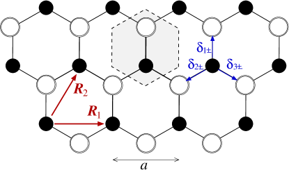
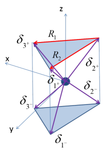
Figure 1: Left panel: Top view of the MoS₂ lattice structure. Dark (light) circles represent Mo (S) atoms. Notice that in this view two S atoms sit on top of each other. The unit cell is shown in the highlighted hexagon. The lattice constant in the Mo plane is $a$. The two Bravais lattice vectors (${\bf R}_{1}$ and ${\bf R}_{2}$) are indicated. Six other auxiliary vectors that connect a Mo atom with its nearest S atoms, ${\bm{\delta}}_{1\pm}$, ${\bm{\delta}}_{2\pm}$, and ${\bm{\delta}}_{3\pm}$, are indicated. Right panel: Tridimensional view of the first neighbors of a Mo atom. The reference trigonal prism coordination unit and other useful quantities are also shown.

For the purpose of building the tight-binding model, we will follow the notation introduced Fig. 1. We denote by “$t$” (or “$+$”) and by “$b$” (or “$-$”) the S atoms at the top and bottom layers, respectively. The distance between the two S layers is $d\cos\theta_{B}=a/\sqrt{3}$. The nearest-neighbour vectors, connecting Mo and S atoms, are given by

$$\bm{\delta}_{1\pm} = d\left(0,\cos\theta_{B},\pm\sin\theta_{B}\right),$$ (3)

$$\bm{\delta}_{2\pm} = d\left(-\frac{\sqrt{3}}{2}\cos\theta_{B},-\frac{1}{2}\cos\theta_{B},\pm\sin\theta_{B}\right),$$ (4)

$$\bm{\delta}_{3\pm} = d\left(+\frac{\sqrt{3}}{2}\cos\theta_{B},-\frac{1}{2}\cos\theta_{B},\pm\sin\theta_{B}\right).$$ (5)

The MoS₂ Brillouin zone is hexagonal. The most important symmetry points and symmetry lines are indicated in Fig. 2, namely, $\Gamma=(0,0)$, $K=\left(\frac{2\pi}{3a},\frac{-2\pi}{\sqrt{3}a}\right)$, and $M=\left(\frac{\pi}{a},\frac{-\pi}{\sqrt{3}a}\right)$. The reciprocal lattice basis vectors are

$${\bf K}_{1}=\frac{4\pi}{\sqrt{3}a}\left(\frac{\sqrt{3}}{2},-\frac{1}{2},0\right)$$ (6)

and

$${\bf K}_{2}=\frac{4\pi}{\sqrt{3}a}\left(0,1,0\right)$$ (7)

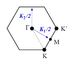
Figure 2: Brillouin zone for the MoS₂ lattice. ${\bf K}_{1}$ and ${\bf K}_{2}$ are the reciprocal lattice basis vectors, and $\Gamma$, $K$, $K^{\prime}$, and $M$ are the high-symmetry points considered in this study.

Table 1: Summary of experimental and theoretical values of the band gap of MoS₂.

Method	Value (eV)	Note
Photoluminescence [8, 29]	1.8-1.9	Optical band gap
Scanning Tunneling Spectrocopy (STS) [31]	2.15
DFT-LDA [36]	1.81
DFT-PBE [37]	1.68
DFT-optB88-vdW [36]	1.67
GW [30]	2.84	G1W0 approximation
DFT-HSE06	2.23	This work

Table 1 summarizes the experimental and theoretical values of the band gap of MoS₂. Early photoluminescence experiments [8, 29] had inferred a direct band gap of about 1.9 eV for MoS₂. More recently, it has been suggested that this value is actually the result of excitonic states and hence corresponds to the optical gap rather than the actual direct gap between the single-particle VB and CB [30]. Scanning Tunneling Spectroscopy (STS) measurements revealed that the band gap of MoS₂ is 2.15 eV [31]. Given the optical gap of about 1.9 eV, the latter value is quite consistent with both theoretical and experimental values of the exciton binding energy, which fall in the range 0.28–0.33 eV according to theory [32, 33] and are either 0.44 eV [34] or 0.22 eV [31] as deduced from experiments. Traditional DFT functionals based on the local density approximation (LDA) and on the generalized gradient approximation (GGA), not surprisingly, underestimate this band gap [35, 36, 37], while the more advanced GW approach tends to overestimate it [30]. The HSE06 functional [20, 21], on the other hand, provides so far the best agreement [38] with the STS result for this gap [31].

In this work, we have therefore chosen the DFT-HSE06 band structure as reference for our fitting procedures. Our DFT-based electronic band structure calculations are carried with the HSE06 functional using the supercell method with a plane-wave basis set (cutoff energy of 500 eV) and the projector-augmented wave (PAW) technique [39, 40], as implemented in the Vienna ab-initio Simulation Package (VASP) [41, 42]. We use a supercell consisting of a MoS₂ layer with an experimental lattice parameter value of 3.16 Å at its center and a vacuum of 15 Å  to minimize the interaction between normal periodical images. The structure is optimized using the GGA approximation with the Perdew-Burke-Ernzerhof (PBE) parameterization [24]. The Brillouin zone is sampled by a $18\times 18\times 1$ mesh. In calculations including spin-orbit-coupling, we sample the Brillouin Zone with a $9\times 9\times 1$ $k$-point mesh to reduce computational cost. The electronic band structure along the $\Gamma$–$K$–$M$–$\Gamma$ directions is calculated with 149 $k$-points and then projected onto every orbital of each atom to resolve the symmetry characters of the corresponding wave-functions. The resulting band structure for a MoS₂ monolayer is shown in Fig. 3.

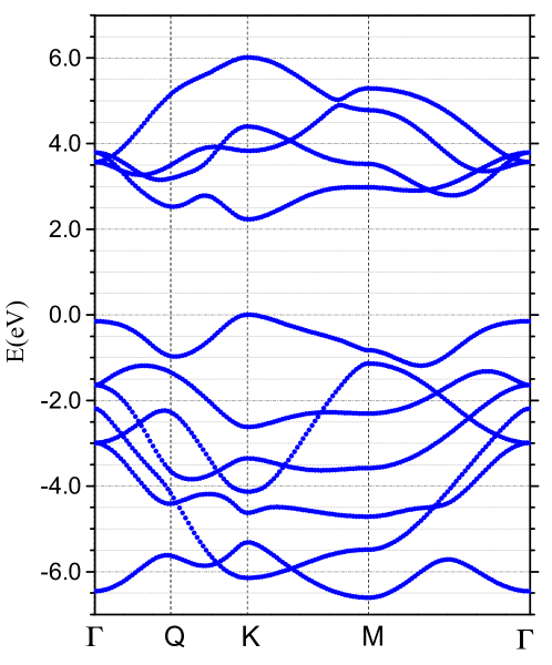
Figure 3: The DFT-HSE06 band structure of MoS₂ near the gap region. See text for details.

Let us summarize the main features near the high-symmetry points of the Brillouin zone [43, 16]:

• $K$ point – The calculated (DFT-HSE06) band gap $E_{G}=2.23$ eV is located at the $K$ point. This result is good agreement with experimental value of 2.15 eV [31]. Electron-hole symmetry is clearly absent: While the effective mass $m_{e}$ in the CB is nearly isotropic, in the VB band it is characterised by a strong trigonal warping. Spin splitting is present in both CB and VB, but the splitting of the VB states is much larger. The VB spin splitting at the $K$ point is experimentally found to be around $145$ meV. Here we only consider spin-orbit coupling up to first order in the coupling and hence disregard the spin splitting in the CB at the $K$ point. Higher order SOC effects have been studied in Refs. [44, 45].

• $Q$ point – This point, signaling a local minimum in the CB band along the straight line connecting $\Gamma$ and $K$ points, has recently received increased attention due to its relevance for transport properties, since the energy minimum $E_{Q}$ is close to the bottom of the CB [15, 43]. From our DFT-HSE06 calculations, before including SOC, we estimate this energy difference to be $\Delta E\approx 0.3$ eV. It is noteworthy that the CB at the $Q$ point moves down in energy in multilayer systems. As discussed in Ref. [26], phonon-limited mobility depends quite sensitively on this energy separation. At the $Q$ point, the CB is characterized by a spin splitting of $91$ meV and the effective mass has an ellipsoidal shape [15]. The $Q$ point is located close to the mid point between $\Gamma$ and $K$ points.

• $\Gamma$ point – This point lies close to the top of the valence band. According to our DFT-HSE06 calculations, before including SOC, its energy difference to the $K$ point is very small, namely, $\Delta E\approx 0.15$ eV. Hence, in hole-doped samples states both the $K$ and $\Gamma$ points will contribute to the electronic transport.

The orbital composition is of fundamental importance for building of any tight-binding model. As already found in literature [25], $d_{xy},d_{x^{2}-y^{2}},d_{z^{2}}$, and $p_{x,y}$ are the most important orbitals to describe the valence and the conduction bands. It is worth to stress that $d_{yz}$ and $d_{xz}$ have a dominant contribution at the $\Gamma$ point, and $p_{z}$ gives an important contribution to both $\Gamma$ and $Q$ points. Thus, for a comprehensive description of the CB and VB along the Brillouin zone, one needs to consider all these orbitals. Tables 2 and 3 show the relative contribution from each orbital at the points $\Gamma$ and $K$, as provided by our DFT-HSE06 calculations. These results serve not only to justify the choice of the relevant orbitals of the atomistic model, but also help in finding the right constraints to optimize the tight-binding parameters.

Table 2: Density functional theory (DFT-HSE06) orbital composition at the $\Gamma$ point for different bands. Absence of an entry indicates zero contribution.

band	band
number	energy (eV)	$p_{y}$	$p_{z}$	$p_{x}$	$d_{xy}$	$d_{yz}$	$d_{z^{2}}$	$d_{xz}$	$d_{x^{2}}$
6	-7.571		0.252				0.199
7	-4.105	0.115		0.127	0.309				0.279
8	-4.105	0.127		0.115	0.279				0.309
9	-3.303		0.558
10	-2.753	0.009		0.313		0.015		0.502
11	-2.753	0.313		0.009		0.502		0.015
12 VB	-1.262		0.141				0.596
13 CB	2.457	0.302		0.045		0.327		0.049
14	2.457	0.045		0.303		0.048		0.327
15	2.678	0.083		0.390	0.249				0.053
16	2.678	0.390		0.083	0.053				0.249

Table 3: Density functional theory (DFT-HSE06) orbital composition at the $K$ point for different bands. Absence of an entry indicates zero contribution.

band	band
number	energy (eV)	$p_{y}$	$p_{z}$	$p_{x}$	$d_{xy}$	$d_{yz}$	$d_{z^{2}}$	$d_{xz}$	$d_{x^{2}}$
6	-7.259	0.155		0.155		0.184		0.184
7	-6.427	0.178		0.178			0.135
8	-5.742	0.231		0.231	0.034				0.034
9	-5.244	0.034	0.359	0.034	0.105				0.105
10	-4.466	0.230	0.129	0.230
11	-3.734	0.416			0.140		0.140
12 VB	-1.111	0.065		0.065	0.345				0.345
13 CB	1.120	0.034		0.034			0.753
14	2.718	0.068		0.068		0.248		0.248
15	3.284	0.016	0.153	0.016	0.327				0.327
16	4.899		0.188			0.303		0.303

3 Model

Let ${\bf r}_{i}$ denote the Mo atom location in the $i$th unit cell. Following Cappelluti and collaborators [25, 26], we consider a tight-binding model with five ${d}$ orbitals in the Mo atom, namely,

$$|{\bf r}_{i};d_{0}\rangle=|d_{3z^{2}-r^{2}}\rangle,\ \ |{\bf r}_{i};d_{1}\rangle=|d_{x^{2}-y^{2}}\rangle,\ \ |{\bf r}_{i};d_{2}\rangle=|d_{xy}\rangle,\ \ |{\bf r}_{i};d_{3}\rangle=|d_{xz}\rangle,\ \ |{\bf r}_{i};d_{4}\rangle=|d_{yz}\rangle,$$

and six $p$ orbitals for the S atoms, three for the top $t$ ($+$) and three for the bottom $b$ ($-$) layers,

$$|{\bf r}_{i}+{\bm{\delta}}_{1\pm};p_{1}\rangle=|p_{x}^{t,b}\rangle,\ \ |{\bf r}_{i}+{\bm{\delta}}_{1\pm};p_{2}\rangle=|p_{y}^{t,b}\rangle,\ \ |{\bf r}_{i}+{\bm{\delta}}_{1\pm};p_{3}\rangle=|p_{z}^{t,b}\rangle.$$

Starting with this basis we can define on-site energies and hopping amplitudes and write down a tight-binding Hamiltonian. Hereafter we assume that this basis is orthogonal.

The tight-binding Hamiltonian $\mathcal{H}$ contains Mo–S and S–S nearest-neighbor hopping terms (in the same unit cell), as well as Mo–Mo and S–S next-to-nearest-neighbor ones (in adjacent cells). Each Mo has six S nearest neighbors. while the next-to-nearest neighbor hoppings connect 6 atoms of the same kind, see Fig. 1. Overall, there is a total of 25 hopping matrix elements inside the unit cell and between the unit cell and the adjacent cells.

The hopping amplitudes are written in terms of Slater-Koster (SK) parameters [19]. We incorporate the $x$ and $z$ reflection symmetries in the construction of the basis, when applicable, to reduce the number of terms. We refer to A for a detailed description of the tight-binding Hamiltonian and the transfer integrals. There, we also provide expressions for the hopping amplitudes in terms of the SK integrals $V_{pd\sigma},V_{pd\pi},V_{dd\sigma},V_{dd\delta},V_{dd\pi},V_{pp\sigma}$, and $V_{pp\pi}$. This allows for a significant reduction in the number of fitting parameters of the model.

To find the energy bands we solve the eigenvector equation that, in the Bloch momentum representation, reads

$$\mathcal{H}|{\bf k}\rangle=E_{\sigma}({\bf k})|{\bf k}\rangle,$$ (8)

where the eigenstates $|{\bf k}\rangle$ are expressed in terms of the three-atom basis, namely,

$$|{\bf k}\rangle=\sum_{{\bf r}_{i}}e^{i{\bf k}\cdot{\bf r}_{i}} \left[\sum_{\mu=0}^{4}\alpha_{{\bf k},\mu}|{\bf r}_{i};d_{\mu}\rangle+\right.$$ (9)

$$\left.\;\;\,\sum_{\mu=1}^{3}\left(\beta_{{\bf k},\mu}|{\bf r}_{i}+{\bm{\delta}}_{1-};p_{\mu},\rangle+\tau_{{\bf k},\mu\sigma}|{\bf r}_{i}+{\bm{\delta}}_{1+};p_{\mu}\rangle\right)\right].$$

For the purpose of implementing the eigenvalue equation we project the vector $\mathcal{H}|{\bf k}\rangle$ onto the three-atom basis and write

$$\left(\begin{array}[]{ccc}h^{\rm{Mo}}+V&T^{t}&T^{b}\\ (T^{t})^{\dagger}&h^{{\rm S}}+U&S\\ (T^{b})^{\dagger}&S&h^{{\rm S}}+U\end{array}\right)\left(\begin{array}[]{c}\alpha\\ \tau\\ \beta\end{array}\right)=E\left(\begin{array}[]{c}\alpha\\ \tau\\ \beta\end{array}\right),$$ (10)

where have omitted, for the moment, the spin indices. Explicit expressions for the block matrices $h^{\rm Mo},h^{\rm S},T^{t},T^{b},S,U,$ and $V$ are given in A. The matrices $S,U$ and $V$ are real and symmetric.

The secular equation (10) is sufficient for a numerical evaluation of the band structure. Nonetheless, it is convenient to use symmetry arguments to reduce the the size of the matrices to be diagonalized, allowing us to express analytically the gap and other features of the band structure at $k$ points of interests.

Let us introduce the symmetric and anti-symmetric components

$$\theta_{\bf{k},\nu}=\frac{1}{\sqrt{2}}(\tau_{\bf{k},\nu}+\beta_{\bf{k},\nu})$$ (11)

and

$$\phi_{\bf{k},\nu}=\frac{1}{\sqrt{2}}(\tau_{\bf{k},\nu}-\beta_{\bf{k},\nu}),$$ (12)

that allow us to write the Hamiltonian in the matrix form

$$\left(\begin{array}[]{ccc}h^{\rm{Mo}}&T^{E}&T^{O}\\ T^{E\dagger}&h^{{Sp}}&0\\ T^{O\dagger}&0&h^{{S}m}\end{array}\right)\left(\begin{array}[]{c}\alpha\\ \theta\\ \phi\end{array}\right)=E\left(\begin{array}[]{c}\alpha\\ \theta\\ \phi\end{array}\right).$$ (13)

The eigenvalue problem can be further simplified by rearranging rows and columns through the transformation $\psi\rightarrow\bar{\psi}$, where

$$\psi^{T}=\left(\alpha_{0},\alpha_{1},\alpha_{2},\alpha_{3},\alpha_{4},\theta_{1},\theta_{2},\theta_{3},\phi_{1},\phi_{2},\phi_{3}\right)$$ (14)

and

$$\bar{\psi}^{T}=\left(\alpha_{0},\alpha_{1},\alpha_{2},\theta_{1},\theta_{2},\phi_{3},\alpha_{3},\alpha_{4},\phi_{1},\phi_{2},\theta_{3}\right).$$ (15)

Notice that the first six orbital basis functions are even ($E$) with respect to a $z$-axis inversion, while the last five are odd ($O$). Then, the problem is reduced to two decoupled eigenvalue/eigenvector problems, namely

$$\left(\begin{array}[]{cc}H^{E}&0\\ 0&H^{O}\end{array}\right)\psi=E\psi.$$ (16)

We refer to B for explicit expressions of the matrix elements of $H^{E}$ and $H^{O}$.

4 Optimization of model parameters

Our tight-binding model Hamiltonian has $N_{p}=12$ fitting parameters, namely, five on-site orbital energies ($D_{0},D_{1},D_{2},D_{p}$, and $D_{z}$) and seven SK parameters related to hopping ($V_{pd\pi},V_{pd\sigma},V_{pp\sigma},V_{pp\pi},V_{dd\sigma},V_{dd\pi},$ and $V_{dd\delta}$). These parameters are optimized to reproduce the main characteristics of the low-energy bands we obtained from DFT-HSE06 calculations.

Our main goal is to reproduce the energies, orbital composition, and effective masses of the conduction and valance bands at the $K,Q,$ and $\Gamma$ points. For that purpose we choose a number of representative $k$-points, shown in Fig. 4, and collect the corresponding band energies $E_{n}({\bf k})$, where $n$ is the band index, to built the data set to be fitted. To better describe the conduction and valence energy bands, we give a larger weight to points $({\bf k},E_{n}({\bf k}))$ near the main band gap. In addition, we take a larger concentration of points around $K,Q,$ and $\Gamma$ to reproduce the electron effective mass around these high symmetry-points.

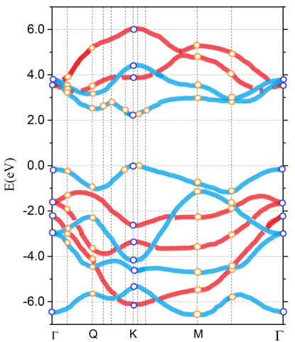
Figure 4: Reference DFT-HSE06 band structure with the constraint points indicated. Blue circles: analytical constraints. Orange circles: numerical constraints. Predominantly even (odd) bands with respect to $z$ inversion are shown in blue (red).

We find the optimal tight-binding parameters using the method of least squares. The data set is built from the band energies $E_{j}^{\rm DFT}$, where $j$ labels both the $k$-point and band index (see Fig. 4), with $j=1,\cdots,N_{f}$. The corresponding $\chi^{2}$-squared function is just a sum of weighted squared residuals, namely,

$$S({\bf P})=\sum_{j=1}^{N_{f}}\frac{\left[E_{j}^{\rm tb}({\bf P})-E_{j}^{\rm DFT}\right]^{2}}{\sigma_{j}^{2}}.$$ (17)

where $\sigma_{j}$ is the weight given to the $j$th data set fitting point, $E_{j}^{\rm tb}({\bf P})$ is the tight-binding energy corresponding to the $j$th data set fitting point. The vector array ${\bf P}$ of dimension $N_{p}$ contains the tight-binding parameters to be minimized. We minimize $S$ with respect to ${\bf P}$ using the Powell method [46], that is an efficient method to find the minimum of a function of several variables without requiring the computation of its derivatives.

Let us briefly describe the route we follow to approximate the low-energy band structure by progressively adding data points.

1. We compare the results obtained at the $K$ and $\Gamma$ points using the analytical expressions derived in C to the DFT-HSE06 energy values and their orbital compositions.

2. We consider $k$ points in the vicinity of $K$ and $\Gamma$. The weights $\sigma$ are adjusted to decrease the importance of these $k$ points as the further away they are from the gap region.

3. We consider additional data points to correctly reproduce other features of the CB and VB. In particular, we add $k$ points at and around the $M$ and $Q$ points, to obtain a correct band energy behavior around the main gap over the entire Brillouin zone.

The tight-binding model Hamiltonian decouples into “even” bands (associated to $H_{E}$) and “odd” bands (associated to $H_{O}$). The identification of the parity of the bands at the $\Gamma$ and $K$ points allows us to follow all the bands over the entire Brillouin zone. Notice that around the main energy gap, bands are mostly even (except for the CB at the $\Gamma$ point). Let us now explain how we match DFT-HSE06 band energies with the tight-binding eigenvalues at the $K$ and $\Gamma$-points.

4.1 $K$ point

At the $K$ point, the matrices $H^{E}$ and $H^{O}$ in Eq. (16) can be written in block diagonal form, namely, we can break $H^{E}$ into three $2\times 2$ diagonal blocks and $H^{O}$ into two $2\times 2$ blocks and one $1\times 1$ block. The explicit expressions are presented in C.

The inspection of the orbital composition given by the DFT-HSE06 calculations (see Table 3) allows us to establish a unique correspondence between pairs of bands and the $2\times 2$ blocks mentioned above. The correspondence is summarized in Table 5.

The identification of the highest $E_{+}$ (lowest $E_{-}$) eigenvalue of a given block with the highest (lowest) energy value of the band with corresponding orbital composition and parity severely constrains our model parameters. By applying this methodology to all diagonal blocks, we find analytical expressions for the band energies at the $K$ point, presented in C.

Table 4: Identification of the tight-binding 2$\times$2 block structures and their orbital contributions at the $K$ point with the band numbers and their corresponding DFT-HSE06 energies, given in Table 3.

block structure orbitals	orbital composition	$(E_{+},E_{-})$ (eV)	band numbers
$H_{E}:\alpha_{0}-\theta_{R}$	$d_{z^{2}},p_{x},p_{y}$	$(1.120,-6.427)$	(13CB, 7)
$H_{E}:\alpha_{L2}-\theta_{L}$	$d_{x^{2}-y^{2}},d_{xy},p_{x},p_{y}$	$(-1.111,-5,742)$	(12VB, 8)
$H_{E}:\alpha_{R2}-\phi_{3}$	$d_{x^{2}-y^{2}}$, $d_{xy}$, $p_{z}$	$(3.284,-5.244)$	(15,9)
$H_{O}:\alpha_{R1}-\phi_{L}$	$d_{yz}$, $d_{xz}$, $p_{x}$,$p_{y}$	$(2.457,-2.753)$	(14,6)
$H_{O}:\alpha_{L1}-\theta_{3}$	$d_{yz}$, $d_{xz}$, $p_{z}$	$(4.899,-3.734)$	(16,11)
$H_{O}:\phi_{R}$	$p_{x},p_{y}$	$-4.466$	10

4.2 $\Gamma$ point

At the $\Gamma$ point we can also express the $H$ matrix of Eq. (16) in block block diagonal form, breaking it into five $2\times 2$ blocks and one $1\times 1$ block.

Here we follow the procedure described in the previous subsection, Sec. 4.1. The differences are due to the distinct point-group symmetries of the $K$ and $\Gamma$ points. As a consequence, the orbital compositions of the tight-binding 2$\times$2 blocks considered in this case are not the same as for the $K$ point. This issue is discussed in C, where we also present the analytical derivation of eigenvalues and eigenstates at the $\Gamma$-point.

Table 5 presents the identification of the tight-binding symmetry split 2$\times$2 blocks with their corresponding DFT-HSE06 bands. It is also noteworthy that, as presented in Table 2, the ad initio calculations show that several band energies coincide at the $\Gamma$ point, namely, 7 and 8, 10 and 11, 13CB and 14, and 15 and 16.

Table 5: Identification of the tight-binding 2$\times$2 block structures and their orbital contributions at the $\Gamma$ point with the band numbers and their corresponding DFT-HSE06 energies, given in Table 2. In the last column, cases where the bands $n_{i},$ and $n_{j}$ have the same energy at the $\Gamma$-point are denoted by $n_{i}$–$n_{j}$.

block structure orbitals	orbital composition	$(E_{+},E_{-})$ (eV)	band numbers
$H_{E}:\alpha_{0}-\phi_{3}$	$d_{z^{2}}$, $p_{z}^{t}$, $p_{z}^{b}$	$(-1.262,-7.571)$	(12VB, 6)
$H_{E}:\alpha_{1}-\theta_{2}$	$d_{x^{2}-y^{2}}$, $p_{x}^{t}$, $p_{x}^{b}$	$(2.678,-4.105)$	(15-16,7-8)
$H_{E}:\alpha_{2}-\theta_{1}$	$p_{y}^{t}$, $p_{y}^{b}$	$(2.678,-4.105)$	(15-16,7-8)
$H_{O}:\alpha_{3}-\phi_{1}$	$d_{xz}$, $p_{x}^{t}$, $p_{x}^{b}$	$(2.457,-2.753)$	(13CB-14,10-11)
$H_{O}:\alpha_{4}-\phi_{2}$	$d_{yz}$, $p_{y}^{t}$, $p_{y}^{b}$	$(2.457,-2.753)$	(13CB-14,10-11)
$H_{O}:\theta_{3}$	$p_{z}^{t}$, $p_{z}^{b}$	$-3.303$	9

5 Eleven-band model: parameters and results

In this Section we present the main results of our study, namely, the tight-binding 11-band parametrization and the corresponding band structure for MoS₂. Table 6 presents the best fitting parameters we obtained using the the optimization procedure described in Sec. 4.

Before discussing the results, it worth mentioning that the even-odd parity symmetry of our tight-binding model prevents a perfect match with ab initio calculations. For instance, DFT-HSE06 calculations indicate that the CB and VB are mainly “even”, but around the $\Gamma$ point they gain a significant odd contribution. Despite this proviso, we show that the tight-binding model reproduces the ab initio band structure close Fermi energy with very good accuracy.

Although our tight-binding model contains many adjustable parameters, the optimization procedure presented in the Sec. 4 imposes several implicit constraints. In practise, we find very difficult to obtain a parameter set that reproduces with high accuracy the position of the energy bands, their orbital compositions, and effective masses at the $K,\Gamma$, and $Q$ points for both CB and VB. For this reason, in Table 6 we present two parameter sets: one that reproduces most features of both VB and CB, but does not yield accurate masses for the VB, and the other that focuses on the VB.

Table 6: Tight-binding model parameters obtained by optimization using $a=3.16\textrm{\AA}$, $\theta_{B}=0.710$, and $d=2.406$ Å. The second column gives the best parameter set we obtain to fit both the valence (VB) and the conduction (CB) bands, while the third column focuses the optimization on the valence band.

parameters	CB-VB optimization (eV)	VB optimization (eV)
$D_{0}$	0.201	0.191
$D_{1}$	-1.563	-1.599
$D_{2}$	-0.352	0.081
$D_{p}$	-54.839	-48.934
$D_{z}$	-39.275	-37.981
$V_{pd\pi}$	4.196	4.115
$V_{pd\sigma}$	-9.880	-8.963
$V_{pp\sigma}$	12.734	10.707
$V_{pp\pi}$	-2.175	-4.084
$V_{dd\sigma}$	-1.153	-1.154
$V_{dd\pi}$	0.612	0.964
$V_{dd\delta}$	0.086	0.117

Figure 5 shows the tight-binding band structure calculated with the VB-CB optimized parameter set given in Table 6 superposed with the DFT-HSE06 result. We find a very good agreement for the conductance and valence bands energies. The accuracy of the tight-binding results becomes increasingly poorer for band energies further away from the gap region, which is expected given that they were attributed a small weight in the fitting procedure.

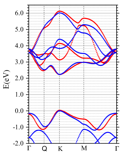
Figure 5: Comparison between the band structures obtained with the DFT-HSE06 (blue) and with the optimized tight-binding model using the parameters from the CB-VB optimization (red) near the gap region.

For completeness, in Table 7 we also include a comparison of the main orbital composition obtained from DFT-HSE06 and the tight-binding result. The orbital compositions at the high symmetry points $\Gamma,K,$ and $Q$ are not equal to those obtained with the DFT-HSE06, but they show the correct leading $d$ and $p$ orbitals for both CB and VB. We point out that this is not the case in the tight-binding parametrization of Ref. [25], where several bands near the main energy gap have incorrect compositions. In particular, at the $K$ point, the correct composition of the VB appears at a high-energy band, far from the gap. In our parametrization, out of the 18 points used in the optimization where analytical expressions where employed, only four yield incorrect compositions and they are located away from the main gap, at low energies.

Table 7: Top: Contribution from each orbital at the $\Gamma$ point using the CB-VB optimization. Bottom: same but at the $K$ point. Omitted orbitals have negligible or null contribution. t-b stands for tight-binding model.

band number
($\Gamma$ point)	$p_{y}$	$p_{z}$	$p_{x}$	$d_{yz}$	$d_{z^{2}}$	$d_{xz}$
DFT-HSE06 12 VB		0.141			0.596
DFT-HSE06 13 CB	0.302		0.045	0.327		0.049
t-b 12 VB		$1.4\cdot 10^{-2}$			0.985
t-b 13 CB	$0.11$		$6.6\cdot 10^{-6}$	0.889		$5.4\cdot 10^{-5}$

band number
($K$ point)	$p_{y}$	$p_{x}$	$d_{xy}$	$d_{z^{2}}$	$d_{x^{2}}$
DFT-HSE06 12 VB	0.065	0.065	0.345		0.345
DFT-HSE06 13 CB	0.034	0.034		0.753
t-b 12 VB	$2.7\cdot 10^{-4}$	$2.7\cdot 10^{-4}$	0.499		0.499
t-b 13 CB	$8.9\cdot 10^{-3}$	$8.9\cdot 10^{-3}$		0.982

Table 8: Effective masses (in units of the free electron mass) at the $\Gamma$ and $K$ points resulting from the CB-VB and the VB optimization.

	HSE06	CB-VB	VB
$\Gamma$ point $m_{e}$	0.76	0.35
$\Gamma$ point $m_{h}$	-2.47	-0.62	-2.47
$K$ point $m_{e}$	0.42	0.58
$K$ point $m_{h}$	-0.47	-0.61	-0.62
$Q$ point $m_{e}$	0.59	0.59

As shown in Table 8, the effective masses are also reasonably well described by the CB-VB parametrization for all three special $k$ points, except for the hole effective mass at the $\Gamma$ point. We try to circumvent this limitation by performing another optimization (named VB) with a heavier weight given to the $k$ values near symmetry points at the VB band. The resulting parametrization describes much more accurately the VB alone, imposing only few distortions on the CB, as Fig. 6 reveals. This procedure yields the VB optimization parameters given in Table 6 and the orbital compositions and effective masses presented in Tables 9 and 8, respectively. Most parameter values are close to those of the global optimization (Table 6), while a few differ by more than 25%. The orbital compositions are nearly identical to those obtained in the global optimization. The most striking change is in the hole band mass the $\Gamma$ point, which become essentically identical to the DFT-HSE06 value.

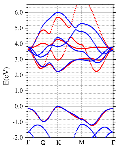
Figure 6: Comparison between the band structures obtained with the DFT-HSE06 (blue) and with the optimized tight-binding model using the parameters from the VB optimization (red) near the gap region. The VB optimization focuses on reproducing accurately the valence band.

Table 9: Top: Contribution from each orbital at the $\Gamma$ point using the parameters from the VB optimization. Bottom: Same but at the $K$ point. Omitted orbitals have negligible or null contribution. t-b stands for tight-binding model.

band number
($\Gamma$ point)	$p_{y}$	$p_{z}$	$p_{x}$	$d_{yz}$	$d_{z^{2}}$	$d_{xz}$
DFT-HSE06 12 VB		0.141			0.596
t-b 12 VB		$1.2\cdot 10^{-2}$			0.988

band number
($K$ point)	$p_{y}$	$p_{x}$	$d_{xy}$	$d_{z^{2}}$	$d_{x^{2}}$
DFT-HSE06 12 VB	0.065	0.065	0.345		0.345
t-b 12 VB	$6.4\cdot 10^{-4}$	$6.4\cdot 10^{-4}$	0.499		0.499

6 Simplified model

The tight-binding model we have developed provides an accurate description of the main features of the CB and VB at the expense of involving a relatively large number of orbitals and fitting parameters. It has already been shown by Liu and coworkers [17] that using just three orbitals for the Mo atom and including only the hopping amplitudes between Mo atoms in plane up to first neighbours is sufficient to open a band gap. With this in mind, we explored whether it is possible to neglect some hopping amplitudes in our tight-binding model and still obtain a reasonable description of the electronic structure near the band gap region. Keeping only the hopping amplitudes between Mo atoms turns out to be insufficient, as it preserves a large amount of degeneracy in the bands. Adding the hopping amplitudes between Mo and neighboring S atoms, without including the hopping amplitudes between S atoms, yields reasonable results. On the other hand, keeping exclusively the Mo–S hoppings does not yield a band gap. In matrix format, this simplified tight-binding model yields the eigenvalue/eigenvector problem

$$\left(\begin{array}[]{ccc}h^{\rm{Mo}}+V&T^{t}&T^{b}\\ (T^{t})^{\dagger}&h^{{S}}&0\\ (T^{b})^{\dagger}&0&h^{{S}}\end{array}\right)\left(\begin{array}[]{c}\alpha\\ \tau\\ \beta\end{array}\right)=E\left(\begin{array}[]{c}\alpha\\ \tau\\ \beta\end{array}\right).$$ (18)

The number of fitting parameters is reduced to from 12 to 10. Symmetries can be fully exploited to break the diagonalization problem into smaller ones, as done previously. After optimization against the DFT-HSE06 band structure, we obtain the values for the fitting parameters listed in Table 10. The resulting band structure is shown in Fig. 7 superposed with the DFT-HSE06 band structure. We note that we were able to reproduce quite well the the entire VB, while the CB is well reproduced just around the $K$ point, missing the correct behaviour aroung the $Q$ and $\Gamma$ points. Therefore, the simplified model is somewhat limited in its applicability. It is suitable for the hole-doped region when the Fermi energy is brought to the top of the VB. It also provides a good description of the system when there is weak electron doping.

Table 10: Parameters for the simplified tight-binding model.

parameter	value (eV)
$D_{0}$	-11.683
$D_{1}$	-208.435
$D_{2}$	-75.942
$D_{p}$	-23.761
$D_{z}$	-35.968
$V_{pdp}$	1.318
$V_{pds}$	-56.738
$V_{dds}$	-2.652
$V_{ddp}$	1.750
$V_{ddd}$	1.482

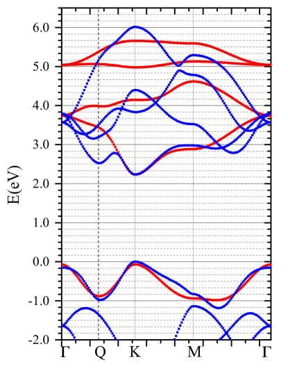
Figure 7: Comparison between the DFT-HSE06 band structure (blue points) and the best fit to the simplified tight-binding model (red points).

7 The effect of spin-orbit interaction

Due to the broken lattice inversion symmetry, strong spin-orbit interactions split the spin-degenerate valence bands in MoS₂ monolayers as well as in other group VI dichalcogenides. The spin-orbit coupling in this case is due to the Dresselhaus mechanism. Interestingly, the spin splitting in inequivalent valleys must be opposite, as imposed by time-reversal symmetry. As mentioned in Sec. 1, these features open interesting possibilities for the control of spins and valleys in these 2D materials [3, 4, 5, 7].

Let us focus on the large spin-splitting at the $K$ point of the VB. Its origin is qualitatively well understood: The valence band states are mostly made of $d_{xy}$ and $d_{x^{2}-y^{2}}$ orbitals with $l=2$ and $m=\pm 2$. Therefore, the $L_{Mo}^{z}S_{Mo}^{z}$ component of the SOC naturally gives a valley-dependent splitting of the bands. In contrast, the dominant contribution of the CB lowest energy state comes from the $d_{z^{2}}$ orbital with $l=2$ and $m=0$, which cancels the spin-orbit splitting. These arguments agree with the quantitative analysis presented in Ref. [44]

A complete tight-binding model that accounts for the effect of SOC over the entire Brillouin zone, including explicitly the $p$-orbitals of the chalcogen atoms, and taking into account the correct orbital composition of the main bands, is lacking.

In this Section, we present an extension of our tight-binding model that includes the effect of an atomic spin-orbit coupling on all the atoms. For that purpose, we follow the formulation presented in Ref. [26]. Our starting point is the 11-band tight-binding spinless model derived earlier, with the Hamiltonian expressed in the appropriate symmetrized form, namely, where the block Hamiltonians $H_{E}$ and $H_{O}$ appear explicitly. The spin-orbit coupling term is inserted in the Hamiltonian by means of a pure intra-atomic spin-orbit interaction acting on all the atoms, explicitly given by

$$H_{\rm SO}=\sum_{a}\frac{\lambda_{a}}{\hbar}\,{\bf L}_{a}\cdot{\bf S}_{a},$$ (19)

where $\lambda_{a}$ is the intrinsic effective SOC constant for an $a$ atom (Mo o S), ${\bf L}_{a}$ is the atomic orbital angular momentum operator, and ${\bf S}_{a}$ is the electronic spin operator. Hence,

$$H=\left(\begin{array}[]{cccc}H_{E}\\ &H_{O}\\ &&H_{E}\\ &&&H_{O}\end{array}\right)+\left(\begin{array}[]{cccc}M_{EE}^{\uparrow\uparrow}&&&M_{EO}^{\uparrow\downarrow}\\ &M_{OO}^{\uparrow\uparrow}&M_{OE}^{\uparrow\downarrow}\\ &M_{EO}^{\downarrow\uparrow}&M_{EE}^{\downarrow\downarrow}\\ M_{OE}^{\downarrow\uparrow}&&&M_{OO}^{\downarrow\downarrow}\end{array}\right)$$ (20)

The matrix elements of $M$ are straightforward to obtain and depend on the SOC parameters $\lambda_{\rm Mo}$ and $\lambda_{\rm S}$. The explicit form of the $M$ matrices can be found in Ref. [26]. We note that in Eq. (20) both diagonal and off-diagonal (spin-flip) terms are taken into account. However, an analysis in Ref. [26] indicates that spin-flip terms have a negligible contribution and could be dropped.

We use DFT-HSE06 to estimate the splittings due to spin-orbit coupling and obtain $\Delta^{K}=202$ meV at the $K$ point of the VB. This value is higher than the experimental one [47], $\Delta_{\rm exp}^{K}=145\pm 4$ meV. This is a known limitation of the HSE06 functional. The strength of this functional relies on its accuracy to predict the band gap of numerous materials, including MoS₂, where traditional DFT calculations (LDA or GGA) give significantly understimated results. Using the SOC values $\lambda_{\rm Mo}=86$ meV and $\lambda_{\rm S}=0.52$ meV, which were obtained from a tight-binding parameter fit to maximally localized Wannier orbitals and to DFT calculations [44], we find $\Delta^{K}=173$ meV. A better result is obtained by adopting the SOC parameters of Cappelluti et al. [26], namely, $\lambda_{\rm Mo}=75$ meV and $\lambda_{\rm S}=0.52$ meV. Inserting these values into our tight-binding formulation results instead in $\Delta^{K}=151$ meV, which is in good agreement with the experimental value. Thus we present in Fig.  8 our results for the spin-resolved band structure based on this choice of SOC parameters.

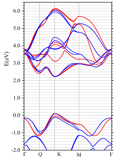
Figure 8: Comparison between the DFT-HSE06 spin-resolved band structure (blue points) and the best-fit tight-binding model (red points). The spin splitting is due to inclusion of spin-orbit coupling.

8 Conclusions

In conclusion, in this paper we provide a suitable and straightforward tight-binding model for a monolayer dichalcogenides, focusing our attention on MoS₂. We show that this model reproduces rather well the structure near the main energy gap provided by an accurate DFT band structure calculation based on the HSE06 functional. It also reproduces the correct orbital composition of the bands. A fundamental ingredient in obtaining this result is the use of an optimization process that makes use of analytical expressions of the energy bands at symmetry points. In the constructing of our model we exploited the decoupling that exists between even and odd bands upon $z$ inversion. Around the main gap, the bands are primarily even. Overall, the model yields 11 bands in the absence of spin-orbit coupling and involves 12 fitting parameters. We provide two parametrizations for this case: one that is suitable for both conduction and valence bands (but less accurate for the valence band), and another that gives a very accurate description of important features of the valence band, such as the effective mass. When spin-orbit coupling is added, the number of fitting parameters jumps to 14. Our choice of parameters in this case yields a spin splitting of the valence band in good agreement with experimental values.

We also investigate the possibility of turning off some hopping amplitudes in our model to reduce the number of parameters to 10 in the absence of spin-orbit coupling. The simplified model is suitable for describing the hole-doped region or when one is only interested in the region around the $K$ point.

The present work provides a sound starting point for any further investigation of electronic transport properties of single-layer semiconductor transition-metal dichalcogenides, or any other investigation that relies heavily on an accurate energy level positioning and wave function composition.

Appendix A Tight-binding model and Slater-Koster parameters

The tight-binding model is defined by the following second-quantized Hamiltonian (spin indices have been omitted):

$$\mathcal{H} = \sum_{{\bf r}_{i}}\sum_{\mu}\varepsilon_{\mu}^{\rm{Mo}}\,d_{i,\mu}^{\dagger}\,d_{i,\mu}$$ (21)

$$+\sum_{{\bf r}_{i}}\sum_{\nu}\varepsilon_{\nu}^{S}\left[\left(p_{i,\nu}^{t}\right)^{\dagger}p_{i,\nu}^{t}+\left(p_{i,\nu,\sigma}^{b}\right)^{\dagger}\,p_{i,\nu}^{b}\right]$$

$$+\sum_{{\bf r}_{i}}\sum_{\mu,\nu}\left[t_{\mu\nu}^{t}\,d_{i,\mu}^{\dagger}\,p_{i,\nu}^{t}+t_{\mu\nu}^{b}\,d_{i,\mu}^{\dagger}\,p_{i,\nu}^{b}+{\rm H.c.}\right]$$

$$+\sum_{{\bf r}_{i}}\sum_{{\bf r}_{j}={\bf r}_{i}+{\bf R}_{1}-{\bf R}_{2}}\sum_{\mu,\nu}\left[t_{\mu\nu}^{r,t}\,d_{i,\mu}^{\dagger}\,p_{j,\nu}^{t}+t_{\mu\nu}^{r,b}\,d_{i,\mu}^{\dagger}\,p_{j,\nu}^{b}+{\rm H.c.}\right]$$

$$+\sum_{{\bf r}_{i}}\sum_{{\bf r}_{j}={\bf r}_{i}-{\bf R}_{2}}\sum_{\mu,\nu}\left[t_{\mu\nu}^{l,t}\,d_{i,\mu}^{\dagger}\,p_{j,\nu}^{t}+t_{\mu\nu}^{l,b}\,d_{i,\mu}^{\dagger}\,p_{j,\nu}^{b}+{\rm H.c.}\right]$$

$$+\sum_{{\bf r}_{i}}\sum_{\nu,\nu^{\prime}}\left[s_{\nu\nu^{\prime}}\left(p_{i,\nu}^{t}\right)^{\dagger}p_{i,\nu^{\prime}}^{b}+{\rm H.c.}\right]$$

$$+\sum_{\langle ij\rangle}\sum_{\mu,\mu^{\prime}}\left[v_{\mu\mu^{\prime}}^{ij}\,d_{i,\mu}^{\dagger}\,d_{j,\mu^{\prime}}+{\rm H.c.}\right]$$

$$+\sum_{\langle ij\rangle}\sum_{\nu,\nu^{\prime}}\left\{u_{\nu\nu^{\prime}}^{ij}\left[\left(p_{i,\nu}^{t}\right)^{\dagger}p_{j,\nu^{\prime}}^{t}+\left(p_{i,\nu}^{b}\right)^{\dagger}p_{j,\nu^{\prime}}^{b}\right]+{\rm H.c.}\right\},$$

where $\langle ij\rangle$ denotes a sum over pairs of nearest-neighbour cells. The operators $d_{i,\mu}$ ($d_{i,\mu}^{\dagger}$) annihilate (create) an electron on the Mo in the unit cell $i$ in the orbital $\mu$. Similarly, the operators $p_{i,\nu}^{b}$ [$(p_{i,\nu}^{b})^{\dagger}$] and $p_{i,\nu}^{t}$ [$(p_{i,\nu}^{t})^{\dagger}$] annihilate (create) electrons at the bottom $b$ and top $t$ S sites of the unit cell $i$, respectively. We assume that the top and bottom S layers are symmetric ($z$ inversion symmetry).

We use the basis set defined in Sec. 3 to express the on-site energies and the hopping integrals. The on-site energies are given by

$$\varepsilon_{\mu}^{\rm{Mo}}=\langle{\bf r}_{i};d_{\mu}|\mathcal{H}|{\bf r}_{i};d_{\mu}\rangle$$ (22)

and

$$\varepsilon_{\nu}^{{S}}=\langle{\bf r}_{i}+{\bm{\delta}}_{1\pm};p_{\nu}|\mathcal{H}|{\bf r}_{i}+{\bm{\delta}}_{1\pm};p_{\nu}\rangle.$$ (23)

The hopping matrix elements between Mo and S orbitals are

$$t_{\mu\nu}^{t} = \langle{\bf r}_{i};d_{\mu}|\mathcal{H}|{\bf r}_{i}+{\bm{\delta}}_{1+};p_{\nu}\rangle,$$ (24)

$$t_{\mu\nu}^{b} = \langle{\bf r}_{i};d_{\mu}|\mathcal{H}|{\bf r}_{i}+{\bm{\delta}}_{1-};p_{\nu}\rangle,$$ (25)

$$t_{\mu\nu}^{r,t} = \langle{\bf r}_{i};d_{\mu}|\mathcal{H}|{\bf r}_{i}+{\bf R}_{1}-{\bf R}_{2}+{\bm{\delta}}_{1+};p_{\nu}\rangle,$$ (26)

$$t_{\mu\nu}^{r,b} = \langle{\bf r}_{i};d_{\mu}|\mathcal{H}|{\bf r}_{i}+{\bf R}_{1}-{\bf R}_{2}+{\bm{\delta}}_{1-};p_{\nu}\rangle,$$ (27)

$$t_{\mu\nu}^{l,t} = \langle{\bf r}_{i};d_{\mu}|\mathcal{H}|{\bf r}_{i}-{\bf R}_{2}+{\bm{\delta}}_{1+};p_{\nu}\rangle,$$ (28)

$$t_{\mu\nu}^{l,b} = \langle{\bf r}_{i};d_{\mu}|\mathcal{H}|{\bf r}_{i}-{\bf R}_{2}+{\bm{\delta}}_{1-};p_{\nu}\rangle.$$ (29)

The hopping matrix elements between top and bottom S orbitals read

$$s_{\nu\nu^{\prime}} = \langle{\bf r}_{i}+{\bm{\delta}}_{1+};p_{\mu}|\mathcal{H}|{\bf r}_{i}+{\bm{\delta}}_{1-};p_{\nu^{\prime}}\rangle,$$ (30)

while the nearest-neighbor Mo-Mo hopping integrals are

$$v_{\mu\mu^{\prime}}^{{E}} = \langle{\bf r}_{i};d_{\mu}|\mathcal{H}|{\bf r}_{i}+{\bf R}_{1};d_{\mu^{\prime}}\rangle,$$ (31)

$$v_{\mu\mu^{\prime}}^{\rm{NE}} = \langle{\bf r}_{i};d_{\mu}|\mathcal{H}|{\bf r}_{i}+{\bf R}_{2};d_{\mu^{\prime}}\rangle,$$ (32)

$$v_{\mu\mu^{\prime}}^{\rm{NW}} = \langle{\bf r}_{i};d_{\mu}|\mathcal{H}|{\bf r}_{i}+{\bf R}_{2}-{\bf R}_{1};d_{\mu^{\prime}}\rangle,$$ (33)

$$v_{\mu\mu^{\prime}}^{{W}} = \langle{\bf r}_{i};d_{\mu}|\mathcal{H}|{\bf r}_{i}-{\bf R}_{1};d_{\mu^{\prime}}\rangle,$$ (34)

$$v_{\mu\mu^{\prime}}^{\rm{SW}} = \langle{\bf r}_{i};d_{\mu}|\mathcal{H}|{\bf r}_{i}-{\bf R}_{2};d_{\mu^{\prime}}\rangle,$$ (35)

$$v_{\mu\mu^{\prime}}^{\rm{SE}} = \langle{\bf r}_{i};d_{\mu}|\mathcal{H}|{\bf r}_{i}-{\bf R}_{2}+{\bf R}_{1};d_{\mu^{\prime}}\rangle,$$ (36)

and the S–S next-nearest-neighbor hopping matrix elements read

$$u_{\nu\nu^{\prime}}^{\rm{E}} = \langle{\bf r}_{i}+{\bm{\delta}}_{1\pm};p_{\nu}|\mathcal{H}|{\bf r}_{i}+{\bf R}_{1}+{\bm{\delta}}_{1\pm};p_{\nu^{\prime}}\rangle,$$ (38)

$$u_{\nu\nu^{\prime}}^{\rm{NE}} = \langle{\bf r}_{i}+{\bm{\delta}}_{1\pm};p_{\nu}|\mathcal{H}|{\bf r}_{i}+{\bf R}_{2}+{\bm{\delta}}_{1\pm};p_{\nu^{\prime}}\rangle,$$ (39)

$$u_{\nu\nu^{\prime}}^{\rm{NW}} = \langle{\bf r}_{i}+{\bm{\delta}}_{1\pm};p_{\nu}|\mathcal{H}|{\bf r}_{i}+{\bf R}_{2}-{\bf R}_{1}+{\bm{\delta}}_{1\pm};p_{\nu^{\prime}}\rangle,$$ (40)

$$u_{\nu\nu^{\prime}}^{{W}} = \langle{\bf r}_{i}+{\bm{\delta}}_{1\pm};p_{\nu}|\mathcal{H}|{\bf r}_{i}-{\bf R}_{1}+{\bm{\delta}}_{1\pm};p_{\nu^{\prime}}\rangle,$$ (41)

$$u_{\nu\nu^{\prime}}^{\rm{SW}} = \langle{\bf r}_{i}+{\bm{\delta}}_{1\pm};p_{\nu}|\mathcal{H}|{\bf r}_{i}-{\bf R}_{2}+{\bm{\delta}}_{1\pm};p_{\nu^{\prime}}\rangle,$$ (42)

$$u_{\nu\nu^{\prime}}^{\rm{SE}} = \langle{\bf r}_{i}+{\bm{\delta}}_{1\pm};p_{\nu}|\mathcal{H}|{\bf r}_{i}-{\bf R}_{2}+{\bf R}_{1}+{\bm{\delta}}_{1\pm};p_{\nu^{\prime}}\rangle.$$ (43)

Notice that $\mathcal{H}$ contains Mo–S and S–S nearest-neighbour (same unit cell) hopping amplitudes and Mo–Mo and S–S next-to-nearest-neighbour hopping amplitudes (adjacent cells). For the latter, each Mo and each S has six next-to-nearest neighbours. For the former, each Mo has six S nearest neighbours. Overall, there is a total of 25 hopping amplitudes within the unit cell and between the unit cell and the adjacent cells. The hopping amplitudes are indicated in Fig. 9.

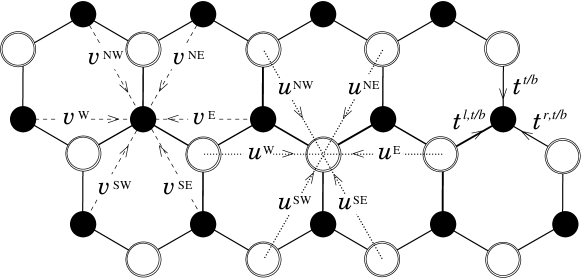
Figure 9: Scheme of the hopping amplitudes. Solid black circles represent Mo atoms, while empty circles represent the S atoms at the top and bottom layers.

The following associations are made for the on-site energies of Mo atoms: $\varepsilon_{0}^{\rm{Mo}}\equiv\Delta_{0}$, $\varepsilon_{1}^{\rm{Mo}}=\varepsilon_{2}^{\rm{Mo}}\equiv\Delta_{2}$, $\varepsilon_{3}^{\rm{Mo}}=\varepsilon_{4}^{\rm{Mo}}\equiv\Delta_{1}$. For on-site energies of the S atoms we define $\varepsilon_{1}^{{S}}=\varepsilon_{2}^{{S}}\equiv\Delta_{p}$ and $\varepsilon_{3}^{{S}}\equiv\Delta_{z}$.

The hopping amplitudes can be written in terms of SK integrals. We can also incorporate the $x$ and $z$ reflection symmetries, when applicable, to reduce the number of terms. Here we provide expressions for the more relevant hopping amplitudes in terms of seven SK integrals. This allows us to substantially reduce the number of fitting parameters of the model. Below we list amplitudes that are not identically zero.

• Mo–S (Here we present the expressions for the $t^{t}$ hopping matrix elements. The $t^{b}$ ones follow similar expressions, with $\theta_{b}\leftrightarrow-\theta_{b}$.)

  $$\hskip-99.58464ptt_{02}^{t}=\cos\theta_{b}\left(\sin^{2}\theta_{b}-\frac{1}{2}\cos^{2}\theta_{b}\right)V_{pd\sigma}-\sqrt{3}\cos\theta_{b}\sin^{2}\theta_{b}V_{pd\pi},$$ (44)

  $$\hskip-99.58464ptt_{03}^{t}=\sin\theta_{b}\left(\sin^{2}\theta_{b}-\frac{1}{2}\cos^{2}\theta_{b}\right)V_{pd\sigma}+\sqrt{3}\sin\theta_{b}\cos^{2}\theta_{b}V_{pd\pi},$$ (45)

  $$\hskip-99.58464ptt_{12}^{t}=-\frac{\sqrt{3}}{2}\cos^{3}\theta_{b}V_{pd\sigma}-\cos\theta_{b}\sin^{2}\theta_{b}V_{pd\pi},$$ (46)

  $$\hskip-99.58464ptt_{13}^{t}=-\sin\theta_{b}\cos^{2}\theta_{b}\left(\frac{\sqrt{3}}{2}V_{pd\sigma}-V_{pd\pi}\right),$$ (47)

  $$\hskip-99.58464ptt_{21}^{t}=\cos\theta_{b}V_{pd\pi},$$ (48)

  $$\hskip-99.58464ptt_{31}^{t}=\sin\theta_{b}V_{pd\pi},$$ (49)

  $$\hskip-99.58464ptt_{42}^{t}=\sqrt{3}\cos^{2}\theta_{b}\sin\theta_{b}V_{pd\sigma}+\sin\theta_{b}(1-2\cos^{2}\theta_{b})V_{pd\pi},$$ (50)

  $$\hskip-99.58464ptt_{43}^{t}=\sqrt{3}\sin^{2}\theta_{b}\cos\theta_{b}V_{pd\sigma}+\cos\theta_{b}(1-2\sin^{2}\theta_{b})V_{pd\pi},$$ (51)

  $$\hskip-99.58464ptt_{01}^{l,t}=-\frac{\sqrt{3}}{2}\cos\theta_{b}\left(\sin^{2}\theta_{b}-\frac{1}{2}\cos^{2}\theta_{b}\right)V_{pd\sigma}+\frac{3}{2}\cos\theta_{b}\sin^{2}\theta_{b}V_{pd\pi},$$ (52)

  $$\hskip-99.58464ptt_{02}^{l,t}=-\frac{1}{2}\cos\theta_{b}\left(\sin^{2}\theta_{b}-\frac{1}{2}\cos^{2}\theta_{b}\right)V_{pd\sigma}+\frac{\sqrt{3}}{2}\cos\theta_{b}\sin^{2}\theta_{b}V_{pd\pi},$$ (53)

  $$\hskip-99.58464ptt_{03}^{l,t}=\sin\theta_{b}\left(\sin^{2}\theta_{b}-\frac{1}{2}\cos^{2}\theta_{b}\right)V_{pd\sigma}+\sqrt{3}\sin\theta_{b}\cos^{2}\theta_{b}V_{pd\pi},$$ (54)

  $$\hskip-99.58464ptt_{11}^{l,t}=-\frac{3}{8}\cos^{3}\theta_{b}V_{pd\sigma}-\frac{\sqrt{3}}{2}\cos\theta_{b}\left(1-\frac{1}{2}\cos^{2}\theta_{b}\right)V_{pd\pi},$$ (55)

  $$\hskip-99.58464ptt_{12}^{l,t}=-\frac{\sqrt{3}}{8}\cos^{3}\theta_{b}V_{pd\sigma}+\frac{1}{2}\cos\theta_{b}\left(1+\frac{1}{2}\cos^{2}\theta_{b}\right)V_{pd\pi},$$ (56)

  $$\hskip-99.58464ptt_{13}^{l,t}=\frac{1}{2}\sin\theta_{b}\cos^{2}\theta_{b}\left(\frac{\sqrt{3}}{2}V_{pd\sigma}-V_{pd\pi},\right)$$ (57)

  $$\hskip-99.58464ptt_{21}^{l,t}=-\frac{3\sqrt{3}}{8}\cos^{3}\theta_{b}V_{pd\sigma}-\frac{1}{2}\cos\theta_{b}\left(1-\frac{3}{2}\cos^{2}\theta_{b}\right)V_{pd\pi},$$ (58)

  $$\hskip-99.58464ptt_{22}^{l,t}=-\frac{3}{8}\cos^{3}\theta_{b}V_{pd\sigma}-\frac{\sqrt{3}}{2}\cos\theta_{b}\left(1-\frac{1}{2}\cos^{2}\theta_{b}\right)V_{pd\pi},$$ (59)

  $$\hskip-99.58464ptt_{23}^{l,t}=\frac{\sqrt{3}}{4}\sin\theta_{b}\cos^{2}\theta_{b}\left(\sqrt{3}V_{pd\sigma}-2V_{pd\pi}\right),$$ (60)

  $$\hskip-99.58464ptt_{31}^{l,t}=\frac{3\sqrt{3}}{4}\cos^{2}\theta_{b}\sin\theta_{b}V_{pd\sigma}+\sin\theta_{b}\left(1-\frac{3}{2}\cos^{2}\theta_{b}\right)V_{pd\pi},$$ (61)

  $$\hskip-99.58464ptt_{32}^{l,t}=\frac{\sqrt{3}}{4}\sin\theta_{b}\cos^{2}\theta_{b}\left(\sqrt{3}V_{pd\sigma}-2V_{pd\pi}\right),$$ (62)

  $$\hskip-99.58464ptt_{33}^{l,t}=-\frac{3}{2}\sin^{2}\theta_{b}\cos\theta_{b}V_{pd\sigma}-\frac{\sqrt{3}}{2}\cos\theta_{b}\left(1-2\sin^{2}\theta_{b}\right)V_{pd\pi},$$ (63)

  $$\hskip-99.58464ptt_{41}^{l,t}=\frac{\sqrt{3}}{4}\sin\theta_{b}\cos^{2}\theta_{b}\left(\sqrt{3}V_{pd\sigma}-2V_{pd\pi}\right),$$ (64)

  $$\hskip-99.58464ptt_{42}^{l,t}=\frac{\sqrt{3}}{4}\cos^{2}\theta_{b}\sin\theta_{b}V_{pd\sigma}+\sin\theta_{b}\left(1-\frac{1}{2}\cos^{2}\theta_{b}\right)V_{pd\pi},$$ (65)

  $$\hskip-99.58464ptt_{43}^{l,t}=-\frac{\sqrt{3}}{2}\sin^{2}\theta_{b}\cos\theta_{b}V_{pd\sigma}-\frac{1}{2}\cos\theta_{b}\left(1-2\sin^{2}\theta_{b}\right)V_{pd\pi}.$$ (66)

• Mo–Mo ($v^{W}$, $v^{NW}$, $v^{SW}$ and $s^{SE}$ can be obtained from $v^{E}$ and $v^{NE}$ by symmetry.)

  $$\hskip-99.58464ptv_{00}^{{E}}=\frac{1}{4}V_{dd\sigma}+\frac{3}{4}V_{dd\delta},$$ (67)

  $$\hskip-99.58464ptv_{01}^{{E}}=-\frac{\sqrt{3}}{4}V_{dd\sigma}+\frac{\sqrt{3}}{4}V_{dd\delta},$$ (68)

  $$\hskip-99.58464ptv_{11}^{{E}}=\frac{3}{4}V_{dd\sigma}+\frac{1}{4}V_{dd\delta}$$ (69)

  $$\hskip-99.58464ptv_{22}^{{E}}=V_{dd\pi},$$ (70)

  $$\hskip-99.58464ptv_{33}^{{E}}=V_{dd\pi},$$ (71)

  $$\hskip-99.58464ptv_{44}^{{E}}=V_{dd\delta},$$ (72)

  $$\hskip-99.58464ptv_{02}^{\rm{NE}}=-\frac{3}{8}V_{dd\sigma}+\frac{3}{8}V_{dd\delta},$$ (73)

  $$\hskip-99.58464ptv_{12}^{\rm{NE}}=-\frac{3\sqrt{3}}{16}V_{dd\sigma}+\frac{\sqrt{3}}{4}V_{dd\pi}-\frac{\sqrt{3}}{16}V_{dd\delta},$$ (74)

  $$\hskip-99.58464ptv_{34}^{\rm{NE}}=\frac{\sqrt{3}}{4}V_{dd\pi}-\frac{\sqrt{3}}{4}V_{dd\delta}.$$ (75)

• S–S ($u^{W}$, $u^{NW}$, $u^{SW}$, and $u^{SE}$ can be obtained from $u^{E}$ and $u^{NE}$ by symmetry.)

  $$\hskip-99.58464ptu_{11}^{{E}}=V_{pp\sigma},$$ (76)

  $$\hskip-99.58464ptu_{22}^{{E}}=V_{pp\pi},$$ (77)

  $$\hskip-99.58464ptu_{33}^{{E}}=V_{pp\pi},$$ (78)

  $$\hskip-99.58464ptu_{12}^{\rm{NE}}=\frac{\sqrt{3}}{4}(V_{pp\sigma}-V_{pp\pi}).$$ (79)

  $$\hskip-99.58464pts_{11}=V_{pp\pi},$$ (80)

  $$\hskip-99.58464pts_{22}=V_{pp\pi},$$ (81)

  $$\hskip-99.58464pts_{33}=V_{pp\sigma}.$$ (82)

A general yet compact expression for all amplitudes is given by the matrices

$$\hskip-99.58464ptt^{t}=\left(\begin{array}[]{ccc}0&t^{t}_{02}&t^{t}_{03}\\ 0&t^{t}_{12}&t^{t}_{13}\\ t^{t}_{21}&0&0\\ t^{t}_{31}&0&0\\ 0&t^{t}_{42}&t^{t}_{43}\end{array}\right),$$ (83)

$$\hskip-99.58464ptt^{b}=\left(\begin{array}[]{ccc}0&t^{t}_{02}&-t_{03}^{t}\\ 0&t_{12}^{t}&-t_{13}^{t}\\ t_{21}^{t}&0&0\\ -t_{31}^{t}&0&0\\ 0&-t_{42}^{t}&t_{43}^{t}\end{array}\right),$$ (84)

$$\hskip-99.58464ptt^{l,t}=\left(\begin{array}[]{ccc}t_{01}^{l,t}&t^{l,t}_{02}&t^{l,t}_{03}\\ t_{11}^{l,t}&t^{l,t}_{12}&t^{l,t}_{13}\\ t^{l,t}_{21}&t_{22}^{l,t}&t_{23}^{l,t}\\ t^{l,t}_{31}&t_{32}^{l,t}&t_{33}^{l,t}\\ t_{41}^{l,t}&t^{l,t}_{42}&t^{l,t}_{43}\end{array}\right),$$ (85)

$$\hskip-99.58464ptt^{l,b}=\left(\begin{array}[]{ccc}t_{01}^{l,t}&t^{l,t}_{02}&-t^{l,t}_{03}\\ t_{11}^{l,t}&t^{l,t}_{12}&-t^{l,t}_{13}\\ t^{l,t}_{21}&t_{22}^{l,t}&-t_{23}^{l,t}\\ -t^{l,t}_{31}&-t_{32}^{l,t}&t_{33}^{l,t}\\ -t_{41}^{l,t}&-t^{l,t}_{42}&t^{l,t}_{43}\end{array}\right),$$ (86)

$$\hskip-99.58464ptt^{r,t}=\left(\begin{array}[]{ccc}-t_{01}^{l,t}&t^{l,t}_{02}&t^{l,t}_{03}\\ -t_{11}^{l,t}&t^{l,t}_{12}&t^{l,t}_{13}\\ t^{l,t}_{21}&-t_{22}^{l,t}&-t_{23}^{t{L}}\\ t^{l,t}_{31}&-t_{32}^{l,t}&-t_{33}^{l,t}\\ -t_{41}^{l,t}&t^{l,t}_{42}&t^{l,t}_{43}\end{array}\right),$$ (87)

$$\hskip-99.58464ptt^{r,b}=\left(\begin{array}[]{ccc}-t_{01}^{l,t}&t^{l,t}_{02}&-t^{l,t}_{03}\\ -t_{11}^{l,t}&t^{l,t}_{12}&-t^{l,t}_{13}\\ t^{l,t}_{21}&-t_{22}^{l,t}&t_{23}^{l,t}\\ -t^{l,t}_{31}&t_{32}^{l,t}&-t_{33}^{l,t}\\ t_{41}^{l,t}&-t^{l,t}_{42}&t^{l,t}_{43}\end{array}\right),$$ (88)

$$\hskip-99.58464ptv^{{E}}=\left(\begin{array}[]{ccccc}v^{{E}}_{00}&v^{{E}}_{01}&0&0&0\\ v^{{E}}_{01}&v^{E}_{11}&0&0&0\\ 0&0&v^{{E}}_{22}&0&0\\ 0&0&0&v^{{E}}_{33}&0\\ 0&0&0&0&v^{{E}}_{44}\end{array}\right),$$ (89)

$$\hskip-99.58464ptv^{{W}}=\left(\begin{array}[]{ccccc}v^{{E}}_{00}&v^{{E}}_{01}&0&0&0\\ v^{{E}}_{01}&v^{E}_{11}&0&0&0\\ 0&0&v^{{E}}_{22}&0&0\\ 0&0&0&v^{{E}}_{33}&0\\ 0&0&0&0&v^{{E}}_{44}\end{array}\right),$$ (90)

$$\hskip-99.58464ptv^{{NE}}=\left(\begin{array}[]{ccccc}v_{00}^{E}&-\frac{1}{2}v_{01}^{E}&v_{02}^{{NE}}&0&0\\ -\frac{1}{2}v_{01}^{E}&\frac{1}{4}v_{11}^{{E}}+\frac{3}{4}v_{22}^{{E}}&v_{12}^{{NE}}&0&0\\ v_{02}^{{NE}}&v_{12}^{{NE}}&\frac{1}{4}v_{22}^{{E}}+\frac{3}{4}v_{11}^{{E}}&0&0\\ 0&0&0&\frac{1}{4}v_{33}^{{E}}+\frac{3}{4}v_{44}^{{E}}&v_{34}^{{NE}}\\ 0&0&0&v_{34}^{{NE}}&\frac{1}{4}v_{44}^{{E}}+\frac{3}{4}v_{33}^{{E}}\end{array}\right),$$ (91)

$$\hskip-99.58464ptv^{{NW}}=\left(\begin{array}[]{ccccc}v_{00}^{E}&-\frac{1}{2}v_{01}^{E}&-v_{02}^{{NE}}&0&0\\ -\frac{1}{2}v_{01}^{E}&\frac{1}{4}v_{11}^{{E}}+\frac{3}{4}v_{22}^{{E}}&-v_{12}^{{NE}}&0&0\\ -v_{02}^{{NE}}&-v_{12}^{{NE}}&\frac{1}{4}v_{22}^{{E}}+\frac{3}{4}v_{11}^{{E}}&0&0\\ 0&0&0&\frac{1}{4}v_{33}^{{E}}+\frac{3}{4}v_{44}^{{E}}&-v_{34}^{{NE}}\\ 0&0&0&-v_{34}^{{NE}}&\frac{1}{4}v_{44}^{{E}}+\frac{3}{4}v_{33}^{{E}}\end{array}\right),$$ (92)

$$\hskip-99.58464ptu^{{E}}=\left(\begin{array}[]{ccc}u^{{E}}_{11}&0&0\\ 0&u^{{E}}_{22}&0\\ 0&0&u^{{E}}_{33}\end{array}\right),$$ (93)

$$\hskip-99.58464ptu^{{NE}}=\left(\begin{array}[]{ccc}\frac{1}{4}u_{11}^{{E}}+\frac{3}{4}u_{22}^{{E}}&u_{12}^{{NE}}&0\\ u_{12}^{{NE}}&\frac{1}{4}u_{22}^{{E}}+\frac{3}{4}u_{11}^{{E}}&0\\ 0&0&u_{33}^{{E}}\end{array}\right),$$ (94)

and

$$\hskip-99.58464ptu^{{NW}}=\left(\begin{array}[]{ccc}\frac{1}{4}u_{11}^{{E}}+\frac{3}{4}u_{22}^{{E}}&-u_{12}^{{NE}}&0\\ -u_{12}^{{NE}}&\frac{1}{4}u_{22}^{{E}}+\frac{3}{4}u_{11}^{{E}}&0\\ 0&0&u_{33}^{{E}}\end{array}\right).$$ (95)

Appendix B Tight-binding energy bands

To find the energy bands we need to solve the the eigenvalue/eigenvector problem in the Bloch momentum representation,

$$\mathcal{H}|{\bf k}\rangle=E({\bf k})|{\bf k}\rangle,$$ (96)

where the Bloch vector is given by

$$\hskip-51.21504pt|{\bf k}\rangle = \sum_{{\bf r}_{i}}e^{i{\bf k}\cdot{\bf r}_{i}}\left[\sum_{\mu=0}^{4}\alpha_{{\bf k},\mu}|{\bf r}_{i};d_{\mu}\rangle+\sum_{\mu=1}^{3}\left(\beta_{{\bf k},\mu}|{\bf r}_{i}+{\bm{\delta}}_{1-};p_{\mu}\rangle+\tau_{{\bf k},\mu}|{\bf r}_{i}+{\bm{\delta}}_{1+};p_{\mu}\rangle\right)\right].$$ (97)

Resorting to the orthogonal bais, we can rewrite the eigenvalue/eigenvector problem as a system of linear coupled equations,

$$\hskip-51.21504pt\left[E(\bf{k})-\varepsilon_{{\mu}}^{\rm{Mo}}\right]\alpha_{\bf{k},{\mu}} = \sum_{\nu}\left[\left(t_{{\mu}\nu}^{t}+z_{2}^{\ast}\,t_{{\mu}\nu}^{t{L}}+z_{2}^{\ast}\,z_{1}t_{{\mu}\nu}^{r,t}\right)\tau_{\bf{k},\nu}+\left(t_{{\mu}\nu}^{b}+z_{2}^{\ast}\,t_{{\mu}\nu}^{l,b}+z_{2}^{\ast}\,z_{1}\,t_{{\mu}\nu}^{r,b}\right)\beta_{\bf{k},\nu}\right]$$ (98)

$$+2\sum_{{\mu}^{\prime}}\left(c_{1}\,v_{{\mu}{\mu}^{\prime}}^{{E}}+c_{2}\,v_{{\mu}{\mu}^{\prime}}^{\rm{NE}}+c_{12}\,v_{{\mu}{\mu}^{\prime}}^{\rm{NW}}\right)\alpha_{\bf{k},{\mu}^{\prime}},$$

$$\hskip-51.21504pt\left[E({\bf k})-\varepsilon_{\nu}^{{\rm S}}\right]\beta_{\bf{k},\nu} = \sum_{{\mu}}\left(t_{{\mu}\nu}^{b}+z_{2}t_{{\mu}\nu}^{l,b}+z_{2}\,z_{1}^{\ast}t_{{\mu}\nu}^{r,b}\right)\alpha_{\bf{k},{\mu}}$$ (99)

$$+\sum_{\nu^{\prime}}\left[\left(c_{1}\,u_{\nu\nu^{\prime}}^{{E}}+c_{2}\,u_{\nu\nu^{\prime}}^{\rm{NE}}+c_{12}\,u_{\nu\nu^{\prime}}^{\rm{NW}}\right)\beta_{\bf{k},\nu^{\prime}}+s_{\nu\nu^{\prime}}\,\tau_{\bf{k},\nu^{\prime}}\right],$$

and

$$\hskip-51.21504pt\left[E({\bf k})-\varepsilon_{\nu}^{{\rm S}}\right]\tau_{\bf{k},\nu} = \sum_{{\mu}}\left(t_{{\mu}\nu}^{t}+z_{2}t_{{\mu}\nu}^{t{L}}+z_{2}\,z_{1}^{\ast}t_{{\mu}\nu}^{t{R}}\right)\alpha_{\bf{k},{\mu}}$$ (100)

$$+\sum_{\nu^{\prime}}\left[\left(c_{1}\,u_{\nu\nu^{\prime}}^{{E}}+c_{2}\,u_{\nu\nu^{\prime}}^{\rm{NE}}+c_{12}\,u_{\nu\nu^{\prime}}^{\rm{NW}}\right)\tau_{\bf{k},\nu^{\prime}}+s_{\nu\nu^{\prime}}\beta_{\bf{k},\nu^{\prime}}\right],$$

where $z_{1}=e^{i{\bf k}\cdot{\bf R}_{1}}=e^{iak_{x}}$, $z_{2}=e^{i{\bf k}\cdot{\bf R}_{2}}=e^{iak_{x}/2}e^{i\sqrt{3}ak_{y}/2}$,

$$c_{1}\equiv\frac{z_{1}+z_{1}^{\ast}}{2}=\cos({\bf k}\cdot{\bf R}_{1})=\cos(k_{x}a),$$ (101)

$$c_{2}\equiv\frac{z_{2}+z_{2}^{\ast}}{2}=\cos({\bf k}\cdot{\bf R}_{2})=\cos\left(k_{x}a/2+k_{y}\sqrt{3}a/2\right),$$ (102)

and

$$c_{12}\equiv\frac{z_{1}\,z_{2}^{\ast}+z_{1}^{\ast}\,z_{2}}{2}=\cos({\bf k}\cdot{\bf R}_{1}-{\bf k}\cdot{\bf R}_{2})=\cos\left(k_{x}a/2-k_{y}\sqrt{3}a/2\right).$$ (103)

In matrix form, we have

$$\left(\begin{array}[]{ccc}h^{\rm{Mo}}+V&T^{t}&T^{b}\\ \left(T^{t}\right)^{T}&h^{{S}}+U&s\\ \left(T^{b}\right)^{T}&s&h^{{S}}+U\end{array}\right)\left(\begin{array}[]{c}\alpha\\ \tau\\ \beta\end{array}\right)=E\left(\begin{array}[]{c}\alpha\\ \tau\\ \beta\end{array}\right),$$ (113)

where

$$\hskip-56.9055pth^{\rm{Mo}}=\left(\begin{array}[]{ccccc}\Delta_{0}&0&0&0&0\\ 0&\Delta_{2}&0&0&0\\ 0&0&\Delta_{2}&0&0\\ 0&0&0&\Delta_{1}&0\\ 0&0&0&0&\Delta_{1}\end{array}\right),$$ (114)

$$\hskip-56.9055pth^{{S}}=\left(\begin{array}[]{ccc}\Delta_{p}&0&0\\ 0&\Delta_{p}&0\\ 0&0&\Delta_{z}\end{array}\right),$$ (115)

$$\hskip-56.9055ptT^{t}=t^{t}+z_{2}^{\ast}\left(t^{l,t}+z_{1}\,t^{r,t}\right),$$ (116)

$$\hskip-56.9055ptT^{b}=t^{b}+z_{2}^{\ast}\left(t^{l,b}+z_{1}\,t^{r,b}\right),$$ (117)

$$\hskip-56.9055ptV=2\left(c_{1}\,v^{{E}}+c_{2}\,v^{\rm{NE}}+c_{12}\,v^{\rm{NW}}\right),$$ (118)

and

$$\hskip-56.9055ptU=2\left(c_{1}\,u^{{E}}+c_{2}\,u^{\rm{NE}}+c_{12}\,u^{\rm{NW}}\right).$$ (119)

This formulation suffices for a numerical evaluation of the bands. However, in order to obtain analytical expression for the gap and other features of the band structure at the symmetry points, it is necessary to reduce the size of the matrices to be diagonalized. This can be done by exploring underlying symmetries in the equations.

Let us define the symmetric and anti-symmetric components

$$\theta_{{\bf k},\nu}=\frac{1}{\sqrt{2}}(\tau_{{\bf k},\nu}+\beta_{{\bf k},\nu})$$ (120)

and

$$\phi_{{\bf k},\nu}=\frac{1}{\sqrt{2}}(\tau_{{\bf k},\nu}-\beta_{{\bf k},\nu}).$$ (121)

In terms of these components, the eigenproblem takes the form

$$\left(\begin{array}[]{ccc}h^{\rm{Mo}}+V&T^{E}&T^{O}\\ T^{E\dagger}&h^{{S}}+U+s&0\\ T^{O\dagger}&0&h^{{S}}+U-s\end{array}\right)\left(\begin{array}[]{c}\alpha\\ \theta\\ \phi\end{array}\right)=E\left(\begin{array}[]{c}\alpha\\ \theta\\ \phi\end{array}\right),$$ (131)

where we introduced new hopping matrices

$$T^{E}=\frac{1}{\sqrt{2}}\left(T^{t}+T^{b}\right)$$ (132)

and

$$T^{O}=\frac{1}{\sqrt{2}}\left(T^{t}-T^{b}\right).$$ (133)

We can further simplify the eigenproblem by rearranging amplitudes in the eigenvector, going from

$$\psi^{T}=\left(\alpha_{0},\alpha_{1},\alpha_{2},\alpha_{3},\alpha_{4},\theta_{1},\theta_{2},\theta_{3},\phi_{1},\phi_{2},\phi_{3}\right).$$ (134)

to

$$\tilde{\psi}^{T}=\left(\alpha_{0},\alpha_{1},\alpha_{2},\theta_{1},\theta_{2},\phi_{3},\alpha_{3},\alpha_{4},\phi_{1},\phi_{2},\theta_{3}\right).$$ (135)

This amounts to ordering the basis states such that the first six components in the eigenvector are even ($E$) while the last five are odd ($O$) with respect to $z$ inversion. As a result, the eigenproblem can be recast in the decoupled form

$$\left(\begin{array}[]{cc}H^{E}&0\\ 0&H^{O}\end{array}\right)\tilde{\psi}=E\tilde{\psi},$$ (136)

where

$$H^{E}=\left(\begin{array}[]{cc}h^{\rm{Mo},E}&T^{E,O}\\ T^{E,O\dagger}&h^{S,E}\end{array}\right)$$ (137)

and

$$H^{O}=\left(\begin{array}[]{cc}h^{\rm{Mo},O}&T^{O,E}\\ T^{O,E\dagger}&h^{S,O}\end{array}\right).$$ (138)

We have introduced the following matrices:

$$h^{\rm{Mo},E}=\left(\begin{array}[]{ccc}\Delta_{0}&0&0\\ 0&\Delta_{2}&0\\ 0&0&\Delta_{2}\end{array}\right)+V^{E},$$ (139)

$$h^{\rm{Mo},O}=\left(\begin{array}[]{cc}\Delta_{1}&0\\ 0&\Delta_{1}\end{array}\right)+V^{O},$$ (140)

$$h^{S,O}=\left(\begin{array}[]{ccc}\Delta_{p}&0&0\\ 0&\Delta_{p}&0\\ 0&0&\Delta_{z}\end{array}\right)+U^{E,O}+S^{O},$$ (141)

$$h^{S,E}=\left(\begin{array}[]{ccc}\Delta_{p}&0&0\\ 0&\Delta_{p}&0\\ 0&0&\Delta_{z}\end{array}\right)+U^{E,O}+S^{E},$$ (142)

$$U^{E,O}=U,$$ (143)

$$T^{E,O}=\left(\begin{array}[]{ccc}T_{01}^{E}&T_{02}^{E}&T_{03}^{O}\\ T_{11}^{E}&T_{12}^{E}&T_{13}^{O}\\ T_{21}^{E}&T_{22}^{E}&T_{23}^{O}\end{array}\right),$$ (144)

$$T^{O,E}=\left(\begin{array}[]{ccc}T_{31}^{O}&T_{32}^{O}&T_{33}^{E}\\ T_{41}^{O}&T_{42}^{O}&T_{43}^{E}\end{array}\right),$$ (145)

$$V^{E}=\left(\begin{array}[]{ccc}V_{00}&V_{01}&V_{02}\\ V_{01}&V_{11}&V_{12}\\ V_{02}&V_{12}&V_{22}\end{array}\right),$$ (146)

$$V^{O}=\left(\begin{array}[]{cc}V_{33}&V_{34}\\ V_{34}&V_{44}\end{array}\right),$$ (147)

$$U^{E,O}=\left(\begin{array}[]{ccc}U_{11}&U_{12}&0\\ U_{12}&U_{22}&0\\ 0&0&U_{33}\end{array}\right)$$ (148)

$$S^{O}=\left(\begin{array}[]{ccc}-s_{11}&0&0\\ 0&-s_{22}&0\\ 0&0&s_{33}\end{array}\right),$$ (149)

and

$$S^{E}=\left(\begin{array}[]{ccc}s_{11}&0&0\\ 0&s_{22}&0\\ 0&0&-s_{33}\end{array}\right).$$ (150)

Appendix C Expansion around symmetry points

Expanding the hopping matrix elements around symmetry points in the Brillouin zone allows to obtain analytical expressions for bands energies and orbital composition.

C.1 $\Gamma$ point

At the $\Gamma$ point, $k_{x}=k_{y}=0$, resulting in $z_{1}=z_{2}=1$ and $c_{1}=c_{2}=c_{12}=1$. Then,

$$T_{\Gamma}^{E,O}=\sqrt{2}\left(\begin{array}[]{ccc}0&0&t_{03}^{t}+2\,t_{03}^{l,t}\\ 0&t_{12}^{t}+,t_{12}^{l,t}&0\\ t_{21}^{t}+2\,t_{21}^{l,t}&0&0\end{array}\right),$$ (151)

$$T_{\Gamma}^{O,E}=\sqrt{2}\left(\begin{array}[]{ccc}t_{31}^{t}+2\,t_{31}^{l,t}&0&0\\ 0&t_{42}^{t}+2\,t_{42}^{l,t}&0\end{array}\right),$$ (152)

$$V_{\Gamma}^{E}=2\left(\begin{array}[]{ccc}3v_{00}^{{E}}&0&0\\ 0&\frac{3}{2}\left(v_{11}^{{E}}+v_{22}^{{E}}\right)&0\\ 0&0&\frac{3}{2}\left(v_{11}^{{E}}+v_{22}^{{E}}\right)\end{array}\right),$$ (153)

$$V_{\Gamma}^{O}=2\left(\begin{array}[]{cc}\frac{3}{2}\left(v_{33}^{{E}}+v_{44}^{{E}}\right)&0\\ 0&\frac{3}{2}\left(v_{33}^{{E}}+v_{44}^{{E}}\right)\end{array}\right),$$ (154)

$$U_{\Gamma}=2\left(\begin{array}[]{ccc}\frac{3}{2}\left(u_{11}^{{E}}+u_{22}^{{E}}\right)&0&0\\ 0&\frac{3}{2}\left(u_{11}^{{E}}+u_{22}^{{E}}\right)&0\\ 0&0&3\,u_{33}^{{E}}\end{array}\right),$$ (155)

$$S_{\Gamma}^{O}=\left(\begin{array}[]{ccc}-s_{11}&0&0\\ 0&-s_{22}&0\\ 0&0&s_{33}\end{array}\right),$$ (156)

and

$$S_{\Gamma}^{E}=\left(\begin{array}[]{ccc}s_{11}&0&0\\ 0&s_{22}&0\\ 0&0&-s_{33}\end{array}\right),$$ (157)

where $t_{02}^{t}+2\,t_{02}^{l,t}=t_{13}^{t}+2\,t_{13}^{l,t}=t_{43}^{t}+2\,t_{43}^{l,t}=0$ due to the SK decomposition. We can break $H^{E}$ into three $2\times 2$ diagonal blocks and $H^{O}$ into two $2\times 2$ blocks and one $1\times 1$ block. All blocks can then be diagonalized analytically. Explicitly,

• $\alpha_{0}-\phi_{3}$

  $$\left(\begin{array}[]{cc}\Delta_{0}+6\,v_{00}^{{E}}&\sqrt{2}\left(t_{03}^{t}+2\,t_{03}^{l,t}\right)\\ \sqrt{2}\left(t_{03}^{t}+2\,t_{03}^{l,t}\right)&\Delta_{z}+6\,u_{33}^{{E}}-s_{33}\end{array}\right)$$ (158)

• $\alpha_{1}-\theta_{2}$

  $$\left(\begin{array}[]{cc}\Delta_{2}+3\left(v_{11}^{{E}}+v_{22}^{{E}}\right)&\sqrt{2}\left(t_{12}^{t}+2\,t_{12}^{l,t}\right)\\ \sqrt{2}\left(t_{12}^{t}+2\,t_{12}^{l,t}\right)&\Delta_{p}+3\,\left(u_{11}^{{E}}+u_{22}^{{E}}\right)+s_{22}\end{array}\right)$$ (159)

• $\alpha_{2}-\theta_{1}$

  $$\left(\begin{array}[]{cc}\Delta_{2}+3\left(v_{11}^{{E}}+v_{22}^{{E}}\right)&\sqrt{2}\left(t_{21}^{t}+2\,t_{21}^{l,t}\right)\\ \sqrt{2}\left(t_{21}^{t}+2\,t_{21}^{l,t}\right)&\Delta_{p}+3\,\left(u_{11}^{{E}}+u_{22}^{{E}}\right)+s_{11}\end{array}\right)$$ (160)

• $\alpha_{3}-\phi_{1}$

  $$\left(\begin{array}[]{cc}\Delta_{1}+3\left(v_{33}^{{E}}+v_{44}^{{E}}\right)&\sqrt{2}\left(t_{31}^{t}+2\,t_{31}^{l,t}\right)\\ \sqrt{2}\left(t_{31}^{t}+2\,t_{31}^{l,t}\right)&\Delta_{p}+3\left(u_{11}^{{E}}+u_{22}^{{E}}\right)-s_{11}\end{array}\right)$$ (161)

• $\alpha_{4}-\phi_{2}$

  $$\left(\begin{array}[]{cc}\Delta_{1}+3\left(v_{33}^{{E}}+v_{44}^{{E}}\right)&\sqrt{2}\left(t_{42}^{t}+2\,t_{42}^{l,t}\right)\\ \sqrt{2}\left(t_{42}^{t}+2\,t_{42}^{l,t}\right)&\Delta_{p}+3\,\left(u_{11}^{{E}}+u_{22}^{{E}}\right)-s_{22}\end{array}\right)$$ (162)

• $\theta_{3}$

  $$\left(\begin{array}[]{c}\Delta_{z}+6\,u_{33}^{{E}}+s_{33}\end{array}\right).$$ (163)

The bands can be identified by matching their composition to the results of the DFT-HSE06 calculations, (see Table 2). For instance, the valence band state at the $\Gamma$ point is mostly composed by $d_{z^{2}}$ and $p_{z}$-orbitals. Another band state (band number 6, as defined in Table 2) that has a similar orbital composition is lower in energy than the valence band state. Therefore, we associate the highest eigenvalue of (158) to the valence band energy, while the lowest eigenvalue is put in correspondence with the band number 6 energy. As a result, we find

$$\hskip-28.45274ptE_{\rm{valence}}(\Gamma) = \frac{\Delta_{0}+6\,v_{00}^{{E}}+\Delta_{z}+6\,u_{33}^{{E}}-s_{33}}{2}$$ (164)

$$+\sqrt{\frac{\left(\Delta_{0}+6\,v_{00}^{{E}}-\Delta_{z}-6\,u_{33}^{{E}}+s_{33}\right)^{2}}{4}+2\,\left(t_{03}^{t}+2\,t_{03}^{l,t}\right)^{2}}$$

and

$$\hskip-28.45274ptE_{\rm{6}}(\Gamma) = \frac{\Delta_{0}+6\,v_{00}^{{E}}+\Delta_{z}+6\,u_{33}^{{E}}-s_{33}}{2}$$ (165)

$$-\sqrt{\frac{\left(\Delta_{0}+6\,v_{00}^{{E}}-\Delta_{z}-6\,u_{33}^{{E}}+s_{33}\right)^{2}}{4}+2\,\left(t_{03}^{t}+2\,t_{03}^{l,t}\right)^{2}}.$$

Carrying out the same procedure for other blocks, we arrive at fully analytical expressions for all bands at the $\Gamma$ point.

Thus each block correspond to a majority orbital composition and each eigenvalue (two for each block $2\times 2$ $E_{-}$ and $E_{+}$) is matched to a DFT value.

C.2 $K$ point

At the $K$ point, $k_{x}=2\pi/3a$ and $k_{y}=-2\pi/\sqrt{3}a$, resulting in $z_{1}=e^{2i\pi/3}$, $z_{2}=-e^{i\pi/3}$, and $c_{1}=c_{2}=c_{12}=-1/2$. Then,

$$T_{K}^{E,O}=\sqrt{2}\left(\begin{array}[]{ccc}i\sqrt{3}\,t_{01}^{l,t}&t_{02}^{t}-t_{02}^{l,t}&0\\ i\sqrt{3}\,t_{11}^{l,t}&t_{12}^{t}-t_{12}^{l,t}&t_{13}^{t}-t_{13}^{l,t}\\ t_{21}^{t}-t_{21}^{l,t}&i\sqrt{3}\,t_{22}^{l,t}&i\sqrt{3}\,t_{23}^{l,t}\end{array}\right),$$ (166)

$$T_{K}^{O,E}=\sqrt{2}\left(\begin{array}[]{ccc}t_{31}^{t}-t_{31}^{l,t}&i\sqrt{3}t_{32}^{l,t}&i\sqrt{3}\,t_{33}^{l,t}\\ i\sqrt{3}\,t_{41}^{l,t}&t_{42}^{t}-t_{42}^{l,t}&t_{43}^{t}-t_{43}^{l,t}\end{array}\right),$$ (167)

$$V_{K}^{E}=-\frac{3}{2}\left(\begin{array}[]{ccc}2\,v_{00}^{E}&0&0\\ 0&v_{11}^{{E}}+v_{22}^{{E}}&0\\ 0&0&v_{22}^{{E}}+v_{11}^{{E}}\end{array}\right),$$ (168)

$$V_{K}^{O}=-\frac{3}{2}\left(\begin{array}[]{cc}v_{33}^{{E}}+v_{44}^{{E}}&0\\ 0&v_{44}^{{E}}+v_{33}^{{E}}\end{array}\right),$$ (169)

$$U_{K}^{E,O}=-\frac{3}{2}\left(\begin{array}[]{ccc}u_{11}^{{E}}+u_{22}^{{E}}&0&0\\ 0&u_{22}^{{E}}+u_{11}^{{E}}&0\\ 0&0&2\,u_{33}^{{E}}\end{array}\right),$$ (170)

$$S_{K}^{O}=\left(\begin{array}[]{ccc}-s_{11}&0&0\\ 0&-s_{22}&0\\ 0&0&s_{33}\end{array}\right),\quad$$ (171)

and

$$S_{K}^{E}=\left(\begin{array}[]{ccc}s_{11}&0&0\\ 0&s_{22}&0\\ 0&0&-s_{33}\end{array}\right),$$ (172)

where we have imposed $t_{03}^{t}=t_{03}^{t{L}}$ and $s_{11}=s_{22}$.

The Hamiltonian matrix can be block diagonalized by a chiral transformation [25],

$$\alpha_{R2,L2}=\frac{\alpha_{1}\pm i\alpha_{2}}{\sqrt{2}},$$ (173)

$$\alpha_{R1,L1}=\frac{\alpha_{3}\pm i\alpha_{4}}{\sqrt{2}},$$ (174)

$$\theta_{R,L}=\frac{\theta_{1}\pm i\theta_{2}}{\sqrt{2}},$$ (175)

$$\phi_{R,L}=\frac{\phi_{1}\pm i\phi_{2}}{\sqrt{2}}.$$ (176)

The other variables, $\alpha_{0}$, $\theta_{3}$, and $\phi_{3}$, remain the same. Thus, we have the new state vector

$$\psi^{T}=\left(\alpha_{0},\alpha_{L2},\alpha_{R2},\theta_{L},\theta_{R},\phi_{3},\alpha_{L1},\alpha_{R1},\phi_{L},\phi_{R},\theta_{3}\right).$$ (177)

The result is

$$H=\left(\begin{array}[]{cc}A&0\\ 0&B\end{array}\right),$$ (178)

where

$$\hskip-56.9055ptA=\left(\begin{array}[]{cccc}\Delta_{0}+V_{00}^{E}&0&0&\\ 0&\Delta_{2}+V_{11}^{E}&0&\\ 0&0&\Delta_{2}+V_{22}^{E}&\cdots\\ 0&-\frac{i}{\sqrt{2}}(K_{11}-K_{21}+K_{12}+K_{22})&0&\\ -i(K_{01}-K_{02})&0&0&\\ 0&0&K_{13}-K_{23}&\end{array}\right.$$ (185)

$$\hskip-28.45274pt\left.\begin{array}[]{cccc}&0&i(K_{01}-K_{02})&0\\ &\frac{i}{\sqrt{2}}(K_{11}-K_{21}+K_{12}+K_{22})&0&0\\ \cdots&0&0&K_{13}-K_{23}\\ &\Delta_{p}+U_{11}+s_{11}&0&0\\ &0&\Delta_{p}+U_{22}+s_{22}&0\\ &0&0&\Delta_{z}+U_{33}-s_{33}\end{array}\right)$$ (192)

and

$$\hskip-56.9055ptB=\left(\begin{array}[]{ccc}\Delta_{1}+V_{33}^{O}&0&\\ 0&\Delta_{1}+V_{44}^{O}&\\ 0&\frac{1}{\sqrt{2}}(K_{31}-K_{41}-K_{32}-K_{42})&\cdots\\ 0&0&\\ -i(K_{33}-K_{43})&0&\end{array}\right.$$ (198)

$$\left.\begin{array}[]{cccc}&0&0&i(K_{33}-K_{43})\\ &\frac{1}{\sqrt{2}}(K_{31}-K_{41}-K_{32}-K_{42})&0&0\\ \cdots&\Delta_{p}+U_{11}-s_{11}&0&0\\ &0&\Delta_{p}+U_{22}-s_{11}&0\\ &0&0&\Delta_{z}+U_{33}+s_{33}\end{array}\right)$$ (204)

The following elements have been introduced:

$$K_{01} = \sqrt{3}t_{01}^{l,t},\qquad K_{02}=t_{02}^{t}-t_{02}^{l,t},$$

$$K_{11} = \sqrt{3}t_{11}^{l,t},\qquad K_{12}=t_{12}^{t}-t_{12}^{l,t},\quad\;\;\;K_{13}=t_{13}^{t}-t_{13}^{l,t},$$

$$K_{21} = t_{21}^{t}-t_{21}^{l,t},\quad\;\;\;K_{22}=\sqrt{3}t_{22}^{l,t},\qquad K_{23}=\sqrt{3}t_{23}^{l,t},$$

$$K_{31} = t_{31}^{t}-t_{31}^{l,t},\quad\;\;\;K_{32}=\sqrt{3}t_{32}^{l,t},\qquad K_{33}=\sqrt{3}t_{33}^{l,t},$$

$$K_{41} = \sqrt{3}t_{41}^{l,t},\qquad K_{42}=t_{42}^{t}-t_{42}^{l,t},\quad\;\;\;K_{43}=t_{43}^{t}-t_{43}^{l,t}.$$

Using the SK decomposition, one finds that several combinations of these coefficients yield zero. These simplications have already been implemented in Eqs. (192) and (204). The $H$ matrix breaks up into five $2\times 2$ blocks and one $1\times 1$ block,

• $\alpha_{0}-\theta_{R}$:

  $$\left(\begin{array}[]{cc}\Delta_{0}+V_{00}^{E}&i(K_{01}-K_{02})\\ -i(K_{01}-K_{02})&\Delta_{p}+U_{11}^{E}+s_{11}\end{array}\right)$$ (205)

• $\alpha_{L2}-\theta_{L}$:

  $$\left(\begin{array}[]{cc}\Delta_{2}+V_{11}^{E}&i(K_{11}-K_{21}+K_{12}+K_{22})/\sqrt{2}\\ -i(K_{11}-K_{21}+K_{12}+K_{22})/\sqrt{2}&\Delta_{p}+U_{22}^{E}+s_{11}\end{array}\right)$$ (206)

• $\alpha_{R2}-\phi_{3}$:

  $$\left(\begin{array}[]{cc}\Delta_{2}+V_{22}^{E}&K_{13}-K_{23}\\ K_{13}-K_{23}&\Delta_{z}+U_{33}^{E}-s_{33}\end{array}\right)$$ (207)

• $\alpha_{R1}-\phi_{L}$:

  $$\left(\begin{array}[]{cc}\Delta_{1}+V_{44}^{O}&(K_{13}-K_{41}-K_{23}-K_{42})/\sqrt{2}\\ (K_{13}-K_{41}-K_{23}-K_{42})/\sqrt{2}&\Delta_{p}+U_{22}^{O}-s_{11}\end{array}\right)$$ (208)

• $\alpha_{L1}-\theta_{3}$:

  $$\left(\begin{array}[]{cc}\Delta_{1}+V_{33}^{O}&i(K_{33}-K_{43})\\ -i(K_{33}-K_{43})&\Delta_{z}+U_{33}^{O}+s_{33}\end{array}\right)$$ (209)

• $\phi_{R}$:

  $$\Delta_{p}+U_{11}^{O}-s_{11}$$ (210)

According to the DFT-HSE06 calculations, at the $K$ point, the conductance band is mainly composed by $d_{3z^{2}-r^{2}}$, $p_{x}$, and $p_{y}$ orbitals, while the valence band is mainly formed by $d_{x^{2}-y^{2}}$, $d_{xy}$, $p_{x}$, and $p_{y}$ orbitals. Therefore, the conductance band can be obtained from $\alpha_{0}-\theta_{L}$ variables, while the valence band comes from the $\alpha_{L2}-\theta_{R}$ combinations, resulting in the expressions

$$\hskip-42.67912ptE_{\rm{conductance}}(K) = \frac{\Delta_{0}+V_{00}^{E}+\Delta_{p}+U_{11}^{E}+s_{11}}{2}$$ (211)

$$+\sqrt{\frac{(\Delta_{0}+V_{00}^{E}-\Delta_{p}-U_{11}^{E}-s_{11})^{2}}{4}+(K_{01}-K_{02})^{2}}$$

and

$$\hskip-42.67912ptE_{\rm{valence}}(K) = \frac{\Delta_{2}+V_{11}^{E}+\Delta_{p}+U_{22}^{E}+s_{11}}{2}$$ (212)

$$+\sqrt{\frac{(\Delta_{2}+V_{11}^{E}-\Delta_{p}-U_{22}^{E}-s_{11})^{2}}{4}+\frac{(K_{11}-K_{21}-K_{12}-K_{22})^{2}}{2}}.$$

Following the same procedure for other blocks, we find analytical expressions for nearly all energies at the $K$ point. Thus, each block corresponds to a majority orbital composition and each eigenvalue (two for each block $2\times 2$) is matched to a DFT-HSE06 value.

Appendix D Alternative implementation of unsymmetrized band equations and comparison with the tight-binding model of Cappelluti et al.

The essential difference between our construction of the 11-orbital and that of Cappelluti et al [25, 26] comes from their inclusion of two phase factors in the Bloch state equation, namely,

$$\hskip-28.45274pt|{\bf k}\rangle=\sum_{{\bf r}_{i}}e^{i{\bf k}\cdot{\bf r}_{i}} \left[\sum_{\mu=0}^{4}\alpha_{{\bf k},\mu}|{\bf r}_{i};d_{\mu}\rangle+\sum_{\mu=1}^{3}(\beta_{{\bf k},\mu}e^{i{\bf k}\cdot{\bf\delta}_{1-}}|{\bf r}_{i}+{\bf\delta}_{1-};p_{\mu}\rangle\right.$$ (213)

$$\left.+\tau_{{\bf k},\mu}e^{i{\bf k}\cdot{\bf\delta}_{1+}}|{\bf r}_{i}+{\bf\delta}_{1+};p_{\mu}\rangle)\right].$$

Comparing this equation with Eq. (97), we notice the extra phase factors in the amplitudes of the S atomic orbitals. While the phase factors have no impact on the eigenvalue secular equation, they do change the matrices containing hopping amplitudes between Mo and S atoms. For instance, our $T^{t}$ matrix of Eq. (116) would change to

$$T^{t}=\left[t^{t}+z_{2}^{\ast}\left(t^{l,t}+z_{1}t^{r,t}\right)\right]e^{{ik}\cdot\delta_{1+}}.$$ (214)

A second yet important difference between their work and ours is on the notation and organization of the hopping matrices.

To facilitate a direct comparison between our model and that of Refs. [25, 26], we begin by swapping the second and third rows and corresponding columns in Eq. (113),

$$\left(\begin{array}[]{ccc}h^{S}+U&(T^{t})^{\dagger}&s\\ T^{t}&h^{\rm Mo}+V&T^{b}\\ s&(T^{b})^{\dagger}&h^{{S}}+U\end{array}\right)\left(\begin{array}[]{c}\tau\\ \alpha\\ \beta\end{array}\right)=E\left(\begin{array}[]{c}\tau\\ \alpha\\ \beta\end{array}\right).$$ (215)

Next we introduce their auxiliary quantities $\xi=k_{x}a/2$ and $\eta=\sqrt{3}\,k_{y}a/2$, which allows us to rewrite the coefficients in Eqs. (101), (102), and (103) as

$$c_{1}=\cos(2\xi),$$ (216)

$$c_{2}=\cos(\xi+\eta),$$ (217)

and

$$c_{12}=\cos(\xi-\eta).$$ (218)

Also, $z_{1}=e^{2i\xi}$, $z_{2}=e^{{}^{i(\xi+\eta)}}$, and

$$e^{i{\bf k}\cdot{\bf\delta}_{1}} = e^{2i\eta/3}$$ (219)

$$e^{i{\bf k}\cdot{\bf\delta}_{2}} = e^{-i\left(\xi+\eta/3\right)}$$ (220)

$$e^{i{\bf k}\cdot{\bf\delta}_{3}} = e^{i\left(\xi-\eta/3\right)}.$$ (221)

The correspondence between our block matrices and theirs is the following (phase factors set to zero in the appropriate hopping amplitudes):

• $h^{S}+U\leftrightarrow H_{{pt},{pt}}=H_{{pb},{pb}}$ with

  $$H_{{pt},{pt}}=\left(\begin{array}[]{ccc}H_{{xx}}&H_{{xy}}&0\\ H_{{xy}}^{\ast}&H_{{yy}}&0\\ 0&0&H_{{zz},z}\end{array}\right)$$ (222)

• $S\leftrightarrow H_{{pt},{pb}}$, with

  $$H_{{pt},{pb}}=\left(\begin{array}[]{ccc}V_{pp\pi}&0&0\\ 0&V_{pp\pi}&0\\ 0&0&V_{pp\sigma}\end{array}\right)$$ (223)

• $h^{{Mo}}+V\leftrightarrow H_{d,d}$, with

  $$H_{d,d}=\left(\begin{array}[]{ccccc}H_{z^{2}z^{2}}&H_{z^{2}x^{2}}&H_{z^{2}xy}&0&0\\ H_{z^{2}x^{2}}^{\ast}&H_{x^{2}x^{2}}&H_{x^{2}xy}&0&0\\ H_{z^{2}xy}^{\ast}&H_{x^{2}xy}^{\ast}&H_{xy,xy}&0&0\\ 0&0&0&H_{xz,xz}&H_{xz,yz}\\ 0&0&0&H_{xz,yz}^{\ast}&H_{yz,yz}\end{array}\right)$$ (224)

• $T^{t}\leftrightarrow H_{d,{pt}}$, with

  $$H_{d,{pt}}=\left(\begin{array}[]{ccc}H_{z^{2}x}&H_{z^{2}y}&H_{z^{2}z}\\ H_{x^{2}x}&H_{x^{2}y}&H_{x^{2}z}\\ H_{{xy},x}&H_{{xy},y}&H_{{xy},z}\\ H_{{xz},z}&H_{{xz},y}&H_{{xz},z}\\ H_{{yz},x}&H_{{yz},y}&H_{{yz},z}\\ &&\end{array}\right)$$ (225)

• $T^{b}\leftrightarrow H_{d,{pb}}$, with

  $$H_{d,{pb}}=\left(\begin{array}[]{ccc}H_{z^{2}x}&H_{z^{2}y}&-H_{z^{2}z}\\ H_{x^{2}x}&H_{x^{2}y}&-H_{x^{2}z}\\ H_{{xy},x}&H_{{xy},y}&-H_{{xy},z}\\ -H_{{xz},z}&-H_{{xz},y}&H_{{xz},z}\\ -H_{{yz},x}&-H_{{yz},y}&H_{{yz},z}\\ &&\end{array}\right).$$ (226)

All matrix elements are identical to those of Ref. [25], except for the matrices $H_{d,pt}$ and $H_{d,pb}$, which are explicitly defined below:

$$H_{z^{2}x} = -2\,\sqrt{3}\,E_{1}\,\sin(\xi)\,d_{1}$$ (227)

$$H_{z^{2}y} = 2\,E_{1}\,C_{2}$$ (228)

$$H_{z^{2}z} = E_{2}\,C_{1}$$ (229)

$$H_{x^{2}x} = -2\sqrt{3}\,\left(\frac{1}{3}\,E_{5}-E_{3}\right)\,\sin(\xi)\,d_{1}$$ (230)

$$H_{{xy},y} = H_{x^{2}x}$$ (231)

$$H_{{xz},z} = -2\,\sqrt{3}\,E_{8}\,\sin(\xi)\,d_{1}$$ (232)

$$H_{{yz},x} = H_{{xz},y}$$ (233)

$$H_{{yz},z} = 2\,E_{8}\,C_{2},$$ (234)

$$H_{x^{2}y} = -2\,E_{3}\,C_{3}+2i\,E_{5}\,\cos(\xi)\,d_{1}$$ (235)

$$H_{x^{2}z} = 2\,E_{4}\,C_{2}$$ (236)

$$H_{{xy},x} = -\frac{2}{3}\,E_{5}\,C_{3}+6i\,E_{3}\,\cos(\xi)\,d_{1}$$ (237)

$$H_{{xy},z} = -2\sqrt{3}\,E_{4}\,\sin(\xi)d_{1}$$ (238)

$$H_{{xz},y} = -2\sqrt{3}\left(\frac{1}{3}\,E_{6}-E_{7}\right)\sin(\xi)\,d_{1}$$ (239)

$$H_{{xz},x} = -\frac{2}{3}\,E_{6}\,C_{3}+6i\,E_{7}\cos(\xi)\,d_{1}$$ (240)

$$H_{{yz},y} = -2\,E_{7}\,C_{3}+2i\,E_{6}\,\cos(\xi)\,d_{1}.$$ (241)

In all these equations the quantities $l_{1}$, $l_{2}$ and $l_{3}$, as well $E_{i}$, $i=1,\ldots,8$, follow the definitions of Ref. [25]; for instance,

$$l_{1} = \cos(2\xi)+2\,\cos(\xi)\,\cos(\eta)$$ (242)

$$l_{2} = \cos(2\xi)-\cos(\xi)\,\cos(\eta)$$ (243)

$$l_{3} = 2\,\cos(2\xi)+\cos(\xi)\,\cos(\eta).$$ (244)

The coefficients $C_{1}$, $C_{2}$, $C_{3}$, and $d_{1}$ become more compact without the inclusion of phases, namely,

$$C_{1} = -1-2\,\cos(\xi)\,\cos(\eta)+2i\,\cos(\xi)\,\sin(\eta)$$ (245)

$$C_{2} = -1+\cos(\xi)\,\cos(\eta)-i\cos(\xi)\,\sin(\eta)$$ (246)

$$C_{3} = \cos(\xi)\,\cos(\eta)-i\cos(\xi)\,\sin(\eta)+2$$ (247)

$$d_{1} = i\cos(\eta)+\sin(\eta).$$ (248)

References

References

[1]
Novoselov K S, Geim A K, Morozov S V, Jiang D, Zhang Y,
Dubonos S V, Gregorieva I V and Firsov A A 2004,
Science306 666–669
[2] Novoselov K S, Jiang D, Schedin F, Booth T J,
Khotkivich V V, Morozov S V and Geim A K 2004,
Proc. Natl. Acad. Sci. USA102 10451–10453
[3]
Geim A K Geim and Grigorieva I V 2013
Nature499 419–425
[4]
Wang Q H, Zadeh K K, Kis A, Coleman J N and Strano M S 2012
Nature Nanotech. 7, 699–712
[5] Butler S Z, Hollen S M, Cao L, Cui Y,
Gupta J A, Gutiérrez H R, Heinz T F, Hong S S, Huang J, Ismach A
F, Johnston-Halperin E, Kuno M, Plashnitsa V V, Robinson R D, Ruoff
R S, Salahuddin S, Shan J, Shi L, Spencer M G, Terrones M, Windl W,
and Goldberger JE 2013
ACS Nano7 2898–2926
[6]
Yazyev O V and Kis A 2015
Materials Today18 20–30
[7] Radisavljevic B, Radenovic A, Brivio J,
Giacometti V and Kis A 2011
Nature Nanotech. 6, 147–150
[8]
Mak K F, Lee C, Hone J, Shan J and Heinz T F 2010
Phys. Rev. Lett.105 136805
[9]
Nayak A P, Bhattacharyya S, Zhu J, Liu J, Wu X, Pandey T, Jin C,
Singh A K, Akinwande D and Lin J-F 2012
Nature Comm.5 3731
[10]
Kang Q Y J, Shao Z, Zhang X, Chang S, Wang G, Qin S and Li J 2012
Phys. Lett. A 376 1166–1170
[11] Peña-Álvarez M, Corro E, Morales-García
Á, Kavan L, Kalbac M and Frank O 2015
Nano Lett.15 3139 – 3146
[12]
Radisavljevic B and Kis A 2013
Nature Mater.12 815 – 820
[13]
Xiao D, Liu G-B, Feng W, Xu X and Yao W 2012
Phys. Rev. Lett.108 196802
[14]
Mak K F, McGill K L, Park J and McEuen P L 2014
Science344 1489–14992
[15]
Kadantsev E S and Hawrylak P 2012
Solid State Comm.152 909–913
[16]
Zahid F, Liu L, Zhu Y, Wang J and Guo H 2013
AIP Advances3 052111
[17]
Liu G-B, Shan W-Y, Yao Y, Yao W and Xiao D 2013
Phys. Rev. B 88 085433
[18]
Rostami H, Moghaddam A G and Asgari R 2013
Phys. Rev. B 88 085440
[19]
Slater J C and Koster G F 1954
Phys. Rev.94 1498–1524
[20]
Heyd J, Scuseria G E and Ernzerhof M 2003
J. Chem. Phys.118 8207–8215
[21]
Heyd J, Scuseria G E and Ernzerhof M 2006
J. Chem. Phys.124 219906–??
[22]
Ceperley D M and Alder B J 1980
Phys. Rev. Lett. 45 566–569
[23]
Perdew J P and Zunger A 1981
Phys. Rev. B 23 5048
[24]
Perdew J P, Burke K, and Ernzerhof M 1996
Phys. Rev. Lett. 77 3865–3868
[25]
Cappelluti E, Roldán R, Silva-Guillén J A, Ordejón P and Guinea F 2013
Phys. Rev. B 88 075409
[26]
Roldán R, López-Sancho M P, Guinea F, Cappelluti E,
Silva-Guillén J A and Ordejón P 2014
2D Materials1 034003
[27]
Bromley R A , Murray R B and Yoffe A D 1972
J. Phys. C: Solid State Phys.5, 759–778
[28]
Mattheis L F 1973
Phys. Rev. B8 3719
[29]
Splendiani A, Sun L, Zhang Y, Li T, Kim J, Chim C-Y, Galli G and Wang F 2010
Nano Lett. 10 1271–1275
[30]
Qiu D Y, Jornada F H and Louie S G 2013
Phys. Rev. Lett.111 216805
[31]
Zhang C, Johnson A, Hsu C-L, Li L-J and Shih C-K 2014
Nano Lett.14 2443–2447
[32]
Zhang C, Wang H, Chan W, Manolatou C, and Rana F 2014
Phys. Rev. B89 205436
[33]
Wu F, Fanyao Qu F and MacDonald A H 2015
Phys. Rev. B91 075310
[34]
Hill H M, Rigosi A F, Roquelet C, Chernikov A, Berkelbach T C, Reichman D R,
Hybertsen M S, Brus L E and Heinz T F 2015
Nano Lett.15 2992–2997
[35]
Lebègue S and Eriksson O 2009
Phys. Rev. B79 115409
[36]
Ramirez-Torres A, Le D, Rahman T S 2015
IOP Conf. Ser.: Mater. Sci. Eng.76 012011
[37]
Mann J, Ma Q, Odenthal P M, Isarraraz M, Le D, Preciado E, Barroso D, Yamaguchi K,
Palacio G S, Nguyen A, Tran T, Wurch M, Nguyen A, Klee V, Bobek S, Sun D, Heinz T F,
Rahman T S, Kawakami R and Bartels L 2014
Adv. Mater. 26 1399–1404
[38]
Kang J, Tongay S, Zhou J, Li J and Wu J 2013
Appl. Phys. Lett.102 012111
[39]
Blöchl P E 1994
Phys. Rev. B50 17953–17979
[40]
Kresse G and Joubert D 1999
Phys. Rev. B 59 1758–1775
[41]
Kresse G and Hafner J 1993
Phys. Rev. B 47(R) 558–561
[42]
Kresse G and Furthmüller J 1996
Comput. Mater. Sci.6 15–50
[43]
Kormányos A, Zólyomi V, Drummond N D, Rakyta P, Burkard G and Falko V I 2013
Phys. Rev. B 88 045416
[44]
Kośmider K, González J W and Fernández-Rossier J 2013
Phys. Rev. B 88 245436
[45]
Ferreiros Y and Cortijo A 2014
Phys. Rev. B 90 195426
[46]
Press W H, Flannery B P, Teukolsky S A and Vetterling W T 1996
Numerical Recipes in Fortran 90, 2nd edition, (Cambridge)
[47]
Miwa J A, Ulstrup S, Sørensen S G, Dendzik M, Čabo A G, Bianchi M,
Lauritsen J V and Hofmann P 2015
Phys. Rev. Lett.114 046802