Biases and systematics in the observational derivation of galaxy properties: comparing different techniques on synthetic observations of simulated galaxies.

Abstract

We study the sources of biases and systematics in the derivation of galaxy properties of observational studies, focusing on stellar masses, star formation rates, gas/stellar metallicities, stellar ages and magnitudes/colors. We use hydrodynamical cosmological simulations of galaxy formation, for which the real quantities are known, and apply observational techniques to derive the observables. We also make an analysis of biases that are relevant for a proper comparison between simulations and observations. For our study, we post-process the simulation outputs to calculate the galaxies’ spectral energy distributions (SEDs) using Stellar Population Synthesis models and also generating the fully-consistent far UV-submillimeter wavelength SEDs with the radiative transfer code sunrise. We compared the direct results of simulations with the observationally-derived quantities obtained in various ways, and found that systematic differences in all studied galaxy properties appear, which are caused by: (1) purely observational biases, (2) the use of mass-weighted/luminosity-weighted quantities, with preferential sampling of more massive/luminous regions, (3) the different ways to construct the template of models when a fit to the spectra is performed, and (4) variations due to the use of different calibrations, most notably in the cases of the gas metallicities and star formation rates. Our results show that large differences can appear depending on the technique used to derive galaxy properties. Understanding these differences is of primary importance both for simulators, to allow a better judgement on similarities/differences with observations, and for observers, to allow a proper interpretation of the data.

1 Introduction

In recent years, large galaxy surveys such as the 2dFGRS (Two-degree-field Galaxy Redshift Survey, Colless 1999), SDSS (Sloan Digital Sky Survey, Abazajian et al. 2003) and 2MASS (Two Micron All-Sky Survey, Skrutskie et al. 2006), have opened up the possibility to statistically study the properties of galaxies in the Local Universe, revealing their great diversity: even for a narrow range in stellar mass, galaxies appear in a large variety of morphologies, gas fractions, star formation rates (SFRs) and chemical abundances. These observations have also allowed to identify important relations such as the mass-metallicity (Garnett & Shields, 1987; Tremonti et al., 2004), and to measure the corresponding scatter which encodes relevant information on the galaxies’ evolution. This wealth of data gives important insight on the process of galaxy formation and evolution, revealing the action of physical mechanisms occurring in galaxies, both internal – e.g. feedback (Fabian, 2012), cooling (Thoul & Weinberg, 1995) – and in relation to larger-scale mechanisms – mergers (Naab et al., 2007; Naab, Johansson & Ostriker, 2009), interactions (Scudder et al., 2012; Stierwalt et al., 2015), accretion (Putman, Peek & Joung, 2012). All these leave imprints on the shape of the spectral energy distributions (SEDs) which constitute the primary source of information from large galaxy surveys. In fact, in recent years it became possible to obtain the full SEDs of galaxies at wavelengths from the X-Ray to the radio. In particular for galaxy studies, wavelengths from the ultraviolet to the far infrared are the most relevant as the light coming from the stars and interstellar gas/dust dominates the spectra in this wavelength range.

In addition to observations, numerical simulations are also a useful tool to study the formation and evolution of galaxies and to investigate the links between a galaxy’s formation, merger and accretion history and its final properties. Understanding these relations is relevant for a correct interpretation of observations of galaxies at different cosmic epochs, and for a reconstruction of the galaxy’s histories. Progress on the simulation of realistic galaxies has been presented in many recent works (e.g. Governato et al. 2007; Scannapieco et al. 2008; Aumer et al. 2013; Vogelsberger et al. 2014; Nelson et al. 2015; Schaye et al. 2015) that, together with advances in computational resources, are starting to allow the simulation of relatively large cosmological volumes, recreating a virtual universe where galaxies are naturally diverse as the result of their individual evolution.

Despite the individual progress in observations and simulations, much uncertainty remains in the comparison between them even when these are used to decide on the successes and failures of the models and are recognized as an important aspect of the interpretation of observational results. In fact, previous works using simulations have shown that, as the methods usually applied to derive the properties of simulated galaxies are very different from observational techniques, several biases might be introduced making the comparisons unreliable (e.g. Abadi et al., 2003; Governato et al., 2009; Scannapieco et al., 2010; Snyder et al., 2011; Munshi et al., 2013; Christensen et al., 2014). For example, Scannapieco et al. (2010) showed that disc-to-total ratios can vary up to a factor of 250$\%$ when analysed using kinematic or photometric disc-bulge(-bar) decompositions. In addition, some authors pointed out the effects of the stochastic sampling of the Initial Mass Function (IMF) in observations, in particular when properties are derived fitting Stellar Populations Synthesis (SPS) models (e.g. Krumholz et al. 2015). In order to properly judge the agreement between simulations and observations and make it possible to better understand observational results, it is of primary importance that these biases are well understood.

In this work, we do a systematic analysis of the sources of biases in the comparison between simulated and observed galaxies, creating synthetic SEDs for our simulated galaxies and then deriving the galaxy properties using different techniques that mimic those used in galaxy surveys. As the true values for properties such as SFRs, metallicities, ages and stellar masses are known in the simulations, we can quantify how close the values obtained observationally are to the real ones. To create the synthetic SEDs, we use three methods with increasing complexity: first, we use dust-free SPS models; second, we include dust using a simple parametrization; and third, we calculate the transfer of the galaxy light through the Interstellar Medium (ISM). In this last case, we post-process the simulation outputs with the 3D polychromatic Monte Carlo radiative transfer code sunrise (Jonsson, Groves & Cox, 2009), which simulates the propagation of photons in a dusty ISM. Using the synthetic SEDs, we derive stellar masses, stellar ages, stellar and gas metallicities and SFRs. By comparing the direct results of the simulations with the observationally-obtained quantities, we study ($i$) how reliable and meaningful simple comparisons between simulated and observed galaxies are, ($ii$) how the different assumptions involved in the creation of the SED affect the derived galaxy properties, and ($iii$) how we can reliably test the agreement between observations and models.

In this paper, we describe the techniques used to create the synthetic spectra of our simulations and discuss differences between the different methods of estimating galaxy properties. In a companion paper (Guidi et al., in prep., PaperII hereafter), we focus on the comparison of our simulated galaxies with data from the SDSS dataset. This paper is structured as follows. In Section 2 we describe the simulations and the simulated galaxy sample, Section 3 explains the techniques to create their SEDs and discusses uncertainties and biases affecting them, and in Section 4 we compare the magnitudes, stellar masses, gas/stellar metallicities, stellar ages and SFRs obtained using various methods. Finally, in Section 5, we give our conclusions.

2 The simulations

In this work, we use three sets of galaxy simulations consisting in total of fifteen galaxies formed in a $\Lambda$CDM universe. Each set comprises the same five galaxies but adopts a different modelling of chemical enrichment and feedback, which is known to introduce differences in the final properties of galaxies and in their evolution. The focus of this work is to identify whether the analysis techniques used to extract galaxy properties from simulations and observations introduces important biases that make the comparisons unreliable. Our set of fifteen galaxies is ideal for this purpose as they all have similar total mass but span a wide range in gas/stellar metallicities, stellar ages and star formation rates.

As the goal of this work is not to decide how realistic the galaxies are (which we discuss in PaperII), covering a variety of galaxy properties allows one to test the biases properly, unaffected by particular details of a given implementation. We use our sample to test minimum and maximum biases introduced in the conversion of simulations into observables, as this conversion is expected to primarily depend on the age of the stellar populations, the stellar masses, the metallicities and the galaxy morphologies. The latter is important as, on one side, dust will influence differently observations of face-on and edge-on galaxies and, on the other hand, the presence of gradients in galaxy properties might affect the derivation of their global properties from the observationally-obtained fiber quantities, since fiber spectrographs such as those used for SDSS sample only the inner region of galaxies.

The initial conditions correspond to five galaxies which are the hydrodynamical counterparts of (a subset of) the Aquarius halos (Springel et al., 2008). These are similar in mass to the Milky Way and formed in isolated environments (no neighbour exceeding half their mass within 1.4 Mpc at redshift $z=0$), but have different merger and accretion histories, as discussed in Scannapieco et al. (2009). The galaxies have virial masses between $0.7$ and $1.7\times 10^{12}$M_⊙ (calculated within the radius where the density contrast is 200 times the critical density), stellar masses of $1-10\times 10^{10}$M_⊙, and gas masses of $3-10\times 10^{10}$M_⊙.

For our first set of simulations, we have used the extended version of the Tree-PM SPH code Gadget-3 (Springel, 2005), which includes star formation, chemical enrichment, supernova Type Ia and TypeII feedback, metal-dependent cooling and a multiphase model for the gas component which allows the coexistence of dense and diffuse phases (Scannapieco et al., 2005, 2006). These simulations have been first presented in Scannapieco et al. (2009) and further analysed in Scannapieco et al. (2010) and Scannapieco et al. (2011), and will be called throughout this paper A(-E)-CS or CS galaxies. The Scannapieco et al. code has been extensively used for simulating galaxies of a wide range of total/stellar masses, and shown to be successful in reproducing the formation of galaxy discs from cosmological initial conditions of Milky Way-mass galaxies (Scannapieco et al. 2008, see also Sawala et al. 2010; Scannapieco et al. 2012; Nuza et al. 2014; Creasey et al. 2015; Scannapieco et al. 2015).

For our second simulation set, we used an updated version of the model of Scannapieco et al., in relation to the treatment of chemical enrichment (Poulhazan et al., in prep). These simulations will be referred to as A(-E)-CS⁺ or CS⁺. The updated code implements a different Initial Mass Function (Chabrier instead of Salpeter), chemical yields from Portinari, Chiosi & Bressan 1998 (while the CS model uses the Woosley & Weaver 1995 yields), and the treatment of feedback from stars in the AGB phase, which contribute significant amounts of given chemical elements, such as carbon and nitrogen. For these reasons, the CS⁺ galaxies have systematically higher chemical abundances compared to those in the CS sample. The modelling of energy feedback is the same as in the standard Scannapieco et al. code.

The final set of simulations, which will be referred to as A(-E)-MA or the MA galaxies, have used the Aumer et al. (2013) code, which is an independent update to the Scannapieco et al. (2006) model. This code has a different set of chemical choices in relation to the initial mass function and chemical yields, includes also stars in the AGB phase, and assumes a different cooling function. More importantly, it has a different treatment of supernova energy feedback: unlike in the Scannapieco et al. code, where feedback is purely thermal, in Aumer et al. the supernova energy is divided into a thermal and a kinetic part, and also includes feedback from radiation pressure. This results in stronger feedback effects compared to the Scannapieco et al. model and, as a consequence, produces galaxies that are more disk dominated, younger and more metal rich compared to the rest of our simulations. We refer the interested reader to Aumer et al. (2013) for full details on this implementation.

The assumed cosmological parameters of the simulations are as follows: $\Omega_{\rm m}=0.25$, $\Omega_{\Lambda}=0.75$, $\Omega_{\rm b}=0.04$, $\sigma_{8}=0.9$ and $\text{H}_{0}=100\,h\,\text{km}\text{ s}^{-1}\text{Mpc}^{-1}$, with $h=0.73$. All simulations have similar mass resolution ($2-5\times 10^{5}$M_⊙ for stellar/gas particles and $1-2\times 10^{6}$M_⊙ for dark matter particles) and adopt similar gravitational softenings ($300-700$ pc).

Fig. 1 shows the color-composite images of the fifteen simulated galaxies, in face-on and edge-on views, obtained with the code sunrise (see below). The composite images in the ($u,r,z$)-bands are generated using the algorithm described in Lupton et al. (2004). The edge-on and face-on views are defined such that the total angular momentum of the stars in the galaxy is aligned with the $z$-direction.

A-CS                                           A-CS⁺                                           A-MA

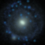
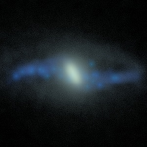
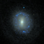
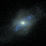
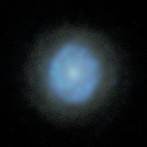
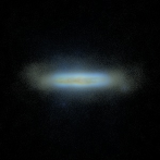
B-CS                                           B-CS⁺                                           B-MA

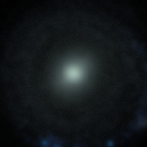
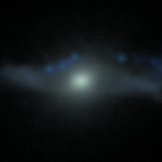
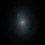
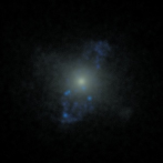
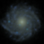
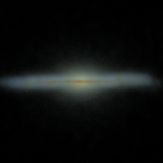
C-CS                                           C-CS⁺                                           C-MA

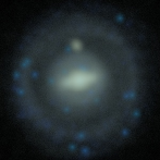
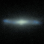
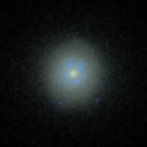
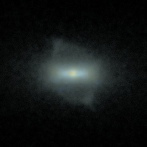
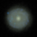
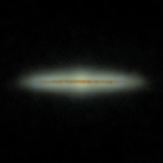
D-CS                                           D-CS⁺                                           D-MA

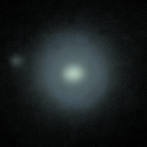
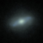
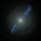
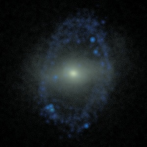
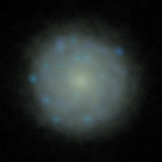
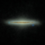
E-CS                                           E-CS⁺                                           E-MA

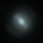
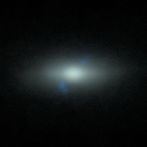
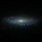
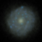
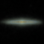
Figure 1: Multi-band ($u,r,z$) images of our fifteen galaxies, for face-on and edge-on views.

3 Creating synthetic spectra of the simulated galaxies

To derive the observables of our simulated galaxies and investigate the biases introduced in the process, we follow three approaches. First, we use different Stellar Population Synthesis (SPS) models, which provide the resulting spectrum due to the emission of the stars, as well as different informations about the stellar populations at a given metallicity and age (e.g. mass loss, ionizing photon flux, Lick indices, number of black holes and neutron stars). Second, we add a simple dust model to the prediction of the SPSs, in order to better compare the resulting spectra from those of observed galaxies. Finally, we postprocess the simulations with the radiative transfer code sunrise (Jonsson, 2006; Jonsson, Groves & Cox, 2009), which is computationally slower but more consistent with the underlying hydrodynamical simulation. This gives the full SED including stellar absorption features, nebular emission, and extinction due to dust as light travels out through the interstellar medium.

The SPS models are commonly used as a postprocessing of hydrodynamical simulations as they provides a fast and easy way to estimate the light distribution of an ensemble of stars. The use of radiative transfer codes has also been applied to hydrodynamical simulations (e.g. Governato et al. 2009; Scannapieco et al. 2010; Hayward et al. 2013; Christensen et al. 2014). This approach has the advantage that can consistently consider the distribution of dust (traced by the metals) although it also needs to introduce certain assumptions and simplifications.

In the following subsections, we describe the main aspects of these models and the assumptions that are relevant for our work, as well as discussing the main uncertainties and sources of biases in the creation of the synthetic SEDs.

3.1 Stellar population synthesis Models

We use various SPS models to create synthetic spectra of our simulated galaxies. The spectra are obtained assuming that each star particle represents a Simple Stellar Population (SSP) parametrized by the age and metallicity of the star, and normalized by the mass of the particle. In the simulations, the mass of a star particle changes with time owing to the supernova ejecta and the mass loss during the AGB phase; the mass normalization should be made with the mass of the stars at the formation time (note that this is important in order to avoid double-counting the effects of stellar mass loss). The spectrum of the galaxy is obtained by summing up the spectra of individual stars. The galaxy spectra can be convolved with given photometric bands and integrated to get the magnitude of the galaxy in the bands.

We use 5 different SPS models to obtain spectra, magnitudes and colors of our simulated galaxies, which allows us to identify systematic effects due to their varying assumptions. Although moderate, some differences between these models are expected, as uncertainties in modelling the stellar evolution still exist (e.g. different treatment of convection, rotation, mass-loss, thermal pulses during AGB evolution, close binary interaction), as well as in the empirical and theoretical stellar spectral libraries (see the reviews by Walcher et al. 2011; Conroy 2013). The main characteristics of the SPS models are described in the following, and in Table 1 we give a summary of the input parameters we chose, taken as homogeneous as possible to make the interpretation of our results more clear.

• BC03 (Bruzual & Charlot, 2003) computes, using different evolutionary tracks, the spectral evolution of stellar populations at a resolution of $3\,\mathring{A}$ FWHM in the optical and at lower resolution in the full wavelength range.

• SB99 (“STARBURST99”, Leitherer et al. 1999; Vázquez & Leitherer 2005) is a web-based platform that allows users to run customized SPS models for a wide range of IMF, isochrones, model atmospheres, ages and metallicities. The spectral resolution reaches $\sim 1\,\mathring{A}$ FWHM in the optical wavelength range for the fully theoretical spectra.

• PE (“PEGASE”, Fioc & Rocca-Volmerange 1997, 1999) uses an algorithm that can accurately follow the stellar tracks of very rapid evolutionary phases such as red super-giants or TP-AGB. The stellar library includes also cold star parameters, and a simple model for nebular emission (continuum + lines) can be added to the stellar spectrum.

• FSPS (“Flexible Stellar Population Synthesis 2.3”, Conroy, Gunn & White 2009) is a flexible SPS package that can compute spectra at resolving power $\lambda/\Delta\lambda\approx 200-500$. In addition to the choice of IMF, metallicities, ages, the user can select a variety of assumptions on Horizontal Branch (HB) morphology, blue straggler population, location of the TP-AGB phase in the HR-diagram and post-AGB phase.

• M05 (Maraston, 2005) is different from the other SPS models in the treatment of Post Main Sequence stars, namely using the Fuel Consumption theorem (Renzini & Buzzoni, 1986) to evaluate the energetics. It gives spectra at a resolution $5-10\,\mathring{A}$ in the visual region and at $20-100\,\mathring{A}$ from the NUV to the near-IR for either blue or red populations on the horizontal branch.

Table 1: Summary of the characteristics and choices of parameters for the 5 SPS models used in our work. The input stellar model in sunrise is SB99 with the same parameters.

Model	IMF	Age range (yr)	Metallicity range	Wavelength range	Stellar tracks	Stellar library
BC03	Chabrier(1)	$10^{5}-2\cdot 10^{10}$	0.0001 - 0.05	$91\,\mathring{A}-160\,\mu m$	Padova 1994	BaSeL3.1 / STELIB
M05	Kroupa(2)	$10^{3}-1.5\cdot 10^{10}$	0.0001 - 0.07	$91\,\mathring{A}-160\,\mu m$	Cassisi / Schaller	BaSeL3.1 / Lançon & Mouchine
SB99	Kroupa(2)	$10^{4}-1.5\cdot 10^{10}$	0.0004 - 0.05	$91\,\mathring{A}-160\,\mu m$	Padova 1994	Pauldrach / Hillier
PE	Kroupa(2)	$0-2\cdot 10^{10}$	0.0001 - 0.05	$91\,\mathring{A}-160\,\mu m$	Padova 1994	BaSeL3.1 / ELODIE
FSPS	Kroupa(2)	$3\cdot 10^{5}-1.5\cdot 10^{10}$	0.0002 - 0.03	$91\,\mathring{A}-10\,mm$	Padova 2007	BaSeL3.1 / Lançon & Mouchine

notes: (1) Mass range: $m=$ 0.1-100 M_⊙, $\alpha=2.3$ for $m>1$ M_⊙; (2) $\alpha=1.3$ for $m=$0.1-0.5 M_⊙, $\alpha=2.3$ for $m=$ 0.5-100 M_⊙.

3.2 Dust

Dust extinction is an important ingredient in the estimation of observables from the simulations, as in observed galaxies dust effects can be large, especially for edge-on systems. Different authors have modelled dust extinction curves of the Milky Way (e.g. Seaton, 1979; Cardelli, Clayton & Mathis, 1989), of the Large and Small Magellanic clouds (e.g. Fitzpatrick, 1986; Bouchet et al., 1985), and also of external galaxies (e.g. Silva et al., 1998; Charlot & Fall, 2000; Calzetti et al., 2000; Fischera & Dopita, 2005), which are often used to correct for dust extinction.

In our calculations of the dust-corrected magnitudes and colors, we use the model of Charlot & Fall (2000, CF00 hereafter) in the slightly different formulation given in da Cunha, Charlot & Elbaz (2008, dC08 hereafter), that consistently extend the CF00 model to include dust emission, in order to allow the interpretation of the full UV-far infrared galaxy SEDs.

CF00 is an angle-averaged time-dependent model, with extinction curve depending on the wavelength, and on the Stellar Population (SP) age. This model has been proven to work reasonably well for a wide class of galaxies, and it has been already implemented in SPS models (Bruzual & Charlot, 2003). In CF00, stars are assumed to born in “birth clouds” that disperse after a certain amount of time (see also Silva et al., 1998); the transmission function of the SP is the product of the transmission function in the birth cloud (which depends on the SP age $t$) and in the ISM:

$$T_{\lambda}^{\text{BC}}(t)=\left\{\begin{array}[]{l l}\exp\left[-(1-\mu)\,\tilde{\tau}_{V}\left(\frac{\lambda}{5500\,\text{A}}\right)^{-N_{\text{BC}}}\right]&\quad\text{for $t\leq t_{\text{BC}}$}\\ 1&\quad\text{for $t>t_{\text{BC}}$}\end{array}\right.$$

$$T_{\lambda}^{\text{ISM}}=\exp\left[-\mu\,\tilde{\tau}_{V}\left(\frac{\lambda}{5500\,\text{A}}\right)^{-N_{\text{ISM}}}\right]$$

where $t_{\text{BC}}$ is the birth cloud life-time (see CF00 and dC08 for details). The resulting attenuated luminosity $L_{\lambda}$ given the intrinsic luminosity $S_{\lambda}$ is then

$$L_{\lambda}(t)=S_{\lambda}\;T_{\lambda}^{BC}(t)T_{\lambda}^{ISM}.$$

We set the free parameters to the values given in dC08 for normal star-forming galaxies, namely: $t_{\text{BC}}=10$ Myr, $\tilde{\tau}_{V}=1.5$, $\mu=0.3$, $N_{\text{BC}}=1.3$ and $N_{\text{ISM}}=0.7$.

3.3 Radiative Transfer

To calculate the full far-UV to submillimeter SED of our simulated galaxies we use the Monte Carlo Radiative Transfer code sunrise in the post-processing phase. sunrise (Jonsson, 2006; Jonsson, Groves & Cox, 2009) is a 3D adaptive grid polychromatic Monte Carlo radiative transfer code, suited to process hydrodynamical simulations. sunrise assigns a spectrum to each star particle in the simulation, and then propagates photon “packets” from these sources through the dusty ISM using a Monte Carlo approach, assuming a constant dust-to-metals mass ratio, which we fixed to 0.4 according to Dwek (1998).

In the standard sunrise implementation, each stellar particle older than 10 Myr is assigned a spectrum corresponding to its age and metallicity from the input SPS model, in our case SB99 (see Table 1). Star particles younger than 10 Myr are assumed to be located in their birth clouds of molecular gas, and are given a modified spectrum which accounts for the effects of HII and photo-dissociation regions (PDRs). The evolution of HII regions and PDRs are described by the photo-ionization code mappings III (Groves, Dopita & Sutherland, 2004; Groves et al., 2008), which is used to calculate the propagation of the source spectrum through its nebula. The HII regions absorb effectively all ionizing radiation and are the sources of hydrogen recombination lines, as well as hot-dust emission. The only mappings III parameter not constrained by the hydrodynamical simulation is the PDR clearing timescale; in sunrise this free parameter has been changed to the time-averaged fraction of stellar cluster solid angle covered by the PDR ($f_{\text{PDR}}$), for which we use the fiducidal value of $f_{\text{PDR}}=0.2$ as in Jonsson, Groves & Cox (2009).

Dust extinction in sunrise is described by a Milky Way-like extinction curve normalized to $R_{V}=3.1$ (Cardelli, Clayton & Mathis, 1989; Draine, 2003) which includes also the $2175\AA$ bump observed in our galaxy (Czerny, 2007). Model cameras are placed around the simulated galaxies, to sample a range of viewing angles. The emergent flux is determined by the number of photons that flow from the galaxy unscattered in a given camera’s direction, as well as those scattered into the line of sight or reemitted in the infrared by dust into the camera. In the calculations presented here we use two cameras, one looking face-on and the other edge-on to the galaxy, to take into account the two extreme cases in terms of optical depth. Finally, the flux in the cameras is convolved with the bandpass filters and integrated to get the broadband images and magnitudes in the chosen photometric bands.

Fig. 2 is an example of the spectra obtained for one of our simulated galaxies, C-MA, showing in the upper panel the SB99 spectrum both without dust (pink line) and corrected with the CF00 model (blue line), as well as the dust-free stellar spectrum with sunrise (black dashed line). The lower panel shows again the sunrise stellar spectrum without dust, the full nebular+stellar spectrum without dust (red), and the full spectrum with dust from the edge-on camera (green).

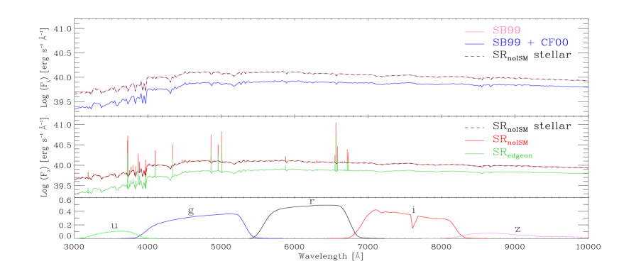
Figure 2: Examples of the SEDs obtained for one of our simulated galaxies (C-MA) using different methods, including the stellar spectrum only (SB99), the stellar spectrum and the CF00 simple dust model (SB99 + CF00), the stellar sunrise dust-free spectrum (SR_noISM stellar) and total sunrise spectra in the absence (SR_noISM) and presence of dust, for the edge-on view (SR_edgeon). The lower panel shows the SDSS filter transmission functions for the $u,g,r,i$ and $z$-bands.

3.4 Uncertainties and biases

In addition to the different assumptions of the SPS models and the treatment of dust and radiative transfer, there are a number of choices on the process of constructing the synthetic SEDs of simulated galaxies. In some cases, these constitute important sources of biases that need to be kept in mind when results are interpreted, while others do not strongly affect the final SEDs. When appropriate we will test and quantify these effects, which we describe below.

3.4.1 Aperture bias

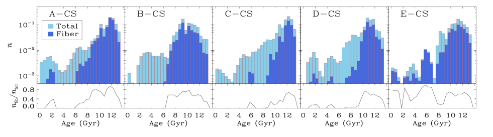
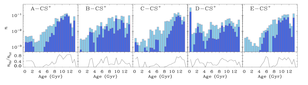
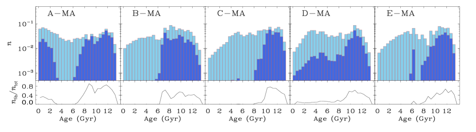
Figure 3: Number-density histograms of stellar ages for the 15 simulated galaxies, considering all star particles in the galaxies as well as only those within the fiber. For each galaxy, we also show the fraction between the number of stars within the fiber to the total number of stars in each bin, $n_{\rm fib}/n_{\rm tot}$, that we refer to as the sampling function.

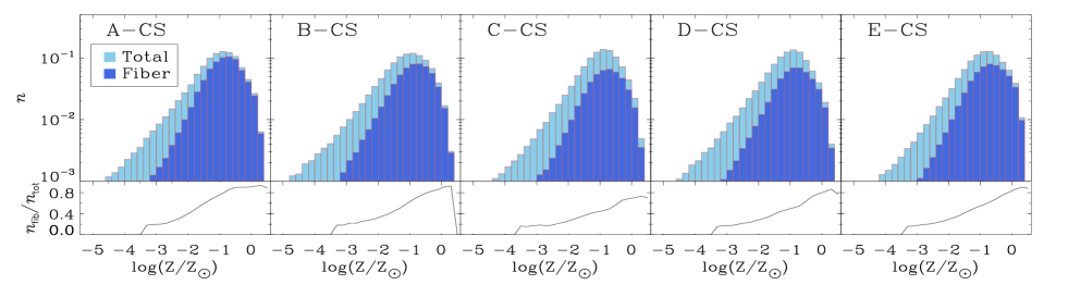
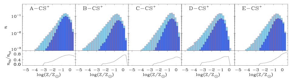
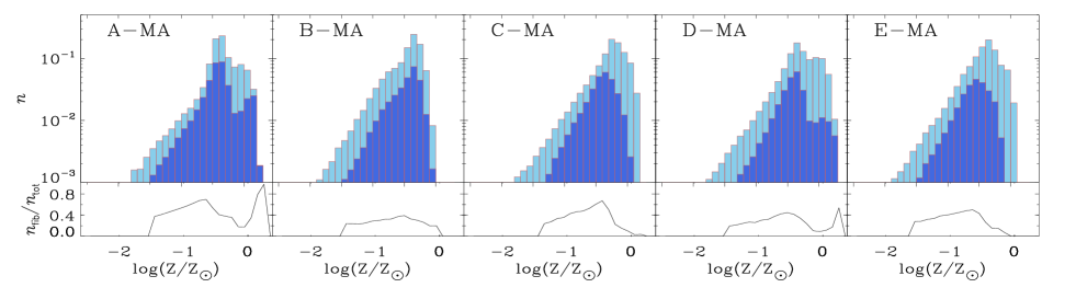
Figure 4: Number-density histograms of stellar metallicity (in solar units, assuming Z${}_{\odot}=0.02$), both for all star particles and inside the fiber field of view. For each galaxy, we also show the fraction between the number of stars within the fiber to the total number of stars in each bin, $n_{\rm fib}/n_{\rm tot}$, that we refer to as the sampling function.

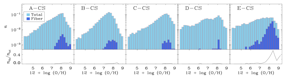
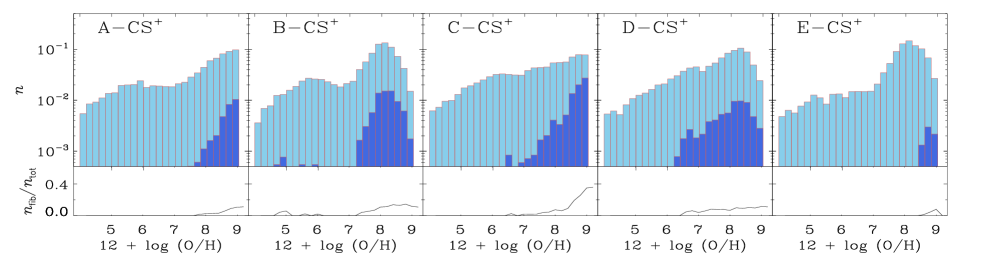
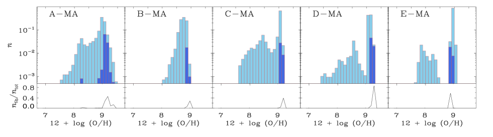
Figure 5: Number-density histograms of gas metallicity, both for all star particles and inside the fiber field of view. For each galaxy, we also show the fraction between the number of stars within the fiber to the total number of stars in each bin, $n_{\rm fib}/n_{\rm tot}$, that we refer to as the sampling function. Note the different x-range plotted for the CS/CS⁺ and MA samples.

While simulations give the full information on the phase space of particles that constitute a galaxy, observations usually have limitations related to the region that can be observed/measured, and the different techniques used to define this region in observations and simulations can introduce some systematics (Stevens et al., 2014). In SDSS, the properties derived from spectra (e.g. stellar age and metallicity, gas metallicity, SFRs) are affected by the small aperture (3” arcsec) of the SDSS spectrograph, which samples only the inner part of the target galaxies. The presence of metallicity gradients in galaxy properties and colors (Bell & de Jong, 2000; Pilkington et al., 2012; Welikala & Kneib, 2012; Sánchez et al., 2015) can therefore lead to substantial uncertainties in the observed measurements when one wants to estimate the total quantities. The implications of this bias have been discussed by several authors (Bell & de Jong, 2000; Kochanek, Pahre & Falco, 2000; Baldry et al., 2002; Gómez et al., 2003; Brinchmann et al., 2004; MacArthur et al., 2004, e.g.); in some cases methods for aperture correction which exploit the spatially-resolved color information can be used to extrapolate to global quantities (e.g. SFRs, Brinchmann et al. 2004, Salim et al. 2007).

We used our simulations to test the effects of using a single fiber in the derivation of properties such as metallicities and stellar ages, by including in the calculations both all particles in a 60x60 kpc field of view (FoV) in the face-on projection (full FoV), or only those within a small region that mimics the size sampled by the SDSS fiber spectrograph, i.e. a circular region of 4 kpc radius with the galaxy in the center observed face-on (fiber FoV), which according to the cosmology adopted in our simulations corresponds to redshift $z\sim 0.15$ for the SDSS instrument aperture. Note that we are limited to further decrease the size of the fiber field of view by having enough particles to reach a good statistical sample, in particular in the case of gas particles.

Figs. 3, 4 and 5 show the number-density histograms of stellar ages and stellar/gas metallicities for the 15 simulated galaxies, when we consider all particles in the galaxy and only those within the fiber. For each galaxy, we also show the fraction between the number of star/gas particles within the fiber to the total number of star/gas particles in each bin, $n_{\rm fib}/n_{\rm tot}$, that we refer to as the sampling function. In the case of stellar ages we find that, in general, fiber quantities preferentially sample the older populations, with sampling functions typically higher than $50\%$. In contrast, the young populations are sampled in various ways, depending on the age profile of the galaxy. In some cases, young populations are not at all sampled and will be completely missed in the calculations using particles within the fiber. It is clear, in any case, that the sampling within the fiber is not constant or even similar for all galaxies, which means that it is not possible to reliable estimate the mean stellar age of a galaxy from the fiber quantities, or even estimate the fiber bias without having additional information (e.g. importance of age/metallicity profiles) of the regions outside the fiber. We note that the relative contribution of old and young populations in a galaxy will in general reflect the relative importance of bulges and disks, but with fiber quantities this information might not be a reliable reflection of the real relative contribution of the different stellar components of a galaxy.

Similar considerations can be made in the case of the stellar metallicities, shown in Fig. 4. The metallicity distributions of the galaxies in the CS sample is broader compared to those in the MA sample, with the CS⁺ galaxies lying in between. This results from the different implementation of chemical enrichment (chemical yields increase from the CS galaxies, to CS⁺ and then to MA), chemical diffusion (only included in the MA simulations) and feedback (from weaker in CS to stronger in MA, with CS⁺ in between). In particular, the MA galaxies have more peaked distributions, and have less strong metallicity gradients (see also Aumer et al. 2013) compared to the CS and CS⁺ galaxies (see also Tissera, White & Scannapieco 2012). Unlike for the stellar ages, for the stellar metallicities we find that the sampling shows much less variation from galaxy to galaxy, as in all cases there is a preferential sampling of the more metal-rich populations.

The distributions of gas metallicities are more complex, and show important differences depending on the details of the implementation of chemical enrichment (IMF, chemical yields, etc.) and on the absence/presence of chemical diffusion, which is included only in the MA sample and leads to a much less broad distribution of gas metallicities (note the different x-scales in the lower panels). From Fig. 5, it is clear that the sampling of gas metallicities varies significantly from galaxy to galaxy. While in general there is a preferential sampling of the metal-rich regions, gas particles with intermediate metallicities can also contribute significantly to the final metallicity when fiber quantities are considered. For the MA sample, we find that, within the fiber, only a narrow range of gas metallicities are sampled, which reflects the effects of metal diffusion that tends to give a smoother metallicity distribution. In the case of the D-CS galaxy, we also find that although the metallicity distribution is broad, only a very narrow range of metallicities are sampled within the fiber. According to our findings, for estimating the gas metallicy of a galaxy it is of primary importance that the fiber bias can be quantified; otherwise it is not possible to derive the mean gas metallicity of the whole galaxy reliably.

In summary, our results show that the bias due to the fiber is in general reflected in the tendency to sample older and more metal-rich stellar populations and metal-enriched regions of the ISM, although the shape of the sampling function highly depends on the significance of gradients in ages/metallicities (which also somewhat depend on the modelling of physical processes in the simulations), affecting in particular galaxies with stronger gradients.

3.4.2 Variation of the assumed Initial Mass Function

The choice of the Initial Mass Function (IMF) can strongly bias the derivation of many observables of galaxies (see Salpeter, 1955; Miller & Scalo, 1979; Scalo, 1986; Kroupa, 2002), for example, the assumed IMF has a direct influence on the $M/L$ ratio depending on the age, composition and past star formation history (Baldry & Glazebrook, 2003; Chabrier, 2003), which in turn influences the stellar mass derivation. The IMF is measured in many environments, still there is not yet consensus on a number of important aspects, such as whether it is universal or not (e.g. Hoversten & Glazebrook, 2008; Bastian, Covey & Meyer, 2010).

We assume in general a Kroupa IMF with slope $\alpha=1.3$ for masses 0.1-0.5 $M_{\odot}$ and $\alpha=2.3$ in the mass range 0.5-100 $M_{\odot}$ when we apply the different SPS models, except in the case of BC03, where we instead use a Chabrier IMF (Table 1). The difference between these two IMFs is moderate, however, due to their very similar shape, particularly at the high-mass end (see Fig. 17 in Ellis 2008). Note that our three galaxy samples use different IMFs to calculate feedback and chemical enrichment: Salpeter (CS), Chabrier (CS⁺) and Kroupa (MA).

4 Results

In this section we describe the methods we use to derive the galaxy properties – magnitudes and colors, stellar masses, stellar ages, stellar and gas metallicities and star formation rates – from their synthetic spectra, and make a detailed comparison between results obtained with the different methods, in order to identify biases and systematics. For each property, different techniques are used in the derivation, the selection of which has been made taking into account the questions we want to answer: ($i$) what is the range of variation in observationally-derived quantities when different techniques are used, ($ii$) do they agree with the ’real’ quantity; and ($iii$) how do observational definitions of galaxy properties effect their measured values. In the case of observations, we particularly focus on the techniques employed in SDSS, which will be used in PaperII to compare simulated and observed galaxies.

In order to avoid additional biases, we always use the same field of view defined as a 60 kpc$\times$60 kpc region with the galaxy in the center both when we derive the properties directly from the simulations and from the SPS/sunrise spectra.

4.1 Magnitudes and colors

We first compare the colors and the absolute magnitudes of our simulated galaxies, in the 5 SDSS photometric bands ($u,g,r,i,z$, see Fig. 2), obtained using different methods, namely:

• BC03, SB99, FSPS, PE, M05: these refer to the magnitudes calculated by applying the five different SPS models described in Section 3.1. As explained in the previous section, for each star particle the magnitudes are obtained via a linear interpolation of the SPS tables according to its age and metallicity, normalizing with the particle mass at the formation time.

• CF00: we include dust effects to BC03 using the model of CF00/dC08 described in Section 3.2.

• SR_noISM, SR_faceon, SR_edgeon: results from the radiative transfer code sunrise as explained in Section 3.3, in the absence of dust, and for the face-on and edge-on views including dust, respectively. Note that the input SPS model for sunrise is SB99.

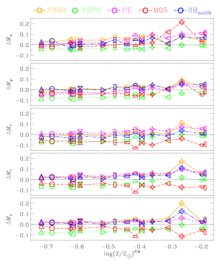
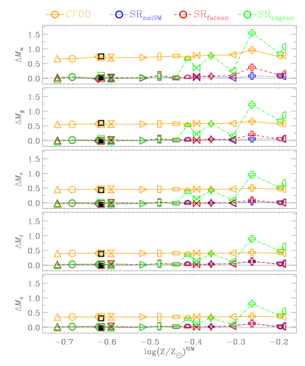
Figure 6: Difference between the absolute magnitudes of the simulated galaxies obtained using different methods and those predicted by the dust-free BC03 model, in the 5 SDSS bands and as a function of stellar metallicity. The left-hand panel shows results for dust-free models and the right-hand panel compares results of the CF00 simple dust model and of the sunrise code. The open/filled black squares are results for C-CS, when a higher dust-to-metals ratio is assumed in the sunrise calculations in edge-on and face-on views, respectively.

The left-hand panel of Fig. 6 compares the magnitudes obtained using the different SPS methods and sunrise, when we ignore the effects of dust. We show the differences with respect to BC03 as a function of the stellar metallicity of the galaxy (in solar units, assuming Z${}_{\odot}=0.02$), as systematics in SPS models are expected to increase both at low/high metallicity (as well as at younger stellar ages, e.g., Conroy, Gunn & White 2009; Conroy & Gunn 2010). The different SPS models show in general very good agreement, with magnitude differences of $\lesssim 0.1$. We detect however some systematics: models FSPS and M05 usually predict lower magnitudes (i.e. brighter galaxies) compared to BC03, while models SB99 and PE give systematically higher magnitudes than BC03. As expected, differences are somewhat larger (but still moderate) for the most metal-rich galaxies, which are also those that exhibit a higher fraction of young (ages $<10$ Myr) and intermediate (ages in the range [$0.1-2$] Gyr) stellar populations. For these ages the uncertainties in the treatment of young stars, post red-giant branch and TP-AGB phase stars are larger. The galaxy which exhibits the largest $\Delta M$ (in all bands) is A-MA, which has $\log(Z/Z_{\odot})\approx-0.26$ the most extreme SFR (Section 4.5) and the youngest mean stellar age in our sample (see next sections).

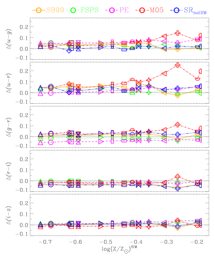
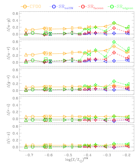
Figure 7: Difference between the colors of the simulated galaxies obtained using different methods and those predicted by the dust-free BC03 model, as a function of stellar metallicity. The left-hand panel shows results for dust-free models and the right-hand panel compares results of the CF00 dust model and of the sunrise code.

The results of SR_noISM also agree well with the rest of the models, particularly with those of SB99, as SB99 is the input SPS model of sunrise. The remaining differences are because in sunrise the spectrum for young stars is calculated with mappings III, which includes the contribution from nebular continuum and emission as well as dust absorption and IR emission that is modeled as sub-grid physics. The largest differences are found for A-MA, the galaxy with the highest number of young star particles. In fact, on one side the ionizing photons are reprocessed as nebular emission lines and continuum increasing the total flux in the optical and, on the other hand, the young particles are also more extincted due to the sub-grid treatment of dust absorption in mappings III, giving total magnitudes in general lower (brighter) by $<0.1$ mag than modelling the SED including only stellar emission.

The right-hand panel of Fig. 6 shows our results in the case of including the effects of dust, either with the CF00/dC08 correction or, more consistently, with the sunrise code. For comparison, the magnitude differences are calculated with respect to the BC03 model. When the CF00 simple dust model is included we find, as expected, fainter galaxies, with differences between $\sim 0.6-0.8$ mag for the $u$ and $g$-bands and of $\sim 0.4-0.5$ mag for $i,r$ and $z$. As the CF00 model is angle-averaged, there is no difference between face-on and edge-on views. When we consider radiative transfer effects in sunrise, we detect almost no difference if we see the galaxies face-on (SR_faceon) or if dust is ignored (SR_noISM method, included here for comparison).

As expected, larger differences are detected when galaxies are seen edge-on, as dust effects are maximal in this case. However, we find significant differences only for metal-rich galaxies, while for galaxies that are metal-poor ($\log(Z/Z_{\odot})\lesssim$-0.45) dust effects are unimportant. This is because the amount of dust in sunrise is directly proportional to the gas metallicity (galaxies with low stellar metallicity also have low gas metallicity). Observations also confirm that the dust-to-metals ratio is nearly constant over a large range of metallicities and redshifts, and dust effects are small in metal-poor galaxies (Zafar & Watson 2013, Mattsson et al. 2014). For the metal-rich galaxies, the inclusion of dust makes them fainter by factors of $\sim 0.8-1$ dex in the $u$-band and of $\sim 0.3-0.5$ dex for the $z$-band. Interestingly, for the most metal-rich galaxies the magnitudes derived from the SR_edgeon and CF00 methods are very similar. Note also that the CS⁺ galaxies have a systematically lower reddenning compared to the MA ones, even at high metallicity. This is explained by the lower amount of metals in the ISM, and therefore lower amount of dust of the galaxies in the CS⁺ sample compared to those in MA.

To explore the dependence of dust effects on metallicity for the metal-poor sample, we rerun sunrise for one galaxy (C-CS), using a higher dust-to-metals ratio of $4$ ($10$ times larger than the standard value of $0.4$ assumed in our sunrise calculations, Dwek 1998). The results are shown as open and filled squares, respectively for the edge-on and face-on views. In this case, we indeed find little effects in the case of the face-on view and larger differences in the edge-on case, with results very similar to those of CF00.

The differences in magnitudes, when different methods are applied, are translated into differences in the colors, as shown in Fig. 7. Both in the absence (left-hand panel) and in the presence (right-hand panel) of dust, differences are larger for the bluer colors ($u-g$, $u-r$ and $g-r$), and for the most metal-rich galaxies.

Our results show that applying different SPS to simulations gives visual magnitudes of galaxies with spread $0.05-0.1$ dex for metal-poor galaxies and of $0.1-0.2$ for metal-rich ones, depending on the model, with BC03 appearing as intermediate among the 5 SPS models tested. Furthermore, while for face-on galaxies or edge-on galaxies with low metallicities ($\log(Z/Z_{\odot})\lesssim-0.45$) the effects of dust can be in first approximation ignored, when galaxies are seen edge-on and have a significant amount of dust (i.e. are metal-rich), errors in the magnitudes can be up to $0.7-1.5$ dex if dust is ignored, depending on the band. This means that for edge-on galaxies, particularly metal-rich ones, reliable magnitudes will not be possible to obtain without a proper modelling of the dust extinction. Similar considerations can be made for the colors, that can not be calculated with precision better than $0.1-0.5$ dex.

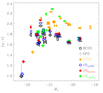
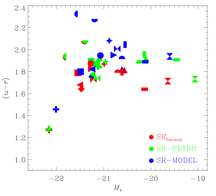
Figure 8: Color-magnitude diagram of the simulated galaxies, obtained using different methods to derive the synthetic spectra. The left-hand panel show results for the SPS, CF00 and sunrise methods and the right-hand panel compares results obtained following the SDSS techniques.

The previous figures showed the dependence of the galaxies’ magnitudes on different models and assumptions. In simulation studies, it is common to use SPS models to convert masses into luminosities, and to compare models with observational data (e.g. light profiles, magnitudes, etc). We have shown that the use of different SPS models introduces some changes in the predicted magnitudes, that are however moderate. On the other hand, when dust effects are included or a proper radiative transfer treatment is considered, larger differences might appear. In the left-hand panel of Fig. 8 we show the position of our simulated galaxies in the color-magnitude diagram; in this case in the $M_{r}$ vs ($u-r$) plane. We show the results for BC03, the spread found for all SPS models in both plotted quantities, and the results for the BC03 model with the CF00 correction. We also show results for SR_noISM, SR_faceon and SR_edgeon. These cover the commonly used ways to post-process simulation results, and allow to understand what are the possible offsets expected when more sophisticated methods are used to calculate the magnitudes. Most of our simulated galaxies have $M_{r}$ between $-22$ and $-19$, and ($u-r$) color between $\sim 1.5$ (except for A-MA) and $\sim 2.3$ (see also PaperII for a comparison with SDSS data). The A-MA galaxy lies at a different position compared to the other galaxies, particularly when dust effects are ignored or when it is included but the galaxy is seen face-on. Note that this is a young galaxy with strong emission lines, and the H$\alpha$ line falls in the $r$-filter at $z=0$. A-MA however moves photometrically closer to the other galaxies if dust extinction is included.

In observations, measuring the total magnitudes of galaxies can be plagued by different observational problems (e.g. low signal-to-noise, sky brightness, bad calibrations and sky subtraction), which affect particularly the outer part of the profiles where the S/N is lower. For this reason, definitions on how to measure the total light are used in all galaxy surveys, although they can differ substantially among authors and collaborations (e.g. Kron 1980, Blanton et al. 2001, Norberg et al. 2002). We have calculated the magnitudes and colors of our simulated galaxies following the techniques used in SDSS, in particular calculating the so-called Petrosian and Model magnitudes (Petrosian, 1976; Blanton et al., 2001; Yasuda et al., 2001; Kauffmann et al., 2003; Salim et al., 2007). These were derived from the images obtained with sunrise, including dust and in the face-on view (SR_faceon), as follows (Blanton et al., 2001):

• PETRO: we calculate the Petrosian Radius (Petrosian, 1976) in the $r$-band, and we derive the Petrosian magnitudes in all bands taking the flux inside $N_{P}=2$ Petrosian radii; as in SDSS, we assume a Petrosian Ratio $R_{P}=0.2$. Note that, in general, this method samples only part of the total flux, the fraction depending on the luminosity profile (see Graham et al. 2005 for detailed calculations).

• MODEL: in this case, each image is matched to different luminosity profiles, and the magnitudes are calculated from the profile which gives the best fit. We used the code galfit to perform the fit (Peng et al., 2010), assuming arbitrary axis ratio and position angle, and used two different profiles: Exponential and DeVaucouleur. Depending on the galaxy, one of these profiles provided the best fit: for 5 galaxies this was an exponential, for 10 a DeVaucouleur profile.

The right-hand panel of Fig. 8 compares the results obtained with the PETRO and MODEL methods to those of SR_faceon. We find in general similar values of magnitudes for the PETRO and SR_faceon methods, with PETRO magnitudes always higher (i.e. fainter) than those of SR_faceon as expected. In the case of the MODEL method, we also find fainter galaxies compared to the results of SR_faceon. In both cases, differences are lower than $0.3$ dex for 9/15 galaxies, with a maximum of $0.6$ dex for the remaining 6 systems. Colors are similar in the three models, with differences in $(u-r)$ $\lesssim 0.1-0.2$ dex. Our results show that, for our simulated galaxies the PETRO and MODEL methods can not recover the real magnitudes/colors of galaxies with a precision better than $0.2-0.3$ dex.

4.2 Stellar mass

The stellar mass of galaxies is an important proxy of how the galaxy populations evolved over cosmic time (e.g. Bell et al., 2003). In this section, we compare the stellar mass of our simulated galaxies, obtained in different ways, including the simple sum over the mass of stellar particles (as done in simulation studies) and those obtained using different post-processing techniques that mimic observations, in particular the ones used in SDSS. These are described below:

• SIM: the total mass of star particles in the simulated galaxy. We include all stars in the 60 kpc$\times$60 kpc field of view (see sec. 4), i.e., the same field of view of sunrise.

• BC03: the final mass of star particles is calculated with the BC03 model, which considers the mass lost by a stellar population since it was formed, and until the present time. The BC03 final mass of each star particle is obtained normalizing with its initial mass. The total stellar mass of the galaxy is the sum over the final masses of the star particles within the field of view.

• SED: the total stellar mass is estimated by fitting the sunrise face-on optical galaxy spectrum (SR_faceon method) over the range $3800-9000$ $\>\mathring{A}$ using the starlight code (Cid Fernandes et al., 2009) with the BC03 SPS model. The spectra include nebular emission (masked during the fit) and are dust-extincted.

• PHOTO: we fit the photometric $(u,g,r,i,z)$-band magnitudes obtained from the SR_faceon spectrum to a grid of models as updated from BC03 in 2007 (CB07, Charlot & Bruzual, priv. comm.); the grid spans a large range in galaxy star formation histories, ages and metallicities (see Walcher et al. 2008 for a description of the code). To remove the nebular contribution from the broad-band magnitudes (the fitted model considers only stellar light), we calculate the relative contribution of nebular emission within the fiber in each photometric band fitting the fiber spectrum with the starlight code, and assume that the relative contribution of nebular emission for the total galaxy is the same as in the fiber. This procedure allows one to mimic the stellar mass estimation of the Garching SDSS DR7 (which we will use in PaperII to compare simulated and observed galaxies).

• PETRO: Petrosian stellar masses are derived as in PHOTO-MASS, but using the Petrosian magnitudes (Section 4.1) as input for the fit (i.e. within 2 times the Petrosian radius). The same procedure to remove nebular emission as in PHOTO-MASS was applied in this case.

• MODEL: The same as PETRO-MASS, but using the Model magnitudes (Section 4.1).

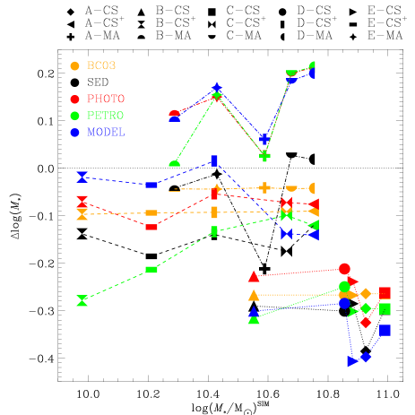
Figure 9: Comparison between different estimators of the stellar mass of galaxies, with respect to the real stellar mass, calculated as the simple sum of the mass of star particles ($M_{*}^{\rm SIM}$). Dashed and dot-dashed lines indicate simulations with a proper accounting of stellar mass loss, while dotted lines are for simulations where mass loss is not consistently followed.

In order to assess the effects of observational biases on the determination of the stellar mass of galaxies, it is important to consider the effects of mass loss of stellar particles in the simulations, as for all observationally-derived quantities, the fitting of spectra/magnitudes is done using the SPS models that include a mass loss prescription. Our 15 simulations cover the cases where mass loss is not followed, and where it is properly treated, allowing one to assess how important this effect can be. Moreover, simulations assume sometimes choices for the IMF that are different than those used in the SPS models. It is for these reasons that we calculated the stellar mass of simulated galaxies using the BC03 method additionally to the direct result of the simulation (SIM method).

In Fig. 9 we compare the stellar masses of simulated galaxies, obtained with the different methods, to the stellar mass obtained directly from the simulations (SIM). Also shown is the 1-to-1 relation (solid black line). In the lower panel, dotted, dashed and dot-dashed lines indicate respectively galaxies in the CS/CS⁺/MA samples, that differ in the treatment of mass loss of stars. We find that for galaxies where mass loss was not properly treated (CS), the stellar masses obtained with all methods are systematically lower compared to the direct result of the simulations. Furthermore, the offset is very similar for all galaxies, of the order of $0.3$ dex in log($M_{*}$). The results of the PHOTO, PETRO and MODEL methods are similar, with the former giving systematically higher stellar masses, and the latter predicting the lowest values of stellar masses.

In contrast, for galaxies in the simulations with a proper mass loss treatment (CS⁺/MA), the stellar masses obtained with the BC03 shows better agreement with the direct result (SIM), with differences up to $\sim 0.1$ dex. The SED method predicts slightly lower stellar masses, with typical differences of the order of $0.05-0.2$ dex. In the case of the PHOTO, PETRO and MODEL methods, stellar masses have some scatter up to $\sim 0.1-0.2$ dex in log($M_{*}$), and are systematically lower for CS⁺ (dashed lines) and higher for MA (dot-dashed lines) compared to the direct result of simulations.

The results of this section show that the observational estimators are able to recover the mass up to 0.1-0.2 dex in logarithmic scale, only in simulations where the mass loss of stars is consistently included. In contrast, simulations with no treatment of mass loss can still be compared with observations in a meaningful manner after a fixed correction (at least for the mass range of our sample) is applied.

4.3 Stellar ages and metallicities

The determination of stellar metallicities and ages of galaxies from observational data is usually accomplished by fitting either selected sensitive absorption line indices (e.g. Lick indices, Worthey et al. 1994, Trager et al. 1998) derived from high S/N spectra to a grid of SPS models (see Trager et al. 2000a, b; Gallazzi et al. 2005, 2006) or the full available spectrum ($\lambda$-to-$\lambda$ method, e.g. Cid Fernandes et al. 2005; Tojeiro et al. 2007, 2009; Chen et al. 2010), which also requires high quality and S/N spectra for a reliable fit. Some authors also exploit colors to estimate ages and metallicities, especially at high redshift (e.g. Lee et al., 2010; Pforr, Maraston & Tonini, 2012; Li, 2013).

In this Section, we compare the stellar ages and metallicities of the simulated galaxies obtained in different ways. In order to assess the effects of the fiber bias, for all methods we consider stars within the same field of view than in the previous section, i.e. in a projected area of $(60\text{kpc})^{2}$, and also only those within the fiber. The different methods are as follows:

• SIM: the direct result of the simulations, i.e., the mean stellar age/metallicity of a galaxy is calculated as the corresponding mass-weighted mean over the stellar particles. This requires no post-processing or additional assumptions, and is the most common way to derive ages/metallicities from simulations.

• SIM-LUM: we weight with the luminosity of stellar particles to calculate the average ages/metallicities, which more closely reflects what would be obtained in an observation; we use the $r$-band particle luminosity for stellar ages and the particles’ luminosity in all visible bands for the metallicities (both obtained with the BC03 model) to mimic the SDSS analysis (Gallazzi et al. 2005).

• SED-FIT: we fit the spectra of simulated galaxies obtained with sunrise using the starlight code (Cid Fernandes et al., 2005), selecting the best mixture of $\sim 300$ instantaneous-burst SSPs with different ages and metallicities. The fitted spectra correspond to the face-on views and include dust and nebular emission (SR_faceon method). From the fitted mixture of SSPs we calculate the mean (optical) light-weighted ages and metallicities.

• LICK-IND: the mean ages and metallicities were computed by Anna Gallazzi (priv. comm.) for a subsample of 10/15 galaxies using the method described in Gallazzi et al. (2005). The method is based on fitting five absorption features (Lick indices D$4000n$, H$\beta$, H$\delta_{A}$+H$\gamma_{A}$, [$\text{Mg}_{2}$Fe], [MgFe]) to libraries constructed with the BC03 model with different star formation history, metallicity and velocity dispersion, deriving the (optical luminosity-weighted) stellar metallicities and (r-band weighted) mean ages. As the spectra generated with SUNRISE have the resolution of the input stellar model (SB99) with spacing 20 $\mathring{A}$ (which is too low to compute meaningful absorption indices), we thus explore an alternative way to measure the Lick indices of the simulated galaxies directly from the BC03 tables, after interpolating with age and metallicity for each star particle and averaging weighting with the particle mass. However, we note that these may differ from the indices measured directly from the spectrum, as done in observations and in the model library of Gallazzi et al. used to interpret observations. For this reason, this method is not fully consistent with the one used in SDSS. We will explore this point in subsequent analysis (PaperII) with higher-resolution spectra.

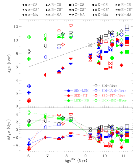
Figure 10: Difference between the mean mass-weighted stellar age in simulations and the ages calculated with the observational methods. The galaxies are sorted by increasing mean age to the right.

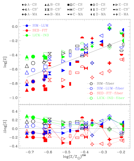
Figure 11: Difference between the mean mass-weighted stellar metallicity and the observational values, ordering the galaxies by increasing stellar metallicity to the right.

The upper panel of Fig. 10 shows the galaxies’ stellar ages obtained with the various methods described above as a function of the age obtained directly from the simulations (i.e. with the SIM method, Age^SIM), together with the 1:1 relation, while the lower panel shows the corresponding differences. Results are shown in the cases of considering all stars in the field of view and stars within the fiber.

In general, when all stars in the field of view are considered (filled symbols and solid lines), the ages obtained using the SIM-LUM and SED-FIT methods are similar, and are systematically lower than the simple average of the age of stellar particles. This results from the fact that young stellar populations emit more light than old ones, therefore have a comparatively higher weight in SIM-LUM and SED-FIT. Typical variations are of the order of $\lesssim 2$ Gyr, but the discrepancies are larger for some systems, with a maximum of about $\sim 5$ Gyr for the youngest galaxy. The estimation with the (mass-weighted) Lick indices gives systematically older ages for young galaxies (Age${}^{\rm SIM}<$ 8 Gyr) compared to SIM-LUM and SED-FIT, and slightly older ages compared to SIM, while it is in the range of the other observational estimators for the older galaxies.

Contrary to what we found for the ages estimated from all stars, in the case of the fiber quantities (open symbols and dotted lines) we find systematically higher ages compare to Age^SIM, with differences up to $\sim 4$ Gyr. Note that the differences depend sensitively on the age but also on the presence/absence of age gradients which, as shown in Fig. 3, can vary significantly from galaxy to galaxy. For old galaxies, all methods, in general, agree better with each other. We note that, for quantities within the fiber, the two sources of bias (preferential sampling of inner populations and dependence on age gradients) can lead to both positive and negative differences with respect to the direct result of the simulation. The LICK-IND method taking only particles in the fiber (LICK-IND fiber) gives in general slightly older ages compared to LICK-IND.

We also applied the three methods and calculated total and fiber quantities for the stellar metallicities. Fig. 11 shows a comparison of results. Compared to the direct result of the simulation, the SIM-LUM and SED-FIT methods give in general lower metallicities for metal-poor (old) galaxies and higher metallicities for more metal-rich (younger) ones. This is again explained by the different relative weight of old and young stars to the average metallicity (note that the spread in stellar metallicities is much smaller than that for stellar ages). Differences are however moderate, always of the order of $\pm 0.3$ dex.

For quantities within the fiber, we also find moderate differences; in this case, metallicities tend to be higher compared to total quantities, as the contribution of very low metallicity stellar populations gets smaller (Fig. 4). When we apply the LICK-IND and LICK-IND fiber methods, we find, for the low-metal sample ($\log(Z/Z_{\odot})\lesssim-0.45$), systematically higher metallicities, while for metal-rich galaxies we find better agreement with the other indicators. We detect small differences between LICK-IND and LICK-IND fiber, the latter giving in general slightly higher metallicities. It is notable that for the metal-poor galaxies, most observational methods disagree with the direct result of the simulations by an approximately constant factor, instead of scaling with the metallicity.

Our results show that in our simulations it is not possible to estimate the mean stellar age with accuracy better than $\sim 3$ Gyr, and the stellar metallicities better than $\sim 0.3$ dex, depending on the method and on the way averaged quantities are calculated. The fiber bias has a strong effect on the derived ages/metallicities, due to the preferential sampling of old and metal-rich stars; our 15 galaxies show wide variety of gradients, and therefore we find that the fiber bias when applying different methods can significantly change from galaxy to galaxy.

4.4 Gas metallicity

In this section, we compare the gas oxygen abundance of our simulated galaxies, using different estimators. Observationally, the determination of the chemical composition of the gas in galaxies is based on metallicity-sensitive emission line ratios. A number of different metallicity calibrations are used to estimate the O/H ratio in nebulae and galaxies, and comparisons among the results of various calibrations reveal large discrepancy with systematic offsets that can reach $\sim 0.7$ dex (Pilyugin 2001, see also Appendix A).

As in the previous sections, we calculate the gas chemical composition following the most common methods from simulations and observations, and, when appropriate, considering all gas particles and only those within the fiber (labelled as “fiber”). When we use (face-on) sunrise spectra for the calculation (T04, KK04, $T_{e}$), we first Balmer-correct the emission line ratios for dust extinction using the Calzetti law (Calzetti, Kinney & Storchi-Bergmann, 1994). The methods are described in the following.

• SIM: the gas metallicity of a galaxy is calculated as the mean (O/H) of gas particles, weighted by their mass.

• HII: is the mean mass-weighted O/H of gas particles, but only considering particles around stars younger than 20 Myr and inside 1 kpc radius. In this way, we mimic the preferential bias to young stellar populations in nebulae-based measurements. Note that although the HII regions have sizes which can vary in a wide range of $0.1-200$ pc from ultra-compact to giant extragalactic HII regions, we are limited to define smaller sizes of the HII regions by the resolution of the simulations, which is of the order of $\sim 1$ kpc.

• T04 (Tremonti et al., 2004): the gas metallicity is computed using the calibration of the $R_{23}$-upper branch given in Tremonti et al. (2004). According to Kewley & Ellison (2008) we use [NII]/[OII] to remove the degeneracy in the $R_{23}$-metallicity relation, and we define the upper branch as $\text{Log ([NII]/[OII])}\geq-1.2$ (see also Appendix A).

• KK04 (Kobulnicky & Kewley, 2004): is a widely used metallicity calibration, based on an iterative method that allows to solve both the oxygen abundance and ionization parameter using the $O_{32}$ and $R_{23}$ line ratios.

• $\mathbf{T_{e}}$: the electron-temperature calibration (also referred to as “direct” method) is based on the ratio between the auroral line [OIII] $\lambda 4363$ and [OIII] $\lambda 4959,5007$; it is commonly used to determine gas metallicities when the weak auroral line can be detected. Here we follow the procedure outlined in Izotov et al. (2006).

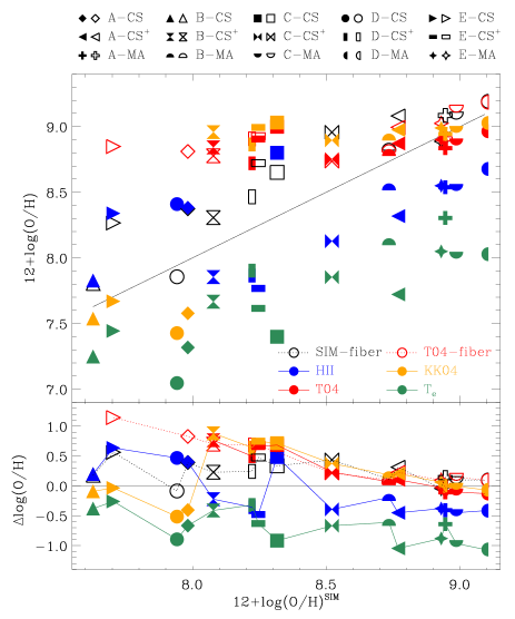
Figure 12: Comparison between the different estimators for the the galaxies’ oxygen gas metallicities, as a function of that obtained with the SIM method. For reference, in the upper panel we include the 1:1 relation as a solid line. As explained in the text, T04 calibration is valid only for a subsample of the galaxies.

Fig. 12 shows our results for the oxygen abundances of the simulated galaxies obtained using the different methods. We show results as a function of the real gas metallicity, i.e. 12+log(O/H)^SIM, the differences are also calculated with respect to this estimator. As expected, the metallicities predicted using the SIM-fiber and T04-fiber methods are systematically higher compared to SIM as the most metal-enriched regions in the bulge are preferentially sampled in these cases. This happens however only for the metal-poor galaxies, while for the metal-rich ones these estimators agree very well. Note that, in our simulations, the galaxies with low/moderate metal content (CS and CS⁺ samples) are also the ones with stronger metallicity gradients, while galaxies in the MA sample do not show significant metallicity gradients, masking a possible bias due to preferential sampling (see also Fig. 5). The HII estimator, which samples the gas near young star particles, shows $\pm 0.5$ dex scatter around the SIM value, in general higher for the galaxies with $12+$log(O/H)$\lesssim$ 8.3 and lower for the more oxygen-rich ones.

The gas metallicities obtained with the emission-line calibration of T04 are systematically higher, with large discrepancies only for galaxies with low metal content. However, note that only for 11/15 galaxies this calculation is possible. Also for the KK04 method, we find good agreement with SIM for the metal-rich systems, with some offsets for metal-poor galaxies (i.e. $12+\log(\text{O/H})\lesssim 8.3$).

The largest discrepancies in gas metallicities, both with respect to the real value and to the other observational estimators, are found for the $T_{e}$ method, which gives the lowest metallicity values. Unlike the other methods, the systematically lower metallicities are found even for the most metal rich galaxies where the rest of the methods agree well. The largest differences are of the order of $\sim 1$ dex, and only a weak trend with the metallicity is detected.

It is worth noting that the emission line intensities in the spectra calculated from sunrise rely on the mappings III photoionization code. The line ratios are then affected by uncertainties, assumptions and approximations in the model that describe the photodissociation regions, e.g. on-the-spot approximation (Stasińska, 2002, 2007), assumptions on the geometry of the nebula, dust grain composition, shocks, etc. (Groves, Dopita & Sutherland, 2004), which will in turn affect the derivation of the gas metallicities. In any case, our results show that wide differences in metallicity can appear due to the use of various calibrations even on the same spectrum modeled with a given photoionization code.

In summary, our analysis shows that the fiber bias has a strong effect on the mean gas metallicity of galaxies, particularly for metal-poor systems and for systems with strong metallicity gradients, with metallicities systematically higher, up to $\sim 1$ dex, compared to the total mean metallicities. Deriving metallicities from the emission-line calibrations shows also large offsets, that can reach $0.5-0.8$ dex compared to the value in the simulations, but in this case, the results are more diverse, with both positive and negative differences. Finally, the calibration based on electron temperature predicts systematically lower metallicities, by $0.7-1$ dex, compared to the rest of the methods and to the metallicities derived directly from the simulations.

4.5 Star formation rate

In observations, the SFR of galaxies is estimated using different methods at different redshifts, e.g. the luminosity of the H$\alpha$ line, of the $[OII]\lambda 3727$ line and the UV continuum for low, intermediate and high redshifts, respectively. Each SFR indicator is affected by theoretical biases and observational uncertainties (e.g. different timescale, sparse wavelength sampling, contribution from old stars, AGN contamination) which can influence the final SFR value (Calzetti, 2008). Furthermore, the use of different SFR proxies at different redshifts may introduce systematic errors that can bias the comparison between simulations and observations (Rosa-González, Terlevich & Terlevich, 2002).

In this section, we calculate the SFRs of our simulated galaxies with different methods. We use the calibrations given in Kennicutt (1998), applying the correction factor $f_{\rm IMF}=1.5$ (Calzetti et al., 2009) to account for the use of a different IMF (Kennicutt 1998 assumes a Salpeter IMF while we assume a Kroupa IMF in sunrise and Chabrier in BC03). We note that, in SDSS, the fiber-derived SFRs (Brinchmann et al., 2004) are corrected to total SFR with the Salim et al. (2007) method. For this reason, we use the full face-on spectra obtained with sunrise, dust-corrected with the Calzetti law, to derive SFRs, instead of the spectra within the fiber. The various methods to derive SFRs are described below.

• SIM: the real SFR extracted directly from the simulations (stellar mass formed over time interval), averaged over the past 0.2 Gyr.

• BC03: we convert the rate of ionizing photons calculated with BC03 into SFR:

  $${\rm SFR}({\rm M}_{\odot}\,{\rm yr}^{-1})=1.08\,f_{\rm IMF}^{-1}\times 10^{-53}Q(H^{0})\,({\rm s}^{-1}).$$

• H$\alpha$: we extract the H$\alpha$-luminosity from the sunrise spectrum and convert into SFR according to:

  $${\rm SFR}({\rm M}_{\odot}\,{\rm yr}^{-1})=7.9\,f_{\rm IMF}^{-1}\times 10^{-42}L(H\alpha)\,({\rm erg\ s}^{-1}).$$

• UV: we calculate the flux from sunrise spectra of the nearly-flat region between $1500-2800\>\mathring{A}$ and calculate the SFR as:

  $${\rm SFR}({\rm M}_{\odot}\,{\rm yr}^{-1})=1.4\,f_{\rm IMF}^{-1}\times 10^{-28}L_{\nu}\,({\rm erg\ s}^{-1}{\rm Hz^{-1}}).$$

• [OII]: we estimate the SFR using the luminosity of the forbidden-line doublet [OII]$\lambda 3726,3729$ in sunrise:

  $${\rm SFR}({\rm M}_{\odot}\,{\rm yr}^{-1})=1.4\,f_{\rm IMF}^{-1}\times 10^{-41}L({\rm OII})\,({\rm erg}\ s^{-1}).$$

• FIR: the SFR is estimated from the sunrise FIR luminosity integrated over the range $8-1000\>\mu\text{m}$ as:

  $${\rm SFR}({\rm M}_{\odot}\,{\rm yr}^{-1})=4.5\,f_{\rm IMF}^{-1}\times 10^{-44}L_{FIR}\,({\rm erg}\ s^{-1}).$$

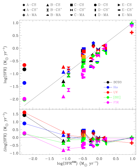
Figure 13: Comparison between the SFRs obtained using various methods as a function of the real SFR of the simulation (method SIM). In the upper box, we also include the 1:1 relation for reference.

All observational methods are sensitive to the emission from young massive stars, although the UV indicator has 10 times longer timescale ($\sim 100$ Myr), because massive stars stay luminous for longer time in the UV with small production of ionizing photons (Calzetti, 2008).

Fig. 13 shows the differences between the SFR obtained with the different estimators and that obtained directly from the simulations (SFR^SIM). Except for the galaxy with the lowest SFR, the SFRs obtained with BC03, H_α and UV methods agree well, with differences of $\lesssim 0.2-0.4$ dex in logarithmic scale with respect to the real SFR of the simulations. Note that BC03 and H_α are based on the same method (conversion of the number of ionizing photons into SFR), but use two different models.

The other observational indicators ([OII] and FIR) predict in general lower SFRs compared to SFR^SIM, with maximum differences of about 1 dex. In particular, the [OII]-SFRs of metal-poor galaxies are significantly lower than SFR^SIM, by $\sim 0.5$ dex. Note that the [OII] line intensity and [OII]/H$\alpha$ ratio strongly depend on the metallicity (Kewley, Geller & Jansen, 2004) and has been calibrated by Kennicutt (1998) for around-solar metallicity; this calibration is not accurate for the metal-poor galaxies of our sample. Also in the case of the SFR obtained with the FIR method differences are expected, as the Kennicutt (1998) calibration is valid only for dusty metal-rich starburst galaxies (note that calibrations that follow both dust-obscured and unobscured star formation can be found in the literature, see Calzetti 2008); for the metal-poor sample, since the amount of dust in sunrise is proportional to the metallicity, we have only small dust absorption (Sec. 4.4) and reemission in the infrared (see also Hayward et al. 2014). To further investigate this effect, we plot in Fig. 13 the result obtained using the FIR method of one of our metal-poor galaxies (C-CS, orange square) where the assumed dust-to-metal ratio in sunrise was increased 10 times (as in Section 4.1). In this case, the SFR raises by $\sim 0.6$ dex, although it is still moderately lower compared to the results of the other estimators.

Finally, note that SFRs derived observationally and in simulations assume different timescales, of about $10-100$ Myr for the former compared to $0.2-0.5$ Gyr for the latter. This can result in significant discrepancies among the two estimations if we are in the presence of recent starbursts. In our sample, however, we observe such a systematic difference only in the galaxy with the lowest SFR (D-CS).

The results of this section show that the SFRs indicators exhibit differences of $\lesssim 0.4$ dex in log(SFR), which are caused both by the difference in methods and the different characteristic time-scales to which the methods are sensitive. The $H_{\alpha}$ and UV methods predict similar SFRs compared to the direct results of the simulations, except for the galaxy with the lowest SFR. For galaxies with low metallicities the [OII] method gives systematically lower SFRs, with absolute differences lower than $0.5$ in logarithmic scale. For the FIR method the differences are larger in metal-poor galaxies, with SFRs systematically lower by $0.5-1$ dex in log(SFR), while the FIR estimation agrees with the SFR of the simulations up to $0.1-0.2$ dex for metal-rich galaxies.

5 Discussion and conclusions

We have used a set of 15 simulated galaxies, of similar mass to the Milky Way, to study biases and systematics in the derivation of observables, and in the comparison between them and observational data. The aim of this study is twofold; first, help simulators to be aware of systematics and be able to reliably judge the agreement between simulated and observed galaxies and, second, help observers to interpret observational results by being able to better quantify the differences between the observationally-obtained galaxy properties and the real ones (that are known in the simulations).

Our simulations comprise 15 galaxies with a variety of merger, formation and accretion histories, which results in a variety of final morphologies, star formation rates, gas fractions and metallicities. As these properties somewhat depend on the modelling of feedback, the same 5 galaxies were simulated using three different models for chemical/energy feedback; the strength of feedback and the amount of chemical yields varies from moderate to strong. For moderate feedback we find galaxies that are more metal-poor and form their stars earlier, while for strong feedback we find younger galaxies with a higher metal content. This diversity, typical of real galaxies, makes the sample ideal to test biases and systematics in the derivation of the synthetic spectra, and to study the dependence of such effects on galaxy properties (with the caveat that with our sample we do not represent the more metal rich galaxies observed).

For our study we have computed the synthetic spectra of the simulated galaxies at $z=0$, as at low-redshift many databases of galaxy properties derived from large galaxy surveys (e.g. SDSS, 2dFGRS and 6dFGS) are available. For this purpose, we followed three different approaches: ($i$) Stellar Population Synthesis (SPS) models, which give the spectra coming from stars; ($ii$) SPS models including dust extinction with a simple recipe; and ($iii$) a full radiative transfer calculation that gives the spectra including stellar and nebular emission, as well as the effects of dust which are parametrized using the metallicity of the interstellar medium. We have used the synthetic spectra to derive the observables (magnitudes/colors, stellar masses and ages, stellar/gas metallicities and star formation rates) in various ways, as to mimic real observations, and we have compared the results with the direct outputs of the simulations, i.e. the real galaxy properties.

Biases and systematics appear at various stages in the process of obtaining the observables from the simulations, due to:

- assumptions and parameters of SPS models,

- dust/radiative transfer/projection effects,

- weighting with the mass instead of luminosity for mean quantities,

- observational biases, such as extrapolation to external regions of galaxies where no spectral/photometric data are available (e.g. fiber bias, Petrosian/Model magnitudes),

- different parametrization of the star formation history and dust extinction when quantities are derived fitting a pre-constructed grid of models,

- in the particular case of gas metallicities and SFRs, the use of different calibrations.

We tested the effects of such biases on the magnitudes and colors of simulated galaxies, their stellar masses, ages, stellar/gas metallicities and star formation rates. Our results can be summarized as follows:

• Magnitudes

  - The galaxies’ magnitudes in the (u,g,r,i,z) SDSS bands derived from the five different SPS models used in our work show good agreement, with differences lower than $0.1$ dex. Differences are larger for the most metal-rich galaxies, which also have a higher contribution of young and intermediate age stars, for which model uncertainties are the largest.

  - Dust effects can be important if galaxies are seen edge-on. A simple angle-averaged dust model predicts galaxies that are $\sim 0.4-0.8$ dex fainter compared to the no-dust case. If full radiative transfer is considered, where dust is traced by the metals, edge-on galaxies appear in general $\sim 0.3-1$ dex fainter, but only if these are relatively metal-rich.

  - Estimating the magnitudes using a more observational approach (as for instance the Petrosian and Model magnitudes of SDSS) exhibits some differences compared to the real magnitudes of the simulated galaxies, with offsets $\sim 0.2-0.3$ dex for $60\%$ of the systems and up to $0.6$ dex for the remaining $40\%$.

• Stellar masses:

  When observational techniques are applied to the simulated galaxies to estimate their stellar masses, the results vary depending on the treatment of mass loss in the simulations:

  - If mass loss includes only SNe (which is a small effect), all observational estimators give systematically lower stellar masses compared to the direct result of the simulation, as the fitted models include the full mass loss of Stellar Populations at each stage of evolution. The offset is similar for all galaxies, of about a factor $0.3$ in log($M_{*}$) or, equivalently, of 50$\%$ in $M_{*}$.

  - If mass loss is properly treated in the simulations (e.g. adding AGB stars), the observational techniques recover the real stellar masses with differences $0.1-0.2$ dex in log($M_{*}$).

• Stellar ages:

  - If stellar ages are estimated mimicking observational techniques weighting with the luminosity (but ignoring the fiber bias), galaxies appear younger, typically by $\sim 2$ Gyr, compared to the direct result of simulations (mean age of stellar particles). Some galaxies exhibit larger differences, up to a maximum of $5$ Gyr; among them, we find both very young and very old galaxies.

  - If only stars in the nuclear part of galaxies are included (as to mimic single-fiber surveys such as SDSS), the observationally-estimated galaxy ages are in general higher compared to the direct result of the simulations with differences of about $2-4$ Gyr for young systems and of $\lesssim 1$ Gyr for old ones. However, the results depend sensitively on the particular properties of galaxies, namely the presence of significant/insignificant age gradients and the resulting preferential sampling of old stars within the fiber.

• Stellar metallicities:

  - Observationally-estimated stellar metallicities (ignoring the fiber bias) are in general lower compared to the direct result of the simulations, in particular if galaxies are metal-poor, with differences up to $-0.3$ in logarithmic scale. For more metal-rich systems, differences are similar in absolute value, but can vary from positive to negative. The differences in the behaviour of metal-rich/metal-poor galaxies originates in the different weight of old/metal-poor and young/metal-rich stars in the different methods, in particular depending on the way the mean metallicity is calculated (mass/luminosity-weighted).

  - If only stars within the fiber are considered, stellar metallicities tend to be higher compared to the direct result of the simulations with typical differences of $\sim 0.1-0.3$ dex and no strong dependence with the real stellar metallicity.

• Gas metallicities:

  - Deriving gas metallicities using different emission-line calibrations show large spread in the resulting metallicity values, up to $0.5-0.8$ dex. In general, metallicities lower than the real value are predicted for very metal-poor systems, while for more metal-rich galaxies they show a better agreement. Significant differences are found when the calibration based on electron temperature is used; in this case the derived metallicities are systematically lower by differences of the order of $0.7-1$ dex.

  - Gas metallicities are systematically higher than the direct result of simulations when the fiber bias is included, due to a preferential sampling of metal-rich regions in the galaxy. Differences can be up to $1$ dex for the most metal-poor galaxies, while the for metal-rich sample differences are always smaller than $0.1$ dex.

• Star formation rates:

  - Observationally-derived SFRs using different indicators present in general offsets of the order of $\pm 0.4$ dex in log(SFR), mainly due to the differences in methods and time-scales to which they are sensitive. The largest differences are found for the estimations based on the FIR, which gives systematically lower SFR values up to $1$ dex in logarithmic scale for the metal-poor galaxies.

In summary, we have shown that it is important to properly take into account different observational biases when galaxy observations are interpreted and linked to different underlying physical processes. Furthermore, a meaningful comparison between observations and simulations of galaxies requires a good understanding of the systematics; if this is not considered it is not possible to properly judge agreement/disagreement between simulations and observations, and to decide which of the physical processes included in the simulations are more relevant in the context of the formation and evolution of galaxies in a cosmological context.

In a companion paper (Guidi et al., in prep.), we compare the properties of our simulated galaxies to observations of the SDSS survey, in order to gain more insight in their agreement/disagreement in relation to the treatment of feedback, star formation, mass loss and chemical enrichment in the simulations. We also quantity differences from the observationally-derived quantities and the direct result of the simulations to provide the relevant scalings and error bars for a meaningful comparison, in the case of the different galaxy properties.

Finally, we note that other possible sources of biases and systematics have not been explored here, e.g. related to the inability to resolve the typical height of gaseous discs (which could affect the comparison between face-on and edge-on projections). Moreover, how well the simulated galaxies reproduce the observed sizes/concentrations/luminosity profiles can affect our findings related to the fiber bias and Petrosian/Model Magnitudes (although in previous papers we have shown that our models produce galaxies in broad agreement with observational results, e.g. Scannapieco et al. 2010, Scannapieco et al. 2012, Aumer et al. 2013). We hope that our work encourages other researches to explore all these issues, as well as we will continue to test systematics/biases in further analysis.

Appendix A Gas metallicity calibrations

The observational derivation of the gas metallicity of galaxies requires a calibration of emission lines to recover the (O/H) ratio; different ones are used in various observational campaigns (e.g Zaritsky, Kennicutt & Huchra 1994; Kobulnicky & Kewley 2004; Kewley et al. 2002; Pettini & Pagel 2004). Previous work has already shown that large discrepancies, as large as $\sim 0.7$ dex, arise when different calibrations are used (Pilyugin, 2001). The calibrations can be broadly classified as empirical (further subdivided into “direct” and “statistical”) and theoretical. The former derives metal abundances directly from electron temperature-sensitive lines or relations between temperature-estimated metallicities and strong emission lines, while the latter relies on photoionization models to calibrate the metallicity indicators (see the reviews by Ferland 2003; Stasińska 2007 and Kewley & Ellison 2008).

In general, theoretical calibrations give, for a given galaxy, a higher metallicity compared to electron temperature-based estimators (Liang et al., 2006; Kewley & Ellison, 2008). The causes of these discrepancies are still unclear, although some authors conjecture either problems in the photoionization models (Kennicutt, Bresolin & Garnett, 2003), or temperature gradient fluctuations in the nebulae (Stasińska, 2005, 2007; Bresolin, 2008). The effects of these disagreements can also bias the determination of the shape and the zero point in the mass-metallicity relation (Andrews & Martini, 2013).

Fig. 14 presents a comparison between the oxygen abundance of our simulated galaxies assuming various calibrations, that we summarize in Table 2. All results are derived after Balmer-correcting the emission line ratios for dust extinction using the Calzetti law (Calzetti, Kinney & Storchi-Bergmann, 1994). Some calibrations have limited ranges of validity, and here we only show results for galaxies that satisfy these conditions (see Kewley & Ellison 2008 for details).

Table 2: Main characteristics of the different metallicity calibrations (see Kewley & Ellison 2008 for more details).

Method	Class	Reference
T04	theoretical	Tremonti et al. (2004)
KK04	theoretical	Kobulnicky & Kewley (2004)
$T_{e}$	direct	Izotov et al. (2006)
Z94	theoretical	Zaritsky, Kennicutt & Huchra (1994)
KD02	theoretical	Kewley et al. (2002)
M91	theoretical	McGaugh (1991)
D02	combined	Denicoló, Terlevich & Terlevich (2002)
PP04	empirical	Pettini & Pagel (2004)
PP04(O3N2)	empirical	Pettini & Pagel (2004)
P05	empirical	Pilyugin, Vílchez & Thuan (2010)

It is clear that the metallicities for the various emission-line calibrations show larger differences, up to $\sim\pm 1$ dex. The use of different calibrations is certainly a source of concern, although in general the discrepancies are similar for all galaxies regardless their metallicities, although variations are smaller for the more metal-rich galaxies. In particular, the calibration based on electron temperature is in general lower than the others (see Sec. 4.4), manifesting itself as a clear offset, particularly for galaxies with (direct) metallicities higher than $12+\log(O/H)\sim 8.2$. On the other hand, T04 and Z94 give the highest metallicity values, with the other calibrations lying in between. For the most metal-rich galaxies, a number of indicators agree relatively well, particularly KK04, KD02, M91, and even T04 and Z94, with a small spread of $\sim 0.1-0.2$ dex (note that all of these are theoretical calibrations). For the most metal-poor galaxies, we also find that various of the calibrations agree relatively well with each other, still with variations of $\pm 0.5$ dex.

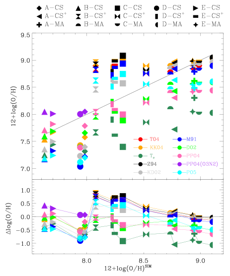
Figure 14: Comparison of the gas metallicity of simulated galaxies using different calibrations, as a function of the direct result of the simulation.

References

- Abadi et al. (2003) Abadi M. G., Navarro J. F., Steinmetz M., Eke V. R., 2003, ApJ, 591, 499
- Abazajian et al. (2003) Abazajian K., Adelman-McCarthy J. K., Agüeros M. A., et al., 2003, AJ, 126, 2081
- Andrews & Martini (2013) Andrews B. H., Martini P., 2013, ApJ, 765, 140
- Aumer et al. (2013) Aumer M., White S. D. M., Naab T., Scannapieco C., 2013, MNRAS, 434, 3142
- Baldry & Glazebrook (2003) Baldry I. K., Glazebrook K., 2003, ApJ, 593, 258
- Baldry et al. (2002) Baldry I. K., Glazebrook K., Baugh C. M., et al., 2002, ApJ, 569, 582
- Bastian, Covey & Meyer (2010) Bastian N., Covey K. R., Meyer M. R., 2010, ARA&A, 48, 339
- Bell & de Jong (2000) Bell E. F., de Jong R. S., 2000, MNRAS, 312, 497
- Bell et al. (2003) Bell E. F., McIntosh D. H., Katz N., Weinberg M. D., 2003, ApJS, 149, 289
- Blanton et al. (2001) Blanton M. R., Dalcanton J., Eisenstein D., Loveday, 2001, AJ, 121, 2358
- Bouchet et al. (1985) Bouchet P., Lequeux J., Maurice E., Prevot L., Prevot-Burnichon M. L., 1985, A&A, 149, 330
- Bresolin (2008) Bresolin F., 2008, in The Metal-Rich Universe, Israelian G., Meynet G., eds., p. 155
- Brinchmann et al. (2004) Brinchmann J., Charlot S., White S. D. M., Tremonti C., Kauffmann G., Heckman T., Brinkmann J., 2004, MNRAS, 351, 1151
- Bruzual & Charlot (2003) Bruzual G., Charlot S., 2003, MNRAS, 344, 1000
- Calzetti (2008) Calzetti D., 2008, in Astronomical Society of the Pacific Conference Series, Vol. 390, Pathways Through an Eclectic Universe, Knapen J. H., Mahoney T. J., Vazdekis A., eds., p. 121
- Calzetti et al. (2000) Calzetti D., Armus L., Bohlin R. C., Kinney A. L., Koornneef J., Storchi-Bergmann T., 2000, ApJ, 533, 682
- Calzetti, Kinney & Storchi-Bergmann (1994) Calzetti D., Kinney A. L., Storchi-Bergmann T., 1994, ApJ, 429, 582
- Calzetti et al. (2009) Calzetti D., Sheth K., Churchwell E., Jackson J., 2009, in The Evolving ISM in the Milky Way and Nearby Galaxies, p. 8
- Cardelli, Clayton & Mathis (1989) Cardelli J. A., Clayton G. C., Mathis J. S., 1989, ApJ, 345, 245
- Chabrier (2003) Chabrier G., 2003, PASP, 115, 763
- Charlot & Fall (2000) Charlot S., Fall S. M., 2000, ApJ, 539, 718
- Chen et al. (2010) Chen X. Y., Liang Y. C., Hammer F., Prugniel P., Zhong G. H., Rodrigues M., Zhao Y. H., Flores H., 2010, A&A, 515, A101
- Christensen et al. (2014) Christensen C. R., Brooks A. M., Fisher D. B., Governato F., McCleary J., Quinn T. R., Shen S., Wadsley J., 2014, MNRAS, 440, L51
- Cid Fernandes et al. (2005) Cid Fernandes R., Mateus A., Sodré L., Stasińska G., Gomes J. M., 2005, MNRAS, 358, 363
- Cid Fernandes et al. (2009) Cid Fernandes R. et al., 2009, in Revista Mexicana de Astronomia y Astrofisica Conference Series, Vol. 35, Revista Mexicana de Astronomia y Astrofisica Conference Series, pp. 127–132
- Colless (1999) Colless M., 1999, Royal Society of London Philosophical Transactions Series A, 357, 105
- Conroy (2013) Conroy C., 2013, ARA&A, 51, 393
- Conroy & Gunn (2010) Conroy C., Gunn J. E., 2010, ApJ, 712, 833
- Conroy, Gunn & White (2009) Conroy C., Gunn J. E., White M., 2009, ApJ, 699, 486
- Creasey et al. (2015) Creasey P., Scannapieco C., Nuza S. E., Yepes G., Gottlöber S., Steinmetz M., 2015, ApJ, 800, L4
- Czerny (2007) Czerny B., 2007, in Astronomical Society of the Pacific Conference Series, Vol. 373, The Central Engine of Active Galactic Nuclei, Ho L. C., Wang J.-W., eds., p. 586
- da Cunha, Charlot & Elbaz (2008) da Cunha E., Charlot S., Elbaz D., 2008, MNRAS, 388, 1595
- Denicoló, Terlevich & Terlevich (2002) Denicoló G., Terlevich R., Terlevich E., 2002, MNRAS, 330, 69
- Draine (2003) Draine B. T., 2003, ApJ, 598, 1017
- Dwek (1998) Dwek E., 1998, ApJ, 501, 643
- Ellis (2008) Ellis R. S., 2008, Observations of the High Redshift Universe, Loeb, A. and Ferrara, A. and Ellis, R. S., pp. 259–364
- Fabian (2012) Fabian A. C., 2012, ARA&A, 50, 455
- Ferland (2003) Ferland G. J., 2003, ARA&A, 41, 517
- Fioc & Rocca-Volmerange (1997) Fioc M., Rocca-Volmerange B., 1997, A&A, 326, 950
- Fioc & Rocca-Volmerange (1999) Fioc M., Rocca-Volmerange B., 1999, arXiv:astro-ph/9912179
- Fischera & Dopita (2005) Fischera J., Dopita M., 2005, ApJ, 619, 340
- Fitzpatrick (1986) Fitzpatrick E. L., 1986, AJ, 92, 1068
- Gallazzi et al. (2006) Gallazzi A., Charlot S., Brinchmann J., White S. D. M., 2006, MNRAS, 370, 1106
- Gallazzi et al. (2005) Gallazzi A., Charlot S., Brinchmann J., White S. D. M., Tremonti C. A., 2005, MNRAS, 362, 41
- Garnett & Shields (1987) Garnett D. R., Shields G. A., 1987, ApJ, 317, 82
- Gómez et al. (2003) Gómez P. L. et al., 2003, ApJ, 584, 210
- Governato et al. (2009) Governato F. et al., 2009, MNRAS, 398, 312
- Governato et al. (2007) Governato F., Willman B., Mayer L., Brooks A., Stinson G., Valenzuela O., Wadsley J., Quinn T., 2007, MNRAS, 374, 1479
- Graham et al. (2005) Graham A. W., Driver S. P., Petrosian V., Conselice C. J., Bershady M. A., Crawford S. M., Goto T., 2005, AJ, 130, 1535
- Groves et al. (2008) Groves B., Dopita M. A., Sutherland R. S., Kewley L. J., Fischera J., Leitherer C., Brandl B., van Breugel W., 2008, ApJS, 176, 438
- Groves, Dopita & Sutherland (2004) Groves B. A., Dopita M. A., Sutherland R. S., 2004, ApJS, 153, 9
- Hayward et al. (2014) Hayward C. C. et al., 2014, MNRAS, 445, 1598
- Hayward et al. (2013) Hayward C. C., Narayanan D., Kereš D., Jonsson P., Hopkins P. F., Cox T. J., Hernquist L., 2013, MNRAS, 428, 2529
- Hoversten & Glazebrook (2008) Hoversten E. A., Glazebrook K., 2008, ApJ, 675, 163
- Izotov et al. (2006) Izotov Y. I., Stasińska G., Meynet G., Guseva N. G., Thuan T. X., 2006, A&A, 448, 955
- Jonsson (2006) Jonsson P., 2006, MNRAS, 372, 2
- Jonsson, Groves & Cox (2009) Jonsson P., Groves B., Cox T. J., 2009, arXiv:0906.2156
- Kauffmann et al. (2003) Kauffmann G., Heckman T. M., White S. D. M., Charlot, 2003, MNRAS, 341, 33
- Kennicutt (1998) Kennicutt, Jr. R. C., 1998, ARA&A, 36, 189
- Kennicutt, Bresolin & Garnett (2003) Kennicutt, Jr. R. C., Bresolin F., Garnett D. R., 2003, ApJ, 591, 801
- Kewley & Ellison (2008) Kewley L. J., Ellison S. L., 2008, ApJ, 681, 1183
- Kewley, Geller & Jansen (2004) Kewley L. J., Geller M. J., Jansen R. A., 2004, AJ, 127, 2002
- Kewley et al. (2002) Kewley L. J., Geller M. J., Jansen R. A., Dopita M. A., 2002, AJ, 124, 3135
- Kobulnicky & Kewley (2004) Kobulnicky H. A., Kewley L. J., 2004, ApJ, 617, 240
- Kochanek, Pahre & Falco (2000) Kochanek C. S., Pahre M. A., Falco E. E., 2000, arXiv:astro-ph/0011458
- Kron (1980) Kron R. G., 1980, ApJS, 43, 305
- Kroupa (2002) Kroupa P., 2002, Science, 295, 82
- Krumholz et al. (2015) Krumholz M. R., Fumagalli M., da Silva R. L., Rendahl T., Parra J., 2015, MNRAS, 452, 1447
- Lee et al. (2010) Lee S.-K., Ferguson H. C., Somerville R. S., Wiklind T., Giavalisco M., 2010, ApJ, 725, 1644
- Leitherer et al. (1999) Leitherer C. et al., 1999, ApJS, 123, 3
- Li (2013) Li Z., 2013, arXiv:1302.0100
- Liang et al. (2006) Liang Y. C., Yin S. Y., Hammer F., Deng L. C., Flores H., Zhang B., 2006, ApJ, 652, 257
- Lupton et al. (2004) Lupton R., Blanton M. R., Fekete G., Hogg D. W., O’Mullane W., Szalay A., Wherry N., 2004, PASP, 116, 133
- MacArthur et al. (2004) MacArthur L. A., Courteau S., Bell E. F., Holtzman J. A., 2004, in Bulletin of the American Astronomical Society, Vol. 36, American Astronomical Society Meeting Abstracts, p. 1444
- Maraston (2005) Maraston C., 2005, MNRAS, 362, 799
- Mattsson et al. (2014) Mattsson L., De Cia A., Andersen A. C., Zafar T., 2014, MNRAS, 440, 1562
- McGaugh (1991) McGaugh S. S., 1991, ApJ, 380, 140
- Miller & Scalo (1979) Miller G. E., Scalo J. M., 1979, ApJS, 41, 513
- Munshi et al. (2013) Munshi F. et al., 2013, ApJ, 766, 56
- Naab, Johansson & Ostriker (2009) Naab T., Johansson P. H., Ostriker J. P., 2009, ApJ, 699, L178
- Naab et al. (2007) Naab T., Johansson P. H., Ostriker J. P., Efstathiou G., 2007, ApJ, 658, 710
- Nelson et al. (2015) Nelson D. et al., 2015, arXiv:1504.00362
- Norberg et al. (2002) Norberg P., Cole S., Baugh C. M., Frenk C. S., et al., 2002, MNRAS, 336, 907
- Nuza et al. (2014) Nuza S. E., Parisi F., Scannapieco C., Richter P., Gottlöber S., Steinmetz M., 2014, MNRAS, 441, 2593
- Peng et al. (2010) Peng C. Y., Ho L. C., Impey C. D., Rix H.-W., 2010, AJ, 139, 2097
- Petrosian (1976) Petrosian V., 1976, ApJ, 209, L1
- Pettini & Pagel (2004) Pettini M., Pagel B. E. J., 2004, MNRAS, 348, L59
- Pforr, Maraston & Tonini (2012) Pforr J., Maraston C., Tonini C., 2012, MNRAS, 422, 3285
- Pilkington et al. (2012) Pilkington K. et al., 2012, A&A, 540, A56
- Pilyugin (2001) Pilyugin L. S., 2001, A&A, 369, 594
- Pilyugin, Vílchez & Thuan (2010) Pilyugin L. S., Vílchez J. M., Thuan T. X., 2010, The Astrophysical Journal, 720, 1738
- Portinari, Chiosi & Bressan (1998) Portinari L., Chiosi C., Bressan A., 1998, A&A, 334, 505
- Putman, Peek & Joung (2012) Putman M. E., Peek J. E. G., Joung M. R., 2012, ARA&A, 50, 491
- Renzini & Buzzoni (1986) Renzini A., Buzzoni A., 1986, in Astrophysics and Space Science Library, Vol. 122, Spectral Evolution of Galaxies, Chiosi C., Renzini A., eds., pp. 195–231
- Rosa-González, Terlevich & Terlevich (2002) Rosa-González D., Terlevich E., Terlevich R., 2002, MNRAS, 332, 283
- Salim et al. (2007) Salim S., Rich R. M., Charlot S., Brinchmann J., Johnson, 2007, ApJS, 173, 267
- Salpeter (1955) Salpeter E. E., 1955, ApJ, 121, 161
- Sánchez et al. (2015) Sánchez S. F., Pérez E., Rosales-Ortega F. F., et al., 2015, A&A, 574, A47
- Sawala et al. (2010) Sawala T., Scannapieco C., Maio U., White S., 2010, MNRAS, 402, 1599
- Scalo (1986) Scalo J. M., 1986, Fund. Cosmic Phys., 11, 1
- Scannapieco et al. (2015) Scannapieco C., Creasey P., Nuza S. E., Yepes G., Gottlöber S., Steinmetz M., 2015, A&A, 577, A3
- Scannapieco et al. (2010) Scannapieco C., Gadotti D. A., Jonsson P., White S. D. M., 2010, MNRAS, 407, L41
- Scannapieco et al. (2005) Scannapieco C., Tissera P. B., White S. D. M., Springel V., 2005, MNRAS, 364, 552
- Scannapieco et al. (2006) Scannapieco C., Tissera P. B., White S. D. M., Springel V., 2006, MNRAS, 371, 1125
- Scannapieco et al. (2008) Scannapieco C., Tissera P. B., White S. D. M., Springel V., 2008, MNRAS, 389, 1137
- Scannapieco et al. (2009) Scannapieco C., White S. D. M., Springel V., Tissera P. B., 2009, MNRAS, 396, 696 (S09)
- Scannapieco et al. (2011) Scannapieco C., White S. D. M., Springel V., Tissera P. B., 2011, MNRAS, 417, 154
- Scannapieco et al. (2012) Scannapieco C., et al., 2012, MNRAS, 423, 1726
- Schaye et al. (2015) Schaye J., Crain R. A., Bower R. G., Furlong M., et al., 2015, MNRAS, 446, 521
- Scudder et al. (2012) Scudder J. M., Ellison S. L., Torrey P., Patton D. R., Mendel J. T., 2012, MNRAS, 426, 549
- Seaton (1979) Seaton M. J., 1979, MNRAS, 187, 73P
- Silva et al. (1998) Silva L., Granato G. L., Bressan A., Danese L., 1998, arXiv:astro-ph/9806314
- Skrutskie et al. (2006) Skrutskie M. F., Cutri R. M., Stiening R., Weinberg M. D., et al., 2006, AJ, 131, 1163
- Snyder et al. (2011) Snyder G. F., Cox T. J., Hayward C. C., Hernquist L., Jonsson P., 2011, ApJ, 741, 77
- Springel (2005) Springel V., 2005, MNRAS, 364, 1105
- Springel et al. (2008) Springel V. et al., 2008, MNRAS, 391, 1685
- Stasińska (2002) Stasińska G., 2002, arXiv:astro-ph/0207500
- Stasińska (2005) Stasińska G., 2005, A&A, 434, 507
- Stasińska (2007) Stasińska G., 2007, arXiv:0704.0348
- Stevens et al. (2014) Stevens A. R. H., Martig M., Croton D. J., Feng Y., 2014, MNRAS, 445, 239
- Stierwalt et al. (2015) Stierwalt S., Besla G., Patton D., Johnson K., Kallivayalil N., Putman M., Privon G., Ross G., 2015, ApJ, 805, 2
- Thoul & Weinberg (1995) Thoul A. A., Weinberg D. H., 1995, ApJ, 442, 480
- Tissera, White & Scannapieco (2012) Tissera P. B., White S. D. M., Scannapieco C., 2012, MNRAS, 420, 255
- Tojeiro et al. (2007) Tojeiro R., Heavens A. F., Jimenez R., Panter B., 2007, MNRAS, 381, 1252
- Tojeiro et al. (2009) Tojeiro R., Wilkins S., Heavens A. F., Panter B., Jimenez R., 2009, ApJS, 185, 1
- Trager et al. (2000a) Trager S. C., Faber S. M., Worthey G., González J. J., 2000a, AJ, 120, 165
- Trager et al. (2000b) Trager S. C., Faber S. M., Worthey G., González J. J., 2000b, AJ, 119, 1645
- Trager et al. (1998) Trager S. C., Worthey G., Faber S. M., Burstein D., González J. J., 1998, ApJS, 116, 1
- Tremonti et al. (2004) Tremonti C. A. et al., 2004, ApJ, 613, 898
- Vázquez & Leitherer (2005) Vázquez G. A., Leitherer C., 2005, ApJ, 621, 695
- Vogelsberger et al. (2014) Vogelsberger M. et al., 2014, MNRAS, 444, 1518
- Walcher et al. (2008) Walcher C. J., Lamareille F., Vergani D., Arnouts S., Buat V., et al., 2008, A&A, 491, 713
- Walcher et al. (2011) Walcher J., Groves B., Budavári T., Dale D., 2011, Ap&SS, 331, 1
- Welikala & Kneib (2012) Welikala N., Kneib J.-P., 2012, arXiv:1202.0494
- Woosley & Weaver (1995) Woosley S. E., Weaver T. A., 1995, ApJS, 101, 181
- Worthey et al. (1994) Worthey G., Faber S. M., Gonzalez J. J., Burstein D., 1994, ApJS, 94, 687
- Yasuda et al. (2001) Yasuda N., Fukugita M., Narayanan V. K., Lupton R. H., Strateva I., et al., 2001, AJ, 122, 1104
- Zafar & Watson (2013) Zafar T., Watson D., 2013, A&A, 560, A26
- Zaritsky, Kennicutt & Huchra (1994) Zaritsky D., Kennicutt, Jr. R. C., Huchra J. P., 1994, ApJ, 420, 87