Turbulent Amplification and Structure of Intracluster Magnetic Field

Abstract

We compare DNS calculations of homogeneous isotropic turbulence with the statistical properties of intra-cluster turbulence from the Matryoshka Run (Miniati, 2014) and find remarkable similarities between their inertial ranges. This allowed us to use the time dependent statistical properties of intra-cluster turbulence to evaluate dynamo action in the intra-cluster medium, based on earlier results from numerically resolved nonlinear magneto-hydrodynamic turbulent dynamo (Beresnyak, 2012). We argue that this approach is necessary (a) to properly normalize dynamo action to the available intra-cluster turbulent energy and (b) to overcome the limitations of low Re affecting current numerical models of the intra-cluster medium. We find that while the properties of intra-cluster magnetic field are largely insensitive to the value and origin of the seed field, the resulting values for the Alfvén speed and the outer scale of the magnetic field are consistent with current observational estimates, basically confirming the idea that magnetic field in today’s galaxy clusters is a record of its past turbulent activity.

1. Introduction

The hot intracluster medium (ICM) of galaxy clusters (GC) is well known to be magnetized from radio observations. These reveal both the occurrence of Faraday rotation effect on polarized radiation from background quasars (Clarke et al., 2001; Clarke, 2004) and of diffuse synchrotron emission (Ferrari et al., 2008) from the ICM. Estimates of the magnetic field based on these observations range between a fraction and several $\mu$G. Measurements on the structural and spectral features are sparse and more difficult, but indicate steep power-laws below few tens of kpc (Laing et al., 2008; Kuchar & Enßlin, 2011). For massive clusters, turbulence in the ICM is mainly driven by structure formation (Norman & Bryan, 1999; Ryu et al., 2008; Vazza et al., 2011; Miniati, 2014, 2015). The most important magnetic field amplification mechanism in the ICM is the small scale or fluctuation dynamo (SSD), operating on scales smaller than the turbulence outer scale. Kinematic regime of SSD, i.e. when the back reaction of the magnetic field on the flow is negligible, has been studied in great detail previously (Kazantsev, 1968; Kraichnan & Nagarajan, 1967; Kulsrud & Anderson, 1992). In kinematic regime the magnetic energy grows exponentially, till the approximation breaks down, roughly in a dynamical time multiplied by $Re^{-1/2}$, where $Re$ is an effective Reynolds number. The extremely hot and rarefied plasma of the cluster have very large collisional mean free paths, around

$$\lambda\approx 10^{3}\,{\rm pc}(n/3\times 10^{-3}{\rm cm}^{-3})^{-1}(T/10{\rm keV})^{3/2},$$ (1)

at the same time, given the observable magnetic fields around 3 $\mu$G, the Larmor radius is smaller by many orders of magnitudes:

$$r_{L}\approx 10^{-9}\,{\rm pc}(T/10{\rm keV})(B/3\mu G)^{-1}.$$ (2)

Such situation, known as “collisionless plasma” is challenging from theoretical viewpoint, since nonlinear plasma effects are dominating the transport, which has been known since early Lab plasma experiments, when it became clear that collisional “classic transport” is grossly insufficient to explain cross field diffusion (see, e.g., Galeev & Sagdeev, 1979). As a rule of thumb, the actual effective parallel mean free path is smaller than the one obtained by collisional formula, but larger than the Bohm estimate ($\lambda_{eff}\sim r_{L}$). The search for this “mesoscale” for cluster conditions resulted in estimates for the mean free path of the proton in the ICM around $10^{-3}-10^{-6}$pc (Schekochihin & Cowley, 2006; Beresnyak & Lazarian, 2006; Schekochihin et al., 2008; Brunetti & Lazarian, 2011). From these estimates we expect clusters to be turbulent with Reynolds numbers Re exceeding $10^{12}$. Combining this with the above estimate of the kinematic SSD growth rates, for a dynamical time $\sim$ eddy turnover time $\sim$ 1 Gyr (Miniati, 2014), we estimate that the exponentiation timescale will be smaller than 1 Gyr $(Re)^{-1/2}\approx$ 1 kyr.

The remainder of this paper is organized as follows: in Section 2 we discuss the properties of nonlinear regime of the small-scale dynamo which is supposed to dominate during most of the cluster lifetime; in Section 3 we point to the inadequacy of current MHD cosmological simulations, as far as dynamo is concerned, and suggest a different approach; in Section 4 we describe new homogeneous dynamo simulations with intermittent driving; in Section 5 we explain our cosmological hydrodynamic model of the cluster; in Section 6 we combine the knowledge obtained in previous sections and analyze cluster simulations to derive the properties of the cluster magnetic fields; in Section 7 we discuss implications and compare with previous work.

2. Nonlinear Small-scale Dynamo

As the kinematic approximation of SSD breaks down very quickly, the dynamo spends most of the time in the nonlinear regime. In this regime, inclusive of the back reaction of the magnetic field on the flow, the magnetic energy continues to grow as it reaches equipartition with the turbulent kinetic energy cascade at progressively larger scales (Schlüter & Biermann, 1950). At this stage the magnetic energy is characterized by a steep spectrum and an outer scale, $L_{B}$, a small fraction of the kinetic energy outer scale (Haugen et al., 2004; Brandenburg & Subramanian, 2005; Ryu et al., 2008; Cho et al., 2009). This picture has been later argued to be true in any high-$Re$ flow, with the argument relying on locality of energy transfer functions (Beresnyak, 2012). It also followed from this study that the growth rate of the magnetic energy corresponds to a certain fraction of the turbulent dissipation rate, with this fraction being a universal dimensionless number around $0.05$, and tat the magnetic outer scale $L_{B}$ grows with time as $L_{B}\approx t^{3/2}$ (Beresnyak, 2012). The growth of magnetic energy reaches final saturation when $L_{B}$ is a substantial fraction of the outer scale of the turbulence. However, this never happens in clusters, as we show below.

3. Limitations of cosmological dynamo simulations

An important implication of the above picture is that the memory of the initial seed field is quickly lost and the cluster magnetic field is expected to depend only on the cluster turbulent history. While this theoretical insight was certainly useful, its applications to cluster formation were not immediately realized. There are two main reasons for this. Firstly, while there has been considerable progress in computational models of structure formation, and GCs in particular, the level of dynamic range of spacial scales achieved so far is considerably below the threshold necessary for the turbulent dynamo to operate efficiently. In fact, numerical MHD models of GCs typically report rather weak magnetic field amplification roughly by factors $\lesssim 30$ (Miniati et al., 2001; Dolag et al., 2002; Dubois & Teyssier, 2008; Vazza et al., 2014), including significant contribution from adiabatic compression. As alluded above, the reason is ascribed to the low $Re$ of the simulated flows. The kinematic growth rate is $\gamma\approx{Re}^{1/2}/30\tau_{L}$ (Haugen et al., 2004; Schekochihin et al., 2004; Beresnyak, 2012), where $\tau_{L}$ is the turnover time of the largest eddy. So even with $Re\sim$ several $\times 10^{2}$, typical for cluster simulations, the dynamo will be stuck for several dynamical times in a kinematic regime, i.e. several Gyr, while in nature this stage will be many orders of magnitude quicker than the dynamical time (see also Section 1). Fig. 1 demonstrates the difference between the magnetic energy growth between the case with very large Re (straight line) and Re that are available with current numerical capabilities (actual growth obtained in simulations with Re=1000 and 3300). The growth observed in simulations is delayed due to the grossly prolonged kinematic stage. Secondly, in view of the current understanding of MHD dynamo (Section 2), lack of detailed knowledge about the ICM turbulence precludes accurate estimates of both the magnetic energy and, in particular, the outer scale of the magnetic spectrum.

Figure 1.— The growth of dynamo can be significantly delayed in simulations compared with actual high-Re flows, which is depicted here. Here we compare the growth of magnetic energy from $4\times 10^{-4}$ below equipartition in $Re=10^{3}$ and $Re=6.6\times 10^{3}$ simulations (solid) from Beresnyak (2012) and the hypothetical Re=$\infty$ case which is represented by linear growth $C_{E}\epsilon t$ (dashed). If we stop simulation around the dashed line, which roughly correspond to the duration of cosmological simulation $\sim 11$ dynamical times, the magnetic energy will be grossly underestimated and its value will depend on both the seed field and the effective Reynolds number of the simulation.

Below we report on the progress with the approach which is different from direct approach of cosmological MHD simulation, which, given present state of our numerical capabilities, as we argued above is completely inadequate. We have recently employed a novel technique to model the formation of a massive GC with sufficient resolution to resolve the turbulent cascade (Miniati, 2014, 2015). We have extracted the time dependent properties of the turbulence and used this information in combination with independent results on turbulent dynamo obtained from high resolution periodic box simulations. The novelty and advantage of our approach is that the turbulence is self-consistently estimated through a numerical hydrodynamic model of structure formation, while the magnetic field evolution is estimated based on theory, which was confirmed in large-scale homogeneous dynamo simulations, robustly tested by studying low Re effects in a scaling study. Importantly enough, such dynamo simulations, unlike cosmological cluster models, are not limited in the number of dynamical times one can simulate.

4. Dynamo simulations

We have extended the study of statistically homogeneous isotropic small-scale dynamo simulations in Beresnyak (2012) with a series of simulations with intermittent energy injection into the velocity field, with the period 1,2,4, and 8 self-correlation timescales of velocity, $\tau_{c}$. All simulations have magnetic Prandtl number $Pr_{m}=1$ and driving in Fourier space was limited to lower harmonics ($|k|<2.5$). We started each MHD simulation by seeding low level white noise magnetic field into the dataset obtained from driven hydrodynamic simulation which reached statistically stationary state. This dataset was further evolved by full incompressible MHD equations. Figure 2 shows the evolution of magnetic energy in time. The previously measured normalized growth rate $C_{E}=0.05$ is roughly consistent with most of the data. An important prediction of Beresnyak (2012) was also that the magnetic outer scale is proportional to $v_{A}^{3}/\epsilon$ and grows in time as $t^{3/2}$. Since we are going to use this conjecture to estimate the outer scale of cluster magnetic fields, we plotted the $v_{A}^{3}/\epsilon$ versus the magnetic outer scale, which we determined from the peak of magnetic spectrum. The constant driving simulation (upper panel of Figure 3) showed good agreement with the proposed scaling and we have determined the dimensionless coefficient $c_{l}$ in the relation $L_{B}=c_{l}v_{A}^{3}/\epsilon$ to be around 0.2 (best fit 0.18). The intermittently driven simulation have shown large scatter which is due to the fact that turbulence spectra do not depend instantaneously on the energy injection rate, but have a memory of the previous state around about one dynamical time. Also, the cascade rate at the equipartition scale is delayed compared to the injection rate. We found that averaging cascade rate over $2\tau_{c}$ and introducing phase delay of $\pi/2$ will work the best to reproduce the $L_{B}$ relation and we presented the plot of such constructed $L_{B}$ - $v_{A}^{3}/\epsilon$ on the lower panel of Figure 3. The scatter was significantly reduced and the derived $c_{l}$ coefficient is also the same as for the constant driving case.

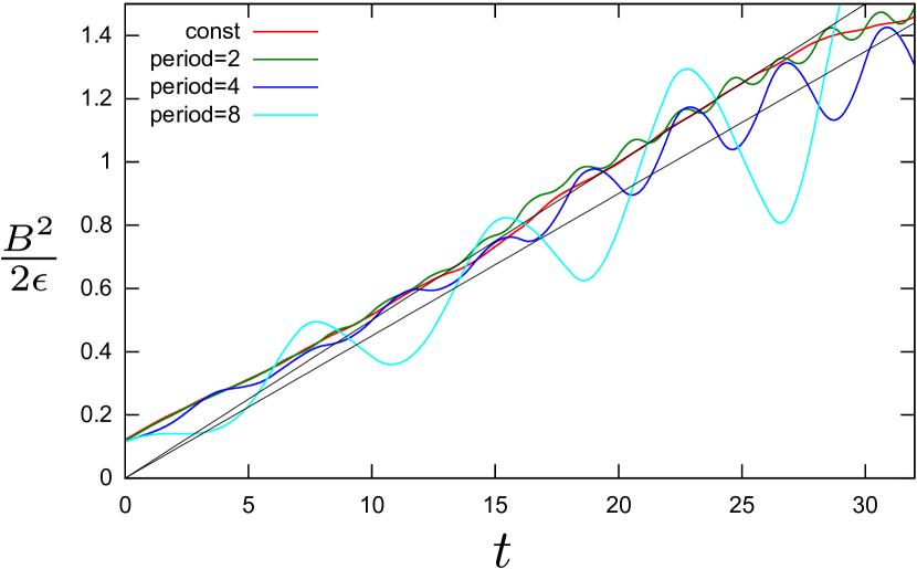
Figure 2.— We plotted the magnetic energy, $B^{2}/2$ (Alfvén units), divided by the energy driving rate, $\epsilon$, resulting in $B^{2}/2\epsilon$ (simulation time units) versus time (simulation time units), similar to results reported in Beresnyak (2012). Several curves correspond to intermittent driving with the period of driving varied from 1 to 8 $\tau_{c}$ and the half of the period the driving was on while the other half off. We also put a simulation with constant driving for comparison. Two thin lines correspond to the conversion efficiencies of nonlinear dynamo $C_{E}$ of 0.045 and 0.05 (dimensionless).

Figure 3.— The relation between magnetic energy and the outer scale in the DNS of nonlinear small scale dynamo. The upper plot correspond to the case with constant driving, reported earlier in Beresnyak (2012), while the lower plot has been produced in otherwise similar simulation with intermittent driving with period of $8\tau_{c}$ (self-correlation timescales). In the case of intermittent driving we used the dissipation rate $\epsilon$ averaged over $2\tau_{c}$ in a manner similar to the analysis of cluster data. We defined outer scale of magnetic field through its peak wavenumber of the spectrum $L_{B}=2\pi/k_{\rm max}$. The best fit corresponds to the coefficient $c_{l}\approx 0.18$ in Eq. (5).

5. Cluster simulations

We use the Matryoshka run to extract the time dependent turbulence properties of the ICM of a massive GC, with total mass at redshift $z=0$ of $1.3\times 10^{15}M_{\odot}$, forming in a concordance $\Lambda$-CDM universe (Komatsu et al., 2009). The simulation was carried out with CHARM, an Adaptive-Mesh-Refinement cosmological code (Miniati & Colella, 2007). We use a concordance $\Lambda$-CDM universe with normalized (in units of the critical value) total mass density, $\Omega_{m}=0.2792$, baryonic mass density, $\Omega_{b}=0.0462$, vacuum energy density, $\Omega_{\Lambda}=1-\Omega_{m}=0.7208$, normalized Hubble constant $h\equiv H_{0}/100$ km s^-1 Mpc^-1 = 0.701, spectral index of primordial perturbation, $n_{s}=0.96$, and rms linear density fluctuation within a sphere with a comoving radius of 8 $\,h^{-1}$ Mpc, $\sigma_{8}=0.817$ (Komatsu et al., 2009). The simulated volume has comoving size of $L_{Box}=240\,h^{-1}$ Mpc on a side. The initial conditions were generated on three refinement levels with grafic++ (made publicly available by D. Potter). For the coarsest level we use 512³ comoving cells, corresponding to a nominal spatial resolution of 468.75$\,h^{-1}$ comoving kpc and 512³ particles of mass $6.7\times 10^{9}\,h^{-1}$ $M_{\odot}$ to represent the collisionless dark matter component. The additional levels allow for refined initial conditions in the volume where the galaxy cluster forms. The refinement ratio for both levels is, $n_{\mathrm{ref}}^{\ell}\equiv\Delta x_{\ell}/\Delta x_{\ell+1}=2$, $\ell=0,1$. Each refined level covers 1/8 of the volume of the next coarser level with a uniform grid of 512³ comoving cells while the dark matter is represented with 512³ particles. At the finest level the spatial resolution is $\Delta x=$ 117.2$\,h^{-1}$ comoving kpc and the particle mass is $10^{8}\,h^{-1}$ M_⊙. As the Lagrangian volume of the galaxy cluster shrinks under self-gravity, three additional uniform grids covering 1/8 of the volume of the next coarser level were employed with 512³, 1024³ and 1024³ comoving cells, respectively, and $n_{\mathrm{ref}}^{\ell}=2,4,2$, for $\ell=2,3,4$, respectively. All of them were in place by redshift 1.4, providing a spatial resolution of 7.3 h^-1 comoving kpc in a region of 7.5 h^-1 Mpc, accommodating the whole virial volume of the GC. The ensuing dynamic range of resolved spatial scales is sufficiently large for the emergence of turbulence. The results of the cluster simulation is described in full detail in (Miniati, 2014, 2015).

6. Analysis of cluster simulations

Using a Hodge-Helmholtz decomposition it was found that between 60 and 90% of the kinetic energy of the cluster turbulence is in the solenoidal component (Miniati, 2015, see also Federrath et al. (2011)). This is the relevant component for the discussed small-scale dynamo mechanism and the key question is whether it resembles homogeneous isotropic turbulence in the inertial range.

In Fig 4, upper panel we checked statistical isotropy of the cluster turbulence. We compared the longitudinal velocity structure function (SF) with the analytical expression that presumes statistical isotropy. Statistical isotropy seems to be satisfied quite well on all scales of interest consistent with results in (Miniati, 2015). A more critical test is provided by the relation between structure functions of different order. For example the dimensionless ratio $\langle(\delta v_{l})^{2}\rangle^{3/2}/\langle(\delta v_{\|l})^{3}\rangle$ is of interest to relate the energy cascade rate with the energy content of the cascade. In the lower panel of Fig 4 we studied the comparison between this ratio in the cluster simulation and in the homogeneous incompressible driven turbulence. For the latter we used data from fully resolved direct numerical simulation of incompressible hydrodynamic driven turbulence in a periodic box, see, e.g. Beresnyak & Lazarian (2009). Both cluster and box simulation exhibited a clear well-pronounced dissipation interval which we used to convert box simulation units into physical scale units of the cluster simulation. Note, however, that no fitting has been involved on the y-axis. Given relatively short inertial range the correspondence between homogeneous isotropic turbulence statistics and cluster statistics is quite remarkable. From the above comparison we conclude that the second order structure function of the cluster simulations in the range of scales 0.14-0.4 Mpc could be reliably used to estimate the turbulent dissipation rate, $\epsilon_{turb}$, associated with the incompressible velocity component and necessary to evaluate dynamo action in the ICM.

Figure 4.— We used structure functions to test statistical isotropy of the given cluster simulations (upper panel). Also we compare the relation between second order total structure function and the third order parallel structure functions in the cluster simulation (solid line) and in a periodic box simulation of statistically stationary driven turbulence (dashed line), after rescaling the dissipation scale to the same number (lower panel). Note that no fitting has been involved in making the both figures. We conclude that the second order structure function in the range 0.14-0.4 Mpc could be used to robustly estimate the turbulent dissipation rate associated with the solenoidal velocity component.

The turbulence dissipation rate is then estimated as follows:

$$\epsilon_{turb}=(c_{1}/c_{2})(5/4)\langle(\delta v_{l})^{2}\rangle^{3/2}/l,$$ (3)

where $c_{2}\approx 27$ is the ratio of the structure functions reported in Fig. 4 and $c_{1}\approx 1.17$ is a factor to correct for dissipation effects, as in our finite Re simulations the Kolmogorov’s -4/5 normalization slightly underestimates the turbulent dissipation rate.

As expected, at a given time $\epsilon_{turb}$ is a rather constant function of $l$ within the inertial range. The observed deviation was used to estimate the error of the measurement of $\epsilon_{turb}$. We plotted the dissipation rate determined in this manner on the top panel of Fig 5. We used the velocity structure function calculated within 1/3 of the virial radius of the simulated cluster for each data-cube. As we see from this figure, the dissipation rate varies non monotonically over roughly an order of magnitude in scale over the lifetime of the cluster. The errorbars defined above indicate the deviation from Kolmogorov’s self-similarity and were rather small, except for the time intervals where the rate was changing rapidly, i.e. the cluster was either relaxing of experiencing a fresh injection of kinetic energy.

Figure 5.— The evolution of the turbulent dissipation rate (upper plot), Alfvén speed (middle) and the outer scale of the magnetic field (bottom) inferred from the cosmological cluster simulation by using self-similar laws for turbulence and dynamo tested and normalized in well-resolved high-$Re$ DNS. In obtaining $v_{A}$, we divided the magnetic energy $E_{B}$ from Eq. 4 to the average density within 1/3 of the virial radius.

We then estimated magnetic energy density as (Beresnyak, 2012)

$$E_{B}=\int_{0}^{t}C_{E}\rho\epsilon_{turb}dt$$ (4)

with $C_{E}=0.05$. We plotted Alfvén velocity on the middle panel of Fig 5. Furthermore, as was shown in Beresnyak (2012), for statistically stationary turbulence the magnetic energy containing scale could be estimated as

$$L_{B}=c_{l}v_{A}^{3}/\epsilon_{turb},$$ (5)

where $c_{l}\approx 0.18$ is a universal coefficient, which could be determined in DNS, see Fig. 3. Our cluster turbulence was rather non-stationary, however, as discussed in Section 4, the estimate Eq. (5) can also be applied to non-stationary driven turbulence as long as the dissipation rate is averaged over a timescale around one dynamical time, see below. This is because hydrodynamic cascade has a memory over around one dynamical time and the changes in the driving rate do not instantaneously affect turbulent rate on small scales (Section 4). So, in using Eq. (5) we used the $\epsilon_{turb}$ averaged over 2 Gyr, which approximately corresponds to two dynamical times.

The middle and bottom panels of Fig 5 show time evolution of the average RMS Alfvén speed, $v_{A}=(2E_{B}/\rho)^{1/2}$ and the magnetic outer scale $L_{B}$. Note that while $v_{A}$ grows monotonically, $L_{B}$ can decrease somewhat during prolonged increase of the turbulent activity, such as during several major mergers.

Our estimates for $z\sim 0$ characteristic values of Alfvénic speed $v_{A}\sim 10^{7}\rm cm/s$ and the outer scales $L_{B}\sim 30-50$ kpc, are consistent with the observed values reported in the literature (McNamara & Nulsen, 2007; Eilek & Owen, 2002; Bonafede et al., 2010; Govoni et al., 2006, 2010). This indicates that the type of nonlinear dynamo described in Beresnyak (2012) is probably operating in clusters, while kinematic models would be challenged to achieve this.

One interesting conclusion from our results on Fig 5 is that the outer scale of the magnetic field grows relatively quickly after the beginning of the simulation. This is different from direct MHD cluster simulations that have mostly kinematic growth with a magnetic spectrum peaked on numerical dissipation scale, e.g., Xu et al. (2012). Note that the scale of the magnetic field plays crucial role in cosmic ray escape times, therefore correctly estimating magnetic outer scale is essential for models of particle acceleration in clusters (see, Brunetti & Lazarian, 2007, 2011; Beresnyak et al., 2013; Miniati, 2015).

7. Discussion

Similar idea based on post-processing of hydrodynamic data was also employed in Ryu et al. (2008), but with substantial differences. The turbulence in these early calculations was not as resolved as in ours, and the growth of magnetic energy and Alfvén scale were not estimated from the turbulent dissipation rate and the precise estimate of $C_{E}$, as we did here.

One of the differences between cluster turbulence and the kind of statistically stationary turbulence studied in Beresnyak (2012) was the strong variations of the cascade rate over timescales of 1-2 dynamical timescales of the cluster. Our estimates of the efficiency in the case of intermittent driving from this work are roughly compatible with $C_{E}=0.05$ and further work with higher Re is expected to clarify whether the differences between constant and intermitted driving are significant. We concluded that the effects of intermittent driving could probably be ignored at the level of precision of the $\epsilon_{turb}$ measurement.

The actual calculation for the evolution of $v_{A}$ and $L_{B}$ was started at time 4.5 Gyr. This artificially assumes that $\epsilon_{turb}$ was zero for all times earlier than $4.5$ Gyr. However, we find that despite this fairly unrealistic assumption, the values of $v_{A}$ and $L_{B}$ quickly converge to the asymptotic values and, as we argued above, this initial state is quickly forgotten. All basic properties of the cluster, such as its mass, size and thermal energy continue to grow along with its magnetic energy and magnetic outer scale. The detailed comparison between thermal, turbulent and magnetic energy components of the cluster has been performed in our companion paper (Miniati & Beresnyak, 2015). There it is found that the fraction of the thermal energy arising from the turbulent dissipation rate changes relatively little over the cosmological time and the turbulent Mach number is also rather stable. Since the magnetic energy is also a fraction of the accumulated turbulent dissipation rate, the plasma $\beta$ in our cluster fluctuates around a constant value $\sim 40$ for the past 10 Gyr (Miniati & Beresnyak, 2015).

Our treatment of cluster turbulence with ILES, as well modeling the evolution of the magnetic energy with the model from Beresnyak (2012) relies on an assumption that the Reynolds numbers in clusters are high. For example, our comparison of the cluster simulation and the DNS leads to an estimate of an effective Kolmogorov (dissipation) scale for the cluster simulation of $\eta\approx 2.7$ kpc, corresponding to an effective $Re$ around 3000. We actually expect clusters to have higher $Re$, as briefly discussed in Section 1, due to the collective microscopic scattering in the high-$\beta$ ICM plasma (Schekochihin & Cowley, 2006; Lazarian & Beresnyak, 2006; Schekochihin et al., 2008; Brunetti & Lazarian, 2011). An important observational test to the problem of the ICM viscosity are the measurements of Faraday rotation in AGN sources located in clusters, which allowed to probe sub-kiloparsec scales due to relatively high resolution of radio maps (Kuchar & Enßlin, 2011; Laing et al., 2008; Govoni et al., 2010). The inferred magnetic spectrum in these measurements is negative and steep, typically around Kolmogorov in the range of scales below 5 kpc and down to the resolution limit. Such a magnetic spectrum is expected from MHD turbulence with small dissipation scales. It would be grossly inconsistent with magnetic spectra obtained in either kinematic dynamo models, due to their positive spectral indexes, or with MHD models using Spitzer viscosity, which would typically give rather shallow spectrum with index around $-1$, see, e.g. Cho et al. (2002). We conclude that even though it is quite obvious that magnetic Prandtl numbers in the ICM are very high, the viscosity is not large enough to affect magnetic spectrum above 1 kpc. Therefore, just from this observational constraint we expect the $Re$ in clusters to be at least $10^{4}$ and probably much higher. Our calculation relied on this fact and the results, grossly consistent with the current observational properties of clusters, provide another support for the picture of a turbulent ICM, as opposed to an earlier view of a viscous and laminar ICM.

References

- Beresnyak (2012) Beresnyak, A. 2012, Phys. Rev. Lett., 108, 035002
- Beresnyak & Lazarian (2006) Beresnyak, A., & Lazarian, A. 2006, ApJ , 640, L175
- Beresnyak & Lazarian (2009) —. 2009, Astrophys. J., 702, 1190
- Beresnyak et al. (2013) Beresnyak, A., Xu, H., Li, H., & Schlickeiser, R. 2013, Astrophys. J., 771, 131
- Bonafede et al. (2010) Bonafede, A., Feretti, L., Murgia, M., Govoni, F., Giovannini, G., Dallacasa, D., Dolag, K., & Taylor, G. B. 2010, A&A , 513, A30
- Brandenburg & Subramanian (2005) Brandenburg, A., & Subramanian, K. 2005, Phys. Rep. , 417, 1
- Brunetti & Lazarian (2007) Brunetti, G., & Lazarian, A. 2007, MNRAS , 378, 245
- Brunetti & Lazarian (2011) Brunetti, G., & Lazarian, A. 2011, Monthly Notices of the Royal Astronomical Society, 410, 127
- Brunetti & Lazarian (2011) Brunetti, G., & Lazarian, A. 2011, MNRAS , 412, 817
- Cho et al. (2002) Cho, J., Lazarian, A., & Vishniac, E. T. 2002, ApJ , 566, L49
- Cho et al. (2009) Cho, J., Vishniac, E. T., Beresnyak, A., Lazarian, A., & Ryu, D. 2009, Astrophys. J., 693, 1449
- Clarke (2004) Clarke, T. E. 2004, Journal of the Korean Astronomical Society, 37, 337
- Clarke et al. (2001) Clarke, T. E., Kronberg, P. P., & Böhringer, H. 2001, The Astrophysical Journal, 547, L111
- Dolag et al. (2002) Dolag, K., Bartelmann, M., & Lesch, H. 2002, Astronomy and Astrophysics, 387, 383
- Dubois & Teyssier (2008) Dubois, Y., & Teyssier, R. 2008, Astronomy and Astrophysics, 482, L13
- Eilek & Owen (2002) Eilek, J. A., & Owen, F. N. 2002, Astrophys. J., 567, 202
- Federrath et al. (2011) Federrath, C., Sur, S., Schleicher, D. R. G., Banerjee, R., & Klessen, R. S. 2011, Astrophys. J., 731, 62
- Ferrari et al. (2008) Ferrari, C., Govoni, F., Schindler, S., Bykov, A. M., & Rephaeli, Y. 2008, Space Science Reviews, 134, 93
- Galeev & Sagdeev (1979) Galeev, A., & Sagdeev, R. 1979, in Reviews of Plasma Physics, Volume 7, Vol. 7, 257
- Govoni et al. (2006) Govoni, F., Murgia, M., Feretti, L., Giovannini, G., Dolag, K., & Taylor, G. B. 2006, A&A , 460, 425
- Govoni et al. (2010) Govoni, F., Dolag, K., Murgia, M., Feretti, L., Schindler, S., et al. 2010, A&A , 522, A105
- Haugen et al. (2004) Haugen, N. E., Brandenburg, A., & Dobler, W. 2004, Phys. Rev. E, 70, 016308
- Kazantsev (1968) Kazantsev, A. P. 1968, Soviet Journal of Experimental and Theoretical Physics, 26, 1031
- Komatsu et al. (2009) Komatsu, E., Dunkley, J., Nolta, M. R., Bennett, C. L., Gold, B., et al. 2009, The Astrophysical Journal Supplement, 180, 330
- Kraichnan & Nagarajan (1967) Kraichnan, R. H., & Nagarajan, S. 1967, Physics of Fluids, 10, 859
- Kuchar & Enßlin (2011) Kuchar, P., & Enßlin, T. A. 2011, Astronomy and Astrophysics, 529, 13
- Kulsrud & Anderson (1992) Kulsrud, R. M., & Anderson, S. W. 1992, Astrophys. J., 396, 606
- Laing et al. (2008) Laing, R. A., Bridle, A. H., Parma, P., & Murgia, M. 2008, Monthly Notices of the Royal Astronomical Society, 391, 521
- Lazarian & Beresnyak (2006) Lazarian, A., & Beresnyak, A. 2006, MNRAS , 373, 1195
- McNamara & Nulsen (2007) McNamara, B. R., & Nulsen, P. E. J. 2007, Phys. Rev. ARA&A, 45, 117
- Miniati (2014) Miniati, F. 2014, The Astrophysical Journal, 782, 21
- Miniati (2015) —. 2015, The Astrophysical Journal, 800, 60
- Miniati & Beresnyak (2015) Miniati, F., & Beresnyak, A. 2015, Nature, in press
- Miniati & Colella (2007) Miniati, F., & Colella, P. 2007, Journal of Computational Physics, 227, 400
- Miniati et al. (2001) Miniati, F., Jones, T. W., Kang, H., & Ryu, D. 2001, The Astrophysical Journal, 562, 233
- Norman & Bryan (1999) Norman, M. L., & Bryan, G. L. 1999, in The radio galaxy Messier 87 : proceedings of a workshop held at Ringberg Castle (Springer Berlin Heidelberg), 106–115
- Ryu et al. (2008) Ryu, D., Kang, H., Cho, J., & Das, S. 2008, Science, 320, 909
- Ryu et al. (2008) Ryu, D., Kang, H., Cho, J., & Das, S. 2008, Science, 320, 909
- Schekochihin & Cowley (2006) Schekochihin, A. A., & Cowley, S. C. 2006, Physics of Plasmas, 13, 056501
- Schekochihin et al. (2008) Schekochihin, A. A., Cowley, S. C., Kulsrud, R. M., Rosin, M. S., & Heinemann, T. 2008, Physical Review Letters, 100, 081301
- Schekochihin et al. (2004) Schekochihin, A. A., Cowley, S. C., Taylor, S. F., Maron, J. L., & McWilliams, J. C. 2004, Astrophys. J., 612, 276
- Schlüter & Biermann (1950) Schlüter, A., & Biermann, I. 1950, Zeitschrift Naturforschung Teil A, 5, 237
- Vazza et al. (2014) Vazza, F., Brüggen, M., Gheller, C., & Wang, P. 2014, Monthly Notices of the Royal Astronomical Society, 445, 3706
- Vazza et al. (2011) Vazza, F., Brunetti, G., Gheller, C., Brunino, R., & Brüggen, M. 2011, Astronomy and Astrophysics, 529, 17
- Xu et al. (2012) Xu, H., Govoni, F., Murgia, M., Li, H., Collins, D. C., et al. 2012, Astrophys. J., 759, 40