Renormalization Group Evolution of Flavour Invariants

Abstract

The fermion spectrum in the Standard Model (SM) exhibits hierarchical structures between the eigenvalues of the Yukawa matrices which determine the fermion masses, as well as certain hierarchical patterns in the mixing matrix that describes weak transitions between different fermion generations. A basis-independent description of the SM flavour structure can be given in terms of a complete set of flavour invariants. In this paper, we construct a convenient set of such invariants, and discuss the general form of the renormalization-group equations. We also discuss the simplifications that arise from exploiting hierarchies in Yukwawa couplings and mixings which are present in the SM or its minimal-flavour violating extensions.

1 Introduction

In the Standard Model (SM) of particle physics, the Yukawa couplings of quarks and charged leptons to the Higgs field are the only sources of flavour structure. The singular values of the Yukawa matrices, together with the vacuum expectation value (VEV) of the Higgs field determine the fermion masses, and the relative orientation between the up- and down-quark Yukawa matrices results in the Cabibbo-Kobayashi-Maskawa (CKM) matrix, responsible for charged flavour transitions in weak interactions. In the quantum-field theoretical formulation of the SM, the Yukawa matrices enter as coupling parameters in the Lagrange density. In the following, we will focus on the quark sector, where one has

$$-{\cal L}_{\rm Yukawa} =Y_{U}^{ij}\,\bar{Q}_{L}^{i}\widetilde{H}\,U_{R}^{j}+Y_{D}^{ij}\,\bar{Q}_{L}^{i}H\,D_{R}^{j}+\mbox{h.c.}$$ (1)

Here and in the following $Y_{U}$ and $Y_{D}$ denote the Yukawa matrices for up- and down-type quarks, $Q_{L},U_{R},D_{R}$ are the left-handed quark doublet and right-handed singlets, respectively, and $H,\widetilde{H}$ is the Higgs field and its $SU(2)$ conjugate. The indices $i,j=1\ldots n_{g}$ denote the quark generations/families ($n_{g}=3$ in the SM).

As all other couplings in the SM, after renormalization of ultraviolet divergencies, the Yukawa matrices in (1) are to be interpreted as effective parameters with the scale-dependence controlled by renormalization-group (RG) equations Machacek:1983fi ; Grzadkowski:1987tf ; Arason:1991ic ; Barger:1992pk . The structure of the RG equations and their solutions have been extensively studied in the past. In Balzereit:1998id , the resulting one-loop RG evolution of the CKM matrix elements (in a given parametrization) has been studied, and approximate analytic solutions have been derived on the basis of the observed hierachies in quark masses and mixing angles in the SM. Generalizations to particular new physics (NP) frameworks have also been derived, notably for 2-Higgs-doublet models or supersymmetric extensions of the SM, see, for instance, Das:2000uk ; Crivellin:2008mq . Recently, the effect of possible NP contributions has been studied in a model-independent way, by considering the RG effects from dimension-six operators in an effective field theory (SM-EFT) approach Jenkins:2013wua . Finally, Bednyakov et al. Bednyakov:2014pia have recently computed the three-loop RG coefficients for the SM Yukawa matrices.

The RG equations are usually formulated in matrix form, i.e. the scale-variation of the Yukawa matrices is given by a matrix polynomial of $Y_{U}$ and $Y_{D}$. Since the gauge sector of the SM is invariant under unitary field redefinitions for the individual quark multiplets, the RG equations have to transform covariantly under such changes of flavour basis (see below). This also implies a certain degree of redundancy in the RG equations, because from the 18 complex matrix entries in $Y_{U}$ and $Y_{D}$ only 10 physical parameters are observables.

In this paper, we will therefore reformulate the RG equations in terms of flavour invariants, i.e. objects constructed from $Y_{U}$ and $Y_{D}$ which are independent of the choice of flavour basis. As has been shown in Jenkins:2009dy from the basic algebraic principle of Hilbert series, one can define eleven polynomially independent flavour invariants for three quark generations. These fix the six quark masses, the three mixing angles and the sine and cosine of the CP-violating phase in the CKM matrix. As a corollary, using Cayley-Hamilton identities for matrix products (cf. Colangelo:2008qp ), this also implies that any flavour-covariant product of Yukawa matrices that appears on the right-hand side of the RG equations for $Y_{U}$ or $Y_{D}$ can be reduced to a finite basis of flavour matrices with coefficients given as polynomials of flavour invariants. It is then a straightforward, though tedious, task to derive the RG equations for the set of flavour invariants.

Although the RG equations for the flavour invariants contain the same information as the original flavour-covariant equations, the formulation in terms of flavour invariants, under certain circumstances, may be considered advantageous. For instance, the form of the RG equations is universal, not only for the SM, but also for all extensions that obey the principle of minimal flavour violation (MFV) in the technical sense of D'Ambrosio:2002ex . Furthermore, the hierachical pattern of masses and mixing directly translates into a well-defined power counting for (suitably chosen) flavour invariants, which can be exploited to simplify the RG equations. An attractive physical picture arises if one assumes these hierarchies to be associated to some dynamical NP mechanism that can be traced back to an effective potential which determines the flavour structures at low energies. Within the MFV framework, the potential itself will have to be formulated in terms of flavour invariants, and the minimization of the potential should generate VEVs for the flavour invariants that reflect the particular pattern of (sequential) flavour-symmetry breaking in the SM (see Feldmann:2009dc ). Recent studies along these lines can be found, for instance, in Alonso:2011yg ; Nardi:2011st ; Espinosa:2012uu ; Fong:2013dnk . Finally, our approach could be extended and generalized to cases where there are additional flavour structures in some tensor representation of the SM flavour symmetry group. For example, these could show up as coupling constants in front of higher-dimensional operators in SM-EFT Buchmuller:1985jz ; Grzadkowski:2010es , or as new spurion fields in the MFV framework Feldmann:2006jk ; Isidori:2012ts .

The remaining paper is organized as follows: In the next section, we will first discuss a toy scenario with only two generations (2G) of SM quarks. The simplifications in the 2G case (no CP violation, closure of $SU(2)$ matrices under multiplication, small number of polynomially independent invariants) allow us to introduce our approach in a very transparent way, perform all calculations analytically and illustrate the RG equations for the flavour invariants in a graphical way. To this end, we will first give convenient definitions for flavour invariants and basic flavour matrices. In terms of these, the general form of the RG equations for flavour invariants will be derived. We also present analytical and numerical solutions for the RG equations that can be obtained from exploiting SM-like flavour hierarchies in the one-loop approximation. In Section 3 we generalize our framework to the realistic case of three quark generations (3G). To keep the discussion transparent, we restrict ourselves to the one-loop approximation from the very beginning. Again, we derive the general form of the (one-loop) RG equations for the eleven flavour invariants, and discuss their approximate solutions in the SM. We close the paper with a short summary and outlook in Section 4. Some technical details about the use of Cayley-Hamilton identities, the explicit form of the 3G flavour invariants, and the general form of the two-loop RG equations in the 3G case can be found in the appendices.

2 Two Quark Generations

As mentioned above, in this section, we restrict ourselves to two generations of left-handed quark doublets and right-handed up- and down-quark singlets in the SM. The gauge-kinetic terms of the SM Lagrangian are flavour-blind, and therefore independent unitary rotations of the quark multiplets define a flavour symmetry,

$${\cal G}_{\rm quark} =U(2)^{3}/U(1)_{B}\ \sim\ SU(2)_{Q_{L}}\times U(2)_{U_{R}}\times U(2)_{D_{R}}\,,$$ (2)

which is only broken by the Yukawa couplings in (1). Here we factored out a $U(1)_{B}$ symmetry for baryon number conservation, which is unaffected by the SM Yukawa interactions Feldmann:2009dc . (More precisely, we find it convenient to factor out a $U(1)_{Q_{L}}$ transformation acting on the left-handed doublets only). In a particular flavour basis, the Yukawa matrices for up- and down-type quarks read

$$Y_{U}=\left(\begin{array}[]{cc}y_{u}&0\\ 0&y_{c}\end{array}\right)\,, \qquad Y_{D}=V_{\rm Cabbibo}\left(\begin{array}[]{cc}y_{d}&0\\ 0&y_{s}\end{array}\right)=\left(\begin{array}[]{cc}\cos\theta&\sin\theta\\ -\sin\theta&\cos\theta\end{array}\right)\left(\begin{array}[]{cc}y_{d}&0\\ 0&y_{s}\end{array}\right)\,.$$ (11)

Under a change of flavour basis, the Yukawa matrices transform as

$$Y_{U} \to V_{Q_{L}}\,Y_{U}\,V_{U_{R}}^{\dagger}\,,\qquad Y_{D}\to V_{Q_{L}}\,Y_{D}\,V_{D_{R}}^{\dagger}\,,$$ (12)

where $V_{Q_{L}}\in SU(2)_{Q_{L}}$ etc.

2.1 Flavour Invariants

In the 2G case, one can construct five flavour invariants that are polynomially independent (see e.g. Jenkins:2009dy and references therein for the mathematical background). In the following, to set the stage for the 3G case to be discussed in Sec. 3, we will discuss the construction and properties of these flavour invariants step by step.

From the Yukawa matrices $Y_{U}$ and $Y_{D}$, one can construct flavour invariants in terms of traces or determinants of matrix products constructed from the non-negative hermitian matrices

$$U=Y_{U}Y_{U}^{\dagger}\,,\qquad D=Y_{D}Y_{D}^{\dagger}\,.$$ (13)

These transform as $V_{Q_{L}}U\,V_{Q_{L}}^{\dagger}$ and $V_{Q_{L}}D\,V_{Q_{L}}^{\dagger}$ under basis tranformations for the left-handed quark doublets. A convenient choice for non-negative invariants is

$$I_{1}\equiv\text{tr}[U]=y_{u}^{2}+y_{c}^{2}\geq 0\,, I_{2}\equiv\text{tr}[D]=y_{d}^{2}+y_{s}^{2}\geq 0\,,$$ (14)

$$\widehat{I}_{3}\equiv\det[U]=y_{u}^{2}y_{c}^{2}\geq 0 \widehat{I}_{4}\equiv\det[D]=y_{d}^{2}y_{s}^{2}\geq 0\,,$$ (15)

and

$$\widehat{I}_{5}\equiv\text{tr}[UD]=(y_{c}^{2}y_{s}^{2}+y_{d}^{2}y_{u}^{2})\cos^{2}\theta+(y_{c}^{2}y_{d}^{2}+y_{s}^{2}y_{u}^{2})\sin^{2}\theta\geq 0\,.$$ (16)

Apart from discrete ambiguties related to renaming the original quark fields in the flavour eigenbasis, they determine the four eigenvalues for the Yukawa couplings and the Cabibbo mixing angle. Invariants built from traces of higher powers of $U$ and $D$ are related to the above via Cayley-Hamilton identities (see appendix A and e.g. the discussion in Colangelo:2008qp ). Still, for the following discussion, we further define the polynomially dependent invariants

$$I_{3}\equiv\frac{I_{1}^{2}}{2}-2\widehat{I}_{3}=\frac{1}{2}(y_{c}^{2}-y_{u}^{2})^{2}\,,\qquad I_{4}\equiv\frac{I_{2}^{2}}{2}-2\widehat{I}_{4}=\frac{1}{2}(y_{s}^{2}-y_{d}^{2})^{2}\,,$$ (17)

and

$$I_{5} \equiv\widehat{I}_{5}-\frac{I_{1}I_{2}}{2}=\frac{1}{2}(y_{c}^{2}-y_{u}^{2})(y_{s}^{2}-y_{d}^{2})\cos(2\theta)\,,$$ (18)

$$\widetilde{I}_{5} \equiv I_{3}I_{4}-I_{5}^{2}=\frac{1}{4}(y_{c}^{2}-y_{u}^{2})^{2}(y_{s}^{2}-y_{d}^{2})^{2}\sin^{2}(2\theta)\,.$$ (19)

Triplet Matrices and Triplet Invariants:

It is further convenient to divide the matrices $U$ and $D$ into singlet and triplet components with respect to the flavour group factor $SU(2)_{Q_{L}}$,

$$U =\frac{1}{2}\,\text{tr}[U]\,\mathds{1}+U_{3}\,,\qquad D=\frac{1}{2}\,\text{tr}[D]\,\mathds{1}+D_{3}\,,$$ (20)

A third independent triplet matrix can be defined as

$$A_{3} =\frac{i}{2}\left[U_{3},D_{3}\right]\,.$$ (21)

Polynomial Basis:

For generic Yukawa entries, any $2\times 2$ matrix $M$ that transforms as $V_{Q_{L}}\,M\,V_{Q_{L}}^{\dagger}$ under $SU(2)_{Q_{L}}$ can be written as a finite polynomial of matrices from the set $\{{\mathds{1}},U_{3},D_{3},A_{3}\}$. For those matrices, the following multiplication tables for symmetric and anti-symmetric products of matrices holds.

$\{\ ,\ \}$	$U_{3}$	$D_{3}$	$A_{3}$
$U_{3}$	$I_{3}\,\mathds{1}$	$I_{5}\,\mathds{1}$	$0$
$D_{3}$	$I_{5}\,\mathds{1}$	$I_{4}\,\mathds{1}$	$0$
$A_{3}$	$0$	$0$	$\frac{1}{2}\widetilde{I}_{5}\,\mathds{1}$

$i\,[\ ,\ ]$	$U_{3}$	$D_{3}$	$A_{3}$
$U_{3}$	$0$	$\phantom{-}2\bar{A}_{3}$	$-2\bar{D}_{3}$
$D_{3}$	$-2\bar{A}_{3}$	$0$	$\phantom{-}2\bar{U}_{3}$
$A_{3}$	$\phantom{-}2\bar{D}_{3}$	$-2\bar{U}_{3}$	$0$

This explicitly shows that the set $\{{\mathds{1}},U_{3},D_{3},A_{3}\}$ closes under matrix multiplication with prefactors that are polynomials of the flavour invariants . Here we defined the dual matrices

$$\bar{U}_{3}\equiv\frac{i}{2}\left[D_{3},A_{3}\right] =\frac{I_{4}}{2}\,U_{3}-\frac{I_{5}}{2}\,D_{3}\,,\qquad\bar{D}_{3}\equiv\frac{i}{2}\left[A_{3},U_{3}\right]=\frac{I_{3}}{2}\,D_{3}-\frac{I_{5}}{2}\,U_{3}\,,$$ (22)

and

$$\bar{A}_{3} \equiv\frac{i}{2}\left[U_{3},D_{3}\right]=A_{3}\,,$$ (23)

which can be obtained from the inverse of the metric

$$G_{XY}={\rm tr}[X_{3}Y_{3}]=\left(\begin{array}[]{ccc}I_{3}&I_{5}&0\\ I_{5}&I_{4}&0\\ 0&0&\frac{\widetilde{I}_{5}}{2}\end{array}\right)\qquad\mbox{($X,Y=U,D,A$),}$$ (27)

as

$$\left(\begin{array}[]{c}\bar{U}_{3}\\ \bar{D}_{3}\\ \bar{A}_{3}\end{array}\right) =\frac{\widetilde{I}_{5}}{2}\,G^{-1}\,\left(\begin{array}[]{c}U_{3}\\ D_{3}\\ A_{3}\end{array}\right)\,.$$ (34)

From this we can read off the orthogonality relations between triplet matrices and their dual,

$$\text{tr}\left[X_{3}\bar{Y}_{3}\right]=\frac{\widetilde{I}_{5}}{2}\,\delta_{XY}\qquad\mbox{($X,Y=U,D,A$).}$$ (35)

This can be used, for instance, to decompose a generic $SU(2)_{Q_{L}}$ triplet matrix as

$$M_{3} =\sum_{X=U,D,A}\frac{2\,\text{tr}[\bar{X}_{3}M_{3}]}{\widetilde{I}_{5}}\,X_{3}\,.$$ (36)

Similarly, a matrix $M_{U}$ that transforms as a bi-doublet under $SU(2)_{Q_{L}}\times SU(2)_{U_{R}}$ can be decomposed as

$$M_{U} =\frac{\text{tr}[M_{U}Y_{U}^{-1}]}{2}\,\mathds{1}+\sum_{X=U,D,A}\frac{2\,\text{tr}[\bar{X}_{3}M_{U}Y_{U}^{-1}]}{\widetilde{I}_{5}}\,X_{3}\,,$$ (37)

and analogously for $U_{R}\leftrightarrow D_{R}$. Higher tensor representations of the flavour symmetry group and their expansion can be constructed from $M_{3,U,D}$. Notice that for generic matrices $M_{3,U,D}$, the coefficients in these expansions are enhanced by $(\widetilde{I}_{5})^{-1}$ and $Y_{U,D}^{-1}$, respectively. In contrast, the MFV hypothesis assumes these coefficients to be of order 1 or smaller (see again Colangelo:2008qp ).

2.2 Renormalization-Group Equations

2.2.1 General Form

The Yukawa matrices are subject to renormalization-group (RG) evolution. The generic form for the RG-running of the Yukawa matrices $Y_{U,D}$ can be written in manifestly flavour-symmetric form (see e.g. Grzadkowski:1987tf ). Using the generic decomposition into basis matrices as discussed above, we thus write

$$\frac{dY_{U}(\mu)}{d\ln\mu} =\left(a_{0}(I_{i},\mu)\,\mathds{1}+a_{1}(I_{i},\mu)\,U_{3}+a_{2}(I_{i},\mu)\,D_{3}+i\,a_{3}(I_{i},\mu)\,A_{3}\right)Y_{U}(\mu)\,,$$ (38)

$$\frac{dY_{D}(\mu)}{d\ln\mu} =\left(b_{0}(I_{i},\mu)\,\mathds{1}+b_{1}(I_{i},\mu)\,D_{3}+b_{2}(I_{i},\mu)\,U_{3}-i\,b_{3}(I_{i},\mu)\,A_{3}\right)Y_{D}(\mu)\,.$$ (39)

Each of the coefficients $a_{i},b_{i}$ depends on flavour invariants which arise from loop diagrams including additional Higgs-Yukawa couplings. (At one-loop accuracy, only terms at most quadratic in the Yukawa couplings can appear within the round brackets etc.) In the SM (or, in general, in constrained MFV models without additional sources of CP violation), the coefficients will be real polynomials of the flavour invariants. This immediately translates into RG equations for the matrices $U$ and $D$, an from this we obtain

$$\frac{dI_{1}}{d\ln\mu} =\text{tr}\left[\frac{dU}{d\ln\mu}\right]=2\left(a_{0}\,I_{1}+a_{1}\,I_{3}+a_{2}\,I_{5}\right)\,,$$ (40)

$$\frac{dI_{2}}{d\ln\mu} =\text{tr}\left[\frac{dD}{d\ln\mu}\right]=2\left(b_{0}\,I_{2}+b_{1}\,I_{4}+b_{2}\,I_{5}\right)\,.$$ (41)

In a similar way, one obtains the RG equations for the remaining invariants in a straightforward manner. The RG equations for the invariants $\widehat{I}_{3}$, $\widehat{I}_{4}$ take a particularly simple form

$$\frac{d\widehat{I}_{3}}{d\ln\mu} =4a_{0}\,\widehat{I}_{3}\,,\qquad\frac{d\widehat{I}_{4}}{d\ln\mu}=4b_{0}\,\widehat{I}_{4}\,.$$ (42)

For the invariant $I_{5}$, we obtain

$$\frac{dI_{5}}{d\ln\mu} =\left(2a_{0}+2b_{0}+a_{1}I_{1}+b_{1}I_{2}\right)I_{5}+a_{2}I_{1}I_{4}+b_{2}I_{2}I_{3}+(a_{3}+b_{3})\,\widetilde{I}_{5}\,,$$ (43)

and for the invariant $\widetilde{I}_{5}$, we get

$$\frac{d\widetilde{I}_{5}}{d\ln\mu} =\left(4a_{0}+4b_{0}+2a_{1}I_{1}+2b_{1}I_{2}-2(a_{3}+b_{3})\,I_{5}\right)\widetilde{I}_{5}\,,$$ (44)

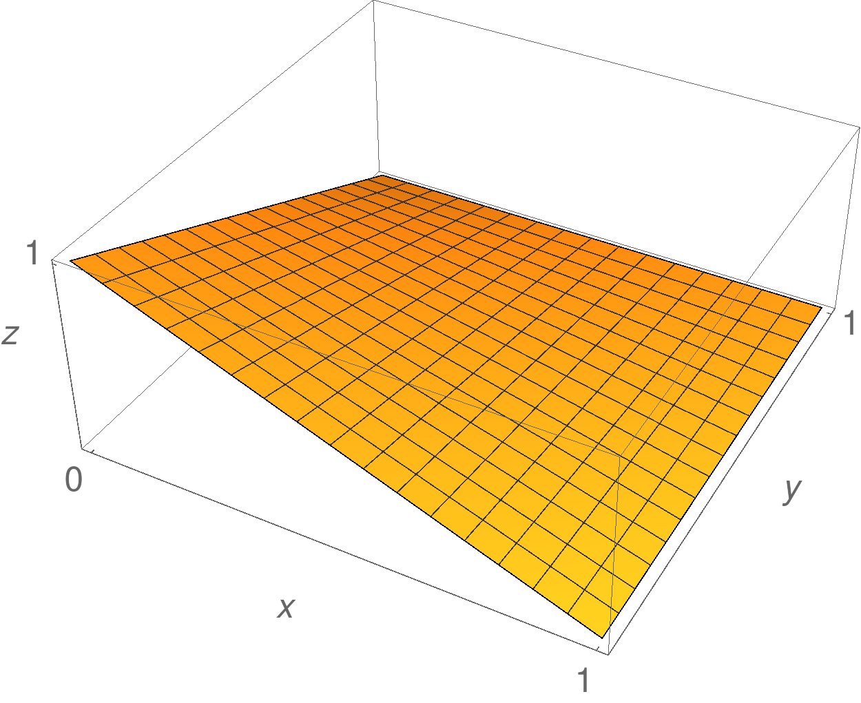
Figure 1: Illustration of the “phase space” (the region below the shaded area) for the normalized invariants $x,y,z$ defined in the text.

Discussion:

From (42) and (44) we observe that some limiting cases in the phase space of flavour invariants are stable under RG evolution:

• The case $\widehat{I}_{3}=0$:
  In terms of physical parameters, this corresponds to one vanishing eigenvalue in the up-quark sector, $y_{u}=0$, and otherwise generic values for $y_{d,s,c}$ and $\theta$.

• The case $\widehat{I}_{4}=0$:
  This corresponds to one vanishing eigenvalue in the down-quark sector, $y_{d}=0$, and otherwise generic values for $y_{u,s,c}$ and $\theta$.

• The case $\widetilde{I}_{5}=0$;
  This corresponds to $\sin 2\theta=0$, i.e. no mixing and otherwise generic $Y_{U}$ and $Y_{D}$; or degenerate eigenvalues in the up-quark sector ($y_{u}=y_{c}$) or in the down-quark sector ($y_{d}=y_{s}$), respectively.

For illustration, we thus define normalized invariants (for $I_{1,2}\neq 0$),

$$x=1-\bar{x}\equiv\frac{4\widehat{I}_{3}}{I_{1}^{2}}\,,\qquad y=1-\bar{y}\equiv\frac{4\widehat{I}_{4}}{I_{2}^{2}}\,,\qquad z=1-\bar{z}\equiv\frac{4\widetilde{I}_{5}}{I_{1}^{2}I_{2}^{2}}\,,$$ (45)

which take values in the unit interval $[0,1]$, with the additional constraints

$$z\leq\bar{x}\,\bar{y}\,.$$ (46)

This is illustrated in Fig. 1. As a consequence of the above observations, there will be now RG flow from the “phase-space” edges, defined by $x=0$, $y=0$, or $z=0$, into the bulk. This can be understood as a consequence of a residual flavour symmetry. In contrast, the case $z=\bar{x}\bar{y}$ is not protected by symmetry. A more detailed discussion of the residual flavour symmetries associated with this situation will be given in Feldmann:2015unp (see also Alonso:2013dba ).

2.2.2 Exploiting Flavour Hierarchies

The RG equations simplify when one exploits flavour hierarchies in the Yukawa matrices. For instance, in a SM-like scenario, we can consider the limit where all but one Yukawa coupling, say $y_{c}$ in the 2G toy case, are small. In this case, the basis of triplet matrices in (39) can be reduced to $U_{3}$, and consequently only the coefficients $a_{0},b_{0},a_{1},b_{2}$ are relevant to first approximation. The RG equations for the invariants in this approximation read (also using $I_{3}\simeq I_{1}^{2}/2$)

$$\frac{dI_{1}}{d\ln\mu} \simeq\left(2a_{0}+a_{1}I_{1}\right)I_{1}\,,\qquad\frac{d\widehat{I}_{3}}{d\ln\mu}=4a_{0}\widehat{I}_{3}\,,$$ (47)

$$\frac{dI_{2}}{d\ln\mu} \simeq 2b_{0}I_{2}+2b_{2}I_{5}\,,\qquad\frac{d\widehat{I}_{4}}{d\ln\mu}=4b_{0}\widehat{I}_{4}\,,$$ (48)

$$\frac{d\widetilde{I}_{5}}{d\ln\mu} \simeq\left(4a_{0}+4b_{0}+2a_{1}I_{1}\right)\widetilde{I}_{5}\,.$$ (49)

Solving for the four coefficients, leaves one general relation between the five invariants and their derivatives which can be written as

$$\frac{d\widetilde{I}_{5}}{\widetilde{I}_{5}} \simeq 2\,\frac{dI_{1}}{I_{1}}+\frac{d\widehat{I}_{4}}{\widehat{I}_{4}}\qquad\mbox{(for $y_{c}\gg y_{u,d,s}$).}$$ (50)

This implies

$$\frac{\widetilde{I}_{5}(\mu)}{\widetilde{I}_{5}(\mu_{0})} \simeq\frac{I_{1}^{2}(\mu)\,\widehat{I}_{4}(\mu)}{I_{1}^{2}(\mu_{0})\,\widehat{I}_{4}(\mu_{0})}\quad\Leftrightarrow\quad\frac{y}{z}\simeq\text{const.}\,,$$ (51)

or, in terms of Yukawa eigenvalues and the Cabibbo angle,

$$\left(y_{s}/y_{d}-y_{d}/y_{s}\right)^{2}\sin^{2}(2\theta)\simeq\mbox{const.}\qquad\mbox{(for $y_{c}\gg y_{u,d,s}$).}$$ (52)

Putting in experimental values for the quark-mass ratio and the Cabibbo angle, the constant on the r.h.s. ranges between 60 and 90.

2.2.3 One-loop Solutions in the SM

$a_{0}$	$b_{0}$	$a_{1}=b_{1}$	$a_{2}=b_{2}$
$\frac{3}{8\pi^{2}}\left(I_{1}+I_{2}+\frac{I_{1}-I_{2}}{2n_{g}}\right)-\frac{2\alpha_{s}}{\pi}$	$\frac{3}{8\pi^{2}}\left(I_{1}+I_{2}+\frac{I_{2}-I_{1}}{2n_{g}}\right)-\frac{2\alpha_{s}}{\pi}$	$\frac{3}{16\pi^{2}}$	$-\frac{3}{16\pi^{2}}$

Table 1: Non-vanishing RG coefficients in the SM as defined in the text, following from Balzereit:1998id . Here $n_{g}$ denotes the number of generations, and electroweak contributions have been neglected for simplicity.

To illustrate the numerical effect of the RG equations, we consider the one-loop RG coefficients in the SM. The system of RG equations further simplifies if we neglect electroweak corrections, leading to the values summarized in Table 1. For the starting values of the invariants in the 2G case, we consider a toy model where we neglect the first generation in the SM, such that the large Yukawa couplings from the third generation lead to non-trivial effects on the r.h.s. of the RG equations. Exploiting again the hierarchies in the SM Yukawa entries, we then find

$$\frac{dI_{1}}{d\ln\mu} \simeq\frac{9}{8\pi^{2}}\,I_{1}^{2}-\frac{4\alpha_{s}}{\pi}\,I_{1}\,.$$ (53)

Using the one-loop expression for the QCD $\beta$-function,

$$\frac{d\alpha_{s}}{d\ln\mu} \simeq-\frac{\beta_{0}}{2\pi}\,\alpha_{s}^{2}\,,$$ (54)

one obtains the explicit solution

$$I_{1}(\mu) \simeq\eta^{8/\beta_{0}}\,I_{1}(\mu_{0})\,G(\mu,\mu_{0})\,,\qquad\eta=\frac{\alpha_{s}(\mu)}{\alpha_{s}(\mu_{0})}$$ (55)

where we defined the RG-evolution function

$$G(\mu,\mu_{0}) :=\exp\left[\frac{9}{8\pi^{2}}\,\int_{\mu_{0}}^{\mu}\frac{d\mu}{\mu}\,I_{1}(\mu)\right]\simeq\left(1+I_{1}(\mu_{0})\,\frac{9}{4\pi}\,\frac{\eta-\eta^{8/\beta_{0}}}{(\beta_{0}-8)\,\alpha_{s}(\mu)}\right)^{-1}\,.$$ (56)

This coincides with Balzereit:1998id , where the approximate RG flow of the top Yukawa coupling has been derived (with $I_{1}(\mu)\simeq(y_{t}(\mu))^{2}$ and $\beta^{(1)}$ in Balzereit:1998id is defined as $\beta^{(0)}/4$ in our convention.) For the remaining invariants, using $y_{c}\gg y_{s}\gg y_{u,d}$ and $|\sin 2\theta|\ll 1$, we have

$$\frac{dI_{2}}{d\ln\mu} \simeq\frac{3}{8\pi^{2}}\,I_{1}I_{2}-\frac{4\alpha_{s}}{\pi}\,I_{2}\qquad\Leftrightarrow\qquad\frac{d(I_{2}/I_{1})}{d\ln\mu}\simeq-\frac{3}{4\pi^{2}}\,I_{1}\left(\frac{I_{2}}{I_{1}}\right)\,,$$ (57)

and

$$\frac{d\widehat{I}_{3}}{d\ln\mu} \simeq\frac{15}{8\pi^{2}}\,I_{1}\widehat{I}_{3}-\frac{8\alpha_{s}}{\pi}\,\widehat{I}_{3} \Leftrightarrow\quad\frac{dx}{d\ln\mu} \simeq-\frac{3}{8\pi^{2}}\,I_{1}\,x\,,$$ (58)

$$\frac{d\widehat{I}_{4}}{d\ln\mu} \simeq\frac{9}{8\pi^{2}}\,I_{1}\widehat{I}_{4}-\frac{8\alpha_{s}}{\pi}\,\widehat{I}_{4} \Leftrightarrow\quad\frac{dy}{d\ln\mu} \simeq\phantom{-}\frac{3}{8\pi^{2}}\,I_{1}\,y\,,$$ (59)

$$\frac{d\widetilde{I}_{5}}{d\ln\mu} \simeq\frac{27}{8\pi^{2}}\,I_{1}\widetilde{I}_{5}-\frac{16\alpha_{s}}{\pi}\,\widetilde{I}_{5} \Leftrightarrow\quad\frac{dz}{d\ln\mu} \simeq\phantom{-}\frac{3}{8\pi^{2}}\,I_{1}\,z\,.$$ (60)

We see that once the RG-solution for $I_{1}(\mu)$ has been constructed, the RG equations for the remaining invariants can be easily solved by separation of variables. Using the RG function $G(\mu,\mu_{0})$ defined in (56), we have

$$I_{2}(\mu) \simeq\eta^{8/\beta_{0}}I_{2}(\mu_{0})\left[G(\mu,\mu_{0})\right]^{1/3}\,,$$ (61)

and

$$x(\mu) \simeq\left[G(\mu,\mu_{0})\right]^{-1/3}x(\mu_{0})\,,\quad y(\mu)\simeq\left[G(\mu,\mu_{0})\right]^{1/3}y(\mu_{0})\,,\quad z(\mu)\simeq\left[G(\mu,\mu_{0})\right]^{1/3}z(\mu_{0})\,.$$ (62)

2.2.4 Numerical Illustration

In Fig. 2 we provide illustrations for the one-loop RG flow of the combinations of flavour invariants $x,y,z$ in the SM, and compare the exact numerical solutions with the approximation in (62). We observe that — for the chosen numerical starting values — even for values as large as $t=\ln\mu/\mu_{0}=15$, the differences between the exact and approximate solutions are always below 5%.

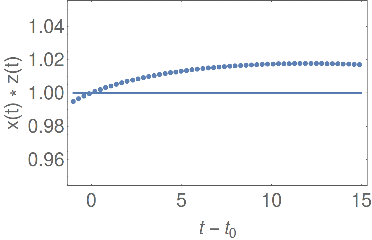
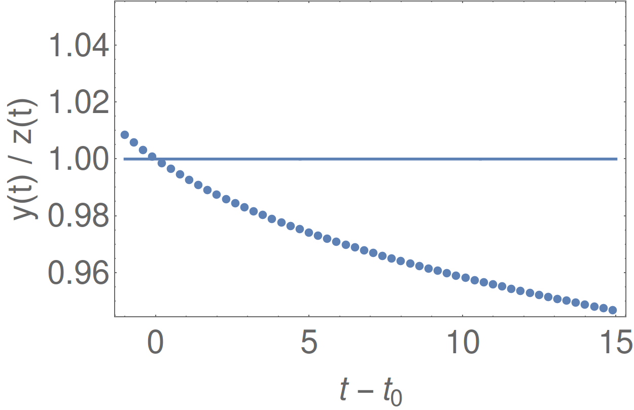
Figure 2: Comparison of numerical [dots] and approximate analytical (62) [solid line] solution for combinations of flavour invariants, $x(t)z(t)$ and $y(t)/z(t)$, normalized to the values at $t=\ln\mu/\mu_{0}\to t_{0}=0$. The following starting values have been used: $I_{1}(t_{0})=1.0$, $I_{2}(t_{0})=0.1$, $x(t_{0})=0.005$, $y(t_{0})=0.048$, $z(t_{0})=0.105$.

In Fig. 3 we illustrate the RG flow for the boundaries of the “phase-space” of flavour invariants, defined by $z\equiv 0$, $y\equiv 0$, $x\equiv 0$, respectively, see the discussion in Section 2.2.1. Again, we have chosen a hierarchical scenario with $I_{2}(\mu_{0})\ll I_{1}(\mu_{0})$. We observe that

• The relation $y(t)/z(t)\simeq\text{const.}$ holds on the whole plane $x=0$, which is in line with our derivation of (51) which only required $I_{1}\gg I_{2}$.

• In contrast, $x(t)y(t)\simeq\text{const.}$ only holds in the vicinity of $x\sim y\sim 0$ (where $y_{u}\ll y_{c}$ and $y_{d}\ll y_{s}$) and for $\theta$ near zero (which requires the solution with $I_{5}(\mu_{0})=-\sqrt{I_{3}I_{4}-\widetilde{I}_{5}}(\mu_{0})I_{5}$ shown on the left-hand side).

• The same is true for $x(t)z(t)\simeq\text{const.}$.

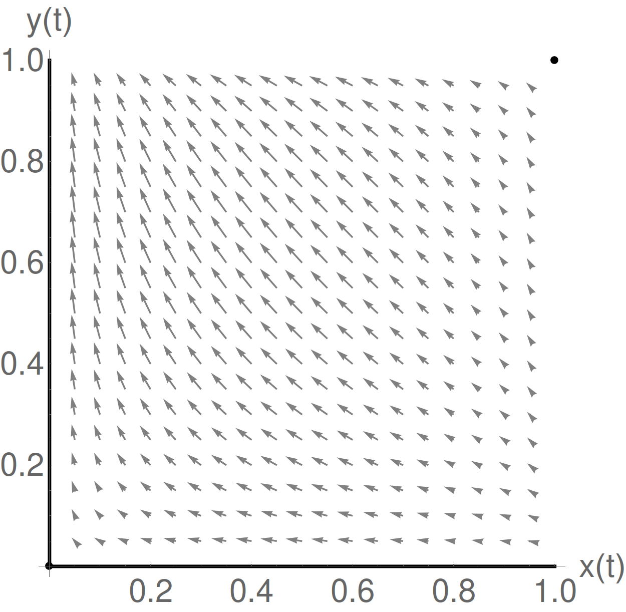
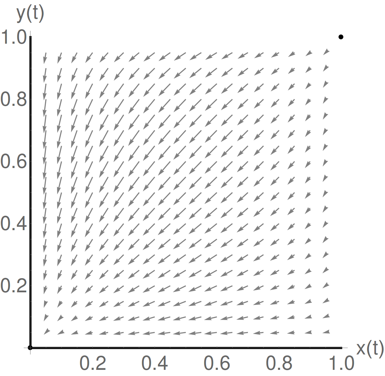
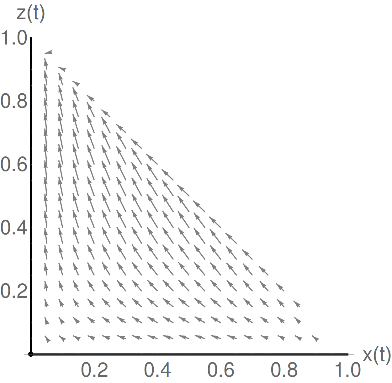
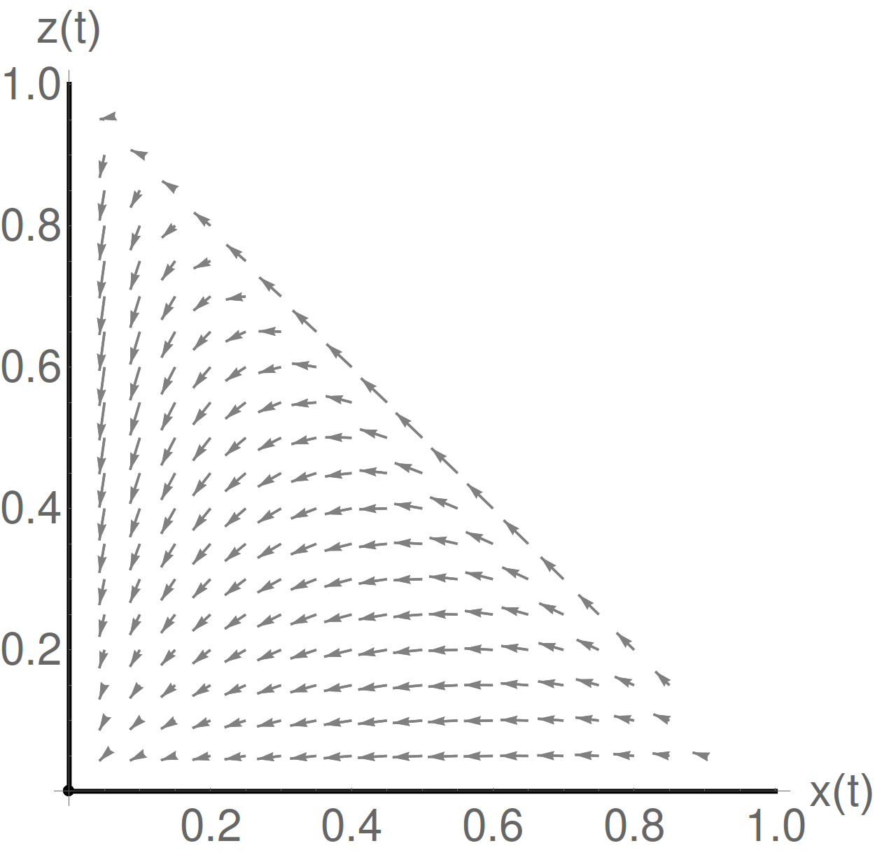
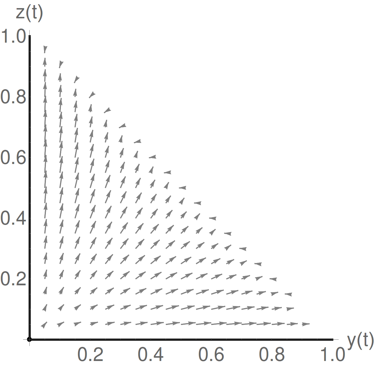
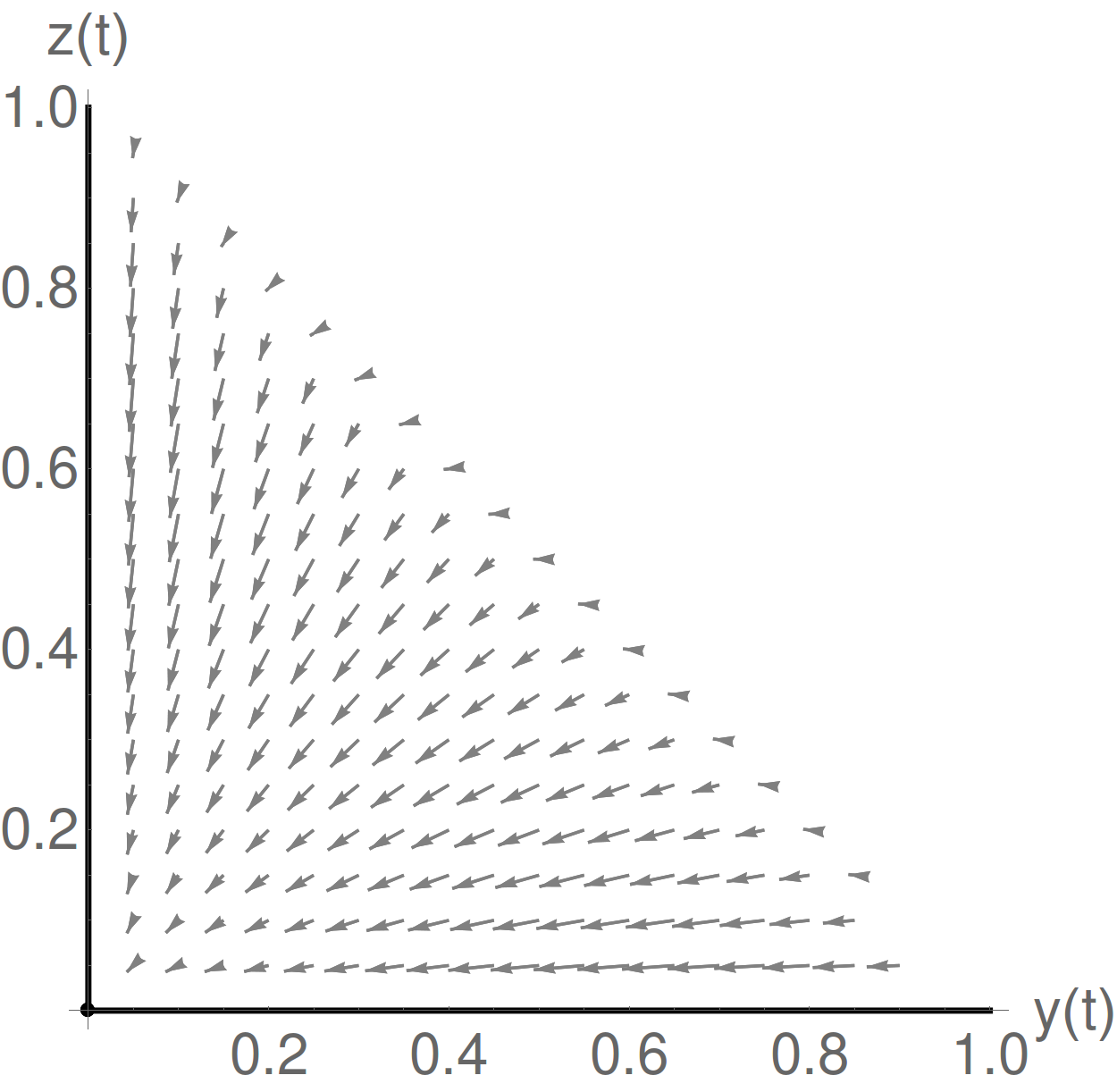
Figure 3: Numerical illustration of the RG flow at the “phase-space boundaries” for flavour invariants in the SM (2G, one-loop accuracy, neglecting electroweak gauge couplings). Top: $z\equiv 0$; center: $y\equiv 0$; bottom $x\equiv 0$. Each arrow indicates the RG flow from $t_{0}=0$ to $t=5$; the starting values are again chosen as $I_{1}(\mu_{0})=1.0$, $I_{2}(\mu_{0})=0.1$, $\alpha_{s}(\mu_{0})=0.2$. The plots on the left (right) are generated assuming $I_{5}(\mu_{0})=\mp\sqrt{I_{3}I_{4}-\widetilde{I}_{5}}(\mu_{0})$.

3 Three Quark Generations

For three quark generations in the SM, the flavour symmetry group to consider now is

$${\cal G}_{\rm quark} =U(3)^{3}/U(1)_{B}\sim SU(3)_{Q_{L}}\times U(3)_{U_{R}}\times U(3)_{D_{R}}\,.$$ (63)

The corresponding Yukawa matrices again transform as bi-doublets under a change of flavour basis,

$$Y_{U}\to V_{Q_{L}}Y_{U}V_{U_{R}}^{\dagger}\,,\qquad Y_{D}\to V_{Q_{L}}Y_{D}V_{D_{R}}^{\dagger}\,.$$

In a particular flavour basis, they are given by

$$Y_{U}=\left(\begin{array}[]{ccc}y_{u}&0&0\\ 0&y_{c}&0\\ 0&0&y_{t}\end{array}\right)\,,\qquad Y_{D}=V_{\rm CKM}\left(\begin{array}[]{ccc}y_{d}&0&0\\ 0&y_{s}&0\\ 0&0&y_{b}\end{array}\right)\,.$$ (70)

In the subsequent analysis, it turns out to be more convenient to discuss the flavour invariants as a function of the CKM elements $V_{ij}$ without choosing a particular parametrization in terms of mixing angles which would directly reflect the unitarity of the CKM matrix $V_{\rm CKM}$.

3.1 Flavour Invariants

As discussed in Jenkins:2009dy , the SM quark sector in the 3G case can be described in terms of $10+1$ polynomially independent invariants, which determine 6 Yukawa eigenvalues, 3 mixing angles and the cosine and sine of the CP-violating phase (in a given parametrization of the CKM matrix). With a similar procedure as in the 2G case, we will now explicitly construct a convenient set for these 11 invariants from the non-negative hermitian matrices,

$$U\equiv Y_{U}Y_{U}^{\dagger}\,,\qquad D\equiv Y_{D}Y_{D}^{\dagger}\,,$$

which now transform under the $SU(3)_{Q_{L}}$ flavour symmetry. For later use we also define the adjoint matrices, satisfying

$$U\,{\rm adj}\,U=\det U\quad\mbox{etc.}$$

With this, we can easily construct a complete set of polynomially independent positive semi-definite invariants. For the unmixed invariants, we define

$$I_{1} \equiv\text{tr}\left(U\right)\geq 0\,, I_{2}\equiv\text{tr}\left(D\right)\geq 0\,,$$ (71)

$$\widehat{I}_{3} \equiv\text{tr}\left({\rm adj}\,U\right)\geq 0\,, \widehat{I}_{4}\equiv\text{tr}\left({\rm adj}\,D\right)\geq 0\,,$$ (72)

$$\widehat{I}_{6} \equiv\det\left(U\right)\geq 0\,, \widehat{I}_{8}\equiv\det\left(D\right)\geq 0\,,\,.$$ (73)

These determine the six singular values of the Yukawa matrices. The CKM elements are then determined by mixed invariants which we define in a similar way. CP-even invariants can be chosen as

$$\widehat{I}_{5}\equiv\text{tr}\left(UD\right)\geq 0\,,\qquad\widehat{I}_{7}\equiv\text{tr}\left(D\,{\rm adj}\,U\right)\geq 0\,,\qquad\widehat{I}_{9}\equiv\text{tr}\left(U\,{\rm adj}\,D\right)\geq 0\,,$$ (74)

and

$$\widehat{I}_{10} \equiv\text{tr}\left({\rm adj}\,(UD)\right)\geq 0\,,$$ (75)

According to the discussion in Jenkins:2009dy , there is an eleventh, CP-odd, invariant that cannot be expressed as a polynomial of the other ten invariants, as defined above. It is related to the Jarlskog determinant Jarlskog:1985ht and can be chosen as

$$I_{11}^{-} =-\frac{3i}{8}\,\det\left[U,D\right]\,.$$ (76)

Explicit expression in terms of Yukawa couplings and CKM elements can be found in Appendix B.

Octet Matrices and Octet Invariants:

As in the 2G case, we can also construct basic flavour matrices as octet representations of the flavour group factor $SU(3)_{Q_{L}}$. First, there are two polynomially independent octet matrices that are quadratic in the Yukawas, namely the traceless part of the matrices $U$ and $D$ (defined analogously to the 2G case),

$$U_{8}\equiv U-\frac{1}{3}\,\text{tr}[U]\,\mathds{1}\,,\qquad D_{8}\equiv U-\frac{1}{3}\,\text{tr}[D]\,\mathds{1}\,.$$ (77)

For terms quartic in the Yukawas, we may define the octet part of the adjoint matrices,

$${\rm adj}\,U_{8}\equiv{\rm adj}\,U-\frac{1}{3}\,\text{tr}[{\rm adj}\,U]\,\mathds{1}\,,\qquad{\rm adj}\,D_{8}\equiv{\rm adj}\,D-\frac{1}{3}\,\text{tr}[{\rm adj}\,D]\,\mathds{1}\,,$$

together with

$$S_{8}\equiv\frac{1}{2}\left\{U,D\right\}-\frac{1}{3}\,\text{tr}[UD]\,\mathds{1}\,,\qquad A_{8}\equiv\frac{i}{2}\left[U,D\right]\,.$$ (78)

Similarly, we define

$$A_{U}\equiv\frac{i}{2}\left[{\rm adj}\,U,D\right]\,,\qquad A_{D}\equiv\frac{i}{2}\left[{\rm adj}\,D,U\right]\,.$$ (79)

$\text{tr}\left[\ \right]$	$U_{8}$	$D_{8}$	${\rm adj}\,U_{8}$	${\rm adj}\,D_{8}$	$S_{8}$	$A_{8}$	$A_{U}$	$A_{D}$
$U_{8}$	$I_{3}$	$I_{5}$	$I_{6}$	$I_{9}$	$\widetilde{I}_{7}$	0	0	0
$D_{8}$	+	$I_{4}$	$I_{7}$	$I_{8}$	$\widetilde{I}_{9}$	0	0	0
${\rm adj}\,U_{8}$	+	+	$P_{1}$	$P_{2}$	$P_{3}$	0	0	0
${\rm adj}\,D_{8}$	+	+	+	$P_{4}$	$P_{5}$	0	0	0
$S_{8}$	+	+	+	+	$I_{10}$	0	0	0
$A_{8}$	0	0	0	0	0	$\widetilde{I}_{10}$	$Q_{1}$	$Q_{2}$
$A_{U}$	0	0	0	0	0	+	$Q_{3}$	$Q_{4}$
$A_{D}$	0	0	0	0	0	+	+	$Q_{5}$

Table 2: Traces of basic octet matrices constructed from $Y_{U}Y_{U}^{\dagger}$ and $Y_{D}Y_{D}^{\dagger}$ as defined in the text.

For generic Yukawa entries, the eight hermitian matrices as defined above provide a basis for octet matrices in $SU(3)_{Q_{L}}$. The symmetric (but non-orthogonal) metric defined by the traces of matrix products contains flavour invariants for the $3\times 3$ case. It is summarized in Table 2. Here, the unhatted invariants are related to the hatted ones via

$$I_{3}\equiv\text{tr}[U_{8}^{2}] =\frac{2}{3}I_{1}^{2}-2\widehat{I}_{3}\,, I_{4}\equiv\text{tr}[D_{8}^{2}]=\frac{2}{3}I_{2}^{2}-2\widehat{I}_{4}\,,$$ (80)

$$I_{6}\equiv\text{tr}[U_{8}\,{\rm adj}\,U_{8}] =3\widehat{I}_{6}-\frac{I_{1}\widehat{I}_{3}}{3}\,, I_{8}\equiv\text{tr}[D_{8}\,{\rm adj}\,D_{8}]=3\widehat{I}_{8}-\frac{I_{2}\widehat{I}_{4}}{3}\,,$$ (81)

and

$$I_{5} \equiv\text{tr}[U_{8}D_{8}]=\widehat{I}_{5}-\frac{I_{1}I_{2}}{3}\,,$$ (82)

and

$$I_{7} \equiv\text{tr}[D_{8}\,{\rm adj}\,U_{8}]=\widehat{I}_{7}-\frac{I_{2}\widehat{I}_{3}}{3}\,,\qquad I_{9}\equiv\text{tr}[U_{8}\,{\rm adj}\,D_{8}]=\widehat{I}_{9}-\frac{I_{1}\widehat{I}_{4}}{3}\,,$$ (83)

and

$$\widetilde{I}_{7} \equiv\text{tr}[U_{8}S_{8}]=\widehat{I}_{7}-I_{2}\widehat{I}_{3}+\frac{2I_{1}\widehat{I}_{5}}{3}\,,$$ (84)

$$\widetilde{I}_{9} \equiv\text{tr}[D_{8}S_{8}]=\widehat{I}_{9}-I_{1}\widehat{I}_{4}+\frac{2I_{2}\widehat{I}_{5}}{3}\,,$$ (85)

Finally, one has

$$I_{10} \equiv\text{tr}[S_{8}S_{8}]=\frac{\widehat{I}_{3}\widehat{I}_{4}-\widehat{I}_{10}}{2}+\frac{(\widehat{I}_{5}-I_{1}I_{2})\,\widehat{I}_{5}}{6}+\frac{I_{1}\widetilde{I}_{9}+I_{2}\widetilde{I}_{7}}{2}\,.$$ (86)

Further polynomially dependent invariants that appear in Table 2 are given by

$$\widetilde{I}_{10} \equiv\text{tr}[A_{8}^{2}]=I_{10}+2\widehat{I}_{10}-\frac{2\widehat{I}_{5}^{2}}{3}\,,$$ (87)

and

$$P_{1}\equiv\text{tr}[{\rm adj}\,U_{8}\,{\rm adj}\,U_{8}] =-2I_{1}\widehat{I}_{6}+\frac{2\widehat{I}_{3}^{2}}{3}\,,\qquad P_{4}\equiv\text{tr}[{\rm adj}\,D_{8}\,{\rm adj}\,D_{8}]=-2I_{2}\widehat{I}_{8}+\frac{2\widehat{I}_{4}^{2}}{3}\,,$$ (88)

and

$$P_{2}\equiv\text{tr}[{\rm adj}\,U_{8}\,{\rm adj}\,D_{8}] =\widehat{I}_{10}-\frac{\widehat{I}_{3}\widehat{I}_{4}}{3}\,,$$ (89)

and

$$P_{3}\equiv\text{tr}[{\rm adj}\,U_{8}\,S_{8}] =I_{2}\widehat{I}_{6}-\frac{\widehat{I}_{3}\widehat{I}_{5}}{3}\,,\qquad P_{5}\equiv\text{tr}[{\rm adj}\,D_{8}\,S_{8}]=I_{1}\widehat{I}_{8}-\frac{\widehat{I}_{4}\widehat{I}_{5}}{3}\,.$$ (90)

Furthermore,

$$Q_{1} \equiv\text{tr}[A_{8}\,A_{U}]=-\frac{I_{1}\,(\widehat{I}_{10}-\widehat{I}_{3}\widehat{I}_{4})}{2}+\frac{3I_{4}\widehat{I}_{6}}{4}-\frac{\widehat{I}_{5}\widehat{I}_{7}}{2}-\frac{\widehat{I}_{3}\widehat{I}_{9}}{2}\,,$$ (91)

$$Q_{2} \equiv\text{tr}[A_{8}\,A_{D}]=+\frac{I_{2}\,(\widehat{I}_{10}-\widehat{I}_{3}\widehat{I}_{4})}{2}-\frac{3I_{3}\widehat{I}_{8}}{4}+\frac{\widehat{I}_{5}\widehat{I}_{9}}{2}+\frac{\widehat{I}_{4}\widehat{I}_{7}}{2}\,,$$ (92)

and

$$Q_{3} \equiv\text{tr}[A_{U}\,A_{U}]=\frac{\widehat{I}_{3}\,(\widehat{I}_{10}-\widehat{I}_{3}\widehat{I}_{4})}{2}+\frac{\widehat{I}_{6}\,(3I_{9}-I_{1}I_{4}+I_{2}I_{5})}{2}+\frac{(I_{2}\widehat{I}_{3}-\widehat{I}_{7})\,\widehat{I}_{7}}{2}\,,$$ (93)

$$Q_{5} \equiv\text{tr}[A_{D}\,A_{D}]=\frac{\widehat{I}_{4}\,(\widehat{I}_{10}-\widehat{I}_{3}\widehat{I}_{4})}{2}+\frac{\widehat{I}_{8}\,(3I_{7}-I_{2}I_{3}+I_{1}I_{5})}{2}+\frac{(I_{1}\widehat{I}_{4}-\widehat{I}_{9})\,\widehat{I}_{9}}{2}$$ (94)

and

$$Q_{4}\equiv\text{tr}[A_{U}\,A_{D}] =\frac{(\widehat{I}_{5}-I_{1}I_{2})(\widehat{I}_{10}-\widehat{I}_{3}\widehat{I}_{4})}{4}+\frac{(\widehat{I}_{7}-I_{2}\widehat{I}_{3})(\widehat{I}_{9}-I_{1}\widehat{I}_{4})}{4}$$ (95)

$$\quad-\frac{(\widehat{I}_{6}-I_{1}\widehat{I}_{3})(\widehat{I}_{8}-I_{2}\widehat{I}_{4})}{4}-2\widehat{I}_{6}\widehat{I}_{8}\,.$$ (96)

In order to project onto the eight basis matrices one needs the inverse of the metric in Table 2. The explicit result is rather lengthy and not very instructive, and we therefore refrain from quoting it here. We checked however that the metric is not singular for generic Yukawa entries.

3.2 One-Loop RG equations

In the 3G case, again, any flavour matrix that arises as a flavour-covariant product of SM Yukawa matrices $Y_{U}$ and $Y_{D}$ can be written as a linear combination of a finite set of basic matrices (constructed from $Y_{U}$ and $Y_{D}$) with coefficients given as polynomials of a finite number of flavour invariants (as a corollary to the discussion in Jenkins:2009dy ). The most general form of the RG equations then can be written as

$$\frac{dY_{U}}{d\ln\mu} =\left(a_{0}\,\mathds{1}+a_{1}\,U_{8}+a_{2}\,D_{8}+a_{3}\,{\rm adj}\,U_{8}+a_{4}\,{\rm adj}\,D_{8}+a_{5}\,S_{8}+ia_{6}\,A_{8}\right.$$ (97)

$$\qquad\left.+ia_{7}\,A_{U}+ia_{8}A_{D}\right)Y_{U}(\mu)\,,$$ (98)

$$\frac{dY_{D}}{d\ln\mu} =\left(b_{0}\,\mathds{1}+b_{1}\,D_{8}+b_{2}\,U_{8}+b_{3}\,{\rm adj}\,D_{8}+b_{4}\,{\rm adj}\,U_{8}+b_{5}\,S_{8}-ib_{6}\,A_{8}\right.$$ (99)

$$\qquad\left.-ib_{7}\,A_{D}-ib_{8}A_{U}\right)Y_{D}(\mu)\,,$$ (100)

As compared to the 2G case, the expressions for the RG equations of the flavour invariants derived from this general parametrization become rather lengthy. (The explicit structure of the two-loop expressions can be found in (167) in the appendix.)

3.2.1 General Form

If we restrict ourselves to the RG equations at one-loop accuracy. we can write

$$\frac{dY_{U}}{d\ln\mu} =\left(a_{0}\,\mathds{1}+a_{1}\,U_{8}+a_{2}\,D_{8}+\ldots\right)Y_{U}(\mu)\,,$$ (101)

$$\frac{dY_{D}}{d\ln\mu} =\left(b_{0}\,\mathds{1}+b_{1}\,D_{8}+b_{2}\,U_{8}+\ldots\right)Y_{D}(\mu)\,,$$ (102)

where the coefficients $a_{0},b_{0}$ are first-order polynomials of flavour invariants, and $a_{1,2},b_{1,2}$ are constant, see again Table 1. The RG equations for the quadratic invariants then take the same form as in the 2G-case,

$$\frac{dI_{1}}{dt} \simeq 2a_{0}\,I_{1}+2a_{1}\,I_{3}+2a_{2}\,I_{5}\,,\qquad\frac{dI_{2}}{dt}\simeq 2b_{0}\,I_{2}+2b_{1}\,I_{4}+2b_{2}\,I_{5}\,.$$ (103)

We remind the reader of the difference between the hatted and unhatted invariants, as defined in Section 3.1. For the remaining unmixed invariants, we also find simple expressions

$$\frac{d\widehat{I}_{3}}{dt} \simeq 4a_{0}\,\widehat{I}_{3}-2a_{1}\,I_{6}-2a_{2}\,I_{7}\,,\qquad\frac{d\widehat{I}_{4}}{dt}\simeq 4b_{0}\,\widehat{I}_{4}-2b_{1}\,I_{8}-2b_{2}\,I_{9}\,,$$ (104)

and

$$\frac{d\widehat{I}_{6}}{dt} =6a_{0}\,\widehat{I}_{6}\,,\qquad\frac{d\widehat{I}_{8}}{dt}=6b_{0}\,\widehat{I}_{8}\,.$$ (105)

Notice that the last two relations — with our convention in (100) where the coefficients $a_{i>0},b_{i>0}$ always multiply traceless matrices — are exact. The one-loop RG equations for the mixed invariants are determined as

$$\frac{d\widehat{I}_{5}}{dt} \simeq(2a_{0}+2b_{0})\,\widehat{I}_{5}+(2a_{1}+2b_{2})\,\widetilde{I}_{7}+(2a_{2}+2b_{1})\,\widetilde{I}_{9}\,,$$ (106)

together with

$$\frac{d\widehat{I}_{7}}{dt} =(4a_{0}+2b_{0})\,\widehat{I}_{7}+(2a_{1}-2b_{2})\left(\frac{I_{1}\widehat{I}_{7}}{3}-I_{2}\widehat{I}_{6}\right)$$ (107)

$$\quad-(2a_{2}-2b_{1})\left(\widehat{I}_{10}-\widehat{I}_{3}\widehat{I}_{4}+\frac{2I_{2}\widehat{I}_{7}}{3}\right)\,,$$ (108)

$$\frac{d\widehat{I}_{9}}{dt} =(4b_{0}+2a_{0})\,\widehat{I}_{9}+(2b_{1}-2a_{2})\left(\frac{I_{2}\widehat{I}_{9}}{3}-I_{1}\widehat{I}_{8}\right)$$ (109)

$$\quad-(2b_{2}-2a_{1})\left(\widehat{I}_{10}-\widehat{I}_{3}\widehat{I}_{4}+\frac{2I_{1}\widehat{I}_{9}}{3}\right)\,,$$ (110)

and

$$\frac{d\widehat{I}_{10}}{dt} =(4a_{0}+4b_{0})\,\widehat{I}_{10}+(2a_{1}+2b_{2})\left(\frac{I_{1}\widehat{I}_{10}}{3}-\widehat{I}_{4}\widehat{I}_{6}\right)+(2a_{2}+2b_{1})\left(\frac{I_{2}\widehat{I}_{10}}{3}-\widehat{I}_{3}\widehat{I}_{8}\right)\,.$$ (111)

The RG equations for the Jarlskog invariant is simple, and to one-loop accuracy reads

$$\frac{dI_{11}^{-}}{dt} =\left(6a_{0}+6b_{0}+2a_{1}\,I_{1}+2b_{1}\,I_{2}\right)I_{11}^{-}\,.$$ (112)

3.2.2 Exploiting Flavour Hierarchies

The RG equations again simplify when one exploits flavour hierarchies in the SM Yukawa matrices, which are also applicable to MFV extensions of the SM. For concreteness, we relate the scaling of the quark Yukawa couplings to the Wolfenstein parameter $\lambda$ in the CKM matrix, as it can be realized in Froggatt-Nielsen models Froggatt:1978nt (see also Feldmann:2006jk ; Feldmann:2009dc ), assuming

$$V_{12}\sim\lambda\,,\qquad V_{23}\sim\lambda^{2}\,,\qquad V_{13}\sim\lambda^{3}\,,\$$ (113)

and

$$y_{t}\sim\lambda^{0}\,,\quad y_{b}\sim\lambda^{2}\,,\quad y_{c}\sim\lambda^{3}\,,\quad y_{s}\sim\lambda^{6}\,,\quad y_{u,d}\sim\lambda^{8}\,.$$ (114)

Defining $\epsilon=\lambda^{2}$, the individual invariants scale as (see Appendix B)

$$I_{1}\simeq y_{t}^{2}\sim\epsilon^{0}\,,\qquad\widehat{I}_{3}\simeq y_{t}^{2}y_{c}^{2}\sim\epsilon^{3}\,,\qquad\widehat{I}_{6}=y_{t}^{2}y_{c}^{2}y_{u}^{2}\sim\epsilon^{11}\,,$$ (115)

$$I_{2}\simeq y_{b}^{2}\sim\epsilon^{2}\,,\qquad\widehat{I}_{4}\simeq y_{b}^{2}y_{s}^{2}\sim\epsilon^{8}\,,\qquad\widehat{I}_{8}=y_{b}^{2}y_{s}^{2}y_{d}^{2}\sim\epsilon^{16}\,,$$ (116)

and

$$\widehat{I}_{5}\simeq y_{t}^{2}y_{b}^{2}|V_{tb}|^{2}=I_{1}I_{2}+{\cal O}(\epsilon^{4})\,,\qquad \widehat{I}_{7}\simeq y_{t}^{2}y_{b}^{2}y_{c}^{2}|V_{ub}|^{2}\sim\epsilon^{8}\,,$$ (117)

$$\widehat{I}_{10}\simeq y_{t}^{2}y_{b}^{2}y_{c}^{2}y_{s}^{2}|V_{ud}|^{2}=\widehat{I}_{3}\widehat{I}_{4}+{\cal O}(\epsilon^{12})\,,\qquad \widehat{I}_{9}\simeq y_{t}^{2}y_{b}^{2}y_{s}^{2}|V_{td}|^{2}\sim\epsilon^{11}\,,$$ (118)

and

$$I_{11}^{-} \sim\epsilon^{16}\,.$$ (119)

The leading terms in the (one-loop) RG equations are then identified as

$$\frac{dI_{1}}{dt} \simeq\left(2a_{0}+\frac{4a_{1}}{3}\,I_{1}\right)I_{1}\,, \frac{dI_{2}}{dt}\simeq\left(2b_{0}+\frac{4b_{2}}{3}\,I_{1}\right)I_{2}\,,$$ (120)

$$\frac{d\widehat{I}_{3}}{dt} \simeq\left(4a_{0}+\frac{2a_{1}}{3}\,I_{1}\right)\widehat{I}_{3}\,, \frac{d\widehat{I}_{4}}{dt}\simeq\left(4b_{0}+\frac{2b_{2}}{3}\,I_{1}\right)\widehat{I}_{4}\,,$$ (121)

and

$$\frac{d(\widehat{I}_{5}-I_{1}I_{2})}{dt} \simeq\left(2a_{0}+2b_{0}+\frac{4a_{1}}{3}\,I_{1}-\frac{2b_{2}}{3}\,I_{1}\right)(\widehat{I}_{5}-I_{1}I_{2})\,,$$ (122)

and

$$\frac{d\widehat{I}_{6}}{dt} =6a_{0}\,\widehat{I}_{6}\,, \frac{d\widehat{I}_{7}}{dt}\simeq\left(4a_{0}+2b_{0}+\frac{2a_{1}-2b_{2}}{3}\,I_{1}\right)\widehat{I}_{7}\,,$$ (123)

$$\frac{d\widehat{I}_{8}}{dt} =6b_{0}\,\widehat{I}_{8}\,, \frac{d\widehat{I}_{9}}{dt}\simeq\left(4b_{0}+2a_{0}+\frac{4a_{1}-4b_{2}}{3}\,I_{1}\right)\widehat{I}_{9}\,,$$ (124)

and

$$\frac{d(\widehat{I}_{10}-\widehat{I}_{3}\widehat{I}_{4})}{dt} \simeq\left(4a_{0}+4b_{0}+\frac{2a_{1}+2b_{2}}{3}\,I_{1}\right)(\widehat{I}_{10}-\widehat{I}_{3}\widehat{I}_{4})\,.$$ (125)

together with

$$\frac{d\widehat{I}_{11}^{-}}{dt} \simeq\left(6a_{0}+6b_{0}+2a_{1}\,I_{1}\right)I_{11}^{-}\,.$$ (126)

As in the 2G example, only the coefficients $a_{0},b_{0},a_{1},b_{2}$ in (102) are needed in this approximation. Solving for the latter, one obtains

$$a_{0}\,dt=-\frac{dI_{1}}{6\,I_{1}}+\frac{d\widehat{I}_{3}}{3\,\widehat{I}_{3}}\,,\qquad a_{1}\,dt\simeq\frac{1}{2I_{1}}\left(2\,\frac{dI_{1}}{I_{1}}-\frac{d\widehat{I}_{3}}{\widehat{I}_{3}}\right)\,,$$ (127)

$$b_{0}\,dt=-\frac{dI_{2}}{6\,I_{2}}+\frac{d\widehat{I}_{4}}{3\,\widehat{I}_{4}}\,,\qquad b_{2}\,dt\simeq\frac{1}{2I_{1}}\left(2\,\frac{dI_{2}}{I_{2}}-\frac{d\widehat{I}_{4}}{\widehat{I}_{4}}\right)\,.$$ (128)

This leaves 7 relations that can be used to identify RG-invariant combinations of flavour invariants,

$$\frac{d\widehat{I}_{6}}{\widehat{I}_{6}}+\frac{dI_{1}}{I_{1}}=2\,\frac{d\widehat{I}_{3}}{\widehat{I}_{3}}\,,\qquad\frac{d\widehat{I}_{8}}{\widehat{I}_{8}}+\frac{dI_{2}}{I_{2}}\simeq 2\,\frac{d\widehat{I}_{4}}{\widehat{I}_{4}}\,,$$ (129)

and

$$\frac{d(\widehat{I}_{5}-I_{1}I_{2})}{\widehat{I}_{5}-I_{1}I_{2}}+\frac{dI_{2}}{I_{2}} \simeq\frac{dI_{1}}{I_{1}}+\frac{d\widehat{I}_{4}}{\widehat{I}_{4}}\,,$$ (130)

and

$$\frac{d\widehat{I}_{7}}{\widehat{I}_{7}}+\frac{dI_{2}}{I_{2}} \simeq\frac{d\widehat{I}_{3}}{\widehat{I}_{3}}+\frac{d\widehat{I}_{4}}{\widehat{I}_{4}}\,,\qquad\frac{d\widehat{I}_{9}}{\widehat{I}_{9}}+2\,\frac{dI_{2}}{I_{2}}\simeq\frac{dI_{1}}{I_{1}}+2\,\frac{d\widehat{I}_{4}}{\widehat{I}_{4}}\,,$$ (131)

and

$$\frac{d(\widehat{I}_{10}-\widehat{I}_{3}\widehat{I}_{4})}{\widehat{I}_{10}-\widehat{I}_{3}\widehat{I}_{4}} \simeq\frac{d\widehat{I}_{3}}{\widehat{I}_{3}}+\frac{d\widehat{I}_{4}}{\widehat{I}_{4}}\,,\qquad\frac{dI_{11}^{-}}{I_{11}^{-}}+\frac{dI_{2}}{I_{2}}\simeq\frac{dI_{1}}{I_{1}}+\frac{d\widehat{I}_{3}}{\widehat{I}_{3}}+2\,\frac{d\widehat{I}_{4}}{\widehat{I}_{4}}\,.$$ (132)

Here each of the invariants is to be read as a function of $(I_{1},I_{2},\widehat{I}_{3},\widehat{I}_{4})$. As in the 2G case, the relations can be easily integrated, resulting in

$$\frac{I_{1}\widehat{I}_{6}}{(\widehat{I}_{3})^{2}}\simeq\text{const.}\simeq\frac{y_{u}^{2}}{y_{c}^{2}}\sim\epsilon^{5}\,,\qquad\frac{I_{2}\widehat{I}_{8}}{(\widehat{I}_{4})^{2}}\simeq\text{const.}\simeq\frac{y_{d}^{2}}{y_{s}^{2}}\sim\epsilon^{2}\,,$$ (133)

and

$$\frac{I_{1}\widehat{I}_{4}}{I_{2}(\widehat{I}_{5}-I_{1}I_{2})}\simeq\text{const.}\simeq\frac{y_{s}^{2}}{y_{b}^{2}\,|V_{cb}|^{2}}\sim\epsilon^{2}\,,$$ (134)

and

$$\frac{\widehat{I}_{3}\widehat{I}_{4}}{I_{2}\widehat{I}_{7}}\simeq\text{const.}\simeq\frac{y_{s}^{2}}{y_{b}^{2}\,|V_{ub}|^{2}}\sim\epsilon\,,\qquad\frac{I_{1}\widehat{I}_{4}^{2}}{I_{2}\widehat{I}_{9}}\simeq\text{const.}\simeq\frac{y_{s}^{2}}{y_{b}^{2}\,|V_{td}|^{2}}\sim\epsilon\,,$$ (135)

and

$$\frac{\widehat{I}_{10}-\widehat{I}_{3}\widehat{I}_{4}}{\widehat{I}_{3}\widehat{I}_{4}}\simeq\text{const.}\simeq|V_{us}|^{2}\sim\epsilon\,,\qquad\frac{I_{1}\widehat{I}_{3}\widehat{I}_{4}}{I_{2}I_{11}^{-}}\simeq\text{const.}\simeq\frac{4y_{s}^{2}}{3y_{b}^{2}\,{\rm Im}[V_{ud}V_{ub}^{*}V_{td}^{*}V_{tb}]}\sim\epsilon\,.$$ (136)

This explicitly shows, how the known simplifications for the RG solutions of quark masses and mixing angles that arise in the limit of large top-quark Yukawa coupling (see also Liu:2009vh ) can be translated to the set of flavour invariants in a straightforward manner.

3.2.3 One-loop Solutions in the SM

As in the 2G-case, we can derive explicit solutions to the RG equations, using the one-loop expressions for the coefficients in Table 1 and the approximations from the Yukawa hierarchies discussed in the previous paragraph. With our definitions of flavour invariants, the approximate RG equations for the invariants $I_{1,2}$ and $\widehat{I}_{3,4}$ looks identical to the 2G case in (53,57,58). As a consequence, we can again express the running of the 11 invariants in terms of the RG function $G(\mu,\mu_{0})$ defined in (56) from the evolution of the leading invariant

$$I_{1}(\mu) \simeq\eta^{8/\beta_{0}}\,I_{1}(\mu_{0})\,G(\mu,\mu_{0})\,,\qquad\eta=\frac{\alpha_{s}(\mu)}{\alpha_{s}(\mu_{0})}\,.$$ (137)

Defining normalized invariants as before (using a slightly different notation), we have

$$x_{2}(\mu)\equiv\frac{I_{2}(\mu)}{I_{1}(\mu)} \simeq\left[G(\mu,\mu_{0})\right]^{-2/3}x_{2}(\mu_{0})\,,$$ (138)

$$x_{3}(\mu)\equiv\frac{\widehat{I}_{3}(\mu)}{(I_{1}(\mu))^{2}} \simeq\left[G(\mu,\mu_{0})\right]^{-1/3}x_{3}(\mu_{0})\,,$$ (139)

$$x_{4}(\mu)\equiv\frac{\widehat{I}_{4}(\mu)}{(I_{2}(\mu))^{2}} \simeq\left[G(\mu,\mu_{0})\right]^{+1/3}x_{4}(\mu_{0})\,.$$ (140)

and the remaining scaling relations follow from (133-136). In this way, we recover the results for the approximate RG running of CKM mixing angles as discussed in Balzereit:1998id .

Comparison with Harrison et al.

In a paper by Harrison et al. Harrison:2010mt it has been highlighted that, within the SM, the one-loop RG equations exhibit two combinations of flavour invariants that are stable with respect to RG flow,

$$\frac{d}{dt}\left(\frac{\text{tr}[UD]}{\left(\det[UD]\right)^{1/3}}\right)=\frac{d}{dt}\,\frac{\widehat{I}_{5}}{(\widehat{I}_{6}\widehat{I}_{8})^{1/3}} =0\qquad\mbox{(SM@1-loop)}\,,$$ (141)

$$\frac{d}{dt}\left(\text{tr}\left[(UD)^{-1}\right]\left(\det[UD]\right)^{1/3}\right)=\frac{d}{dt}\,\frac{\widehat{I}_{10}}{(\widehat{I}_{6}\widehat{I}_{8})^{2/3}} =0\qquad\mbox{(SM@1-loop)}\,.$$ (142)

In our notation, we have

$$\frac{d}{dt}\,\frac{\widehat{I}_{5}}{(\widehat{I}_{6}\widehat{I}_{8})^{1/3}} =\frac{2\,(a_{1}+b_{2})\,\widetilde{I}_{7}+2\,(a_{2}+b_{1})\,\widetilde{I}_{9}}{\left(\det[UD]\right)^{1/3}}\,,$$ (143)

$$\frac{d}{dt}\,\frac{\widehat{I}_{10}}{(\widehat{I}_{6}\widehat{I}_{8})^{2/3}} =\frac{2\,(a_{1}+b_{2})\left(I_{1}\widehat{I}_{10}-3\widehat{I}_{4}\widehat{I}_{6}\right)+2(a_{2}+b_{1})\left(I_{2}\widehat{I}_{10}-3\widehat{I}_{3}\widehat{I}_{8}\right)}{3\left(\det[UD]\right)^{2/3}}\,.$$ (144)

This indeed vanishes for $a_{1}=-b_{2}=-a_{2}=b_{1}$ which holds within the SM, see Table 1.

4 Summary and Outlook

From the experimental as well as form the theoretical side (see e.g. the reviews in Antonelli:2009ws ; Bediaga:2012py ; Buras:2013ooa ; Buras:2010wr ), the quark flavour physics program is currently entering the precision era. The goal is to find hints to physics beyond the Standard Model (SM) from dedicated experiments, notably LHCb and BELLE II. Still, the answer to the flavour puzzle itself may reside at extremely high scales, possibly as high as the Planck scale. In any case, the determination of flavour observables occurs at low energies, and thus for any comparison with “new physics” models one needs to include the renormalization-group (RG) running of the flavour parameters in a given theoretical framework. In principle, there are various roads to discuss this. On the one hand, one can consider the entries of the $3\times 3$ Yukawa matrices and study their RG evolution; but these depend on an arbitrary choice of basis in flavour space. Alternatively, one can use the physical parameters, i.e. the six quark masses together with four independent CKM parameters to describe quark mixing and CP violation in weak interactions; but these have rather complicated relations to the Yukawa couplings.

In this paper, we have chosen an intermediate point of view and considered simple combinations of Yukawa couplings that are independent of the orientation of the flavour basis. In terms of these flavour invariants we have formulated RG equations which are basis independent and allow for a transparent implementation of flavour hierarchies as observed in the SM or its minimal-flavour-violating (MFV) extensions. Expanding systematically in small parameters, we have also constructed simple analytic solutions for the RG evolution of a set of polynomially independent flavour invariants.

Discussing the RG flow in terms of flavour invariants may be advantageous to discuss models with dynamical flavour symmetry breaking, where the Yukawa couplings emerge as vacuum expectation values (VEVs) of some scalar flavon fields. The scalar potential generating these VEVs will be constructed in terms of polynomials of flavour invariants of a given canonical mass dimension. In MFV-like constructions (see e.g. Albrecht:2010xh ), these can be reduced to the set of invariants discussed in this work. More complicated situations arise if one implements the spontaneous breaking of a gauged flavour symmetry on the level of renormalizable interactions. This leads to an “inverted-MFV” scenario, where the fundamental flavour invariants are approximately given as polynomials of the inverse Yukawa matrices Grinstein:2010ve . Even more complicated relations can arise in a recently proposed model with dynamical flavour-symmetry breaking with a unification scheme according to Pati and Salam Feldmann:2015zwa . While the general form of the RG equations (100) will remain the same, the coefficients will have a more complicated dependence than in MFV scenarios. In any of these cases, the renormalization-group flow of the invariants is needed to constrain the theoretical NP parameters at a high scale from flavour observables at low scales, and eventually give us some clue on the solution of the flavour problem.

Appendix A Cayley-Hamilton Identities

A.1 Two-Generation Case

The Cayley-Hamilton identity for $2\times 2$ matrices $M$ reads

$$0 =M^{2}-\text{tr}[M]\,M+\det M\,\mathds{1}\,.$$ (145)

Taking the trace and solving for $\det M$, one obtains

$$\det M =\frac{1}{2}\left(\text{tr}^{2}[M]-\text{tr}[M^{2}]\right)\,.$$ (146)

Multiplying (145) with $M^{-1}$, and solving for ${\rm adj}\,M=M^{-1}\det M$, one obtains

$${\rm adj}\,M =\text{tr}[M]\,\mathds{1}-M\qquad\Rightarrow\qquad\text{tr}[{\rm adj}\,M]=\text{tr}[M]\,.$$ (147)

Inserted back into (145) yields

$$M^{2} =\text{tr}[M]\,M-\det[M]\,\mathds{1}\,.$$ (148)

For traceless matrices, this further simplifies to

$$M^{2} =\frac{1}{2}\,\text{tr}[M^{2}]\,\mathds{1}\qquad(\text{tr}[M]=0)\,.$$ (149)

Therefore any power of $2\times 2$ matrices $M$ can be reduced to the basis $\{\mathds{1},M\}$ with coefficients built from polynomials of $\text{tr}M$, $\text{tr}M^{2}$ which are invariant under unitary basis transformations.

For matrices $Y$ which transform under bi-unitary transformations, Eq. (147) generalizes to

$${\rm adj}\,Y =\frac{\det[Y]}{\det[M]}\,Y^{\dagger}\left(\text{tr}[M]\,\mathds{1}-M\right)\qquad\mbox{($M\equiv YY^{\dagger}$)}\,.$$ (150)

A.2 Three-Generation Case

The Cayley-Hamilton identity for $3\times 3$ matrices $M$ reads

$$0 =M^{3}-\text{tr}[M]\,M^{2}+\frac{1}{2}\left(\text{tr}^{2}[M]-\text{tr}[M^{2}]\right)M-\det M\,\mathds{1}\,.$$ (151)

Taking the trace and solving for $\det M$, one obtains

$$\det M =\frac{1}{3}\left(\text{tr}[M^{3}]-\frac{3}{2}\,\text{tr}[M]\text{tr}[M^{2}]+\frac{1}{2}\,\text{tr}^{3}[M]\right)\,.$$ (152)

Multiplying (151) with $M^{-1}$, and solving for ${\rm adj}\,M=M^{-1}\det M$, one obtains

$${\rm adj}\,M =M^{2}-\text{tr}[M]\,M+\frac{1}{2}\left(\text{tr}^{2}[M]-\text{tr}[M^{2}]\right)\mathds{1}$$ (153)

$$\Rightarrow\qquad\text{tr}[{\rm adj}\,M] =\frac{1}{2}\left(\text{tr}^{2}[M]-\text{tr}[M^{2}]\right)\,.$$ (154)

Inserted back into (151) yields

$$M^{3} =\text{tr}[M]\,M^{2}-\text{tr}[{\rm adj}\,M]\,M+\det[M]\,\mathds{1}\,.$$ (155)

For traceless matrices, this further simplifies to

$$M^{3} =\frac{1}{2}\,\text{tr}[M^{2}]\,M+\frac{1}{3}\,\text{tr}[M^{3}]\,\mathds{1}\qquad(\text{tr}[M]=0)\,.$$ (156)

Therefore any power of $3\times 3$ matrices $M$ can be reduced to the basis $\{\mathds{1},M,M^{2}\}$ with coefficients built from invariants that are polynomials of $\text{tr}M$, $\text{tr}M^{2}$, $\text{tr}M^{3}$.

Similarly as before, for matrices $Y$ which transform under bi-unitary transformations, Eq. (154) generalizes to

$${\rm adj}\,Y =\frac{\det[Y]}{\det[M]}\,Y^{\dagger}\left(\text{tr}[{\rm adj}\,M]\,\mathds{1}-\text{tr}[M]\,M+M^{2}\right)\qquad\mbox{($M\equiv YY^{\dagger}$)}\,.$$ (157)

Appendix B 3G Flavour Invariants, Yukawa Couplings and CKM Elements

For our convention to define 10+1 polynomially independent flavour invariants, the explicit expressions in terms of Yukawa couplings and mixing angles read as follows. The quadratic invariants are

$$I_{1} \equiv\text{tr}[U]=\sum_{i=u,c,t}y_{i}^{2}\,,\qquad I_{2}\equiv\text{tr}[D]=\sum_{j=d,s,b}y_{j}^{2}\,.$$ (158)

Again, $I_{1}$ and $I_{2}$ quantify the overall size of flavour-symmetry breaking in the up- and down-quark sector, respectively. Quartic invariants appear as

$$\widehat{I}_{3} \equiv\text{tr}[{\rm adj}\,U]=\sum_{i=u,c,t}\widetilde{y}_{i}^{2}\,,\qquad\widehat{I}_{4}\equiv\text{tr}[{\rm adj}\,D]=\sum_{j=d,s,b}\widetilde{y}_{j}^{2}\,,$$ (159)

and

$$\widehat{I}_{5} \equiv\text{tr}[UD]=\sum_{i=u,c,t}\sum_{j=d,s,b}y_{i}^{2}y_{j}^{2}\,|V_{ij}|^{2}\,,$$ (160)

where we have defined $\widetilde{y}_{u}^{2}=y_{c}^{2}y_{t}^{2}$, $\widetilde{y}_{d}^{2}=y_{s}^{2}y_{b}^{2}$ etc. Continuing with the sixth-order invariants, we have

$$\widehat{I}_{6} =\text{tr}[U\,{\rm adj}\,U]=3\det U=3\,y_{u}^{2}y_{c}^{2}y_{t}^{2}\,,\qquad\widehat{I}_{8}=\text{tr}[D\,{\rm adj}\,D]=3\det D=3\,y_{d}^{2}y_{s}^{2}y_{b}^{2}\,,$$ (161)

and

$$\widehat{I}_{7} \equiv\text{tr}[{\rm adj}\,U\,D]=\sum_{i=u,c,t}\sum_{j=d,s,b}\widetilde{y}_{i}^{2}y_{j}^{2}\,|V_{ij}|^{2}\,,$$ (162)

$$\widehat{I}_{9} \equiv\text{tr}[U\,{\rm adj}\,D]=\sum_{i=u,c,t}\sum_{j=d,s,b}y_{i}^{2}\widetilde{y}_{j}^{2}\,|V_{ij}|^{2}\,.$$ (163)

The eight-order invariant reads

$$\widehat{I}_{10}\equiv\text{tr}[{\rm adj}\,U\,{\rm adj}\,D]=\sum_{i=u,c,t}\sum_{j=d,s,b}\widetilde{y}_{i}^{2}\widetilde{y}_{j}^{2}\,|V_{ij}|^{2}\,.$$ (164)

Finally, the CP-odd invariant

$$I_{11}^{-} \equiv\text{tr}[A_{8}^{3}]=\frac{3}{4}\,(y_{t}^{2}-y_{c}^{2})(y_{t}^{2}-y_{u}^{2})(y_{c}^{2}-y_{u}^{2})(y_{b}^{2}-y_{s}^{2})(y_{b}^{2}-y_{d}^{2})(y_{s}^{2}-y_{d}^{2})\,{\rm Im}\left[V_{ud}V_{ub}^{*}V_{td}^{*}V_{tb}\right]\,,$$ (165)

is proportional to the Jarlskog determinant Jarlskog:1985ht .

Appendix C Two-Loop RG equations for 3G Flavour Invariants

The two-loop approximation for RG equations of the quark Yukawa matrices $Y_{U}$ and $Y_{D}$ in (100) is obtained by keeping factors that are at most quartic in the Yukawa couplings, i.e. neglecting the contributions with the flavour matrices $A_{U,D}$,

$$\frac{dY_{U}}{d\ln\mu} =\left(a_{0}\,\mathds{1}+a_{1}\,U_{8}+a_{2}\,D_{8}+a_{3}{\rm adj}\,U_{8}+a_{4}\,{\rm adj}\,D_{8}+a_{5}\,S_{8}+ia_{6}\,A_{8}+\ldots\right)Y_{U}(\mu)\,,$$ (166)

$$\frac{dY_{D}}{d\ln\mu} =\left(b_{0}\,\mathds{1}+b_{1}\,D_{8}+b_{2}\,U_{8}+b_{3}\,{\rm adj}\,D_{8}+b_{4}\,{\rm adj}\,U_{8}+b_{5}\,S_{8}-ib_{6}\,A_{8}+\ldots\right)Y_{D}(\mu)\,.$$ (167)

From this ansatz, it is straightforward – though tedious – to calculate the two-loop RG equations for the eleven flavour invariants. First, we have

$$\frac{dI_{1}}{dt} \simeq 2a_{0}\,I_{1}+2a_{1}\,I_{3}+2a_{2}\,I_{5}+2a_{3}\,I_{6}+2a_{4}\,I_{9}+2a_{5}\,\widetilde{I}_{7}\,,$$ (168)

$$\frac{dI_{2}}{dt} \simeq 2b_{0}\,I_{2}+2b_{1}\,I_{4}+2b_{2}\,I_{5}+2b_{3}\,I_{8}+2b_{4}\,I_{7}+2b_{5}\,\widetilde{I}_{9}\,,$$ (169)

where here and in the following the abbreviations for the combinations of flavour invariants are the same as in Table 2. Then

$$\frac{d\widehat{I}_{3}}{dt} \simeq 4a_{0}\,\widehat{I}_{3}-2a_{1}\,I_{6}-2a_{2}\,I_{7}-2a_{3}\,P_{1}-2a_{4}\,P_{2}-2a_{5}\,P_{3}\,,$$ (170)

$$\frac{d\widehat{I}_{4}}{dt} \simeq 4b_{0}\,\widehat{I}_{4}-2b_{1}\,I_{8}-2b_{2}\,I_{9}-2b_{3}\,P_{4}-2b_{4}\,P_{2}-2b_{5}\,P_{5}$$ (171)

and

$$\frac{d\widehat{I}_{6}}{dt} =6a_{0}\,\widehat{I}_{6}\,,\qquad\frac{d\widehat{I}_{8}}{dt}=6b_{0}\,\widehat{I}_{8}\,.$$ (172)

For the mixed invariants, one obtains

$$\frac{d\widehat{I}_{5}}{dt} \simeq(2a_{0}+2b_{0})\,\widehat{I}_{5}+(2a_{1}+2b_{2})\,\widetilde{I}_{7}+(2a_{2}+2b_{1})\,\widetilde{I}_{9}$$ (173)

$$\quad+(2a_{3}+2b_{4})\,P_{3}+(2a_{4}+2b_{3})\,P_{5}+(2a_{5}+2b_{5})\,I_{10}+(2a_{6}+2b_{6})\,\widetilde{I}_{10}\,,$$ (174)

and

$$\frac{d\widehat{I}_{7}}{dt} \simeq(4a_{0}+2b_{0})\,\widehat{I}_{7}+(2a_{1}-2b_{2})\left(\frac{I_{1}\widehat{I}_{7}}{3}-I_{2}\widehat{I}_{6}\right)-(2a_{2}-2b_{1})\left(\widehat{I}_{10}-\widehat{I}_{3}\widehat{I}_{4}+\frac{2I_{2}\widehat{I}_{7}}{3}\right)$$ (175)

$$\quad+(2a_{3}-2b_{4})\left(2\widehat{I}_{5}\widehat{I}_{6}-3I_{5}\widehat{I}_{6}-\frac{2\widehat{I}_{3}\widehat{I}_{7}}{3}\right)+(2a_{4}-2b_{3})\left(\frac{\widehat{I}_{4}\widehat{I}_{7}}{3}-\widehat{I}_{3}\widehat{I}_{8}\right)$$ (176)

$$\quad+(2a_{5}-2b_{5})\left((2\widehat{I}_{4}-I_{2}^{2})\,\widehat{I}_{6}+\frac{\widehat{I}_{5}\widehat{I}_{7}}{3}+Q_{1}\right)+(2a_{6}+2b_{6})\,Q_{1}\,,$$ (177)

$$\frac{d\widehat{I}_{9}}{dt} \simeq(2a_{0}+4b_{0})\,\widehat{I}_{9}-(2a_{2}-2b_{1})\left(\frac{I_{2}\widehat{I}_{9}}{3}-I_{1}\widehat{I}_{8}\right)-(2b_{2}-2a_{1})\left(\widehat{I}_{10}-\widehat{I}_{3}\widehat{I}_{4}+\frac{2I_{1}\widehat{I}_{9}}{3}\right)$$ (178)

$$\quad-(2a_{4}-2b_{3})\left(2\widehat{I}_{5}\widehat{I}_{8}-3I_{5}\widehat{I}_{8}-\frac{2\widehat{I}_{4}\widehat{I}_{9}}{3}\right)-(2a_{3}-2b_{4})\left(\frac{\widehat{I}_{3}\widehat{I}_{9}}{3}-\widehat{I}_{4}\widehat{I}_{6}\right)$$ (179)

$$\quad-(2a_{5}-2b_{5})\left((2\widehat{I}_{3}-I_{1}^{2})\,\widehat{I}_{8}+\frac{\widehat{I}_{5}\widehat{I}_{9}}{3}-Q_{2}\right)-(2a_{6}+2b_{6})\,Q_{2}\,,$$ (180)

and

$$\frac{d\widehat{I}_{10}}{dt} \simeq(4a_{0}+4b_{0})\,\widehat{I}_{10}+(2a_{1}+2b_{2})\left(\frac{I_{1}\widehat{I}_{10}}{3}-\widehat{I}_{4}\widehat{I}_{6}\right)+(2a_{2}+2b_{1})\left(\frac{I_{2}\widehat{I}_{10}}{3}-\widehat{I}_{3}\widehat{I}_{8}\right)$$ (181)

$$\quad-(2a_{3}+2b_{4})\left(\widehat{I}_{6}\,(\widehat{I}_{9}-I_{1}\widehat{I}_{4})+\frac{2\widehat{I}_{3}\widehat{I}_{10}}{3}\right)-(2a_{4}+2b_{3})\left((\widehat{I}_{7}-I_{2}\widehat{I}_{3})\,\widehat{I}_{8}+\frac{2\widehat{I}_{4}\widehat{I}_{10}}{3}\right)$$ (182)

$$\quad+(2a_{5}+2b_{5})\left(\frac{\widehat{I}_{5}\widehat{I}_{10}}{3}-3\widehat{I}_{6}\widehat{I}_{8}-Q_{4}\right)-(2a_{6}+2b_{6})\,Q_{4}\,.$$ (183)

and

$$\frac{dI_{11}^{-}}{dt} \simeq\left(6a_{0}+6b_{0}+2a_{1}I_{1}+2b_{2}I_{2}-2a_{4}\widehat{I}_{3}-2b_{4}\widehat{I}_{4}\right)I_{11}^{-}$$ (184)

$$\quad+\left((a_{5}+b_{5})\,\frac{\widehat{I}_{5}+I_{1}I_{2}}{2}-(a_{6}+b_{6})\,I_{5}\right)I_{11}^{-}\,.$$ (185)

References

• (1) M. E. Machacek and M. T. Vaughn, “Two Loop Renormalization Group Equations in a General Quantum Field Theory. 2. Yukawa Couplings,” Nucl. Phys. B 236 (1984) 221.
• (2) B. Grzadkowski and M. Lindner, “Nonlinear Evolution Of Yukawa Couplings,” Phys. Lett. B 193 (1987) 71. B. Grzadkowski, M. Lindner and S. Theisen, “Nonlinear Evolution Of Yukawa Couplings In The Double Higgs And Supersymmetric Extensions Of The Standard Model,” Phys. Lett. B 198 (1987) 64.
• (3) H. Arason, D. J. Castano, B. Keszthelyi, S. Mikaelian, E. J. Piard, P. Ramond and B. D. Wright, “Renormalization group study of the standard model and its extensions. 1. The Standard model,” Phys. Rev. D 46 (1992) 3945.
• (4) V. D. Barger, M. S. Berger and P. Ohmann, “Universal evolution of CKM matrix elements,” Phys. Rev. D 47 (1993) 2038 [hep-ph/9210260].
• (5) C. Balzereit, Th. Mannel and B. Plümper, “The Renormalization group evolution of the CKM matrix,” Eur. Phys. J. C 9 (1999) 197 [hep-ph/9810350].
• (6) C. R. Das and M. K. Parida, “New formulas and predictions for running fermion masses at higher scales in SM, 2 HDM, and MSSM,” Eur. Phys. J. C 20 (2001) 121 [hep-ph/0010004].
• (7) A. Crivellin and U. Nierste, “Supersymmetric renormalisation of the CKM matrix and new constraints on the squark mass matrices,” Phys. Rev. D 79 (2009) 035018 [arXiv:0810.1613 [hep-ph]].
• (8) E. E. Jenkins, A. V. Manohar and M. Trott, “Renormalization Group Evolution of the Standard Model Dimension Six Operators II: Yukawa Dependence,” JHEP 1401 (2014) 035 [arXiv:1310.4838 [hep-ph]].
• (9) A. V. Bednyakov, A. F. Pikelner and V. N. Velizhanin, “Three-loop SM beta-functions for matrix Yukawa couplings,” Phys. Lett. B 737 (2014) 129 [arXiv:1406.7171 [hep-ph]].
• (10) E. E. Jenkins and A. V. Manohar, “Algebraic Structure of Lepton and Quark Flavor Invariants and CP Violation,” JHEP 0910 (2009) 094 [arXiv:0907.4763 [hep-ph]].
• (11) G. Colangelo, E. Nikolidakis and C. Smith, “Supersymmetric models with minimal flavour violation and their running,” Eur. Phys. J. C 59 (2009) 75 [arXiv:0807.0801 [hep-ph]].
• (12) G. D’Ambrosio, G. F. Giudice, G. Isidori and A. Strumia, “Minimal flavor violation: An Effective field theory approach,” Nucl. Phys. B 645 (2002) 155 [hep-ph/0207036].
• (13) Th. Feldmann, M. Jung and T. Mannel, “Sequential Flavour Symmetry Breaking,” Phys. Rev. D 80 (2009) 033003 [arXiv:0906.1523 [hep-ph]].
• (14) R. Alonso, M. B. Gavela, L. Merlo and S. Rigolin, “On the scalar potential of minimal flavour violation,” JHEP 1107 (2011) 012 [arXiv:1103.2915 [hep-ph]].
• (15) E. Nardi, “Naturally large Yukawa hierarchies,” Phys. Rev. D 84 (2011) 036008 [arXiv:1105.1770 [hep-ph]].
• (16) J. R. Espinosa, C. S. Fong and E. Nardi, “Yukawa hierarchies from spontaneous breaking of the $SU(3)_{L}\times SU(3)_{R}$ flavour symmetry?,” JHEP 1302 (2013) 137 [arXiv:1211.6428 [hep-ph]].
• (17) C. S. Fong and E. Nardi, “Quark masses, mixings, and CP violation from spontaneous breaking of flavor $SU(3)^{3}$,” Phys. Rev. D 89 (2014) 3, 036008 [arXiv:1307.4412 [hep-ph]].
• (18) W. Buchmüller and D. Wyler, “Effective Lagrangian Analysis of New Interactions and Flavor Conservation,” Nucl. Phys. B 268 (1986) 621.
• (19) B. Grzadkowski, M. Iskrzynski, M. Misiak and J. Rosiek, “Dimension-Six Terms in the Standard Model Lagrangian,” JHEP 1010 (2010) 085 [arXiv:1008.4884 [hep-ph]].
• (20) T. Feldmann and T. Mannel, “Minimal Flavour Violation and Beyond,” JHEP 0702 (2007) 067 [hep-ph/0611095].
• (21) G. Isidori and D. M. Straub, “Minimal Flavour Violation and Beyond,” Eur. Phys. J. C 72 (2012) 2103 [arXiv:1202.0464 [hep-ph]].
• (22) S. R. Juarez Wysozka, H. Herrera, S.F., P. Kielanowski and G. Mora, “Scale dependence of the quark masses and mixings: Leading order,” Phys. Rev. D 66 (2002) 116007 [hep-ph/0206243].
• (23) T. Feldmann, T. Mannel and S. Schwertfeger, “Flavour Invariants and Residual Flavour Symmetries”, [in preparation].
• (24) R. Alonso, “Dynamical Yukawa Couplings,” arXiv:1307.1904 [hep-ph].
• (25) T. Feldmann and T. Mannel, “Large Top Mass and Non-Linear Representation of Flavour Symmetry,” Phys. Rev. Lett.  100 (2008) 171601 [arXiv:0801.1802 [hep-ph]].
• (26) A. L. Kagan, G. Perez, T. Volansky and J. Zupan, “General Minimal Flavor Violation,” Phys. Rev. D 80 (2009) 076002 [arXiv:0903.1794 [hep-ph]].
• (27) H. Fritzsch, “Quark Masses and Flavor Mixing,” Nucl. Phys. B 155 (1979) 189.
• (28) C. Jarlskog, “Commutator of the Quark Mass Matrices in the Standard Electroweak Model and a Measure of Maximal CP Violation,” Phys. Rev. Lett.  55 (1985) 1039.
• (29) C. D. Froggatt and H. B. Nielsen, “Hierarchy of Quark Masses, Cabibbo Angles and CP Violation,” Nucl. Phys. B 147 (1979) 277.
• (30) L. X. Liu, “Renormalization Invariants and Quark Flavor Mixings,” Int. J. Mod. Phys. A 25 (2010) 4975 [arXiv:0910.1326 [hep-ph]].
• (31) P. F. Harrison, R. Krishnan and W. G. Scott, “Exact One-Loop Evolution Invariants in the Standard Model,” Phys. Rev. D 82 (2010) 096004 [arXiv:1007.3810 [hep-ph]].
• (32) M. Antonelli, D. M. Asner, D. A. Bauer, T. G. Becher, M. Beneke, A. J. Bevan, M. Blanke and C. Bloise et al., “Flavor Physics in the Quark Sector,” Phys. Rept.  494 (2010) 197 [arXiv:0907.5386 [hep-ph]].
• (33) R. Aaij et al. [LHCb Collaboration], “Implications of LHCb measurements and future prospects,” Eur. Phys. J. C 73 (2013) 4, 2373 [arXiv:1208.3355 [hep-ex]].
• (34) A. J. Buras and J. Girrbach, “Towards the Identification of New Physics through Quark Flavour Violating Processes,” Rept. Prog. Phys.  77 (2014) 086201 [arXiv:1306.3775 [hep-ph]]. “BSM models facing the recent LHCb data: A First look,” Acta Phys. Polon. B 43 (2012) 1427 [arXiv:1204.5064 [hep-ph]].
• (35) A. J. Buras, “Minimal flavour violation and beyond: Towards a flavour code for short distance dynamics,” Acta Phys. Polon. B 41 (2010) 2487 [arXiv:1012.1447 [hep-ph]].
• (36) M. E. Albrecht, T. Feldmann and T. Mannel, “Goldstone Bosons in Effective Theories with Spontaneously Broken Flavour Symmetry,” JHEP 1010 (2010) 089 [arXiv:1002.4798 [hep-ph]].
• (37) B. Grinstein, M. Redi and G. Villadoro, “Low Scale Flavor Gauge Symmetries,” JHEP 1011 (2010) 067 [arXiv:1009.2049 [hep-ph]].
• (38) T. Feldmann, F. Hartmann, W. Kilian and C. Luhn, “Combining Pati-Salam and Flavour Symmetries,” arXiv:1506.00782 [hep-ph].