Quantum optics theory of electronic noise in coherent conductors

Abstract

We consider the electromagnetic field generated by a coherent conductor in which electron transport is described quantum mechanically. We obtain an input-output relation linking the quantum current in the conductor to the measured electromagnetic field. This allows us to compute the outcome of measurements on the field in terms of the statistical properties of the current. We moreover show how under ac-bias the conductor acts as a tunable medium for the field, allowing for the generation of single- and two-mode squeezing through fermionic reservoir engineering. These results explain the recently observed squeezing using normal tunnel junctions [G. Gasse et al., Phys. Rev. Lett. 111 136601 (2013); J.-C. Forgues et al., Phys. Rev. Lett.  114 130403 (2015)].

More than sixty years ago, Glauber showed that the electromagnetic radiation produced by a classical electrical current is itself classical Glauber (1951, 1963). The situation can however be different in mesoscopic conductors at low temperature. Indeed, in such conductors electron transport should no longer be considered classical and current is represented by an operator. Because this operator does not commute with itself when evaluated at different times or frequencies, Glauber’s results no longer apply. One may then wonder if a “quantum current” may generate a non-classical electromagnetic field. This is the central question addressed in this Letter: how does the quantum properties of current in a coherent conductor imprint on the properties of the electromagnetic field it radiates?

This question was partly addressed in Refs. Beenakker and Schomerus (2001, 2004); Lebedev et al. (2010) where it was shown, for example, that the statistics of photon emitted by a quantum conductor can deviate from the Poissonian statistics of a coherent state. While photon statistics is most naturally revealed by power detection, measurements on quantum conductors are more typically realized with linear (i.e. voltage) detectors revealing quadratures of the electromagnetic field radiated by the sample. As a result, Refs. Beenakker and Schomerus (2001, 2004); Lebedev et al. (2010) only partly answer the question.

More recently it was predicted that, under ac-bias, the electromagnetic field radiated by a coherent conductor can be squeezed Bednorz et al. (2013). The field is then characterized by fluctuations along one of two quadratures being smaller than the vacuum level. This prediction can be surprising since these quantum states of the electromagnetic field are usually associated with the presence of a nonlinear element, such as a Kerr medium in the optical frequency range Walls and Milburn (2008) or a Josephson junction at microwave frequencies Yurke et al. (1988). Nevertheless, squeezing was experimentally observed using a tunnel junction with linear current-voltage characteristics Gasse et al. (2013); Forgues et al. (2015). Here squeezing results from quantum shot noise of the junction under ac driving. The predictions of Ref. Bednorz et al. (2013) however only consider correlation functions of the current inside the conductor, not the properties of the emitted field that is squeezed and ultimately measured.

In this Letter, instead of focussing on the current in the coherent conductor, we determine the properties of the field that it radiates. We achieve this, using the langage of quantum optics, by deriving an input-output relation Yurke and Denker (1984); Yurke (2004); Collett and Gardiner (1984a) directly connecting the radiated electromagnetic field to the current. Given that currents and voltages in electrical circuits are nothing more than another representation of electromagnetic fields, the theoretical methods of quantum optics are particularly well suited. This relation allows us to compute expectation values of the field corresponding to various types of measurements on mesoscopic samples, including power detection and linear quadrature measurements. We then go a step further and consider the fermionic degrees of freedom of the conductor as a bath for the electromagnetic field of a microwave resonator. Tracing out the conductor’s degrees of freedom leads to a Lindblad master equation for the electromagnetic field in a squeezed bath and shows how the electrons in the coherent conductor act as an effective medium for the field. This provides clear insight into the incoherent mechanism responsible for squeezing of the field, as well as a way to compare this mechanism with conventional schemes based on coherent interactions with non-linearities.

Our first step is to model the electromagnetic environment of the sample as a semi-infinite transmission line of characteristic impedance $Z_{0}=\sqrt{L_{0}/C_{0}}$, with $L_{0}$ and $C_{0}$ the inductance and capacitance per unit length respectively. The position-dependent flux $\hat{\phi}_{\mathrm{tl}}(x,t)$ along the transmission line is Yurke and Denker (1984); Yurke (2004); Leppäkangas et al. (2013)

$$\hat{\phi}_{\mathrm{tl}}(x,t) = \alpha\int_{0}^{\infty}\frac{\mathrm{d}\omega}{\sqrt{\omega}}\left(\hat{a}_{\mathrm{in}}[\omega]e^{-i\omega(t+x/v)}\right.$$ (1)

$$\left.+\,\hat{a}_{\mathrm{out}}[\omega]e^{-i\omega(t-x/v)}+\mathrm{h.c.}\right),$$

where $v=1/\sqrt{L_{0}C_{0}}$ is the speed of light in the transmission line and $\alpha=\sqrt{\hbar Z_{0}/2}$ . The subscripts ‘$\mathrm{in}$’ and ‘$\mathrm{out}$’ denote components moving towards and away from the sample, respectively. The corresponding annihilation operators satisfy $[\hat{a}_{\mathrm{in}}[\omega],\hat{a}_{\mathrm{in}}^{\dagger}[\omega^{\prime}]]=2\pi\delta(\omega-\omega^{\prime})$ and similarly for $\hat{a}_{\mathrm{out}}$. Finally, current at position $x$ in the transmission line is given in terms of the flux by $\hat{I}_{\mathrm{tl}}(x,t)=L^{-1}_{0}\partial_{x}\hat{\phi}_{\mathrm{tl}}(x,t)$, while voltage is $\hat{V}_{\mathrm{tl}}(x,t)=\partial_{t}\hat{\phi}_{\mathrm{tl}}(x,t)$.

With the sample located at $x=0$, current conservation imposes that

$$\hat{I}_{\mathrm{s}}(t)=-\hat{I}_{\mathrm{tl}}(x=0,t),$$ (2)

where $\hat{I}_{\mathrm{s}}$ is the sample’s electron current operator in the presence of the transmission line and of classical voltage bias. This equality links the bosonic operators of the line to the fermionic degrees of freedom of the sample. In the frequency domain, this takes the form

$$\hat{a}_{\mathrm{out}}[\omega]=\hat{a}_{\mathrm{in}}[\omega]-i\sqrt{\frac{2Z_{0}}{\hbar\omega}}\hat{I}_{\mathrm{s}}[\omega]$$ (3)

which relates the field travelling away from the conductor $\hat{a}_{\mathrm{out}}$ to the incoming field $\hat{a}_{\mathrm{in}}$ and the condutor’s current operator $\hat{I}_{\mathrm{s}}$. This is akin to an input-output boundary condition in quantum optics Yurke and Denker (1984); Yurke (2004); Collett and Gardiner (1984b). An expression similar to Eq. (3) can be found in Ref. Beenakker and Schomerus (2001) for the case of a quantum conductor coupled to the electromagnetic field freely propagating in three dimensions.

Since $\hat{I}_{\mathrm{s}}[\omega]$ depends on the current evaluated at all times, it does not commute with $\hat{a}_{\mathrm{in}}[\omega]$. Care must therefore be taken when evaluating moments of $\hat{a}_{\mathrm{out}}[\omega]$. In Ref. Beenakker and Schomerus (2001), this problem was avoided by neglecting the influence of the field’s vacuum fluctuations on the current $\hat{I}_{\mathrm{s}}$. This is justified for a sample of impedance much larger than $Z_{0}$, thus very poorly matched to the transmission line, and does not correspond to usual experimental conditions where impedance matching is preferable. Here, we address the problem of non-commutativity by writing Eq. (3) in terms of the quantum conductor’s bare current operator $\hat{I}$ in the absence of the electromagnetic environment, rather than the full current $\hat{I}_{\mathrm{s}}$ containing the influence of the field. This is done by going to the Heisenberg picture and solving for the current operator perturbatively in the light-matter coupling $\alpha$. This linear response treatment is justified for typical low impedance electromagnetic environments such that $Z_{0}\ll R_{K}$ with $R_{K}=h/e^{2}\sim 26~{}\mathrm{k\Omega}$ the quantum of resistance. For the common experimental value $Z_{0}=50~{}\Omega$, one indeed has $e\alpha/\hbar=\sqrt{\pi Z_{0}/R_{K}}\sim 0.08\ll 1$. For low impedance sample and transmission line and when the sample can be treated in the lumped-element limit, we take the interaction between the line’s and samples’s degrees of freedom to be of the form $H_{\mathrm{I}}(t)=\hat{I}(t)\hat{\phi}_{\mathrm{tl}}(x=0,t)$ SM . To first order in $e\alpha/\hbar$ we then find Graham (1989)

$$\hat{I}_{\mathrm{s}}[\omega]=\hat{I}[\omega]+\hat{V}_{\mathrm{tl}}[\omega]/Z[\omega],$$ (4)

with $Z[\omega]$ the impedance of the sample. In this expression, $\hat{I}[\omega]$ is the Fourier transform of $\hat{I}(t)$, the electronic current operator evolving according to the bare quantum conductor Hamiltonian SM . In principle, this free Hamiltonian can contain disorder, interactions, etc., as well as the effect of the classical dc and ac bias voltage, $V_{\mathrm{dc}}+V_{\mathrm{ac}}\cos{\omega_{\mathrm{ac}}t}$, applied to the conductor.

Combining Eqs. (3) and (4) directly leads to

$$\hat{a}_{\mathrm{out}}[\omega]=r\hat{a}_{\mathrm{in}}[\omega]-it\frac{\hat{I}[\omega]}{\sqrt{2\hbar\omega Z^{-1}}},$$ (5)

with $r=\frac{Z-Z_{0}}{Z+Z_{0}}$ the reflection coefficient and $t=\frac{2\sqrt{ZZ_{0}}}{Z+Z_{0}}$ the transmission coefficient with $\left|r\right|^{2}+\left|t\right|^{2}=1$. In contrast to Eq. (3), the bare current operator $\hat{I}$ entering Eq. (5) commutes at all times with the incoming field $\hat{a}_{\mathrm{in}}$ that has not yet interacted with the conductor. Arbitrary correlation functions of the outgoing field can thus easily be evaluated with this input-output boundary condition.

As examples, we now discuss the results for different types of common measurements. For simplicity we restrict the discussion to the practically important case of an ideally matched sample, $Z[\omega]=R=Z_{0}$. Then $r=0$ and the outgoing field takes the simple form $\hat{a}_{\mathrm{out}}[\omega]=-i\hat{I}[\omega]/\sqrt{2S_{\text{vac}}(\omega)}$ where $S_{\text{vac}}(\omega)=\hbar\omega/R$ is the current noise spectral density of vacuum noise. Measurable properties of the output field are then fully determined by the current. In particular, second order moments of the output field are given in terms of current-current correlation functions which under ac excitation obey Gabelli and Reulet (2007, 2008); SM

$$\begin{split}\langle I[\omega^{\prime}]I[\omega]\rangle&=2\pi[\tilde{S}(\omega^{\prime})+S_{\text{vac}}(\omega^{\prime})]\delta(\omega^{\prime}+\omega)\\ &+2\pi\sum_{p\neq 0}X(\omega^{\prime})\delta(\omega^{\prime}+\omega-p\omega_{\mathrm{ac}}).\end{split}$$ (6)

In this expression,

$$\tilde{S}(\omega)=\sum_{n=-\infty}^{\infty}J^{2}_{n}\left(\frac{eV_{\mathrm{ac}}}{\hbar\omega_{\mathrm{ac}}}\right)S\left(V_{\mathrm{dc}}+\frac{n\hbar\omega_{\mathrm{ac}}}{e},\omega\right),$$ (7)

is the photo-assisted noise, $S(V,\omega)=F\left[S_{0}(V+\hbar\omega/e)+S_{0}(V-\hbar\omega/e)\right]/2+(1-F)S_{0}(\hbar\omega/e)$ the noise spectral density of current fluctuations in the conductor, $S_{0}(V)=R^{-1}eV\coth(eV/2k_{B}T)$ and $F$ the Fano factor Blanter and Büttiker (2000). Moreover,

$$\begin{split}X(\omega)&=\frac{F}{2}\sum_{n}J_{n}J_{n+p}\left[S_{0}\left(V_{\mathrm{dc}}+\frac{\hbar}{e}(\omega+n\omega_{\mathrm{ac}})\right)\right.\\ &\left.\quad+(-1)^{p}S_{0}\left(V_{\mathrm{dc}}-\frac{\hbar}{e}(\omega+n\omega_{\mathrm{ac}})\right)\right],\end{split}$$ (8)

characterizes the noise dynamics Gabelli and Reulet (2008). For brevity we have here omitted the argument of the Bessel functions $J_{n}$ that is the same as in Eq. (7).

We first consider photodetection of the output field in the experimentally relevant situation where the signal is band-pass filtered before detection. This can be taken into account by defining a filtered output field

$$\begin{split}\hat{b}_{\mathrm{out}}(t)&=\frac{1}{2\pi\sqrt{B}}\int_{B}\mathrm{d}\omega\,\mathrm{e}^{-i(\omega-\omega_{0})t}\hat{a}_{\mathrm{out}}[\omega],\end{split}$$ (9)

where $B$ refers to a measurement bandwidth centered at the observation frequency $\omega_{0}\gg 2\pi B$. With this definition, the filtered photo-current is SM

$$\langle\hat{b}_{\mathrm{out}}^{\dagger}(t)\hat{b}_{\mathrm{out}}(t)\rangle=\frac{\tilde{S}(\omega_{0})-S_{\text{vac}}(\omega_{0})}{2S_{\text{vac}}(\omega_{0})},$$ (10)

where we have assumed a small filter bandwidth and dropped terms rotating at $\omega_{\mathrm{ac}}$ or faster. As expected, a photodetector is sensitive to the spectral density of the current noise emitted by the conductor Lesovik and Loosen (1997); Gavish et al. (2000); Clerk et al. (2010). In practice, this can be measured by separating the emission and absorption noise Aguado and Kouwenhoven (2000); Deblock et al. (2003). A more common detection scheme is to measure the time-averaged power of the emitted electromagnetic field. Again assuming a small measurement bandwidth, we find from Eq. (1) that $\overline{\langle V(t)^{2}\rangle}/R=(2\pi)^{2}B\tilde{S}(\omega_{0})R$, where we have omitted a contribution from the vacuum noise of the in-field SM . In contrast to photodetection, measurement of the power of the electromagnetic field is related to the symmetric current-current correlator containing both emission and absorption Clerk et al. (2010). This is not in contradiction with the fact that a passive detector cannot detect vacuum fluctuations Gavish et al. (2000). Power measurements are indeed performed using active devices like amplifiers and mixers.

Following the experiments of Refs. Gasse et al. (2013); Forgues et al. (2015), we now consider measurement of field quadratures as obtained by homodyne detection Walls and Milburn (2008). Defining quadratures of the output field in the frequency domain as $\hat{X}_{\mathrm{out}}[\omega]=\hat{a}_{\mathrm{out}}^{\dagger}[\omega]+\hat{a}_{\mathrm{out}}[\omega]$ and $\hat{Y}_{\mathrm{out}}[\omega]=i(\hat{a}_{\mathrm{out}}^{\dagger}[\omega]-\hat{a}_{\mathrm{out}}[\omega])$, and using Eq. (5), we immediately find for the variance of these quantities SM

$$\begin{split}\Delta\hat{X}_{\mathrm{out}}^{2}[\omega]&=\frac{\langle\{\hat{I}[-\omega],\hat{I}[\omega]\}\rangle-2\langle\hat{I}[\omega]^{2}\rangle}{2S_{\text{vac}}(\omega)},\\ \Delta\hat{Y}_{\mathrm{out}}^{2}[\omega]&=\frac{\langle\{\hat{I}[-\omega],\hat{I}[\omega]\}\rangle+2\langle\hat{I}[\omega]^{2}\rangle}{2S_{\text{vac}}(\omega)}.\end{split}$$ (11)

In practice, $\langle I[\omega]^{2}\rangle$ is only non-zero in the presence of ac-bias on the sample. Indeed, as expressed by Eq. (6), modulation of the bias voltage at frequency $\omega_{\mathrm{ac}}$ induces correlations between Fourier components of the current separated by $p\omega_{\mathrm{ac}}$, with $p$ an integer Gabelli and Reulet (2007, 2008). For $p\omega_{\mathrm{ac}}=2\omega_{0}$, and defining filtered output quadratures, $\hat{X}_{\mathrm{out,f}}(t)=\hat{b}_{\mathrm{out}}^{\dagger}(t)+\hat{b}_{\mathrm{out}}(t)$ and $\hat{Y}_{\mathrm{out,f}}(t)=i[\hat{b}_{\mathrm{out}}^{\dagger}(t)-\hat{b}_{\mathrm{out}}(t)]$, we find SM

$$\begin{split}\Delta\hat{X}_{\mathrm{out,f}}^{2}(t)&=2\left(N(\omega_{0})+\frac{1}{2}-M(\omega_{0})\right),\\ \Delta\hat{Y}_{\mathrm{out,f}}^{2}(t)&=2\left(N(\omega_{0})+\frac{1}{2}+M(\omega_{0})\right),\end{split}$$ (12)

where

$$N(\omega)=\frac{\tilde{S}(\omega)-S_{\text{vac}}(\omega)}{2S_{\text{vac}}(\omega)},\quad M(\omega)=\frac{X(\omega)}{2S_{\text{vac}}(\omega)}.$$ (13)

Clearly, the $X$ quadrature of the output field is squeezed when $M(\omega_{0})>N(\omega_{0})$, equivalently $X(\omega_{0})>\tilde{S}(\omega_{0})-S_{\text{vac}}(\omega_{0})$, with $M(\omega)$ and $N(\omega)$ bounded from the Heisenberg inequality by $N(\omega)[N(\omega)+1]\geq M(\omega)^{2}$ Walls and Milburn (2008). The same condition for squeezing was found in Refs. Gasse et al. (2013); Bednorz et al. (2013) by directly postulating the link between the field quadratures and the current operator for a normal tunnel junction. The squeezing generated by such a junction is however moderate. At zero temperature we expect maximum squeezing of $\sim 2$ dB while the experiment of Ref. Gasse et al. (2013) reported squeezing of 1.3 dB.

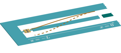
Figure 1: Transmission line resonator (blue) terminated by a normal tunnel junction. The first resonator mode envelope are illustrated for $R/Z_{0}=0.1$ (full brown line) and $R/Z_{0}=2000$ (dashed brown line). The output field can be measured via the capacitive coupling to the output port (dark blue).

To better understand the mechanism responsible for squeezing by the quantum conductor we now derive an equation of motion for the state $\rho(t)$ of the field. This is done by following the standard quantum optics approach: the bath is integrated out invoking the Born-Markov approximation to obtain a Lindblad master equation describing the dynamics of the field only Walls and Milburn (2008). The crucial difference from the usual treatment is that here the fermionic degrees of freedom of the sample play the role of bath for the bosonic modes of the field. Moreover, it is possible to engineer the system-bath interaction with the ac modulation frequency, leading to different field steady-states.

To simplify the discussion and because it is experimentally relevant Souquet et al. (2014); Altimiras et al. (2014); Parlavecchio et al. (2015), we consider the setup illustrated in Fig. 1 where a normal tunnel junction is fabricated at the end of a $\lambda/4$ transmission line-resonator of characteristic impedance $Z_{0}$. The case of a Josephson junction has been considered in Refs. Hofheinz et al. (2011); Leppäkangas et al. (2013); Gramich et al. (2013); Armour et al. (2013). The effect of the junction on the resonator is easily found by decomposing the resonator flux in terms of normal modes $\phi(x,t)=\sum_{m}\phi_{m}(t)u_{m}(x)$, with $u_{m}(x)$ the mode envelope SM ; Bourassa et al. (2012). The full line in Fig. 1 illustrates $|u_{1}(x)|$ for a junction impedance $R<Z_{0}$, while the dashed line corresponds to $u_{1}(x)$ for $Z_{0}>R$. As expected, in the former case the junction acts as a short to ground and the mode envelope approaches that of a $\lambda/4$ resonator, except for a small gap $|u_{1}(-L)|\sim R/Z_{0}$ at the location of the junction. On the other hand, for large tunnel resistance the junction acts as an open and the resonator’s bias on the junction is larger with $|u_{1}(-L)|\sim 1+(Z_{0}/R)^{2}$.

Having characterized the resonator mode in the presence of the junction, we now obtain the master equation assuming $Z_{0}\ll R_{K}$. In this limit, the interaction Hamiltonian reads $\hat{H}_{\mathrm{I}}=\sum_{m}\alpha_{m}\hat{I}(\hat{a}^{\dagger}_{m}+\hat{a}_{m})$, where $\alpha_{m}=\sqrt{\hbar Z_{m}}u_{m}(-L)$ with $Z_{m}$ the effective impedance of the resonator’s $m\mathrm{th}$ mode and $\hat{a}^{({\dagger})}_{m}$ the annihilation (creation) operator for the same mode SM . As above, the current operator $\hat{I}$ takes into account the presence of classical dc and ac bias on the junction.

We first focus on the situation where the ac frequency is, as above, $p\omega_{\mathrm{ac}}=2\omega_{m}$ where $p$ is an integer and $\omega_{m}$ now the frequency of the $m$th resonator mode. In the rotating-wave approximation we find SM

$$\begin{split}\dot{\rho}(t)&=\kappa_{m}(N_{m}+1)\mathcal{D}[\hat{a}_{m}]\rho+\kappa_{m}N_{m}\mathcal{D}[\hat{a}^{\dagger}_{m}]\rho\\ &+\kappa_{m}M_{m}\mathcal{S}[\hat{a}_{m}]\rho+\kappa_{m}M_{m}\mathcal{S}[\hat{a}^{\dagger}_{m}]\rho,\end{split}$$ (14)

with $\mathcal{D}[\hat{a}]\rho=\hat{a}\rho\hat{a}^{\dagger}-\{\hat{a}^{\dagger}\hat{a},\rho\}/2$ and $\mathcal{S}[X]\rho=\hat{a}\rho\hat{a}-\{\hat{a}^{2},\rho\}/2$. Eq. (14) is the standard master equation of a bosonic mode in a squeezed bath Walls and Milburn (2008) where $\kappa_{m}=u_{m}(-L)^{2}\omega_{m}Z_{m}/R$ is the cavity damping rate caused by the tunnel junction resistance . The thermal photon number $N_{m}=N(\omega_{m})$ and the quantity $M_{m}=M(\omega_{m})$ responsible for squeezing are the same as in Eq. (13). Evolution under Eq. (14) leads to steady-state variances of the intracavity quadratures $\hat{X}_{m}=\hat{a}^{\dagger}_{m}+\hat{a}_{m}$ and $\hat{Y}_{m}=i(\hat{a}^{\dagger}_{m}-\hat{a}_{m})$ taking the form $\Delta X_{m}^{2}=2N_{m}+1-2M_{m}$ and $\Delta Y_{m}^{2}=2N_{m}+1+2M_{m}$. In other words, intra-cavity squeezing is identical to what was found in Eq. (12) in the absence of the resonator.

The form of the above master equation clearly illustrates the dissipative nature of squeezing by a tunnel junction. This type of squeezing by dissipation has been explored theoretically in various systems and, in particular, in Ref. Didier et al. (2014) where it was shown that modulating the quality factor of a linear cavity could lead to ideal and unbounded squeezing. A similar mechanism is in action here with the periodic modulation of the Fermi level of the tunnel junction by the ac bias. The achievable squeezing is however neither pure nor unbounded, with the purity $p=S_{\mathrm{vac}}/\sqrt{\tilde{S}^{2}-X^{2}}<1$. At zero temperature, the highest expected purity is $p\sim 0.91$ corresponding to the 2 dB of squeezing mentioned above. This conclusion also applies to the cavity output field. Indeed, taking into account an output port (illustrated by the capacitor on the right-hand-side of Fig. 1) reduces intracavity squeezing by adding vacuum noise. This additional contribution is however absent from the cavity output field if the decay rates at the two ends of the resonator are matched Collett and Gardiner (1984a), leaving the degree of squeezing unchanged from the above input-output theory without cavity SM .

Taking advantage of the multi-mode structure of the resonator, other choices of ac drive can lead to entangled steady-states. In particular, taking $p\omega_{\mathrm{ac}}=\omega_{m}+\omega_{n}$ results in SM

$$\begin{split}\dot{\rho}(t)=&\sum_{l=n,m}\left\{\kappa_{l}(N_{l}+1)\mathcal{D}[\hat{a}_{l}]\rho+\kappa_{l}N_{l}\mathcal{D}[\hat{a}^{\dagger}_{l}]\rho\right\}\\ &+\sqrt{\kappa_{n}\kappa_{m}}M_{nm}\left(\hat{a}_{n}\rho\hat{a}_{m}+\hat{a}_{m}\rho\hat{a}_{n}+\{\hat{a}_{n}\hat{a}_{m},\rho\}\right)\\ &+\sqrt{\kappa_{n}\kappa_{m}}M_{nm}\left(\hat{a}^{\dagger}_{n}\rho\hat{a}^{\dagger}_{m}+\hat{a}^{\dagger}_{m}\rho\hat{a}^{\dagger}_{n}+\{\hat{a}^{\dagger}_{n}\hat{a}^{\dagger}_{m},\rho\}\right),\end{split}$$ (15)

where $\kappa_{l}$ and $N_{l}$ are the same as above and $M_{nm}=X(\omega_{n})/2\sqrt{S_{\text{vac}}(\omega_{n})S_{\text{vac}}(\omega_{m})}$. This master equation leads to two-mode squeezing. Indeed, in steady-state the variance of the joint quadratures $\hat{X}_{\pm}=\hat{X}_{n}\pm\hat{X}_{m}$ and $\hat{Y}_{\pm}=\hat{Y}_{n}\pm\hat{Y}_{m}$ are

$$\begin{split}\Delta X_{+}^{2}=\Delta Y_{-}^{2}=2(N_{n}+N_{m}+1-2M_{nm}),\\ \Delta X_{-}^{2}=\Delta Y_{+}^{2}=2(N_{n}+N_{m}+1+2M_{nm}),\end{split}$$ (16)

where we have assumed $\kappa_{n}=\kappa_{m}$ for simplicity. Similarly to the above single-mode case, the pairs of commuting quadratures $\Delta X_{+}^{2}$ and $\Delta Y_{-}^{2}$ are squeezed for $2M_{nm}>N_{n}+N_{m}$. It is interesting to point out that these quadratures are entangled when $\Delta X_{+}^{2}+\Delta Y_{-}^{2}<4$ Duan et al. (2000). This type of two-mode squeezing generated by a normal tunnel junction under the above ac modulation frequency was already experimentally reported in Ref. Forgues et al. (2015).

We finally consider the situation where the ac modulation is such that $p\omega_{\mathrm{ac}}=|\omega_{n}-\omega_{m}|$ in which case the master equation takes the form SM

$$\begin{split}\dot{\rho}(t)=&\sum_{l=n,m}\left\{\kappa_{l}(N_{l}+1)\mathcal{D}[\hat{a}_{l}]\rho+\kappa_{l}N_{l}\mathcal{D}[\hat{a}^{\dagger}_{l}]\rho\right\}\\ &+\sqrt{\kappa_{n}\kappa_{m}}M_{nm}\left(\hat{a}_{n}\rho\hat{a}^{\dagger}_{m}+\hat{a}^{\dagger}_{m}\rho\hat{a}_{n}-\{\hat{a}^{\dagger}_{m}\hat{a}_{n},\rho\}\right)\\ &+\sqrt{\kappa_{n}\kappa_{m}}M_{nm}\left(\hat{a}^{\dagger}_{n}\rho\hat{a}_{m}+\hat{a}_{m}\rho\hat{a}^{\dagger}_{n}-\{\hat{a}^{\dagger}_{n}\hat{a}_{m},\rho\}\right).\end{split}$$ (17)

Rather than two-mode squeezing, this describes correlated decay where emission by mode $n$ stimulates emission from mode $m$, and vice-versa. Under this evolution, the variance of the above joint quadratures keep the same form, except for $\Delta X_{+}^{2}$ and $\Delta X_{-}^{2}$ whose role are exchanged. Since $[\hat{X}_{-},\hat{Y}_{-}]=4i$, the variance of these two quadratures must respect $\Delta X_{-}\Delta Y_{-}\geq 2$ implying that $N_{n}+N_{m}\geq 2M_{nm}$. In other words, these quadratures cannot be squeezed below the vacuum level, also implying that the two modes are not entangled, and the master equation Eq. (17) only leads to squashing.

In summary, we have derived an input-output relation linking properties of the electrons in a quantum conductor to the measured electromagnetic field emitted by the conductor. We have also shown how the conductor act as a tunable medium for the field, allowing for the generation of single- and two-mode squeezing through fermionic reservoir engineering. Recent experimental observations of squeezing produced by a tunnel junction can be understood within this framework.

Note added. Recently, we became aware of an alternate description of squeezing by tunnel junction in a resonator Mendes and Mora (2015).

Acknowledgements– We thank Julien Gabelli and Karl Thibault for useful discussions. This work was supported by the Canada Excellence Research Chairs program, NSERC, FRQNT via INTRIQ and the Université de Sherbrooke via EPIQ.

See pages 1 of supmat See pages 2 of supmat See pages 3 of supmat See pages 4 of supmat See pages 5 of supmat See pages 6 of supmat See pages 7 of supmat See pages 8 of supmat See pages 9 of supmat

References

- Glauber (1951) R. J. Glauber, Phys. Rev. 84, 395 (1951).
- Glauber (1963) R. J. Glauber, Phys. Rev. 131, 2766 (1963).
- Beenakker and Schomerus (2001) C. W. J. Beenakker and H. Schomerus, Phys. Rev. Lett. 86, 700 (2001).
- Beenakker and Schomerus (2004) C. W. J. Beenakker and H. Schomerus, Phys. Rev. Lett. 93, 096801 (2004).
- Lebedev et al. (2010) A. V. Lebedev, G. B. Lesovik, and G. Blatter, Phys. Rev. B 81, 155421 (2010).
- Bednorz et al. (2013) A. Bednorz, C. Bruder, B. Reulet, and W. Belzig, Phys. Rev. Lett. 110, 250404 (2013).
- Walls and Milburn (2008) D. Walls and G. J. Milburn, Quantum Optics, 2nd ed. (Springer, Berlin, 2008).
- Yurke et al. (1988) B. Yurke, P. G. Kaminsky, R. E. Miller, E. A. Whittaker, A. D. Smith, A. H. Silver, and R. W. Simon, Phys. Rev. Lett. 60, 764 (1988).
- Gasse et al. (2013) G. Gasse, C. Lupien, and B. Reulet, Phys. Rev. Lett. 111, 136601 (2013).
- Forgues et al. (2015) J.-C. Forgues, C. Lupien, and B. Reulet, Phys. Rev. Lett. 114, 130403 (2015).
- Yurke and Denker (1984) B. Yurke and J. S. Denker, Phys. Rev. A 29, 1419 (1984).
- Yurke (2004) B. Yurke, “Quantum squeezing,” (Springer, 2004) Chap. 3.
- Collett and Gardiner (1984a) M. J. Collett and C. W. Gardiner, Phys. Rev. A 30, 1386 (1984a).
- Leppäkangas et al. (2013) J. Leppäkangas, G. Johansson, M. Marthaler, and M. Fogelström, Phys. Rev. Lett. 110, 267004 (2013).
- Note (1) We use the Fourier transform convention .
- Collett and Gardiner (1984b) M. J. Collett and C. W. Gardiner, Phys. Rev. A 30, 1386 (1984b).
- (17) See Supplemental Material for more information.
- Graham (1989) R. Graham, Zeitschrift für Physik B Condensed Matter 76, 265 (1989).
- Gabelli and Reulet (2007) J. Gabelli and B. Reulet, Proc. SPIE 6600, 66000T (2007).
- Gabelli and Reulet (2008) J. Gabelli and B. Reulet, ArXiv e-prints (2008), arXiv:0801.1432 .
- Blanter and Büttiker (2000) Y. Blanter and M. Büttiker, Physics Reports 336, 1 (2000).
- Gabelli and Reulet (2008) J. Gabelli and B. Reulet, Phys. Rev. Lett. 100, 026601 (2008).
- Lesovik and Loosen (1997) G. Lesovik and R. Loosen, Journal of Experimental and Theoretical Physics Letters 65, 295 (1997).
- Gavish et al. (2000) U. Gavish, Y. Levinson, and Y. Imry, Phys. Rev. B 62, R10637 (2000).
- Clerk et al. (2010) A. A. Clerk, M. H. Devoret, S. M. Girvin, F. Marquardt, and R. J. Schoelkopf, Rev. Mod. Phys. 82, 1155 (2010).
- Aguado and Kouwenhoven (2000) R. Aguado and L. P. Kouwenhoven, Phys. Rev. Lett. 84, 1986 (2000).
- Deblock et al. (2003) R. Deblock, E. Onac, L. Gurevich, and L. P. Kouwenhoven, Science 301, 203 (2003).
- Souquet et al. (2014) J. R. Souquet, M. J. Woolley, J. Gabelli, P. Simon, and A. A. Clerk, Nat Commun 5 (2014).
- Altimiras et al. (2014) C. Altimiras, O. Parlavecchio, P. Joyez, D. Vion, P. Roche, D. Esteve, and F. Portier, Phys. Rev. Lett. 112, 236803 (2014).
- Parlavecchio et al. (2015) O. Parlavecchio, C. Altimiras, J.-R. Souquet, P. Simon, I. Safi, P. Joyez, D. Vion, P. Roche, D. Esteve, and F. Portier, Phys. Rev. Lett. 114, 126801 (2015).
- Hofheinz et al. (2011) M. Hofheinz, F. Portier, Q. Baudouin, P. Joyez, D. Vion, P. Bertet, P. Roche, and D. Esteve, Phys. Rev. Lett. 106, 217005 (2011).
- Gramich et al. (2013) V. Gramich, B. Kubala, S. Rohrer, and J. Ankerhold, Phys. Rev. Lett. 111, 247002 (2013).
- Armour et al. (2013) A. D. Armour, M. P. Blencowe, E. Brahimi, and A. J. Rimberg, Phys. Rev. Lett. 111, 247001 (2013).
- Bourassa et al. (2012) J. Bourassa, F. Beaudoin, J. M. Gambetta, and A. Blais, Phys. Rev. A 86, 013814 (2012).
- Note (2) The Markov approximation is valid when the environment’s time scale is short with respect to Carmichael (1999) or in other words for . As expected, this implies that the sample resistance should not be matched to .
- Didier et al. (2014) N. Didier, F. Qassemi, and A. Blais, Phys. Rev. A 89, 013820 (2014).
- Duan et al. (2000) L.-M. Duan, G. Giedke, J. I. Cirac, and P. Zoller, Phys. Rev. Lett. 84, 2722 (2000).
- Mendes and Mora (2015) U. C. Mendes and C. Mora, ArXiv e-prints (2015), arXiv:1505.00031 .
- Carmichael (1999) H. J. Carmichael, Statistical Methods in Quantum Optics 1 (Springer, 1999).