Non-axisymmetric magnetic modes of neutron stars with purely poloidal magnetic fields

Abstract

We calculate non-axisymmetric oscillations of neutron stars magnetized by purely poloidal magnetic fields. We use polytropes of index $n=1$ and 1.5 as a background model, where we ignore the equilibrium deformation due to the magnetic field. Since separation of variables is not possible for the oscillation of magnetized stars, we employ finite series expansions for the perturbations using spherical harmonic functions. Solving the oscillation equations as the boundary and eigenvalue problem, we find two kinds of discrete magnetic modes, that is, stable (oscillatory) magnetic modes and unstable (monotonically growing) magnetic modes. For isentropic models, the frequency or the growth rate of the magnetic modes is exactly proportional to $B_{\rm S}$, the strength of the field at the surface. The oscillation frequency and the growth rate are affected by the buoyant force in the interior, and the stable stratification tends to stabilize the unstable magnetic modes.

1 Introduction

Neutron stars are believed to have strong magnetic fields. The field strength $B_{S}$ at the surface is estimated to be $\sim 10^{12}$ G for pulsars and $\sim 10^{15}$ G for magnetar candidates, but we do not have any good knowledge of the configuration of magnetic fields inside the star. Recently, quasi-periodic oscillations (QPOs) in the tail of the giant X/$\gamma$-ray flare were detected from the soft $\gamma$ ray repeaters (SGRs) (e.g., Israel et al. 2005; Strohmayer & Watts 2005). SGRs belong to what we call magnetars. Giant flares have so far been observed only from three SGRs, that is, SGR 0526-66, 1900+14, and 1806-20, and just once for each of the SGRs, indicating that giant flares in magnetars are quite rare events. The QPOs are now regarded as a manifestation of global oscillations of the underlying neutron stars, and it is expected that they can be used for seismological studies of the magnetars. However, it is not an easy task to properly carry out modal analysis of magnetar candidates because of their extremely strong magnetic fields, which can significantly modify the modal property of the stars. Because separation of variables between the radial and angular coordinates is not possible for the perturbations in magnetized stars, we have to employ series expansions to represent the perturbations in linear analysis, which possibly makes the analysis difficult, particularly when singular points inherent to the governing equations appear in the interior of the star (see, e.g., Asai, Lee, & Yoshida 2015).

Many authors have calculated axisymmetric ($m=0$) oscillation modes of magnetized stars having a purely poloidal magnetic field, where $m$ is the azimuthal wave number of modes. Using a toy model, Glampedakis, Samuelsson, and Andersson (2006) and Levin (2006, 2007) investigated global oscillation modes residing in the fluid core and in the solid crust both threaded by a magnetic field, and they showed that frequency resonance between modes in the core and in the crust could be important. Lee (2008) and Asai & Lee (2014) carried out normal mode calculations of axisymmetric toroidal modes and found discrete modes. van Hoven & Levin (2011, 2012) suggested the existence of discrete modes in the gaps between frequency continua, using spectral method. Besides the normal mode analyses mentioned above, however, most authors have used MHD simulations to investigate the modal properties of magnetized stars (e.g., Cerdá-Durán et al. 2009; Colaiuda & Kokkotas 2011; Gabler et al. 2011, 2012; Sotani et al. 2008). Sotani & Kokkotas (2009) calculated axisymmetric polar-Alfvén oscillations and found that continuous frequency spectra are not formed. Colaiuda & Kokkotas (2012) calculated mixed polar and axial oscillation modes of magnetized star having both poloidal and toroidal magnetic fields for axisymmetric perturbations. They suggested that the oscillation spectra can be significantly modified by the toroidal magnetic field component. Gabler et al. (2013a) calculated magnetic oscillation modes for various magnetic field configurations (e.g., purely poloidal, purely toroidal, mixed poloidal and toroidal).

For non-axisymmtric ($m\not=0$) modes of magnetized stars, however, there are only a few numerical studies of global oscillations. For purely toroidal magnetic field configuration, Lander et al. (2010), Passamonti & Lander (2013), and Asai, Lee, and Yoshida (2015) calculated non-axisymmetric oscillation modes. Lander & Jones (2011) calculated non-axisymmetric oscillation modes of magnetized rotating star with purely poloidal magnetic field using MHD simulations, and they obtained polar-led Alfvén modes, which reduce to inertial modes in the limit of ${\cal M}/{\cal T}\to 0$, where $\cal M$ and $\cal T$ are magnetic and rotation energies of the star. It is important to note that Lander & Jones (2011) suggested that the axial-led Alfvén modes could be unstable.

In this paper, employing the normal mode analysis, we calculate non-axisymmetric ($m\not=0$) oscillation modes of magnetized stars having purely poloidal magnetic fields. We assume that the gravitational energy dominates the magnetic energy so that the stellar deformation due to the magnetic field can be safely neglected. No effect of rotation is considered. For normal mode analysis in this paper, we employ finite series expansions for perturbed quantities to derive a finite set of coupled linear ordinary differential equations, which is solved as the boundary and eigenvalue problem by imposing appropriate boundary conditions. This paper is organized as follows. §2 describes the method used to construct a magnetized equilibrium stellar model, and perturbation equations for non-axisymmetric oscillation modes in magnetized stars are derived in §3. Numerical results are summarized in §4 and discussions about magnetic modes are summarized in §5. we conclude in §6. The details of the oscillation equations solved in this paper and suitable boundary conditions imposed at the stellar center and surface are given in Appendix.

2 Equilibrium model

Although we are concerned with magnetized neutron stars, in this study, we consider the problem within the frame work of Newtonian ideal magnetohydrodynamics for the sake of simplicity. For the modal analysis of magnetized stars composed of the infinitely conductive fluid, in this paper, magnetic fields in equilibrium are treated as perturbations about non-magnetized and non-rotating star. As mentioned before, we ignore the deformation of the star due to the magnetic stress and use self-gravitating polytropic spheres for the matter distribution of the star. Then, the mass density and pressure are given by

$$\rho=\rho_{0}\Theta^{n}\,,\quad p=p_{0}\Theta^{n+1}\,,$$ (1)

where $\rho_{0}$ and $p_{0}$ are the density and pressure values at the center of the star, respectively, and $n$ and $\Theta$ are the polytropic index and the Lane-Emden function, respectively. Imposed stationary axisymmetric magnetic fields are assumed to be the purely poloidal and dipole ones, given by

$$B_{r}=2f(r)\cos\theta,\quad B_{\theta}=-\left[r\dfrac{\mathrm{d}f(r)}{\mathrm{d}r}+2f(r)\right]\sin\theta,\quad B_{\phi}=0,$$ (2)

in which $\nabla\cdot\mbox{\boldmath$B$}=0$ is automatically satisfied. Here and henceforth, the spherical polar coordinate $(r,\theta,\phi)$ has been employed. The function $f(r)$ in Eq. (2) is determined by the Ampere law, $\nabla\times\mbox{\boldmath$B$}=4\pi j_{\phi}r\sin\theta\mbox{\boldmath$e$}_{\phi}$, which leads to

$$\dfrac{\mathrm{d}^{2}f}{\mathrm{d}r^{2}}+\frac{4}{r}\dfrac{\mathrm{d}f}{\mathrm{d}r}=-4\pi j_{\phi},$$ (3)

where $j_{\phi}$ is related to the toroidal current and needs to satisfy integrability conditions for the ideal magnetohydrodynamic (MHD) equations. In this study, we assume that $j_{\phi}=c_{0}\rho$ where $c_{0}$ is a constant determined by the boundary condition at the surface of the star. Near the center of the star, the function $f$ behaves as

$$f=\alpha_{0}+{\cal{O}}(r^{2}),$$ (4)

where $\alpha_{0}$ is a constant determined by the boundary condition at the surface of the star. We assume that $j_{\phi}=0$ outside the star. Thus, the exterior solution $f^{(\rm ex)}$ is given by $f^{(\rm ex)}=\mu_{b}/r^{3}$, where $\mu_{b}$ is the magnetic dipole moment of the star. We determine the constants $\alpha_{0}$ and $c_{0}$ so that the interior solutions $f$ and $\mathrm{d}f/\mathrm{d}r$ are continuously matched with the exterior solutions $f^{(\rm ex)}$ and $\mathrm{d}f^{(\rm ex)}/\mathrm{d}r$ at the surface of the star.

Figure 1: Magnetic field lines in the polytropic model of index $n=1$ (left panel) and $n=1.5$ (right panel).

The magnetic field lines in the polytropes of index $n=1$ and 1.5 are shown in Figure 1. We see that there exist field lines closed within the star.

3 Perturbation equations

The governing equations for non-radial oscillations of magnetized stars are obtained by linearizing the ideal MHD equations. Since the equilibrium state is stationary and axisymmetric, the time and azimuthal dependence of the perturbed quantities is given by the factor $\exp[i(\sigma t+m\phi)]$, where $m$ is the azimuthal wave number. The linearized basic equations that govern the adiabatic, non-radial oscillations of magnetized stars are written as

$$-\sigma^{2}\mbox{\boldmath$\xi$}=-\nabla\Phi^{\prime}-\frac{1}{\rho}\nabla p^{\prime}+\frac{\rho^{\prime}}{\rho^{2}}\dfrac{\mathrm{d}p}{\mathrm{d}r}\mbox{\boldmath$e$}_{r}+\frac{1}{4\pi\rho}\left[\left(\nabla\times\mbox{\boldmath$B$}^{\prime}\right)\times\mbox{\boldmath$B$}+\left(\nabla\times\mbox{\boldmath$B$}\right)\times\mbox{\boldmath$B$}^{\prime}\right],$$ (5)

$$\rho^{\prime}+\nabla\cdot\left(\rho\mbox{\boldmath$\xi$}\right)=0,$$ (6)

$$\frac{\rho^{\prime}}{\rho}=\frac{p^{\prime}}{\Gamma_{1}p}-\frac{\xi_{r}}{r}rA,$$ (7)

$$\mbox{\boldmath$B$}^{\prime}=\nabla\times\left(\mbox{\boldmath$\xi$}\times\mbox{\boldmath$B$}\right),$$ (8)

where $(^{\prime})$ indicates the Eulerian perturbation, and $rA$ in equation (7) denotes the Schwarzschild discriminant defined as

$$rA=\dfrac{\mathrm{d}\ln\rho}{\mathrm{d}\ln r}-\frac{1}{\Gamma_{1}}\dfrac{\mathrm{d}\ln p}{\mathrm{d}\ln r},$$ (9)

and $\Gamma_{1}=(\partial\ln p/\partial\ln\rho)_{\rm ad}$. For polytropes of the index $n$, the adiabatic exponent for the perturbations are assumed to be given by

$$\frac{1}{\Gamma_{1}}=\frac{n}{n+1}+\gamma$$ (10)

with $\gamma$ being a constant, for which $rA=-\gamma(\mathrm{d}\ln p/\mathrm{d}\ln r)\equiv\gamma V$. The star may be called radiative for $\gamma<0$, isentropic for $\gamma=0$, and convective for $\gamma>0$. For radiative stars, we have $g$-modes, whose oscillation frequency is proportional to $\sqrt{-\gamma}$. For simplicity, we employ the Cowling approximation, neglecting $\Phi^{\prime}$.

Because of the Lorentz force term in equation (5), separation of variables for the perturbations is impossible between the radial coordinate $r$ and the angular coordinate $\theta$. We therefore expand the perturbations in terms of the spherical harmonic functions $Y_{l}^{m}(\theta,\phi)$ with different $l$’s for a given azimuthal index $m$. The displacement vector $\xi$ is given by (see e.g., Lee 2005, 2007)

$$\xi_{r}=\sum_{j=1}^{j_{\rm max}}rS_{l_{j}}(r)Y_{l_{j}}^{m}(\theta,\phi),$$ (11)

$$\xi_{\theta}=\sum_{j=1}^{j_{\rm max}}\left[rH_{l_{j}}(r)\dfrac{\partial}{\partial\theta}Y_{l_{j}}^{m}(\theta,\phi)-irT_{l_{j}^{\prime}}(r)\frac{1}{\sin\theta}\dfrac{\partial}{\partial\phi}Y_{l_{j}^{\prime}}^{m}(\theta,\phi)\right],$$ (12)

$$\xi_{\phi}=\sum_{j=1}^{j_{\rm max}}\left[rH_{l_{j}}(r)\frac{1}{\sin\theta}\dfrac{\partial}{\partial\phi}Y_{l_{j}}^{m}(\theta,\phi)+irT_{l_{j}^{\prime}}(r)\dfrac{\partial}{\partial\theta}Y_{l_{j}^{\prime}}^{m}(\theta,\phi)\right],$$ (13)

and the vector $\mbox{\boldmath$B$}^{\prime}$ is given by

$$B_{r}^{\prime}=\sum_{j=1}^{j_{\rm max}}rb^{S}_{l_{j}^{\prime}}(r)Y_{l_{j}^{\prime}}^{m}(\theta,\phi),$$ (14)

$$B_{\theta}^{\prime}=\sum_{j=1}^{j_{\rm max}}\left[rb^{H}_{l_{j}^{\prime}}(r)\dfrac{\partial}{\partial\theta}Y_{l_{j}^{\prime}}^{m}(\theta,\phi)-irb^{T}_{l_{j}}(r)\frac{1}{\sin\theta}\dfrac{\partial}{\partial\phi}Y_{l_{j}}^{m}(\theta,\phi)\right],$$ (15)

$$B_{\phi}^{\prime}=\sum_{j=1}^{j_{\rm max}}\left[rb^{H}_{l_{j}^{\prime}}(r)\frac{1}{\sin\theta}\dfrac{\partial}{\partial\phi}Y_{l_{j}^{\prime}}^{m}(\theta,\phi)+irb^{T}_{l_{j}}(r)\dfrac{\partial}{\partial\theta}Y_{l_{j}}^{m}(\theta,\phi)\right],$$ (16)

where $l_{j}=|m|+2(j-1)$ and $l_{j}^{\prime}=l_{j}+1$ for even modes, and $l_{j}=|m|+2j-1$ and $l_{j}^{\prime}=l_{j}-1$ for odd modes, respectively, and $j=1,2,3,...,j_{\rm max}$. The Euler perturbations of the pressure and density are given by

$$p^{\prime}=\sum_{j=1}^{j_{\rm max}}p_{l_{j}}^{\prime}(r)Y_{l_{j}}^{m}(\theta,\phi),\quad\rho^{\prime}=\sum_{j=1}^{j_{\rm max}}\rho_{l_{j}}^{\prime}(r)Y_{l_{j}}^{m}(\theta,\phi).$$ (17)

For stars having a purely poloidal magnetic field, the oscillation modes are separated into even and odd modes. If the sets of the functions $(\xi_{r},\xi_{\phi},B^{\prime}_{\theta})$ and $(\xi_{\theta},B^{\prime}_{r},B^{\prime}_{\phi})$ of a mode are respectively even and odd (odd and even) functions about the equator, we call the mode an even (odd) mode. In this paper, we usually use $j_{\rm max}=12$ to obtain solutions with sufficiently high-angular resolution. Substituting the expansions (11)-(17) into the linearized basic equations (5) to (8), we obtain a finite set of coupled linear ordinary differential equations for the expansion coefficients $S_{l_{j}}(r)$, $T_{l_{j}^{\prime}}(r)$, $b^{S}_{l_{j}^{\prime}}(r)$, $b^{H}_{l_{j}^{\prime}}(r)$, $b^{T}_{l_{j}^{\prime}}(r)$, and $r\mathrm{d}b^{H}_{l_{j}^{\prime}}(r)/\mathrm{d}r$, which we call the oscillation equations to be solved in the interior of magnetized stars. The oscillation equations obtained for the star magnetized with a purely poloidal field are given in Appendix A. The set of ordinary differential equations is solved as an eigenvalue problem of $\sigma^{2}$ by applying boundary conditions at the center and surface of the star (see also Appendix A). Since the eigenvalue $\sigma^{2}$ is a real number for the boundary conditions we use, the eigenvalue $\sigma^{2}>0$ corresponds to stable and purely oscillatory modes of the frequency $\pm\sigma$, and $\sigma^{2}<0$ to unstable and monotonically growing modes of the growth rate $\eta=\sqrt{-\sigma^{2}}$.

For a given $j_{\rm max}$, we find numerous solutions to the oscillation equations. Most of them, however, are dependent on $j_{\rm max}$. We have to look for solutions that are independent of $j_{\rm max}$.

4 Numerical results

We use polytropes of index $n=1$ and 1.5 as a background model to calculate non-axisymmetric ($m\neq 0$) oscillations of stars magnetized with a poloidal field. In this numerical study, magnetic modes, the eigenvalue $\sigma^{2}$ of which is proportional to $B_{S}^{2}$, are only the modes we discuss. We cannot correctly compute $g$-, $f$-, and $p$-modes of the magnetized stars (see §6). We find both stable (oscillatory) magnetic modes with $\sigma^{2}>0$ and unstable (monotonically growing) magnetic modes with $\sigma^{2}<0$. In fact, if we write $\sigma=\sigma_{\rm I}\rm i=\pm\eta\rm i$ with $\eta$ being a positive real number, the time dependence of the modes is given by $\exp(\mp\eta t)$, and the modes with $\exp(\eta t)$ monotonically grow with time without bound where $\eta$ may be regarded as the growth rate. The modes with $\sigma^{2}<0$ may correspond to magnetic instability. It is well known that the stars having purely poloidal magnetic fields are unstable and the energy of the field is dissipated quickly, that is, for several ten milliseconds (e.g., Markey & Tayler 1973, van Assche, Goossens, Tayler 1982, Braithwaite 2007, Lasky et al. 2011; Ciolfi & Rezzolla 2012).

4.1 Stable Magnetic Modes

In Figure 2, we plot the eigenfrequencies $\sigma$ of stable magnetic modes that have no radial nodes of $S_{l_{1}}$ for $m=1$, 2, 3, and 4 versus the Alfvén frequency $\sigma_{A}$ defined as

$$\sigma_{A}\equiv B_{\rm S}/\sqrt{4\pi\rho_{c}R^{2}},$$ (18)

where $\rho_{c}$ is the central density, $R$ is the radius of the star, and $B_{\rm S}=\mu_{b}/R^{3}$ is the magnetic field strength measured at the surface, and the frequencies $\sigma$ and $\sigma_{A}$ are normalized by $\Omega_{\rm K}=\sqrt{GM/R^{3}}$ where $M$ is the mass of the star and $G$ is the gravitational constant. In this paper, we assume $M=1.4M_{\odot}$ and $R=10^{6}$cm, for which we have the ratio $\sigma_{A}/\Omega_{K}=4.42\times 10^{-4}(B_{S}/10^{15}{\rm G})$. In this paper we use the central density $\rho_{c}$ to define the Alfvén frequency $\sigma_{A}$. We may use instead the mean density $\bar{\rho}\equiv M/(4\pi R^{3}/3)$ for the definition. Since for polytropes $\bar{\rho}=-3\rho_{c}\zeta_{1}^{-1}\left(d{\Theta}/d{\zeta}\right)_{\zeta=\zeta_{1}}\equiv C\rho_{c},$ where $\Theta(\zeta)$ is the Lane-Emden function and $\Theta(\zeta_{1})=0$, we have $C=3/\pi^{2}\approx 0.304$ and 0.167 for the indices $n=1$ and 1.5. If we define $\sigma_{A}^{*}=B_{S}/\sqrt{4\pi\bar{\rho}R^{2}}$, we have $\sigma_{A}^{*}=\sigma_{A}/\sqrt{C}$. Note also that $\Omega_{K}=\sqrt{4\pi G\bar{\rho}/3}\propto\sqrt{G\bar{\rho}}$. We find that the eigenfrequency of the modes is isolated and proportional to the Alfvén frequency $\sigma_{A}$, that is, $B_{S}$. This property confirms that the modes we obtained are discrete magnetic modes.

Figure 2: Eigenfrequency $\sigma$ of the stable magnetic modes of odd parity for $m=1$, $2$, $3$, and $4$ versus the Alfvén frequency $\sigma_{A}$ for the $n=1$ polytrope.

Note that we find stable magnetic modes only for odd parity and cannot find stable magnetic modes of even parity.

In Table 1, we tabulate the eigenfrequency $\bar{\sigma}\equiv\sigma/\Omega_{K}$ of stable magnetic modes for the polytrope of index $n=1$ and 1.5 for $B_{\rm S}=10^{15}$ G. Here, we have assumed that $\gamma=0$. Note that the magnetic modes we can find for each value of $m$ are those that have only a few radial nodes of the expansion coefficient $S_{l}$, and it becomes difficult to find magnetic modes as the number of radial nodes increases. From Table 1, we find that for given $m$ and number of radial nodes, the normalized oscillation frequency $\bar{\sigma}$ of the magnetic mode of $n=1.5$ is larger than that of $n=1$. For a given $m$, the oscillation frequency gradually decreases as the number of radial nodes increases. This tendency of the oscillation frequency is similar to that found by Asai & Lee (2014) for axisymmetric ($m=0$) toroidal modes of the stars magnetized with a purely poloidal magnetic field in general relativistic framework. In addition, for a given number of radial nodes, the larger the azimuthal wavenumber $m$, the larger the frequency of the magnetic modes.

Table 1: Normalized eigenfrequency $\bar{\sigma}$ of the stable magnetic modes of odd parity for $B_{\rm S}=10^{15}$ G.

		$n=1$
$m$		number of radial nodes
	0	1	2
$1$	0.007523	0.007120	0.006954
$2$	0.007943	0.007464	0.007216
$3$	0.008174	0.007710	0.007439
$4$	0.008310	0.007887	0.007618
		$n=1.5$
$m$		number of radial nodes
	0	1	2
$1$	0.010304	0.009975	0.009817
$2$	0.010720	0.010247	0.010038
$3$	0.010961	0.010485	0.010229
$4$	0.011106	0.010663	0.010397

In Figure 3, we plot the eigenfunctions of an $m=1$ magnetic mode that has no radial nodes of $S_{l_{1}}$ for the $n=1$ polytrope and $B_{\rm S}=10^{15}$ G. We find that the eigenfunctions $S$, $H$, and $T$ of this mode have large amplitudes in the the core. We also find that the horizontal $H$ and toroidal $T$ components show rapid spacial oscillations near the stellar surface, although the radial component $S$ does not. This phenomena will be discussed in §5. Note that for isentropic ($\gamma=0$) models, we can obtain stable magnetic modes even for magnetic fields as weak as $B_{\rm S}\sim 10^{12}$ G.

Figure 3: Expansion coefficients $xS_{l}$, $xT_{l^{\prime}}$, and $xH_{l}$ as a function of $x=r/R$ for an $m=1$ stable magnetic mode of odd parity for the polytrope with $n=1$ for $B_{\rm S}=10^{15}$ G, where the solid lines, the long dashed lines, the short dashed lines, and the dotted lines are for the expansion coefficients associated with $l_{j}$ (or $l_{j}^{\prime}$) from $j=1$ to 4. The amplitude normalization is given by $T_{l^{\prime}_{l_{1}}}=1$ at the surface. Here, the frequency $\bar{\sigma}\equiv\sigma/\Omega_{\rm K}$ of the mode is 0.007523.

Assuming $\phi=0$, we may define the spacial oscillation pattern $\hat{\mbox{\boldmath$\xi$}}$ of the displacement vector $\xi$ as

$${\hat{\xi}}_{j}(r,\theta)=\xi_{j}(r,\theta,\phi=0),$$ (19)

where $j=r,~{}\theta,~{}\phi$, and the patterns $\hat{\xi}_{j}(r,\theta)$ for an $m=1$ stable magnetic mode are shown in Figure 4, where the vertical $z$-axis given by $x=0$ is the symmetry axis, and the amplitudes are normalized such that ${\rm max}(|\hat{\xi}_{j}(r,\theta)|)=1$ for $j=r,~{}\theta,~{}\phi$. Since the mode is an odd mode, as shown by the figure, the patterns $\hat{\xi}_{r}(r,\theta)$ and $\hat{\xi}_{\phi}(r,\theta)$ are antisymmetric about the equator given by $z=0$, while $\hat{\xi}_{\theta}(r,\theta)$ is symmetric. The oscillation patterns have large amplitudes along the symmetry axis. The $\phi$ component of $\hat{\mbox{\boldmath$\xi$}}$ shows a pattern that reflects the existence of magnetic fields closed within the interior.

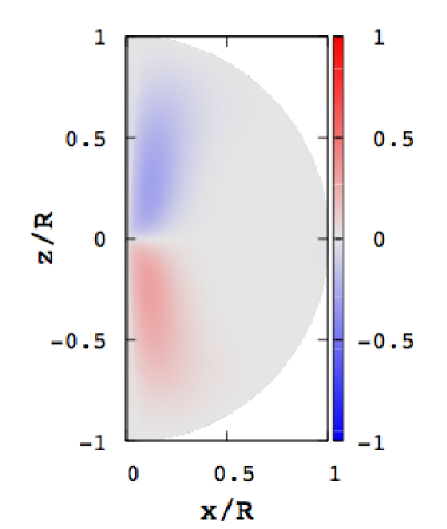
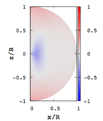
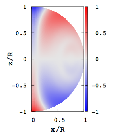
Figure 4: Spatial oscillation patterns $\hat{\xi}_{r}(r,\theta)$ (left), $\hat{\xi}_{\theta}(r,\theta)$ (middle), and $\hat{\xi}_{\phi}(r,\theta)$ (right) of the $m=1$ stable magnetic mode of Figure 3, where the amplitudes are normalized such that ${\rm max}(|\hat{\xi}_{j}(r,\theta)|)=1$.

In Table 2, we tabulate the ratios $|\hat{\xi}_{\theta}^{\rm max}|/|\hat{\xi}_{r}^{\rm max}|$ and $|\hat{\xi}_{\phi}^{\rm max}|/|\hat{\xi}_{r}^{\rm max}|$ for the nodeless magnetic modes of the $n=1$ and $n=1.5$ polytropes, where $|\hat{\xi}_{j}^{\rm max}|={\rm max}(|\hat{\xi}_{j}(r,\theta)|)$, and we have assumed $\gamma=0$ and $B_{\rm S}=10^{15}$ G. From Table 2, we find that the relative amplitudes $|\hat{\xi}_{\theta}^{\rm max}|/|\hat{\xi}_{r}^{\rm max}|$ and $|\hat{\xi}_{\phi}^{\rm max}|/|\hat{\xi}_{r}^{\rm max}|$ are rather insensitive to the azimuthal wavenumber $m$, and that the components $\hat{\xi}_{r}$ and $\hat{\xi}_{\theta}$ dominate $\hat{\xi}_{\phi}$. The pressure perturbation $\delta U\equiv p^{\prime}(r,\theta,\phi=0)/\rho gr$ has almost negligible amplitudes compared to the displacement vector. The oscillation patterns of the nodeless mode are almost the same for the $n=1$ and $n=1.5$ polytropes although the ratios $|\hat{\xi}_{\theta}^{\rm max}|/|\hat{\xi}_{r}^{\rm max}|$ and $|\hat{\xi}_{\phi}^{\rm max}|/|\hat{\xi}_{r}^{\rm max}|$ for $n=1$ are slightly larger than those for $n=1.5$ as indicated by Table 2. For the magnetic modes that have non-zero radial nodes of $S_{l_{1}}$, the tendencies of the amplitude ratios are found similar to those for the nodeless magnetic modes, and the oscillation patterns look quite similar for the polytropes of $n=1$ and 1.5

As $|m|$ increases, the oscillation amplitudes tend to be confined in the envelope region away from the symmetry axis, as exemplified by the spatial oscillation patterns of an $m=5$ unstable magnetic mode shown in Figure 8.

Table 2: Amplitude ratios between the components of the displacement vector of stable magnetic modes of odd parity for $B_{\rm S}=10^{15}$ G

		$n=1$
$m$	$|\hat{\xi}_{\theta}^{\rm max}|/|\hat{\xi}_{r}^{\rm max}|$	$|\hat{\xi}_{\phi}^{\rm max}|/|\hat{\xi}_{r}^{\rm max}|$	$|\delta U^{\rm max}|/|\hat{\xi}_{r}^{\rm max}|$
$1$	1.109	0.322	9.833$\times 10^{-6}$
$2$	0.787	0.304	1.236$\times 10^{-5}$
$3$	1.234	0.366	1.408$\times 10^{-5}$
$4$	1.121	0.396	1.595$\times 10^{-5}$
		$n=1.5$
$1$	2.552	0.111	6.954$\times 10^{-6}$
$2$	0.897	0.047	3.358$\times 10^{-6}$
$3$	1.124	0.051	5.376$\times 10^{-6}$
$4$	1.365	0.103	7.191$\times 10^{-6}$

4.2 Unstable Magnetic Modes

Table 3: Growth rate $\bar{\eta}\equiv\eta/\Omega_{\rm{K}}$ of the monotonically growing magnetic modes of even and odd parities for $B_{\rm{S}}=10^{15}$ G

				$n=1$
		even parity				odd parity
$m$		number of radial nodes		$m$		number of radial nodes
	1	2	3		1	2	3
1	0.000961	0.000580	0.000405	1
2	0.001557	0.000977	0.000709	2	0.003562
3	0.001964	0.001273	0.000949	3	0.004435	0.002038
4	0.002260	0.001505	0.001144	4	0.004879	0.003088
5	0.002488	0.001695	0.001452	5	0.005147	0.003685	0.002008
6	0.002676	0.001859	0.001452	6	0.005326	0.004086	0.002728
7	0.002852	0.002110	0.001889	7	0.005454	0.004377	0.003209
8	0.003096	0.002616	0.002069	8	0.005548	0.004598	0.003566
				$n=1.5$
		even parity				odd parity
$m$		number of radial nodes		$m$		number of radial nodes
	1	2	3		1	2	3
1	0.000898	0.000430		1
2	0.001601	0.000804		2
3	0.002114	0.001121		3
4	0.002482	0.001386		4	0.006170	0.003683
5	0.002769	0.001618		5	0.006510	0.004506	0.002007
6	0.003328	0.002611		6	0.006734	0.005047	0.003147
7	0.004089	0.002895		7	0.006892	0.005435	0.003849
8	0.004659	0.003053		8	0.007009	0.005727	0.004354

Unstable magnetic modes are found both for even parity and for odd parity. If we define the growth rate $\eta>0$ such that $\sigma=\pm\eta\rm i$, $\eta$ is almost exactly proportional to the field strength $B_{\rm S}$, particularly for the case of isentropic $(\gamma=0)$ models. In Table 3, we tabulate the normalized growth rate $\bar{\eta}\equiv\eta/\Omega_{\rm K}$ of unstable magnetic modes for the polytropes of index $n=1$ and 1.5, where we have assumed $\gamma=0$ and $B_{\rm S}=10^{15}$ G. Note that unstable magnetic modes are found even for magnetic fields as weak as $B_{\rm S}\sim 10^{12}$ G. From Table 3, we find that the growth rates $\bar{\eta}$ of the unstable magnetic modes for the $n=1$ and $n=1.5$ polytropes are quite similar, and that it becomes difficult to obtain unstable magnetic modes as the number of radial nodes increases, particularly for $n=1.5$. Between $m=1$ and $m=8$, we find unstable magnetic modes of odd parity only for $m\geq 2$ for $n=1$ and for $m\geq 4$ for $n=1.5$. For a given $m$, the growth rate $\bar{\eta}$ gradually decreases as the number of radial nodes of $S_{l_{1}}$ increases. On the other hand, for a given number of radial nodes, the larger the azimuthal index $m$, the larger the growth rate of the unstable modes. Using the normalized growth rate $\bar{\eta}$, the growth time scale $\tau_{g}=1/\eta$ may be given by

$$\tau_{g}=7.33\times 10^{-5}/\bar{\eta}\quad{\rm sec},$$ (20)

where we have assumed $M=1.4M_{\odot}$ and $R=10^{6}$cm. For a typical value of $\bar{\eta}\sim 10^{-3}$, the growth time scale may be $\tau_{g}\sim 5\times 10^{-2}$sec, which is consistent with the results, e.g., by Lasky et al. (2011) and Ciolfi & Rezzolla (2012).

Figure 5 shows the eigenfunctions of an $m=1$ unstable magnetic mode of even parity that has one radial node of $S_{l_{1}}$ for the $n=1$ polytrope for $B_{\rm S}=10^{15}$ G, where the amplitudes are normalized by $T_{l^{\prime}_{1}}=1$ at the surface. We find that $S_{l_{1}}$ has large amplitudes in the core, while $T_{l^{\prime}_{1}}$ in the envelope. The function $H_{l_{1}}$ has large amplitudes both in the core and in the envelope of the star. Note that the first components of $S$, $T$, and $H$ are dominating the other components.

Figure 5: Same as Figure 3 but for an $m=1$ unstable magnetic mode of even parity with the growth rate $\bar{\eta}=0.00096$.

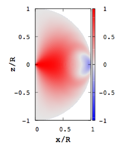
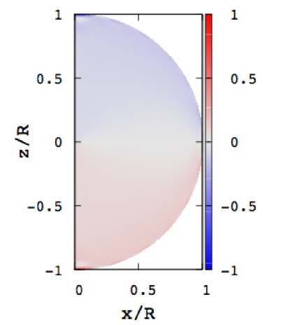
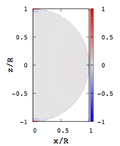
Figure 6: Same as Figure 4 but for the $m=1$ unstable magnetic mode of Figure 5.

The oscillation patterns $\hat{\xi}_{r}(r,\theta)$, $\hat{\xi}_{\theta}(r,\theta)$, and $\hat{\xi}_{\phi}(r,\theta)$ for the $m=1$ unstable magnetic mode are given in Figure 6. Since this mode has even parity, $\hat{\xi}_{r}$ and $\hat{\xi}_{\phi}$ are symmetric about the equator, while $\hat{\xi}_{\theta}$ is antisymmetric. The patterns $\hat{\xi}_{r}$ has large amplitudes along the equator, but the amplitudes of the $\theta$ and $\phi$ components of $\hat{\mbox{\boldmath$\xi$}}$ are confined to the polar regions. The existence of closed magnetic fields is recognized in the oscillation pattern of $\hat{\xi}_{r}$.

In Table 4, the ratios $|\hat{\xi}_{\theta}^{\rm max}|/|\hat{\xi}_{r}^{\rm max}|$ and $|\hat{\xi}_{\phi}^{\rm max}|/|\hat{\xi}_{r}^{\rm max}|$ are tabulated for the unstable magnetic modes of the $n=1$ and $n=1.5$ polytropes for $B_{\rm S}=10^{15}$ G. From Table 4, we find that relative amplitudes $|\hat{\xi}_{\theta}^{\rm max}|/|\hat{\xi}_{r}^{\rm max}|$ and $|\hat{\xi}_{\phi}^{\rm max}|/|\hat{\xi}_{r}^{\rm max}|$ decrease with the azimuthal wavenumber $m$, and that $\hat{\xi}_{\phi}$ dominates the other components. The pressure perturbation $\delta U$ have negligible amplitudes compared to the displacement vector as in the case of stable magnetic modes. The oscillation patterns are almost the same for the $n=1$ and $n=1.5$ polytropes.

Table 4: Amplitude ratios between the components of the displacement vector of the unstable magnetic modes of even parity for $B_{\rm S}=10^{15}$ G

		$n=1$
$m$	$|\hat{\xi}_{\theta}^{\rm max}|/|\hat{\xi}_{r}^{\rm max}|$	$|\hat{\xi}_{\phi}^{\rm max}|/|\hat{\xi}_{r}^{\rm max}|$	$|\delta U^{\rm max}|/|\hat{\xi}_{r}^{\rm max}|$
$1$	17.05	319.1	3.462$\times 10^{-4}$
$2$	10.95	120.5	3.706$\times 10^{-4}$
$3$	9.183	72.64	3.137$\times 10^{-4}$
$4$	7.996	49.24	2.538$\times 10^{-4}$
		$n=1.5$
$1$	31.98	685.1	1.471$\times 10^{-4}$
$2$	14.39	159.9	1.166$\times 10^{-4}$
$3$	7.662	63.72	7.266$\times 10^{-5}$
$4$	10.66	69.91	1.082$\times 10^{-4}$

Figures 7 and 8 show the eigenfunctions and spatial oscillation patterns of an $m=5$ unstable magnetic mode of odd parity that has one radial node of $S_{l_{1}}$ for the $n=1$ polytrope for $B_{\rm S}=10^{15}$ G. The toroidal components $T_{l_{j}}$ of the displacement vector $\xi$ look similar to those of the $m=1$ unstable mode of even parity in Figure 5, but the amplitudes of $S_{l_{j}}$ and $H_{l_{j}}$ are confined in the envelope region, in contast to those of the $m=1$ magnetic mode. This amplitude confinement to the envelope region is clearly seen in the spatial oscillation patterns shown in Figure 8. It is also interesting to note that the mode has negligible amplitudes along the symmetry axis.

Figure 7: Same as Figure 3 but for an $m=5$ oscillatory magnetic modes of odd parity with the growth rate $\bar{\eta}=0.005147$.

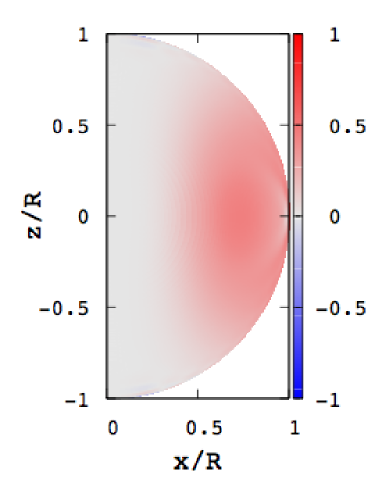
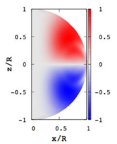
Figure 8: Same as Figure 4 but for the $m=5$ unstable magnetic mode of Figure 7.

5 Discussion

Magnetic modes depend on $\gamma$ as shown by Figure 9, in which the frequency $\sigma$ of a stable $m=2$ magnetic mode of odd parity with no radial nodes of $S_{l_{1}}$ and the growth rate $\eta/\sigma_{A}$ of an unstable $m=2$ magnetic mode of even parity are plotted as a function of $\sqrt{|\gamma|}$ for the $n=1$ polytrope and for $B_{\rm S}=10^{15}$ G. As $|\gamma|$ increases, the frequency $\sigma$ gradually increases (decreases) for $\gamma<0$ (for $\gamma>0$), and we find no magnetic mode for $\sqrt{|\gamma|}/\sigma_{A}\ga 10$. On the other hand, the growth rate $\eta$ decreases (increases) as $|\gamma|$ increases for $\gamma<0$ ($\gamma>0$), and we find no unstable solutions beyond $\sqrt{|\gamma|}/\sigma_{A}\ga 4$. For radiative stars with $\gamma<0$, the buoyant force tends to stabilize the magnetic instability. It is important to note that when we normalize the eigenvalue $\sigma$ (or $\eta$) and the Brunt-Väisälä frequency $N\propto\sqrt{|\gamma|}$ in terms of $\sigma_{A}$, the relation between $\sigma/\sigma_{A}$ (or $\eta/\sigma_{A}$) and $|\gamma|^{1/2}/\sigma_{A}$ in Figure 9 is almost independent of the magnetic field strength $B_{S}$.

Figure 9: Eigenfrequency $\sigma/\sigma_{A}$ (left) and the growth rate $\eta/\sigma_{A}$ (right) of the $m=2$ magnetic modes versus the $|\gamma|^{1/2}/\sigma_{A}$ for the $n=1$ polytrope.

Using a dispersion relation derived by Lee (2010) for the oscillation of magnetized stars, we try to explain the rapid spatial oscillations of the expansion coefficients $H$ and $T$ in the surface layers for stable magnetic modes. For a non-rotating and isentropic star, the dispersion relation may be given by

$$-pq^{2}\cos^{4}\alpha\left(Rk\right)^{6}+q^{2}\cos^{2}\alpha\left(2{p\over q}+1\right)\bar{\sigma}^{2}\left(Rk\right)^{4}+q\left[\bar{\beta}^{2}\cos^{2}\alpha-\left({p\over q}+1+\cos^{2}\alpha\right)\sigma^{2}\right]\bar{\sigma}^{2}\left(Rk\right)^{2}$$

$$+\bar{\sigma}^{2}\left[\bar{\sigma}^{4}-\bar{\sigma}^{2}\bar{\beta}^{2}+q\left(Rk_{H}\right)^{2}\bar{\beta}^{2}\sin^{2}\psi\right]=0,$$ (21)

where

$$p={a^{2}\over(R\Omega_{K})^{2}},\quad q={B^{2}/4\pi\rho\over(R\Omega_{K})^{2}},\quad\bar{\beta}^{2}={g^{2}/a^{2}\over\Omega_{K}^{2}},\quad a^{2}=\Gamma_{1}{p\over\rho},\quad g={GM_{r}\over r^{2}},\quad\cos\alpha={\mbox{\boldmath$k$}\cdot\mbox{\boldmath$B$}\over kB},\quad\sin\psi={(\mbox{\boldmath$k$}\times\mbox{\boldmath$B$})_{z}\over k_{H}B_{H}},$$ (22)

and $k=|\mbox{\boldmath$k$}|$ and $B=|\mbox{\boldmath$B$}|$. When we employ local cartesian coordinates $(x,y,z)$ and assume that the $z$-, $x$-, and $y$-directions at a point in the interior are respectively along the $r$-, $\theta$-, and $\phi$-directions at that point, we have $B_{z}=2f\cos\theta$, $B_{y}=0$, $B_{x}=-(2f+df/d\ln r)\sin\theta$, $k_{H}=\sqrt{k_{x}^{2}+k_{y}^{2}}$, $B_{H}=|B_{x}|$, and $\sin\psi=-k_{y}B_{x}/k_{H}|B_{x}|$. Assuming a polytrope of index $n=1$ with the mass $M=1.4M_{\odot}$ and the radius $R=10^{6}$cm and the field strength $B_{S}=10^{15}$G, we can compute the quantities $p$, $q$, $\bar{\beta}^{2}$, $a^{2}$, $g$ as a function of $r$. If we further assume for simplicity $k_{x}R=k_{y}R=1$ for $|m|\sim l\sim 1$ in the surface regions, we may solve equation (21) for $(Rk)^{2}$ to obtain $(Rk_{z})^{2}$ for given values of $\bar{\sigma}^{2}$, $\cos\theta$, and $\cos\alpha$. Figure 10 shows the local wavelengths $\lambda/R=2\pi/(Rk_{z})$ computed using the largest positive solution $(Rk_{z})^{2}$ in the outer envelope for several sets of parameters $(\bar{\sigma}^{2},\cos\theta,\cos\alpha)$. As shown by the figure, the waves propagating across the field lines, which may be provided by the closed field lines near the surface, tend to have short wavelengths, which become even shorter toward the surface. The wavelengths of the rapid spatial oscillations of the functions $H$ and $T$ near the surface become comparable to those expected for the case of $\cos\alpha\sim 0.01$. For low frequency modes we may expect $\mbox{\boldmath$k$}\cdot\mbox{\boldmath$\xi$}\sim 0$, and hence $|\xi_{z}|/|\mbox{\boldmath$\xi$}_{H}|\ll 1$ for $|k_{z}|/k_{H}\gg 1$. In this case, rapid spatial oscillations in the radial components $S$ in the surface layers may not be conspicuous.

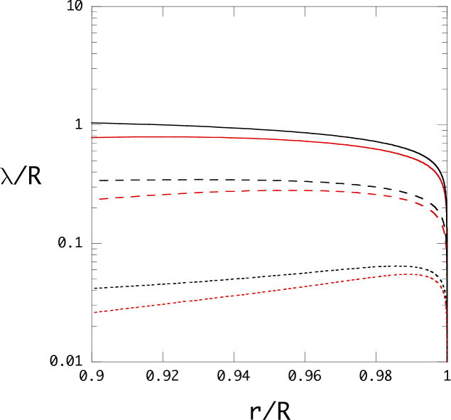
Figure 10: Local wavelengths $\lambda/R=2\pi/(Rk_{z})$ derived using the dispersion relation (21) for the $n=1$ polytrpoe of $M=1.4M_{\odot}$ and $R=10^{6}$cm and for $B_{S}=10^{15}$G, where the black lines and red lines are for $\cos\theta=0.5$ and 0, respectively, and the solid lines, dashed lines, and dotted lines are for $\cos\alpha=0.5$, 0.1, and 0.01, respectively. Here, we assume $\bar{\sigma}^{2}=10^{-5}$ (left) and $\bar{\sigma}^{2}=10^{-4}$ (right).

6 Conclusion

In this paper, we have calculated non-axisymmetric ($m\not=0$) oscillations of neutron stars magnetized with purely poloidal magnetic fields, where we have used polytropes of index $n=1$ and 1.5 as background neutron star models. We have found stable (oscillatory) magnetic modes ($\sigma^{2}>0$) of odd parity and unstable (monotonically growing) magnetic modes ($\sigma^{2}<0$) of both even and odd parity. The frequency $\sigma$ of the stable magnetic modes and the growth rate $\eta\equiv\sqrt{-\sigma^{2}}$ of the unstable magnetic modes are proportional to the magnetic field strength $B_{\rm S}=\mu_{b}/R^{3}$ measured at the surface, if the effects of buoyancy in the interior is negligible. For a given $m$, the frequency $\sigma$ and the growth rate $\eta$ decrease as the number of radial nodes of the eigenfunctions increases, which may indicate an anti-Strumian property of the problem. We have found that the non-axisymmetric magnetic modes are affected by stratification in the interior of the star, which is parametrized by using a parameter $\gamma$ in this paper. For radiative stars ($\gamma<0$), the eigenfrequency $\sigma$ of the oscillatory magnetic modes gradually increases as $|\gamma|$ increases, while it decreases with $|\gamma|$ for convective stars ($\gamma>0$). For the unstable magnetic modes, on the other hand, we have found that stable stratification with $\gamma<0$ reduces the growth rate $\eta$ of the magnetic modes, while the convectively unstable stratification enhances the growth rate as $|\gamma|$ is increased. It is also found that the growth rate $\eta$ tends to increase as the azimuthal number increases. We note that Lasky et al. (2011) obtained strong instability of magnetized star having purely poloidal magnetic field, especially for $m=4$. It has been analytically shown that purely poloidal magnetic fields having closed field lines inside the star are unstable in the limit of $m\rightarrow\infty$ (see, e.g., van Assche, Goossens, & Tayler 1982, Markey & Tayler 1973).

As mentioned in §4, we fail to obtain $f$- and $p$-modes of the magnetized star by using the present numerical code. At first glance, this fact might imply that the present numerical code and/or formulation have some problem. However, the situation at hand is not very simple, as we will discuss below. Let us assume that in the limit of $|\mbox{\boldmath$B$}|\rightarrow 0$, there exist eigensolutions for magnetized stars given by

$$\sigma=\sigma_{0}+O(\bar{\sigma}_{A}^{2})\,,\quad\mbox{\boldmath$\xi$}=\mbox{\boldmath$\xi$}_{0}+O(\bar{\sigma}_{A}^{2})\,,\quad p^{\prime}=p^{\prime}_{0}+O(\bar{\sigma}_{A}^{2})\,,\quad\rho^{\prime}=\rho^{\prime}_{0}+O(\bar{\sigma}_{A}^{2})\,,$$ (23)

where $\sigma_{0}$ is an eigenfrequency and $\mbox{\boldmath$\xi$}_{0}$, $p^{\prime}_{0}$, and $\rho^{\prime}_{0}$ are its eigenfunctions for non-magnetized stars. Clearly, Eq. (23) is an eigensolution of Eqs. (5)–(7) in conjunction with the surface boundary condition $\Delta p(r=R)=0$ in the limit of $|\mbox{\boldmath$B$}|\rightarrow 0$. From Eq. (8), we obtain

$${\mbox{\boldmath$B$}^{\prime}\over B_{S}}=\nabla\times\left(\mbox{\boldmath$\xi$}_{0}\times{\mbox{\boldmath$B$}\over B_{S}}\right)+O(\bar{\sigma}_{A}^{2})\,.$$ (24)

However, in general, this $\displaystyle{\mbox{\boldmath$B$}^{\prime}\over B_{S}}$ does not satisfy the surface boundary condition that guarantees $\displaystyle{\mbox{\boldmath$B$}^{\prime}\over B_{S}}\rightarrow 0$ as $r\rightarrow\infty$. Thus, Eqs. (23) and (24) cannot be an eigensolution for magnetized stars in the limit of $|\mbox{\boldmath$B$}|\rightarrow 0$. In other words, oscillation modes that exist in non-magnetized stars need not be present in weakly magnetized stars. From physical point of view, however, it is plausible to expect that $f$- and $p$-modes exist in magnetized stars. This apparent contradiction may be resolved if we admit that in the normal mode analysis such as we carry out in this paper the Lorentz force term in Eq. (5) must not vanish even in the limit of $|\mbox{\boldmath$B$}|\rightarrow 0$. This occurs if $\nabla\times\mbox{\boldmath$B$}^{\prime}\propto\bar{\sigma}_{A}^{-1}$ is satisfied somewhere inside the star when $|\mbox{\boldmath$B$}|\rightarrow 0$. That is to say, $\mbox{\boldmath$B$}^{\prime}$ needs to show rapid spatial oscillations somewhere inside the star to keep the Lorentz terms finite as $|\mbox{\boldmath$B$}|\rightarrow 0$. If this is the case, $f$- and $p$-modes of magnetized stars have to have slightly different eigenfrequencies and eigenfunctions form those of non-magnetized stars even in the limit of $|\mbox{\boldmath$B$}|\rightarrow 0$. In the present numerical code, it will be difficult to treat the terms related to $\nabla\times\mbox{\boldmath$B$}^{\prime}\propto\bar{\sigma}_{A}^{-1}$ accurately because we use a standard second-order accuracy finite-difference method for the radial direction and a spectral method for the $\theta$-direction, and some special technique will be required to evaluate the terms related to $\nabla\times\mbox{\boldmath$B$}^{\prime}\propto\bar{\sigma}_{A}^{-1}$ properly. Actually, we find that we can obtain ‘$f$’- and ‘$p$’-modes if we largely reduce the number of mesh points distributed in the interior for integration. This reduction in the number of mesh points may be equivalent to averaging the rapid spatial oscillations of $\mbox{\boldmath$B$}^{\prime}$ over a length scale much larger than the wavelengths of the spatial oscillations, which avoids numerical difficulty associated with rapid spatial oscillations of $\mbox{\boldmath$B$}^{\prime}$. However, we cannot consider that ‘$f$’- and ‘$p$’-modes thus obtained are correctly computed normal modes.

It is also important to note that, for given values of $m$ and $B_{S}$, we find only one magnetic mode sequence along the number of radial nodes of the eigenfunction. This result is different from that for the axisymmetric toroidal magnetic modes of stars with a poloidal field as discussed by Lee (2008) and Asai & Lee (2014), who obtained several mode sequences, differing in the surface oscillation patterns, for given $m$ and $B_{S}$. If discrete magnetic modes can exist only in the gaps between continuum frequency spectra, the difference in the distribution of continuum frequency spectra between axisymmetric $(m=0)$ toroidal modes and non-axisymmetric $(m\not=0)$ spheroidal modes, for given $m$ and $B_{S}$, might lead to the difference in the distribution of discrete magnetic modes between the two cases.

The present analysis is a part of our study of the oscillation of magnetized stars. It is well known that a purely poloidal magnetic field configuration is unstable as exemplified in this paper. Therefore, it may be difficult to observe long-lived magnetic oscillations as QPOs. However a mixed poloidal and toroidal magnetic field configuration such as twisted-torus magnetic field (e.g., Braithwaite & Spruit 2004; Yoshida & Eriguchi 2006; Yoshida, Yoshida & Eriguchi 2006; Ciolfi et al. 2009) could be stable. Thus, it is interesting to investigate stability and oscillation spectrum of the star having such a mixed magnetic field configuration. In the presence of both poloidal and toroidal field components, toroidal and spheroidal modes are coupled even for axisymmetric perturbations, which inevitably makes the analysis difficult.

As important physical properties inherent to cold neutron stars, we need to consider the effects of solid crust and those of superfluidity and super-conductivity of neutrons and protons on the oscillation modes. It is believed that neutrons become a superfluid both in the inner crust and in the fluid core while protons can be superconducting in the core. For example, if the fluid core is a type I superconductor, magnetic fields will be expelled from the core region bacause of the Meissner effect, and hence confined to the solid crust (e.g., Colaiuda et al. 2008; Sotani et al. 2008). However, a recent analysis of the spectrum of timing noise for SGR 1806-20 and SGR 1900+14 has suggested that the core region is a type II superconductor (Arras, Cumming & Thompson 2004). If this is the case, the fluid core can be threaded by a magnetic field and hence the frequency spectra of oscillation modes will be affected by the superconductivity in the core (e.g., Colaiuda et al. 2008; Sotani et al. 2008). To investigate the oscillation of magnetized stars as normal modes, taking account of the effect of superfluidity or superconductivity, will be one of our future studies (see, e.g., Glampedakis, Andersson & Samuelsson 2011; Passamonti & Lander 2013, 2014; and Gabler et al. 2013b).

Appendix A Pulsation equations for the magnetized star with purely poloidal magnetic fields

To describe the master equations concisely, it is useful to introduce the following column vectors composed of the expansion coefficients for the perturbation quantities: the vectors $S$, $H$, $T$, $\mbox{\boldmath$b$}^{S}$, $\mbox{\boldmath$b$}^{H}$, $\mbox{\boldmath$b$}^{T}$, and $\delta\mbox{\boldmath$U$}$, defined by

$$(\mbox{\boldmath$S$})_{j}=S_{l_{j}},\quad(\mbox{\boldmath$H$})_{j}=H_{l_{j}},\quad(\mbox{\boldmath$T$})_{j}=T_{l_{j}^{\prime}},\quad(\mbox{\boldmath$b$}^{S})_{j}=b^{S}_{l_{j}^{\prime}},\quad(\mbox{\boldmath$b$}^{H})_{j}=b^{H}_{l_{j}^{\prime}},\quad(\mbox{\boldmath$b$}^{T})_{j}=b^{T}_{l_{j}},\quad(\delta\mbox{\boldmath$U$})_{j}=\frac{p^{\prime}_{l_{j}}}{\rho gr},$$ (25)

where $(\mbox{\boldmath$X$})_{j}$ denotes the $j$-th component of the vector $X$ and $g=GM(r)/r^{2}$ is the gravitational acceleration. Here, $l_{j}=|m|+2(j-1)$ and $l_{j}^{\prime}=l_{j}+1$ for even modes, and $l_{j}=|m|+2j-1$ and $l_{j}^{\prime}=l_{j}-1$ for odd modes, respectively, and $j=1,2,3,...,j_{\rm max}$. The perturbed continuity equation (5) and the perturbed Euler equation (4) are then reduced to

$$r\dfrac{\mathrm{d}\mbox{\boldmath$S$}}{\mathrm{d}r}=\left(\frac{V}{\Gamma_{1}}-3\right)\mbox{\boldmath$S$}-\frac{V}{\Gamma_{1}}\delta\mbox{\boldmath$U$}+\mbox{\boldmath$\sf\Lambda$}_{0}\mbox{\boldmath$H$},$$ (26)

$$-\frac{4\pi p}{rf}Vr\dfrac{\mathrm{d}\delta\mbox{\boldmath$U$}}{\mathrm{d}r}+\frac{4\pi p}{rf}V(c_{1}\bar{\sigma}^{2}+rA)\mbox{\boldmath$S$}+\frac{4\pi p}{rf}V(1-rA-U)\delta\mbox{\boldmath$U$}$$

$$+\mbox{\boldmath$\sf C$}_{0}\left[(\mathrm{d}f+2)r\dfrac{\mathrm{d}\mbox{\boldmath$b$}^{H}}{\mathrm{d}r}-(\mathrm{d}f+2)\mbox{\boldmath$b$}^{S}+(\mathrm{d}^{2}f+6\mathrm{d}f+4)\mbox{\boldmath$b$}^{H}\right]+m\left[(\mathrm{d}f+2)r\dfrac{\mathrm{d}\mbox{\boldmath$b$}^{T}}{\mathrm{d}r}+(\mathrm{d}^{2}f+6\mathrm{d}f+4)\mbox{\boldmath$b$}^{T}\right]=0,$$ (27)

$$\frac{V}{\Gamma_{1}}\delta\mbox{\boldmath$U$}=\frac{V}{\Gamma_{1}}c_{1}\bar{\sigma}^{2}(\mathrm{d}f+2)\mbox{\boldmath$\sf A$}_{1}^{-1}\mbox{\boldmath$\sf B$}_{1}\mbox{\boldmath$S$}-\frac{V}{\Gamma_{1}}mc_{1}\bar{\sigma}^{2}(\mbox{\boldmath$\sf A$}_{1}^{-1}+\mbox{\boldmath$\sf\Lambda$}_{0}^{-1}\mbox{\boldmath$\sf A$}_{1}^{-1}\mbox{\boldmath$\sf\Lambda$}_{1})\mbox{\boldmath$T$}+\bigg{\{}\frac{V}{\Gamma_{1}}c_{1}\bar{\sigma}^{2}\frac{r}{2f}\mbox{\boldmath$\sf A$}_{1}^{-1}$$

$$+\frac{rf}{2\pi\Gamma_{1}p}\left[(\mathrm{d}^{2}f+4\mathrm{d}f)\mbox{\boldmath$\sf\Lambda$}_{0}^{-1}\mbox{\boldmath$\sf B$}_{0}-\mbox{\boldmath$\sf\Lambda$}_{0}^{-1}\mbox{\boldmath$\sf A$}_{0}+\frac{1}{2}m^{2}(\mathrm{d}^{2}f+4\mathrm{d}f+2)\mbox{\boldmath$\sf\Lambda$}_{0}^{-1}\mbox{\boldmath$\sf A$}_{1}^{-1}\right]\bigg{\}}\mbox{\boldmath$b$}^{S}$$

$$+\frac{rf}{\pi\Gamma_{1}p}(\mbox{\boldmath$\sf\Lambda$}_{0}^{-1}\mbox{\boldmath$\sf A$}_{0}-m^{2}\mbox{\boldmath$\sf\Lambda$}_{0}^{-1}\mbox{\boldmath$\sf A$}_{1}^{-1})\mbox{\boldmath$b$}^{H}+\frac{rf}{2\pi\Gamma_{1}p}m\bigg{[}\frac{1}{2}(\mathrm{d}f+2)\mbox{\boldmath$\sf I$}+2\mbox{\boldmath$\sf\Lambda$}_{0}^{-1}$$

$$\mathrm{d}f\mbox{\boldmath$\sf\Lambda$}_{0}^{-1}\mbox{\boldmath$\sf A$}_{1}^{-1}\mbox{\boldmath$\sf B$}_{1}\mbox{\boldmath$\sf\Lambda$}_{0}+\mbox{\boldmath$\sf\Lambda$}_{0}^{-1}\mbox{\boldmath$\sf A$}_{1}^{-1}\tilde{\mbox{\boldmath$\sf C$}}_{1}\bigg{]}\mbox{\boldmath$b$}^{T}+\frac{rf}{2\pi\Gamma_{1}p}\mbox{\boldmath$\sf\Lambda$}_{0}^{-1}\mbox{\boldmath$\sf A$}_{0}\mbox{\boldmath$\sf L$}_{0}r\dfrac{\mathrm{d}\mbox{\boldmath$b$}^{H}}{\mathrm{d}r},$$ (28)

$$\mbox{\boldmath$\sf A$}_{1}r\dfrac{\mathrm{d}\mbox{\boldmath$b$}^{T}}{\mathrm{d}r}=-\frac{2\pi p}{rf}Vc_{1}\bar{\sigma}^{2}\mbox{\boldmath$\sf\Lambda$}_{1}\mbox{\boldmath$T$}+\frac{1}{2}m(\mathrm{d}^{2}f+4\mathrm{d}f+2)\mbox{\boldmath$b$}^{S}-2m\mbox{\boldmath$b$}^{H}+\left(\mathrm{d}f\mbox{\boldmath$\sf B$}_{1}\mbox{\boldmath$\sf\Lambda$}_{0}+\tilde{\mbox{\boldmath$\sf C$}}_{1}\right)\mbox{\boldmath$b$}^{T}-mr\dfrac{\mathrm{d}\mbox{\boldmath$b$}^{H}}{\mathrm{d}r}.$$ (29)

Substituting $\delta\mbox{\boldmath$U$}$ given in (A4) into (A3), we may obtain

$$\mbox{\boldmath$\sf L$}_{0}r\dfrac{\mathrm{d}}{\mathrm{d}r}\left(r\dfrac{\mathrm{d}\mbox{\boldmath$b$}^{H}}{\mathrm{d}r}\right)=\frac{2\pi p}{rf}V\left(c_{1}\bar{\sigma}^{2}+rA\right)\mbox{\boldmath$\sf A$}_{0}^{-1}\mbox{\boldmath$\sf\Lambda$}_{0}\mbox{\boldmath$S$}+\frac{4\pi p}{rf}mVc_{1}\bar{\sigma}^{2}\mbox{\boldmath$\sf A$}_{0}^{-1}\mbox{\boldmath$\sf A$}_{1}^{-1}\mbox{\boldmath$\sf\Lambda$}_{1}\mbox{\boldmath$T$}+\bigg{\{}-\frac{1}{2}\left(\mathrm{d}f+2\right)\mbox{\boldmath$\sf A$}_{0}^{-1}\tilde{\mbox{\boldmath$\sf C$}}_{0}-\left(\mathrm{d}\rho-rA+4\right)\mbox{\boldmath$\sf I$}$$

$$+\left[-\mathrm{d}^{3}f+\mathrm{d}^{2}f\left(\mathrm{d}\rho-rA-4\right)+4\mathrm{d}f\left(\mathrm{d}\rho-rA+1\right)\right]\mbox{\boldmath$\sf A$}_{0}^{-1}\mbox{\boldmath$\sf B$}_{0}-\frac{1}{2}\big{[}\mathrm{d}^{3}f-\mathrm{d}^{2}f(\mathrm{d}\rho-4)$$

$$-2\mathrm{d}f(2\mathrm{d}\rho+1)-2(\mathrm{d}\rho+2)\big{]}m^{2}\mbox{\boldmath$\sf A$}_{0}^{-1}\mbox{\boldmath$\sf A$}_{1}^{-1}\bigg{\}}\mbox{\boldmath$b$}^{S}+\bigg{[}(\mathrm{d}f+1)\mbox{\boldmath$\sf A$}_{0}^{-1}\tilde{\mbox{\boldmath$\sf C$}}_{0}+\mbox{\boldmath$\sf\Lambda$}_{1}+2\mbox{\boldmath$\sf A$}_{0}^{-1}\mbox{\boldmath$\sf B$}_{0}\mbox{\boldmath$\sf\Lambda$}_{1}+2(\mathrm{d}\rho-rA)\mbox{\boldmath$\sf I$}$$

$$-\frac{1}{2}(\mathrm{d}^{2}f+4\mathrm{d}f+2)m^{2}\mbox{\boldmath$\sf A$}_{0}^{-1}\mbox{\boldmath$\sf A$}_{1}^{-1}\tilde{\mbox{\boldmath$\sf\Lambda$}}_{1}-(\mathrm{d}^{2}f+2\mathrm{d}f+2\mathrm{d}\rho)m^{2}\mbox{\boldmath$\sf A$}_{0}^{-1}\mbox{\boldmath$\sf A$}_{1}^{-1}\bigg{]}\mbox{\boldmath$b$}^{H}$$

$$+\Bigg{\{}-m\bigg{\{}2(\mathrm{d}f-\mathrm{d}\rho+rA+1)\mbox{\boldmath$\sf A$}_{0}^{-1}+\frac{1}{2}[-\mathrm{d}f(\mathrm{d}\rho+2)+(\mathrm{d}f+2)rA-2(\mathrm{d}\rho+1)]\mbox{\boldmath$\sf A$}_{0}^{-1}\mbox{\boldmath$\sf\Lambda$}_{0}\bigg{\}}$$

$$-m\left[(\mathrm{d}^{2}f-\mathrm{d}\rho\mathrm{d}f+2\mathrm{d}f)\mbox{\boldmath$\sf A$}_{0}^{-1}\mbox{\boldmath$\sf A$}_{1}^{-1}\mbox{\boldmath$\sf B$}_{1}\mbox{\boldmath$\sf\Lambda$}_{0}+(\mathrm{d}f-\mathrm{d}\rho+1)\mbox{\boldmath$\sf A$}_{0}^{-1}\mbox{\boldmath$\sf A$}_{1}^{-1}\tilde{\mbox{\boldmath$\sf C$}}_{1}\right]\Bigg{\}}\mbox{\boldmath$b$}^{T}$$

$$+\left[\frac{1}{2}(\mathrm{d}f+2)\mbox{\boldmath$\sf A$}_{0}^{-1}\tilde{\mbox{\boldmath$\sf C$}}_{0}+(\mathrm{d}\rho-rA-1)\mbox{\boldmath$\sf I$}+m^{2}(\mathrm{d}f-\mathrm{d}\rho+3)\mbox{\boldmath$\sf A$}_{0}^{-1}\mbox{\boldmath$\sf A$}_{1}^{-1}\right]r\dfrac{\mathrm{d}\mbox{\boldmath$b$}^{H}}{\mathrm{d}r}-\frac{2\pi p}{rf}(2+rA)Vc_{1}\bar{\sigma}^{2}\mbox{\boldmath$\sf A$}_{0}^{-1}\mbox{\boldmath$\sf\Lambda$}_{0}\mbox{\boldmath$H$}$$

$$-\frac{2\pi p}{rf}Vc_{1}\bar{\sigma}^{2}\mbox{\boldmath$\sf A$}_{0}^{-1}\mbox{\boldmath$\sf\Lambda$}_{0}r\dfrac{\mathrm{d}\mbox{\boldmath$H$}}{\mathrm{d}r}+\frac{2\pi p}{rf}mVc_{1}\bar{\sigma}^{2}\mbox{\boldmath$\sf A$}_{0}^{-1}\mbox{\boldmath$\sf A$}_{1}^{-1}\mbox{\boldmath$\sf\Lambda$}_{1}r\dfrac{\mathrm{d}\mbox{\boldmath$T$}}{\mathrm{d}r}-m\left[\frac{1}{2}(\mathrm{d}f+2)\mbox{\boldmath$\sf A$}_{0}^{-1}\mbox{\boldmath$\sf A$}_{1}^{-1}\tilde{\mbox{\boldmath$\sf C$}}_{1}+(\mathrm{d}f+rA+2)\mbox{\boldmath$\sf A$}_{0}^{-1}\right]r\dfrac{\mathrm{d}\mbox{\boldmath$b$}^{T}}{\mathrm{d}r}.$$ (30)

The perturbed induction equation (7) and the perturbed Gauss’s law for magnetic fields are reduced to

$$\mbox{\boldmath$H$}=(\mathrm{d}f+2)\mbox{\boldmath$\sf A$}_{1}^{-1}\mbox{\boldmath$\sf B$}_{1}\mbox{\boldmath$S$}-m\mbox{\boldmath$\sf A$}_{1}^{-1}\mbox{\boldmath$T$}+\frac{r}{2f}\mbox{\boldmath$\sf A$}_{1}^{-1}\mbox{\boldmath$b$}^{S},$$ (31)

$$\mbox{\boldmath$\sf L$}_{0}r\dfrac{\mathrm{d}\mbox{\boldmath$T$}}{\mathrm{d}r}=-m\left[\mathrm{d}^{2}f+\left(2+\frac{V}{\Gamma_{1}}\right)\mathrm{d}f-2\left(1-\frac{V}{\Gamma_{1}}\right)\right]\left(\mbox{\boldmath$\sf A$}_{0}^{-1}\mbox{\boldmath$\sf A$}_{1}^{-1}\mbox{\boldmath$\sf B$}_{1}+\frac{1}{2}\mbox{\boldmath$\sf A$}_{0}^{-1}\right)\mbox{\boldmath$S$}+\left(\mathrm{d}f+2\right)\left(m^{2}\mbox{\boldmath$\sf A$}_{0}^{-1}\mbox{\boldmath$\sf A$}_{1}^{-1}+\frac{1}{2}\mbox{\boldmath$\sf A$}_{0}^{-1}\tilde{\mbox{\boldmath$\sf C$}}_{0}\right)\mbox{\boldmath$T$}$$

$$-\frac{r}{2f}m\mbox{\boldmath$\sf A$}_{0}^{-1}\mbox{\boldmath$\sf A$}_{1}^{-1}\mbox{\boldmath$\sf\Lambda$}_{1}\mbox{\boldmath$b$}^{H}+\frac{r}{2f}\mbox{\boldmath$\sf A$}_{0}^{-1}\mbox{\boldmath$\sf\Lambda$}_{0}\mbox{\boldmath$b$}^{T}-m\left(\mathrm{d}f+2\right)\left(\mbox{\boldmath$\sf A$}_{0}^{-1}+\frac{1}{2}\mbox{\boldmath$\sf A$}_{0}^{-1}\mbox{\boldmath$\sf A$}_{1}^{-1}\tilde{\mbox{\boldmath$\sf C$}}_{1}\right)\mbox{\boldmath$H$}$$

$$+m\left(\mathrm{d}f+2\right)\left(\mbox{\boldmath$\sf A$}_{0}^{-1}\mbox{\boldmath$\sf A$}_{1}^{-1}\mbox{\boldmath$\sf B$}_{1}+\frac{1}{2}\mbox{\boldmath$\sf A$}_{0}^{-1}\right)\frac{V}{\Gamma_{1}}\delta\mbox{\boldmath$U$},$$ (32)

$$\mbox{\boldmath$\sf L$}_{1}r\dfrac{\mathrm{d}\mbox{\boldmath$H$}}{\mathrm{d}r}=\left[\mathrm{d}^{2}f+\left(2+\frac{V}{\Gamma_{1}}\right)\mathrm{d}f-2\left(1-\frac{V}{\Gamma_{1}}\right)\right]\left(\mbox{\boldmath$\sf A$}_{1}^{-1}\mbox{\boldmath$\sf B$}_{1}+\frac{1}{2}m^{2}\mbox{\boldmath$\sf A$}_{1}^{-1}\mbox{\boldmath$\sf A$}_{0}^{-1}\right)\mbox{\boldmath$S$}-m\left(\mathrm{d}f+2\right)\left(\mbox{\boldmath$\sf A$}_{1}^{-1}+\frac{1}{2}\mbox{\boldmath$\sf A$}_{1}^{-1}\mbox{\boldmath$\sf A$}_{0}^{-1}\tilde{\mbox{\boldmath$\sf C$}}_{0}\right)\mbox{\boldmath$T$}$$

$$+\frac{r}{2f}\mbox{\boldmath$\sf A$}_{1}^{-1}\mbox{\boldmath$\sf\Lambda$}_{1}\mbox{\boldmath$b$}^{H}-\frac{r}{2f}m\mbox{\boldmath$\sf A$}_{1}^{-1}\mbox{\boldmath$\sf A$}_{0}^{-1}\mbox{\boldmath$\sf\Lambda$}_{0}\mbox{\boldmath$b$}^{T}+\left(\mathrm{d}f+2\right)\left(m^{2}\mbox{\boldmath$\sf A$}_{1}^{-1}\mbox{\boldmath$\sf A$}_{0}^{-1}+\frac{1}{2}\mbox{\boldmath$\sf A$}_{1}^{-1}\tilde{\mbox{\boldmath$\sf C$}}_{1}\right)\mbox{\boldmath$H$}$$

$$-\left(\mathrm{d}f+2\right)\left(\mbox{\boldmath$\sf A$}_{1}^{-1}\mbox{\boldmath$\sf B$}_{1}+\frac{1}{2}m^{2}\mbox{\boldmath$\sf A$}_{1}^{-1}\mbox{\boldmath$\sf A$}_{0}^{-1}\right)\frac{V}{\Gamma_{1}}\delta\mbox{\boldmath$U$},$$ (33)

$$r\dfrac{\mathrm{d}\mbox{\boldmath$b$}^{S}}{\mathrm{d}r}=-3\mbox{\boldmath$b$}^{S}+\mbox{\boldmath$\sf\Lambda$}_{1}\mbox{\boldmath$b$}^{H}.$$ (34)

Here

$$V=-\dfrac{\mathrm{d}\ln p}{\mathrm{d}\ln r},\quad c_{1}=\frac{M}{M(r)}\left(\frac{r}{R}\right)^{3},\quad\mathrm{d}\rho=\dfrac{\mathrm{d}\ln\rho}{\mathrm{d}\ln r},\quad\mathrm{d}f=\dfrac{\mathrm{d}\ln f}{\mathrm{d}\ln r},\quad\mathrm{d}^{2}f=\frac{r^{2}}{f}\dfrac{\mathrm{d}^{2}f}{\mathrm{d}r^{2}},\quad\mathrm{d}^{3}f=\frac{r^{3}}{f}\dfrac{\mathrm{d}^{3}f}{\mathrm{d}r^{3}},$$ (35)

and $\bar{\sigma}\equiv\sigma/(GM/R^{3})^{1/2}$ is the frequency in the unit of the Kepler frequency of the star. The quantities $\mbox{\boldmath$\sf A$}_{0}$, $\mbox{\boldmath$\sf A$}_{1}$, $\mbox{\boldmath$\sf B$}_{0}$, $\mbox{\boldmath$\sf B$}_{1}$, $\tilde{\mbox{\boldmath$\sf C$}}_{0}$, $\tilde{\mbox{\boldmath$\sf C$}}_{1}$, $\tilde{\mbox{\boldmath$\sf\Lambda$}}_{0}$, $\tilde{\mbox{\boldmath$\sf\Lambda$}}_{1}$, $\mbox{\boldmath$\sf L$}_{0}$, and $\mbox{\boldmath$\sf L$}_{1}$ denote the matrices defined as follows:

$$\mbox{\boldmath$\sf A$}_{0}=\mbox{\boldmath$\sf C$}_{0}+\mbox{\boldmath$\sf Q$}_{0}\mbox{\boldmath$\sf\Lambda$}_{1},\quad\mbox{\boldmath$\sf A$}_{1}=\mbox{\boldmath$\sf C$}_{1}+\mbox{\boldmath$\sf Q$}_{1}\mbox{\boldmath$\sf\Lambda$}_{0},\quad\mbox{\boldmath$\sf B$}_{0}=\mbox{\boldmath$\sf Q$}_{0}+\frac{1}{2}\mbox{\boldmath$\sf C$}_{0},\quad\mbox{\boldmath$\sf B$}_{1}=\mbox{\boldmath$\sf Q$}_{1}+\frac{1}{2}\mbox{\boldmath$\sf C$}_{1},$$

$$\tilde{\mbox{\boldmath$\sf C$}}_{0}=\mbox{\boldmath$\sf C$}_{0}(\mbox{\boldmath$\sf\Lambda$}_{1}-2\mbox{\boldmath$\sf I$}),\quad\tilde{\mbox{\boldmath$\sf C$}}_{1}=\mbox{\boldmath$\sf C$}_{1}(\mbox{\boldmath$\sf\Lambda$}_{0}-2\mbox{\boldmath$\sf I$}),\quad\tilde{\mbox{\boldmath$\sf\Lambda$}}_{0}=\mbox{\boldmath$\sf\Lambda$}_{0}-2\mbox{\boldmath$\sf I$},\quad\tilde{\mbox{\boldmath$\sf\Lambda$}}_{1}=\mbox{\boldmath$\sf\Lambda$}_{1}-2\mbox{\boldmath$\sf I$},$$

$$\mbox{\boldmath$\sf L$}_{0}=\mbox{\boldmath$\sf I$}-m^{2}\mbox{\boldmath$\sf A$}_{0}^{-1}\mbox{\boldmath$\sf A$}_{1}^{-1},\quad\mbox{\boldmath$\sf L$}_{1}=\mbox{\boldmath$\sf I$}-m^{2}\mbox{\boldmath$\sf A$}_{1}^{-1}\mbox{\boldmath$\sf A$}_{0}^{-1}.$$ (36)

The matrices $\mbox{\boldmath$\sf Q$}_{0}$, $\mbox{\boldmath$\sf Q$}_{1}$, $\mbox{\boldmath$\sf C$}_{0}$, $\mbox{\boldmath$\sf C$}_{1}$, $\mbox{\boldmath$\sf\Lambda$}_{0}$, and $\mbox{\boldmath$\sf\Lambda$}_{1}$ are defined as follows:

For even modes,

$$(\mbox{\boldmath$\sf Q$}_{0})_{jj}=J_{l_{j}+1}^{m},\quad(\mbox{\boldmath$\sf Q$}_{0})_{j+1,j}=J_{l_{j}+2}^{m},\quad(\mbox{\boldmath$\sf Q$}_{1})_{jj}=J_{l_{j}+1}^{m},\quad(\mbox{\boldmath$\sf Q$}_{1})_{j,j+1}=J_{l_{j}+2}^{m},$$

$$(\mbox{\boldmath$\sf C$}_{0})_{jj}=-(l_{j}+2)J_{l_{j}+1}^{m},\quad(\mbox{\boldmath$\sf C$}_{0})_{j+1,j}=(l_{j}+1)J_{l_{j}+2}^{m},\quad(\mbox{\boldmath$\sf C$}_{1})_{jj}=l_{j}J_{l_{j}+1}^{m},\quad(\mbox{\boldmath$\sf C$}_{1})_{j,j+1}=-(l_{j}+3)J_{l_{j}+2}^{m},$$

$$(\mbox{\boldmath$\sf\Lambda$}_{0})_{jj}=l_{j}(l_{j}+1),\quad(\mbox{\boldmath$\sf\Lambda$}_{1})_{jj}=(l_{j}+1)(l_{j}+2),$$ (37)

where $l_{j}=|m|+2j-2$ for $j=1,2,3,....,j_{\rm max}$, and

$$J_{l_{j}}^{m}=\left[\frac{(l_{j}+m)(l_{j}-m)}{(2l_{j}-1)(2l_{j}+1)}\right]^{1/2}.$$ (38)

For odd modes,

$$(\mbox{\boldmath$\sf Q$}_{0})_{jj}=J_{l_{j}+1}^{m},\quad(\mbox{\boldmath$\sf Q$}_{0})_{j,j+1}=J_{l_{j}+2}^{m},\quad(\mbox{\boldmath$\sf Q$}_{1})_{jj}=J_{l_{j}+1}^{m},\quad(\mbox{\boldmath$\sf Q$}_{1})_{j+1,j}=J_{l_{j}+2}^{m},$$

$$(\mbox{\boldmath$\sf C$}_{0})_{jj}=l_{j}J_{l_{j}+1}^{m},\quad(\mbox{\boldmath$\sf C$}_{0})_{j,j+1}=-(l_{j}+3)J_{l_{j}+2}^{m},\quad(\mbox{\boldmath$\sf C$}_{1})_{jj}=-(l_{j}+2)J_{l_{j}+1}^{m},\quad(\mbox{\boldmath$\sf C$}_{1})_{j+1,j}=(l_{j}+1)J_{l_{j}+2}^{m},$$

$$(\mbox{\boldmath$\sf\Lambda$}_{0})_{jj}=(l_{j}+1)(l_{j}+2),\quad(\mbox{\boldmath$\sf\Lambda$}_{1})_{jj}=l_{j}(l_{j}+1),$$ (39)

where $l_{j}=|m|+2j-1$ for $j=1,2,3,....,j_{\rm max}$.

From the equations given before, we see that non-axisymmetric pulsations of the magnetized star with purely poloidal magnetic fields may be described by a system of $6j_{\rm max}$-th order ordinary differential equations. In this study, we chose the column vectors $S$, $T$, $\mbox{\boldmath$b$}^{S}$, $\mbox{\boldmath$b$}^{H}$, $\mbox{\boldmath$b$}^{T}$, and $\displaystyle r{\mathrm{d}\over\mathrm{d}r}\mbox{\boldmath$b$}^{H}$ as dependent variables. If the dimensionless vector variables, defined by

$$\mbox{\boldmath$y$}_{1}=\mbox{\boldmath$S$},\quad\mbox{\boldmath$y$}_{2}=\mbox{\boldmath$T$},\quad\mbox{\boldmath$y$}_{3}=\mbox{\boldmath$h$}^{S},\quad\mbox{\boldmath$y$}_{4}=\mbox{\boldmath$h$}^{H},\quad\mbox{\boldmath$y$}_{5}=\mbox{\boldmath$h$}^{T},\quad\mbox{\boldmath$y$}_{6}=r\dfrac{\mathrm{d}}{\mathrm{d}r}\mbox{\boldmath$h$}^{H},$$ (40)

where $\mbox{\boldmath$h$}^{i}\equiv[R/f(0)]\mbox{\boldmath$b$}^{i}$ for $i=S,H,T$, are introduced, the master equations for stellar pulsations are schematically written by the coupled first-order differential equations, given by

$$r\dfrac{\mathrm{d}\mbox{\boldmath$y$}_{1}}{\mathrm{d}r}=\mbox{\boldmath$\sf{\cal{F}}$}_{11}\mbox{\boldmath$y$}_{1}+\mbox{\boldmath$\sf\Lambda$}_{0}\mbox{\boldmath$H$}-\frac{V}{\Gamma_{1}}\delta\mbox{\boldmath$U$}\ \ \ \ \ \ \ \ \ \ \ \ \ \ \ \ \ \ \ \ \ \ \ \ \ \ \ \ \ \ \ \ \ \ \ \ \ \ \ \ \ \ \ \ \ \ \ \ \ \ \ \ \ \ \ \ \ \ \ \ \ \ \ \ \ \ \ \ \ \ \ \ \ \ \ \ \ \ \ \ \ \ \ \ \ \ \ \ \$$

$$\ \ \ \ \ \ \ =(\mbox{\boldmath$\sf{\cal{F}}$}_{11}-\mbox{\boldmath$\sf{\cal{E}}$}_{11}+\mbox{\boldmath$\sf\Lambda$}_{0}\mbox{\boldmath$\sf{\cal{E}}$}_{21})\mbox{\boldmath$y$}_{1}+(-\mbox{\boldmath$\sf{\cal{E}}$}_{12}+\mbox{\boldmath$\sf\Lambda$}_{0}\mbox{\boldmath$\sf{\cal{E}}$}_{22})\mbox{\boldmath$y$}_{2}+(-\mbox{\boldmath$\sf{\cal{E}}$}_{13}+\mbox{\boldmath$\sf\Lambda$}_{0}\mbox{\boldmath$\sf{\cal{E}}$}_{23})\mbox{\boldmath$y$}_{3}-\mbox{\boldmath$\sf{\cal{E}}$}_{14}\mbox{\boldmath$y$}_{4}-\mbox{\boldmath$\sf{\cal{E}}$}_{15}\mbox{\boldmath$y$}_{5}-\mbox{\boldmath$\sf{\cal{E}}$}_{16}\mbox{\boldmath$y$}_{6},$$ (41)

$$r\dfrac{\mathrm{d}\mbox{\boldmath$y$}_{2}}{\mathrm{d}r}=\mbox{\boldmath$\sf{\cal{F}}$}_{21}\mbox{\boldmath$y$}_{1}+\mbox{\boldmath$\sf{\cal{F}}$}_{22}\mbox{\boldmath$y$}_{2}+\mbox{\boldmath$\sf{\cal{F}}$}_{24}\mbox{\boldmath$y$}_{4}+\mbox{\boldmath$\sf{\cal{F}}$}_{25}\mbox{\boldmath$y$}_{5}+\mbox{\boldmath$\sf{\cal{G}}$}_{21}\frac{V}{\Gamma_{1}}\delta\mbox{\boldmath$U$}+\mbox{\boldmath$\sf{\cal{G}}$}_{22}\mbox{\boldmath$H$}\ \ \ \ \ \ \ \ \ \ \ \ \ \ \ \ \ \ \ \ \ \ \ \ \ \ \ \ \ \ \ \ \ \$$

$$\ \ \ \ \ \ =(\mbox{\boldmath$\sf{\cal{F}}$}_{21}+\mbox{\boldmath$\sf{\cal{G}}$}_{21}\mbox{\boldmath$\sf{\cal{E}}$}_{11}+\mbox{\boldmath$\sf{\cal{G}}$}_{22}\mbox{\boldmath$\sf{\cal{E}}$}_{21})\mbox{\boldmath$y$}_{1}+(\mbox{\boldmath$\sf{\cal{F}}$}_{22}+\mbox{\boldmath$\sf{\cal{G}}$}_{21}\mbox{\boldmath$\sf{\cal{E}}$}_{12}+\mbox{\boldmath$\sf{\cal{G}}$}_{22}\mbox{\boldmath$\sf{\cal{E}}$}_{22})\mbox{\boldmath$y$}_{2}+(\mbox{\boldmath$\sf{\cal{G}}$}_{21}\mbox{\boldmath$\sf{\cal{E}}$}_{13}+\mbox{\boldmath$\sf{\cal{G}}$}_{22}\mbox{\boldmath$\sf{\cal{E}}$}_{23})\mbox{\boldmath$y$}_{3}$$

$$+(\mbox{\boldmath$\sf{\cal{F}}$}_{24}+\mbox{\boldmath$\sf{\cal{G}}$}_{21}\mbox{\boldmath$\sf{\cal{E}}$}_{14})\mbox{\boldmath$y$}_{4}+(\mbox{\boldmath$\sf{\cal{F}}$}_{25}+\mbox{\boldmath$\sf{\cal{G}}$}_{21}\mbox{\boldmath$\sf{\cal{E}}$}_{15})\mbox{\boldmath$y$}_{5}+\mbox{\boldmath$\sf{\cal{G}}$}_{21}\mbox{\boldmath$\sf{\cal{E}}$}_{16}\mbox{\boldmath$y$}_{6},$$ (42)

$$r\dfrac{\mathrm{d}\mbox{\boldmath$y$}_{3}}{\mathrm{d}r}=-3\mbox{\boldmath$y$}_{3}+\mbox{\boldmath$\sf\Lambda$}_{1}\mbox{\boldmath$y$}_{4},$$ (43)

$$r\dfrac{\mathrm{d}\mbox{\boldmath$y$}_{4}}{\mathrm{d}r}=\mbox{\boldmath$y$}_{6},$$ (44)

$$r\dfrac{\mathrm{d}\mbox{\boldmath$y$}_{5}}{\mathrm{d}r}=\mbox{\boldmath$\sf{\cal{F}}$}_{52}\mbox{\boldmath$y$}_{2}+\mbox{\boldmath$\sf{\cal{F}}$}_{53}\mbox{\boldmath$y$}_{3}+\mbox{\boldmath$\sf{\cal{F}}$}_{54}\mbox{\boldmath$y$}_{4}+\mbox{\boldmath$\sf{\cal{F}}$}_{55}\mbox{\boldmath$y$}_{5}+\mbox{\boldmath$\sf{\cal{F}}$}_{56}\mbox{\boldmath$y$}_{6},$$ (45)

$$r\dfrac{\mathrm{d}\mbox{\boldmath$y$}_{6}}{\mathrm{d}r}=\mbox{\boldmath$\sf{\cal{F}}$}_{61}\mbox{\boldmath$y$}_{1}+\mbox{\boldmath$\sf{\cal{F}}$}_{62}\mbox{\boldmath$y$}_{2}+\mbox{\boldmath$\sf{\cal{F}}$}_{63}\mbox{\boldmath$y$}_{3}+\mbox{\boldmath$\sf{\cal{F}}$}_{64}\mbox{\boldmath$y$}_{4}+\mbox{\boldmath$\sf{\cal{F}}$}_{65}\mbox{\boldmath$y$}_{5}+\mbox{\boldmath$\sf{\cal{F}}$}_{66}\mbox{\boldmath$y$}_{6}+\mbox{\boldmath$\sf{\cal{G}}$}_{62}\mbox{\boldmath$H$}+\mbox{\boldmath$\sf{\cal{G}}$}_{63}r\dfrac{\mathrm{d}\mbox{\boldmath$H$}}{\mathrm{d}r}+\mbox{\boldmath$\sf{\cal{G}}$}_{64}r\dfrac{\mathrm{d}\mbox{\boldmath$y$}_{2}}{\mathrm{d}r}+\mbox{\boldmath$\sf{\cal{G}}$}_{65}r\dfrac{\mathrm{d}\mbox{\boldmath$y$}_{5}}{\mathrm{d}r}$$

$$=\left[\mbox{\boldmath$\sf{\cal{F}}$}_{61}+\mbox{\boldmath$\sf{\cal{G}}$}_{62}\mbox{\boldmath$\sf{\cal{E}}$}_{21}+\mbox{\boldmath$\sf{\cal{G}}$}_{63}(\mbox{\boldmath$\sf{\cal{E}}$}_{31}+\mbox{\boldmath$\sf{\cal{E}}$}_{37}\mbox{\boldmath$\sf{\cal{E}}$}_{21}+\mbox{\boldmath$\sf{\cal{E}}$}_{38}\mbox{\boldmath$\sf{\cal{E}}$}_{11})+\mbox{\boldmath$\sf{\cal{G}}$}_{64}(\mbox{\boldmath$\sf{\cal{F}}$}_{21}+\mbox{\boldmath$\sf{\cal{G}}$}_{21}\mbox{\boldmath$\sf{\cal{E}}$}_{11}+\mbox{\boldmath$\sf{\cal{G}}$}_{22}\mbox{\boldmath$\sf{\cal{E}}$}_{21})\right]\mbox{\boldmath$y$}_{1}$$

$$+\left[\mbox{\boldmath$\sf{\cal{F}}$}_{62}+\mbox{\boldmath$\sf{\cal{G}}$}_{62}\mbox{\boldmath$\sf{\cal{E}}$}_{22}+\mbox{\boldmath$\sf{\cal{G}}$}_{63}(\mbox{\boldmath$\sf{\cal{E}}$}_{32}+\mbox{\boldmath$\sf{\cal{E}}$}_{37}\mbox{\boldmath$\sf{\cal{E}}$}_{22}+\mbox{\boldmath$\sf{\cal{E}}$}_{38}\mbox{\boldmath$\sf{\cal{E}}$}_{12})+\mbox{\boldmath$\sf{\cal{G}}$}_{64}(\mbox{\boldmath$\sf{\cal{F}}$}_{22}+\mbox{\boldmath$\sf{\cal{G}}$}_{21}\mbox{\boldmath$\sf{\cal{E}}$}_{12}+\mbox{\boldmath$\sf{\cal{G}}$}_{22}\mbox{\boldmath$\sf{\cal{E}}$}_{22})+\mbox{\boldmath$\sf{\cal{G}}$}_{65}\mbox{\boldmath$\sf{\cal{F}}$}_{52}\right]\mbox{\boldmath$y$}_{2}$$

$$+\left[\mbox{\boldmath$\sf{\cal{F}}$}_{63}+\mbox{\boldmath$\sf{\cal{G}}$}_{62}\mbox{\boldmath$\sf{\cal{E}}$}_{23}+\mbox{\boldmath$\sf{\cal{G}}$}_{63}(\mbox{\boldmath$\sf{\cal{E}}$}_{37}\mbox{\boldmath$\sf{\cal{E}}$}_{23}+\mbox{\boldmath$\sf{\cal{E}}$}_{38}\mbox{\boldmath$\sf{\cal{E}}$}_{13})+\mbox{\boldmath$\sf{\cal{G}}$}_{64}(\mbox{\boldmath$\sf{\cal{G}}$}_{21}\mbox{\boldmath$\sf{\cal{E}}$}_{13}+\mbox{\boldmath$\sf{\cal{G}}$}_{22}\mbox{\boldmath$\sf{\cal{E}}$}_{23})+\mbox{\boldmath$\sf{\cal{G}}$}_{65}\mbox{\boldmath$\sf{\cal{F}}$}_{53}\right]\mbox{\boldmath$y$}_{3}$$

$$+\left[\mbox{\boldmath$\sf{\cal{F}}$}_{64}+\mbox{\boldmath$\sf{\cal{G}}$}_{63}(\mbox{\boldmath$\sf{\cal{E}}$}_{34}+\mbox{\boldmath$\sf{\cal{E}}$}_{38}\mbox{\boldmath$\sf{\cal{E}}$}_{14})+\mbox{\boldmath$\sf{\cal{G}}$}_{64}(\mbox{\boldmath$\sf{\cal{F}}$}_{24}+\mbox{\boldmath$\sf{\cal{G}}$}_{21}\mbox{\boldmath$\sf{\cal{E}}$}_{14})+\mbox{\boldmath$\sf{\cal{G}}$}_{65}\mbox{\boldmath$\sf{\cal{F}}$}_{54}\right]\mbox{\boldmath$y$}_{4}$$

$$+\left[\mbox{\boldmath$\sf{\cal{F}}$}_{65}+\mbox{\boldmath$\sf{\cal{G}}$}_{63}(\mbox{\boldmath$\sf{\cal{E}}$}_{35}+\mbox{\boldmath$\sf{\cal{E}}$}_{38}\mbox{\boldmath$\sf{\cal{E}}$}_{15})+\mbox{\boldmath$\sf{\cal{G}}$}_{64}(\mbox{\boldmath$\sf{\cal{F}}$}_{25}+\mbox{\boldmath$\sf{\cal{G}}$}_{21}\mbox{\boldmath$\sf{\cal{E}}$}_{15})+\mbox{\boldmath$\sf{\cal{G}}$}_{65}\mbox{\boldmath$\sf{\cal{F}}$}_{55}\right]\mbox{\boldmath$y$}_{5}$$

$$+\left(\mbox{\boldmath$\sf{\cal{F}}$}_{66}+\mbox{\boldmath$\sf{\cal{G}}$}_{63}\mbox{\boldmath$\sf{\cal{E}}$}_{38}\mbox{\boldmath$\sf{\cal{E}}$}_{16}+\mbox{\boldmath$\sf{\cal{G}}$}_{64}\mbox{\boldmath$\sf{\cal{G}}$}_{21}\mbox{\boldmath$\sf{\cal{E}}$}_{16}+\mbox{\boldmath$\sf{\cal{G}}$}_{65}\mbox{\boldmath$\sf{\cal{F}}$}_{56}\right)\mbox{\boldmath$y$}_{6},$$ (46)

and the algebraic relations, given by

$$\frac{V}{\Gamma_{1}}\delta\mbox{\boldmath$U$}=\mbox{\boldmath$\sf{\cal{E}}$}_{11}\mbox{\boldmath$y$}_{1}+\mbox{\boldmath$\sf{\cal{E}}$}_{12}\mbox{\boldmath$y$}_{2}+\mbox{\boldmath$\sf{\cal{E}}$}_{13}\mbox{\boldmath$y$}_{3}+\mbox{\boldmath$\sf{\cal{E}}$}_{14}\mbox{\boldmath$y$}_{4}+\mbox{\boldmath$\sf{\cal{E}}$}_{15}\mbox{\boldmath$y$}_{5}+\mbox{\boldmath$\sf{\cal{E}}$}_{16}\mbox{\boldmath$y$}_{6},$$ (47)

$$\mbox{\boldmath$H$}=\mbox{\boldmath$\sf{\cal{E}}$}_{21}\mbox{\boldmath$y$}_{1}+\mbox{\boldmath$\sf{\cal{E}}$}_{22}\mbox{\boldmath$y$}_{2}+\mbox{\boldmath$\sf{\cal{E}}$}_{23}\mbox{\boldmath$y$}_{3},$$ (48)

$$r\dfrac{\mathrm{d}\mbox{\boldmath$H$}}{\mathrm{d}r}=\mbox{\boldmath$\sf{\cal{E}}$}_{31}\mbox{\boldmath$y$}_{1}+\mbox{\boldmath$\sf{\cal{E}}$}_{32}\mbox{\boldmath$y$}_{2}+\mbox{\boldmath$\sf{\cal{E}}$}_{34}\mbox{\boldmath$y$}_{4}+\mbox{\boldmath$\sf{\cal{E}}$}_{35}\mbox{\boldmath$y$}_{5}+\mbox{\boldmath$\sf{\cal{E}}$}_{37}\mbox{\boldmath$H$}+\mbox{\boldmath$\sf{\cal{E}}$}_{38}\frac{V}{\Gamma_{1}}\delta\mbox{\boldmath$U$}\ \ \ \ \ \ \ \ \ \ \ \ \ \ \ \ \ \ \ \ \ \ \ \ \ \ \ \ \ \ \ \ \ \ \ \$$

$$\ \ \ \ =(\mbox{\boldmath$\sf{\cal{E}}$}_{31}+\mbox{\boldmath$\sf{\cal{E}}$}_{37}\mbox{\boldmath$\sf{\cal{E}}$}_{21}+\mbox{\boldmath$\sf{\cal{E}}$}_{38}\mbox{\boldmath$\sf{\cal{E}}$}_{11})\mbox{\boldmath$y$}_{1}+(\mbox{\boldmath$\sf{\cal{E}}$}_{32}+\mbox{\boldmath$\sf{\cal{E}}$}_{37}\mbox{\boldmath$\sf{\cal{E}}$}_{22}+\mbox{\boldmath$\sf{\cal{E}}$}_{38}\mbox{\boldmath$\sf{\cal{E}}$}_{12})\mbox{\boldmath$y$}_{2}+(\mbox{\boldmath$\sf{\cal{E}}$}_{37}\mbox{\boldmath$\sf{\cal{E}}$}_{23}+\mbox{\boldmath$\sf{\cal{E}}$}_{38}\mbox{\boldmath$\sf{\cal{E}}$}_{13})\mbox{\boldmath$y$}_{3}$$

$$+(\mbox{\boldmath$\sf{\cal{E}}$}_{34}+\mbox{\boldmath$\sf{\cal{E}}$}_{38}\mbox{\boldmath$\sf{\cal{E}}$}_{14})\mbox{\boldmath$y$}_{4}+(\mbox{\boldmath$\sf{\cal{E}}$}_{35}+\mbox{\boldmath$\sf{\cal{E}}$}_{38}\mbox{\boldmath$\sf{\cal{E}}$}_{15})\mbox{\boldmath$y$}_{5}+\mbox{\boldmath$\sf{\cal{E}}$}_{38}\mbox{\boldmath$\sf{\cal{E}}$}_{16}\mbox{\boldmath$y$}_{6}.$$ (49)

The coefficient matrices appearing in (A17)-(A25) are defined by

$$\mbox{\boldmath$\sf{\cal{E}}$}_{11}=V_{G}c_{1}\bar{\sigma}^{2}\left(\mathrm{d}f+2\right)\mbox{\boldmath$\sf A$}_{1}^{-1}\mbox{\boldmath$\sf B$}_{1},\quad\mbox{\boldmath$\sf{\cal{E}}$}_{12}=-mV_{G}c_{1}\bar{\sigma}^{2}\left(\mbox{\boldmath$\sf A$}_{1}^{-1}+\mbox{\boldmath$\sf\Lambda$}_{0}^{-1}\mbox{\boldmath$\sf A$}_{1}^{-1}\mbox{\boldmath$\sf\Lambda$}_{1}\right),$$

$$\mbox{\boldmath$\sf{\cal{E}}$}_{13}=\frac{x}{2\hat{f}}V_{G}c_{1}\bar{\sigma}^{2}\mbox{\boldmath$\sf A$}_{1}^{-1}+\frac{\hat{f}}{2\hat{\rho}x}V_{G}c_{1}\bar{\omega}^{2}_{A}\left[\left(\mathrm{d}^{2}f+4\mathrm{d}f\right)\mbox{\boldmath$\sf\Lambda$}_{0}^{-1}\mbox{\boldmath$\sf B$}_{0}-\mbox{\boldmath$\sf\Lambda$}_{0}^{-1}\mbox{\boldmath$\sf A$}_{0}+\frac{1}{2}m^{2}\left(\mathrm{d}^{2}f+4\mathrm{d}f+2\right)\mbox{\boldmath$\sf\Lambda$}_{0}^{-1}\mbox{\boldmath$\sf A$}_{1}^{-1}\right],$$

$$\mbox{\boldmath$\sf{\cal{E}}$}_{14}=\frac{\hat{f}}{\hat{\rho}x}V_{G}c_{1}\bar{\omega}^{2}_{A}\left(\mbox{\boldmath$\sf\Lambda$}_{0}^{-1}\mbox{\boldmath$\sf A$}_{0}-m^{2}\mbox{\boldmath$\sf\Lambda$}_{0}^{-1}\mbox{\boldmath$\sf A$}_{1}^{-1}\right),\quad\mbox{\boldmath$\sf{\cal{E}}$}_{15}=\frac{\hat{f}}{2\hat{\rho}x}V_{G}c_{1}\bar{\omega}^{2}_{A}m\left[\frac{1}{2}\left(\mathrm{d}f+2\right)\mbox{\boldmath$\sf I$}+2\mbox{\boldmath$\sf\Lambda$}_{0}^{-1}+\mathrm{d}f\mbox{\boldmath$\sf\Lambda$}_{0}^{-1}\mbox{\boldmath$\sf A$}_{1}^{-1}\mbox{\boldmath$\sf B$}_{1}\mbox{\boldmath$\sf\Lambda$}_{0}+\mbox{\boldmath$\sf\Lambda$}_{0}^{-1}\mbox{\boldmath$\sf A$}_{1}^{-1}\tilde{\mbox{\boldmath$\sf C$}}_{1}\right],$$

$$\mbox{\boldmath$\sf{\cal{E}}$}_{16}=\frac{\hat{f}}{2\hat{\rho}x}V_{G}c_{1}\bar{\omega}_{A}^{2}\mbox{\boldmath$\sf\Lambda$}_{0}^{-1}\mbox{\boldmath$\sf A$}_{0}\mbox{\boldmath$\sf L$}_{0},$$

$$\mbox{\boldmath$\sf{\cal{E}}$}_{21}=\left(\mathrm{d}f+2\right)\mbox{\boldmath$\sf A$}_{1}^{-1}\mbox{\boldmath$\sf B$}_{1},\quad\mbox{\boldmath$\sf{\cal{E}}$}_{22}=-m\mbox{\boldmath$\sf A$}_{1}^{-1},\quad\mbox{\boldmath$\sf{\cal{E}}$}_{23}=\frac{x}{2\hat{f}}\mbox{\boldmath$\sf A$}_{1}^{-1},$$

$$\mbox{\boldmath$\sf{\cal{E}}$}_{31}=\left[\mathrm{d}^{2}f+\left(2+V_{G}\right)\mathrm{d}f-2\left(1-V_{G}\right)\right]\mbox{\boldmath$\sf L$}_{1}^{-1}\left(\mbox{\boldmath$\sf A$}_{1}^{-1}\mbox{\boldmath$\sf B$}_{1}+\frac{1}{2}m^{2}\mbox{\boldmath$\sf A$}_{1}^{-1}\mbox{\boldmath$\sf A$}_{0}^{-1}\right),$$

$$\mbox{\boldmath$\sf{\cal{E}}$}_{32}=-m\left(\mathrm{d}f+2\right)\mbox{\boldmath$\sf L$}_{1}^{-1}\left(\mbox{\boldmath$\sf A$}_{1}^{-1}+\frac{1}{2}\mbox{\boldmath$\sf A$}_{1}^{-1}\mbox{\boldmath$\sf A$}_{0}^{-1}\tilde{\mbox{\boldmath$\sf C$}}_{0}\right),\quad\mbox{\boldmath$\sf{\cal{E}}$}_{34}=\frac{x}{2\hat{f}}\mbox{\boldmath$\sf L$}_{1}^{-1}\mbox{\boldmath$\sf A$}_{1}^{-1}\mbox{\boldmath$\sf\Lambda$}_{1},\quad\mbox{\boldmath$\sf{\cal{E}}$}_{35}=-\frac{x}{2\hat{f}}m\mbox{\boldmath$\sf L$}_{1}^{-1}\mbox{\boldmath$\sf A$}_{1}^{-1}\mbox{\boldmath$\sf A$}_{0}^{-1}\mbox{\boldmath$\sf\Lambda$}_{0},$$

$$\mbox{\boldmath$\sf{\cal{E}}$}_{37}=\left(\mathrm{d}f+2\right)\mbox{\boldmath$\sf L$}_{1}^{-1}\left(m^{2}\mbox{\boldmath$\sf A$}_{1}^{-1}\mbox{\boldmath$\sf A$}_{0}^{-1}+\frac{1}{2}\mbox{\boldmath$\sf A$}_{1}^{-1}\tilde{\mbox{\boldmath$\sf C$}}_{1}\right),\quad\mbox{\boldmath$\sf{\cal{E}}$}_{38}=-\left(\mathrm{d}f+2\right)\mbox{\boldmath$\sf L$}_{1}^{-1}\left(\mbox{\boldmath$\sf A$}_{1}^{-1}\mbox{\boldmath$\sf B$}_{1}+\frac{1}{2}m^{2}\mbox{\boldmath$\sf A$}_{1}^{-1}\mbox{\boldmath$\sf A$}_{0}^{-1}\right),$$ (50)

$$\mbox{\boldmath$\sf{\cal{F}}$}_{11}=\left(V_{G}-3\right)\mbox{\boldmath$\sf I$},\quad\mbox{\boldmath$\sf{\cal{F}}$}_{21}=-m\left[\mathrm{d}^{2}f+\left(2+V_{G}\right)\mathrm{d}f-2\left(1-V_{G}\right)\right]\mbox{\boldmath$\sf L$}_{0}^{-1}\left(\mbox{\boldmath$\sf A$}_{0}^{-1}\mbox{\boldmath$\sf A$}_{1}^{-1}\mbox{\boldmath$\sf B$}_{1}+\frac{1}{2}\mbox{\boldmath$\sf A$}_{0}^{-1}\right),$$

$$\mbox{\boldmath$\sf{\cal{F}}$}_{22}=\left(\mathrm{d}f+2\right)\mbox{\boldmath$\sf L$}_{0}^{-1}\left(m^{2}\mbox{\boldmath$\sf A$}_{0}^{-1}\mbox{\boldmath$\sf A$}_{1}^{-1}+\frac{1}{2}\mbox{\boldmath$\sf A$}_{0}^{-1}\tilde{\mbox{\boldmath$\sf C$}}_{0}\right),\quad\mbox{\boldmath$\sf{\cal{F}}$}_{24}=-\frac{x}{2\hat{f}}m\mbox{\boldmath$\sf L$}_{0}^{-1}\mbox{\boldmath$\sf A$}_{0}^{-1}\mbox{\boldmath$\sf A$}_{1}^{-1}\mbox{\boldmath$\sf\Lambda$}_{1},\quad\mbox{\boldmath$\sf{\cal{F}}$}_{25}=\frac{x}{2\hat{f}}\mbox{\boldmath$\sf L$}_{0}^{-1}\mbox{\boldmath$\sf A$}_{0}^{-1}\mbox{\boldmath$\sf\Lambda$}_{0},$$

$$\mbox{\boldmath$\sf{\cal{F}}$}_{52}=-2\frac{\hat{\rho}x}{\hat{f}}\frac{\bar{\sigma}^{2}}{\bar{\omega}_{A}^{2}}\mbox{\boldmath$\sf A$}_{1}^{-1}\mbox{\boldmath$\sf\Lambda$}_{1},\quad\mbox{\boldmath$\sf{\cal{F}}$}_{53}=\frac{1}{2}\left(\mathrm{d}^{2}f+4\mathrm{d}f+2\right)m\mbox{\boldmath$\sf A$}_{1}^{-1},\quad\mbox{\boldmath$\sf{\cal{F}}$}_{54}=-2m\mbox{\boldmath$\sf A$}_{1}^{-1},\quad\mbox{\boldmath$\sf{\cal{F}}$}_{55}=\mbox{\boldmath$\sf A$}_{1}^{-1}\left(\mathrm{d}f\mbox{\boldmath$\sf B$}_{1}\mbox{\boldmath$\sf\Lambda$}_{0}+\tilde{\mbox{\boldmath$\sf C$}}_{1}\right),$$

$$\mbox{\boldmath$\sf{\cal{F}}$}_{56}=-m\mbox{\boldmath$\sf A$}_{1}^{-1},\quad\mbox{\boldmath$\sf{\cal{F}}$}_{61}=2\frac{\hat{\rho}x}{\hat{f}}\frac{1}{c_{1}\bar{\omega}_{A}^{2}}\left(c_{1}\bar{\sigma}^{2}+rA\right)\mbox{\boldmath$\sf L$}_{0}^{-1}\mbox{\boldmath$\sf A$}_{0}^{-1}\mbox{\boldmath$\sf\Lambda$}_{0},\quad\mbox{\boldmath$\sf{\cal{F}}$}_{62}=4\frac{\hat{\rho}x}{\hat{f}}\frac{\bar{\sigma}^{2}}{\bar{\omega}_{A}^{2}}m\mbox{\boldmath$\sf L$}_{0}^{-1}\mbox{\boldmath$\sf A$}_{0}^{-1}\mbox{\boldmath$\sf A$}_{1}^{-1}\mbox{\boldmath$\sf\Lambda$}_{1},$$

$$\mbox{\boldmath$\sf{\cal{F}}$}_{63}=\mbox{\boldmath$\sf L$}_{0}^{-1}\bigg{\{}-\frac{1}{2}\left(\mathrm{d}f+2\right)\mbox{\boldmath$\sf A$}_{0}^{-1}\tilde{\mbox{\boldmath$\sf C$}}_{0}-\left(\mathrm{d}\rho+4-rA\right)\mbox{\boldmath$\sf I$}+\left[-\mathrm{d}^{3}f+\mathrm{d}^{2}f\left(\mathrm{d}\rho-4-rA\right)+4\mathrm{d}f\left(\mathrm{d}\rho+1-rA\right)\right]\mbox{\boldmath$\sf A$}_{0}^{-1}\mbox{\boldmath$\sf B$}_{0}$$

$$-\frac{1}{2}\left[\mathrm{d}^{3}f-\mathrm{d}^{2}f\left(\mathrm{d}\rho-4\right)-2\mathrm{d}f\left(1+2\mathrm{d}\rho\right)-2\left(2+\mathrm{d}\rho\right)\right]m^{2}\mbox{\boldmath$\sf A$}_{0}^{-1}\mbox{\boldmath$\sf A$}_{1}^{-1}\bigg{\}},$$

$$\mbox{\boldmath$\sf{\cal{F}}$}_{64}=\mbox{\boldmath$\sf L$}_{0}^{-1}\bigg{[}\left(\mathrm{d}f+1\right)\mbox{\boldmath$\sf A$}_{0}^{-1}\tilde{\mbox{\boldmath$\sf C$}}_{0}+\mbox{\boldmath$\sf\Lambda$}_{1}+2\mbox{\boldmath$\sf A$}_{0}^{-1}\mbox{\boldmath$\sf B$}_{0}\mbox{\boldmath$\sf\Lambda$}_{1}+2\left(\mathrm{d}\rho-rA\right)\mbox{\boldmath$\sf I$}-\frac{1}{2}\left(\mathrm{d}^{2}f+4\mathrm{d}f+2\right)m^{2}\mbox{\boldmath$\sf A$}_{0}^{-1}\mbox{\boldmath$\sf A$}_{1}^{-1}\tilde{\mbox{\boldmath$\sf\Lambda$}}_{1}$$

$$-\left(\mathrm{d}^{2}f+2\mathrm{d}f+2\mathrm{d}\rho\right)m^{2}\mbox{\boldmath$\sf A$}_{0}^{-1}\mbox{\boldmath$\sf A$}_{1}^{-1}\bigg{]},$$

$$\mbox{\boldmath$\sf{\cal{F}}$}_{65}=\mbox{\boldmath$\sf L$}_{0}^{-1}\bigg{\{}-m\left\{2\left(\mathrm{d}f-\mathrm{d}\rho+1+rA\right)\mbox{\boldmath$\sf A$}_{0}^{-1}+\frac{1}{2}\left[-\mathrm{d}f\left(\mathrm{d}\rho+2\right)+\left(\mathrm{d}f+2\right)rA-2\left(\mathrm{d}\rho+1\right)\right]\mbox{\boldmath$\sf A$}_{0}^{-1}\mbox{\boldmath$\sf\Lambda$}_{0}\right\}$$

$$-m\left[\left(\mathrm{d}^{2}f-\mathrm{d}\rho\mathrm{d}f+2\mathrm{d}f\right)\mbox{\boldmath$\sf A$}_{0}^{-1}\mbox{\boldmath$\sf A$}_{1}^{-1}\mbox{\boldmath$\sf B$}_{1}\mbox{\boldmath$\sf\Lambda$}_{0}+\left(\mathrm{d}f-\mathrm{d}\rho+1\right)\mbox{\boldmath$\sf A$}_{0}^{-1}\mbox{\boldmath$\sf A$}_{1}^{-1}\tilde{\mbox{\boldmath$\sf C$}}_{1}\right]\bigg{\}},$$

$$\mbox{\boldmath$\sf{\cal{F}}$}_{66}=\mbox{\boldmath$\sf L$}_{0}^{-1}\left[\frac{1}{2}\left(\mathrm{d}f+2\right)\mbox{\boldmath$\sf A$}_{0}^{-1}\tilde{\mbox{\boldmath$\sf C$}}_{0}+\left(\mathrm{d}\rho-1-rA\right)\mbox{\boldmath$\sf I$}+\left(\mathrm{d}f-\mathrm{d}\rho+3\right)m^{2}\mbox{\boldmath$\sf A$}_{0}^{-1}\mbox{\boldmath$\sf A$}_{1}^{-1}\right],$$ (51)

$$\mbox{\boldmath$\sf{\cal{G}}$}_{21}=m\left(\mathrm{d}f+2\right)\mbox{\boldmath$\sf L$}_{0}^{-1}\left(\mbox{\boldmath$\sf A$}_{0}^{-1}\mbox{\boldmath$\sf A$}_{1}^{-1}\mbox{\boldmath$\sf B$}_{1}+\frac{1}{2}\mbox{\boldmath$\sf A$}_{0}^{-1}\right),\quad\mbox{\boldmath$\sf{\cal{G}}$}_{22}=-m\left(\mathrm{d}f+2\right)\mbox{\boldmath$\sf L$}_{0}^{-1}\left(\mbox{\boldmath$\sf A$}_{0}^{-1}+\frac{1}{2}\mbox{\boldmath$\sf A$}_{0}^{-1}\mbox{\boldmath$\sf A$}_{1}^{-1}\tilde{\mbox{\boldmath$\sf C$}}_{1}\right),$$

$$\mbox{\boldmath$\sf{\cal{G}}$}_{62}=-2\frac{\hat{\rho}x}{\hat{f}}\frac{\bar{\sigma}^{2}}{\bar{\omega}^{2}_{A}}\left(2+rA\right)\mbox{\boldmath$\sf L$}_{0}^{-1}\mbox{\boldmath$\sf A$}_{0}^{-1}\mbox{\boldmath$\sf\Lambda$}_{0},\quad\mbox{\boldmath$\sf{\cal{G}}$}_{63}=-2\frac{\hat{\rho}x}{\hat{f}}\frac{\bar{\sigma}^{2}}{\bar{\omega}^{2}_{A}}\mbox{\boldmath$\sf L$}_{0}^{-1}\mbox{\boldmath$\sf A$}_{0}^{-1}\mbox{\boldmath$\sf\Lambda$}_{0},\quad\mbox{\boldmath$\sf{\cal{G}}$}_{64}=2\frac{\hat{\rho}x}{\hat{f}}\frac{\bar{\sigma}^{2}}{\bar{\omega}^{2}_{A}}m\mbox{\boldmath$\sf L$}_{0}^{-1}\mbox{\boldmath$\sf A$}_{0}^{-1}\mbox{\boldmath$\sf A$}_{1}^{-1}\mbox{\boldmath$\sf\Lambda$}_{1},$$

$$\mbox{\boldmath$\sf{\cal{G}}$}_{65}=-m\mbox{\boldmath$\sf L$}_{0}^{-1}\left[\frac{1}{2}\left(\mathrm{d}f+2\right)\mbox{\boldmath$\sf A$}_{0}^{-1}\mbox{\boldmath$\sf A$}_{1}^{-1}\tilde{\mbox{\boldmath$\sf C$}}_{1}+\left(\mathrm{d}f+2+rA\right)\mbox{\boldmath$\sf A$}_{0}^{-1}\right],$$ (52)

where

$$V_{G}=\frac{V}{\Gamma_{1}},\quad x=\frac{r}{R},\quad\hat{f}=\frac{f(r)}{f(0)},\quad\hat{\rho}=\frac{\rho(r)}{\rho(0)},\quad\omega_{A}^{2}=\frac{f^{2}(0)}{\pi\rho(0)R^{2}},\quad\beta=\frac{f^{2}(0)}{4\pi p}.$$ (53)

Using (A17)-(A25), we can summarize our master equations as follows:

$$r\dfrac{\mathrm{d}}{\mathrm{d}r}\left(\begin{array}[]{c}\mbox{\boldmath$y$}_{1}\\ \mbox{\boldmath$y$}_{2}\\ \mbox{\boldmath$y$}_{3}\\ \mbox{\boldmath$y$}_{4}\\ \mbox{\boldmath$y$}_{5}\\ \mbox{\boldmath$y$}_{6}\end{array}\right)=\mbox{\boldmath$\sf{\cal{A}}$}\left(\begin{array}[]{c}\mbox{\boldmath$y$}_{1}\\ \mbox{\boldmath$y$}_{2}\\ \mbox{\boldmath$y$}_{3}\\ \mbox{\boldmath$y$}_{4}\\ \mbox{\boldmath$y$}_{5}\\ \mbox{\boldmath$y$}_{6}\end{array}\right),$$ (66)

where $\sf{\cal{A}}$ is a matrix derived through complicated calculations. We assume that no electric current flows outside the star. Therefore, the magnetic field perturbation regular at infinity needs to satisfy the relations, given by

$$\mbox{\boldmath$h$}^{S}+{\bf L^{+}}\mbox{\boldmath$h$}^{H}=0\,,\quad\mbox{\boldmath$h$}^{T}=0\,,\quad{\rm for}\ r>R\,,$$ (67)

where $({\bf L^{+}})_{ij}=(l_{j}^{\prime}+1)\delta_{ij}$. The surface boundary conditions assumed in this study are given by

$$[[\Delta{\bf B}]]=0\,,\quad\Delta p=0\,,$$ (68)

where for the physical quantity $Q$, $\Delta Q$ denotes the Lagrangian change in $Q$ and $\displaystyle[[Q]]\equiv\lim_{\epsilon\rightarrow 0}\{Q(R-\epsilon)-Q(R+\epsilon)\}$ for $\epsilon>0$. Note that the mechanical surface boundary condition is usually given by $\displaystyle\left[\left[\Delta\left(p+{1\over 8\pi}|{\bf B}|^{2}\right)\right]\right]=0$. However, the second term in the left-hand side of this equation automatically vanishes due to the conditions of $[[\Delta{\bf B}]]=0$ and $[[{\bf B}]]=0$, which are assumed in this study. For the magnetized star models employed in this study, the electric current vanishes at the surface of the star. We then have $[[\Delta{\bf B}]]=[[{\bf B}^{\prime}]]=0$, from which Eq. (67) has to be satisfied at the surface of the star. The condition $\Delta p=0$ is explicitly written by

$$\delta\mbox{\boldmath$U$}-\mbox{\boldmath$y$}_{1}=0\,.$$ (69)

The boundary conditions at the stellar center are the regularity conditions for the eigenfunctions $\mbox{\boldmath$y$}_{1}$– $\mbox{\boldmath$y$}_{6}$. We adopt a normalization condition $T_{l_{1}^{\prime}}(R)=1$ at the stellar surface.