IFIC/15-27

TUM-HEP-998/15

On the minimality of the order $p^{6}$ chiral Lagrangian

P. Ruiz-Femenía^a and M. Zahiri-Abyaneh^b
aPhysik Department T31,
James-Franck-Straße, Technische Universität München,
D–85748 Garching, Germany
^bInstituto de Física Corpuscular (IFIC), CSIC-Universitat de València
Apdo. Correos 22085, E-46071 Valencia, Spain

A method to find relations between the operators in the the mesonic Lagrangian of Chiral Perturbation Theory at order $p^{6}$ is presented. The procedure can be used to establish if the basis of operators in the Lagrangian is minimal. As an example, we apply the method to the two-flavour case in the absence of scalar and pseudo-scalar sources ($s=p=0$), and conclude that the minimal Lagrangian contains 27 independent operators.

1 Introduction

The global chiral symmetry of the QCD Lagrangian for vanishing quark masses, and its spontaneous breaking to the diagonal group, characterize the strong interactions among the lightest hadronic degrees of freedom –the peudoscalar mesons– at low energies. The Nambu-Goldstone nature of these mesons and the mass gap that separates them from the rest of the hadronic spectrum, allows one to build an effective field theory (EFT) containing only these modes, with a perturbative expansion in powers of momenta and masses. The framework, called Chiral Perturbation Theory (ChPT), was introduced in its modern form by Weinberg [1], and Gasser and Leutwyler [2, 3].

At the lowest order, ${\cal O}(p^{2})$, the effective ChPT Lagrangian ${\cal L}_{2}$ depends only in two low-energy couplings. One-loop contributions built from the lowest-order vertices generate ${\cal O}(p^{4})$ divergences that are absorbed by the operators of the next-to-leading order ${\cal L}_{4}$ Lagrangian [2], introducing seven (ten) additional coupling constants for the two (three) quark flavours case. In the same way, taking the computations to the next-to-next-leading order requires the construction of the effective Lagrangian at ${\cal O}(p^{6})$. This task was first performed systematically in Ref. [4], and later revisited in [5]. Through the use of partial integration, the equations of motion, Bianchi identities and the Cayley-Hamilton relations for SU$(n)$ matrices, the authors of Ref. [5] managed to write down a basis of operators for ${\cal L}_{6}$ in the even-intrinsic-parity sector for $n=2$ ($n=3$) light flavours consisting of 90 (53) terms plus 4 (4) contact terms (i.e. terms not containing the pseudo-Goldstone fields, which are only needed for renormalization). In recent years, an additional relation among the operators in the basis of [5] for the $n=2$ case was proven [6], where no additional manipulations but those already used in [5] were required. This showed that the derivation of an algorithm to exhaust all possible algebraic conditions among the ${\cal L}_{6}$ operators imposed by partial integration, equations of motion, Bianchi identities and, particularly, Cayley-Hamilton relations, is a nontrivial task.

Therefore, the question about the minimality of the ${\cal O}(p^{6})$ chiral Lagrangian is proper and, to the best of our knowledge, remains unanswered. It is the aim of the present work to describe a method that provides necessary conditions for the existence of additional relations between the operators of the ${\cal L}_{6}$ Lagrangian, and to show its application to the two-flavour case when massless quarks are considered. Our approach does not try to exploit the algebraic conditions mentioned above (and used in [5]), but is rather based on the analysis of Green functions built from arbitrary linear combinations of the operators in the basis. The requirement that the later Green functions must vanish for an arbitrary kinematic configuration is a necessary condition for the linear combination to be true at the operator level. From the method one can conclude that the basis is minimal when the necessary conditions provide no freedom for the existence of new relations. On the other hand, if the method allows for new relations, it cannot immediately answer the question about the minimality of the set, but it has the advantage that it gives the precise form that the (potential) new relations among the operator must have. With the latter information at hand, an algebraic proof of the relation at the operator level shall be greatly simplified.

The method involves the computation of tree-level Green functions of order $p^{6}$. Despite being tree-level, the large number of operators in ${\cal L}_{6}$ and their involved Lorentz structure, containing vertices with up to six derivatives, produce rather long expressions. The latter can nevertheless be handled easily with the help of computer tools, and the method lends itself easily to automatization.

The structure of the paper is the following. In Sec. 2 we provide the basic ingredients of ChPT needed for our analysis. The method that searches for further relations among the ${\cal O}(p^{6})$ operators is described in Sec. 3, where details about the calculation of the Green functions which provide the necessary conditions are given through specific examples. Its application to the two-flavour case in the chiral limit with scalar and pseudo-scalar sources set to zero is then presented in Sec. 4. Finally, we give our conclusions in Sec. 5.

2 Chiral perturbation theory

The effective Lagrangian that implements the spontaneous breaking of the chiral symmetry SU$(n)_{L}\times$ SU$(n)_{R}$ to SU$(n)_{V}$ in the meson sector is written as an expansion in powers of derivatives and masses of the pseudo-goldstone fields [1, 2, 3],

$$\mathcal{L}={\displaystyle\sum_{n\geqslant 1}}\mathcal{L}_{2n}\,.$$ (2.1)

The lowest order reads

$$\mathcal{L}_{2}=\frac{F^{2}}{4}\langle u_{\mu}u^{\mu}+\chi_{+}\rangle\,,$$ (2.2)

where $F$ is the pion decay constant in the chiral limit and $\langle\dots\rangle$ stands for the trace in flavour space. The chiral tensor $u_{\mu}$,

$$u_{\mu}=i\left[u^{\dagger}\left(\partial_{\mu}-ir_{\mu}\right)u-u\left(\partial_{\mu}-i\ell_{\mu}\right)u^{\dagger}\right]\,,$$ (2.3)

is built from the Goldstone matrix field

$$u=\exp\left(\frac{i}{\sqrt{2}F}\phi\right)\,,$$ (2.4)

and the left and right $n\times n$-dimensional matrix fields in flavour space, $\ell_{\mu}=v_{\mu}-a_{\mu}$, $r_{\mu}=v_{\mu}+a_{\mu}$, with $v_{\mu}$, $a_{\mu}$ reproducing the couplings of the quarks to the external vector and axial sources, respectively. On the other hand, the tensor $\chi_{+}$ in (2.2) is built from $\chi=2B(s+ip)$, with $s$ and $p$ the scalar and pseudo-scalar external matrix fields and $B$ a low-energy parameter. Quark masses are introduced in the ChPT meson amplitudes through the scalar matrix $s$. Since we restrict ourselves in the specific examples given later to the chiral limit and in addition set $p$ as well as other contributions to $s$ to zero, we can drop all operators containing the $\chi$ tensor in what follows.

In the two flavour-case, which will be used for a specific application of our method, the matrix $\phi$ collects the pion fields,

$$\phi=\left(\begin{array}[]{cc}\frac{1}{\sqrt{2}}\pi^{0}&\pi^{+}\\ \pi^{-}&-\frac{1}{\sqrt{2}}\pi^{0}\end{array}\right)\,.$$ (2.7)

The vector and axial external fields are general traceless $2\times 2$ matrices,

$$v_{\mu}=\left(\begin{array}[]{cc}v_{11}&v_{12}\\ v_{21}&-v_{11}\\ \end{array}\right)_{\mu}\ \qquad\ \textrm{and}\qquad\ a_{\mu}=\left(\begin{array}[]{cc}a_{11}&a_{12}\\ a_{21}&-a_{11}\\ \end{array}\right)_{\mu}\,,$$ (2.12)

since we do not confine ourselves to the Standard Model vector and axial currents, but allow for the parametrization of other possible beyond-the-Standard-Model currents.

The general structure of the ${\cal O}(p^{6})$ ChPT Lagrangian was studied in [4, 5]; adopting the notation of the latter reference, in the $n=2$ case it reads

$${\cal L}_{6}^{\mathrm{SU}(2)}=\sum_{i=1}^{53}c_{i}{\cal P}_{i}+4\,\,{\rm contact\,\,terms}~{},$$ (2.13)

where ${\cal P}_{i}$ are the basis elements and $c_{i}$ are the corresponding low energy constants. In the massless limit with scalar and pseudo-scalar sources set to zero, $27+2$ of the $53+4$ operators in (2.13) remain. For completeness, we give their explicit form in the Appendix.

3 Outline of the method

We describe next the method used to determine the minimal set of monomials of ${\cal O}(p^{6})$ in the ChPT Lagrangian. It is based on the trivial identity:

$$\sum_{i}\alpha_{i}\,{\cal P}_{i} =0\ \longrightarrow\ \langle 0|\,T\,\phi(x_{1})\phi(x_{2})\dots f_{1}(y_{1})f_{2}(y_{2})\dots\,\Big{(}\int d^{4}x\displaystyle\sum_{i}\alpha_{i}\,{\cal P}_{i}(x)\Big{)}|0\rangle=0\,,$$

that holds if a set of operators ${\cal P}_{i}$ satisfies a linear relation with $\alpha_{i}$ real or complex numbers. The matrix element on the r.h.s represents a (connected) Green function built from the insertion of the ${\cal O}(p^{6})$ operator $(\sum_{i}\alpha_{i}\,{\cal P}_{i})$ and an arbitrary number of pion fields ($\phi$), as well as external field sources ($f_{i}=v,\,a,\,s,\,p$). For convenience, we shall work in momentum space, so the Green functions will become functions of the momenta of the field. The relations among operators can produce different Lagrangians but must yield the same $S$-matrix elements. The latter condition allows for the use of the equations of motion at the operator level for the pion field, since it can be shown to be equivalent to a redefinition of the pion field in the generating functional [7, 4, 5]. Consequently, the vanishing of the right hand side of (LABEL:eq:identity) is only guaranteed if the momenta of the pion fields are taken on the mass shell. In order to take the on-shell limit we consider the Green functions to be amputated ones, i.e. with no propagators attached to the external legs. For our purposes it is sufficient to consider the perturbative computation of the Green function at the leading order in the momentum expansion, which is ${\cal O}(p^{6})$ because the ${\cal P}_{i}$ operators are already of that order.

The perturbative calculation consists of tree-level diagrams, of the form of a contact interaction, which we shall refer to as “local” in what follows, as well as with intermediate pion exchange (“non-local”); see Fig. 1 for an example. Local contributions contain an ${\cal P}_{i}$ operator in the vertex, whereas non-local contributions have in addition any number of ${\cal O}(p^{2})$ vertices, which do not change the chiral order of the amplitude. The Green functions obtained are rational functions of the momenta, with a pole structure given by the propagators present in the diagrams and a numerator which is a polynomial in the kinematic invariants. If a relation between operators holds, the Green function must vanish for any arbitrary momentum configuration of the fields. This requires that all the coefficients of the terms in the polynomial built from the kinematic invariants are zero, and conditions for the $\alpha_{i}$ are thus obtained. By requiring that a sufficiently large number of Green functions computed in this way with increasing number of fields vanish, we obtain a set of conditions for the numerical coefficients $\alpha_{i}$ in (LABEL:eq:identity); when these conditions yield non-zero solutions, relations between the operators which are fulfilled for all the functions computed are thus found. One may wish to prove that the relations found hold for Green functions with an arbitrary number of fields. In that case, the fact that we already know the precise numerical coefficients in the relation between the operators simplifies the task of proving it at the operator level using partial integration, equations of motion, and the Bianchi and Cayley-Hamilton identities. Note also that such a proof may be more a formal matter than one of practical relevance; processes with 6 mesons legs or involving more than two vector or axial-vector currents are rather remote experimentally, so just knowing the relations satisfied among the operators for the phenomenologically relevant processes could be enough.

In order to illustrate how the method works let us consider the computation of the Green function for two specific cases. The first one corresponds to the matrix element (LABEL:eq:identity) with one external vector ($v_{11}$), one external axial ($a_{12}$) and one charged pion field ($\pi^{-}$), which is simple enough to provide explicit formulas. We shall refer to the latter with the abridged notation $\langle v_{11}a_{12}\pi^{-}\rangle$.

The perturbative computation of this Green function at ${\cal O}(p^{6})$ is given by the diagrams in Fig. 1. The operators contributing to diagram Fig. 1a are ${\cal P}_{44},{\cal P}_{50},{\cal P}_{51},{\cal P}_{52}$ and ${\cal P}_{53}$. For diagram Fig. 1b, operators ${\cal P}_{51},{\cal P}_{52}$ contribute in one of the vertices, whereas the other vertex corresponds to an ${\cal O}(p^{2})$ interaction. To calculate the amplitude, we take the momenta of the fields incoming and use energy-momentum conservation. We thus have two independent momenta, which we take to be that of the pion, $p_{1}$, and that of the axial current, $q$. In addition we have the “polarization” vectors from the external fields $v_{11}$ and $a_{12}$, $\epsilon_{v}$ and $\epsilon_{a}$ respectively. Taking into account the on-shell condition for the (massless) pion, $p_{1}^{2}=0$, the amplitude can then be written in terms of seven different Lorentz invariants, $p_{1}\cdot q$, $p_{1}\cdot\epsilon_{v}$, $p_{1}\cdot\epsilon_{a}$, $q\cdot\epsilon_{v}$, $q\cdot\epsilon_{a}$, $\epsilon_{v}\cdot\epsilon_{a}$ and $q^{2}$. Adding the result from the diagrams with operators ${\cal P}_{i}$ multiplied by corresponding coefficients $\alpha_{i}$, the perturbative Green function reads

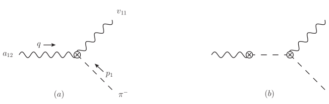
Figure 1: $a)$ Local and $b)$ non-local contributions to the $\langle v_{11}a_{12}\pi^{-}\rangle$ function.

$$G =\frac{1}{q^{2}}\Big{\{}4\,(\alpha_{51}-\alpha_{53})\big{[}\,\epsilon_{v}\cdot q\,\epsilon_{a}\cdot q\,(p_{1}\cdot q)^{2}-\epsilon_{v}\cdot p_{1}\,\epsilon_{a}\cdot q\,(p_{1}\cdot q)^{2}+q^{2}\,\epsilon_{v}\cdot p_{1}\,\epsilon_{a}\cdot p_{1}\,p_{1}\cdot q\,\big{]}$$

$$\quad\quad\ \ +(2\alpha_{50}-\alpha_{51}+\alpha_{52}+\alpha_{53})\,q^{4}\,\epsilon_{v}\cdot\epsilon_{a}\,p_{1}\cdot q+(\alpha_{51}-\alpha_{52}\!-\!\alpha_{53})\,q^{2}\,\epsilon_{v}\cdot q\,\epsilon_{a}\cdot q\,p_{1}\cdot q$$

$$\quad\quad\ \ +(2\alpha_{44}-2\alpha_{51}-\alpha_{52}+3\alpha_{53})\,q^{2}\,\big{[}\,\epsilon_{v}\cdot p_{1}\,\epsilon_{a}\cdot q\,p_{1}\cdot q-q^{2}\,\epsilon_{v}\cdot p_{1}\,\epsilon_{a}\cdot p_{1}\big{]}$$

$$\quad\quad\ \ -(2\alpha_{44}+3\alpha_{51}-2\alpha_{52}-2\alpha_{53})\,q^{2}\,\epsilon_{v}\cdot\epsilon_{a}\,(p_{1}\cdot q)^{2}$$

$$\quad\quad\ \ +(2\alpha_{44}\!-\!\alpha_{51}\!-\!2\alpha_{52}+2\alpha_{53})\,q^{2}\,\epsilon_{v}\cdot q\,\epsilon_{a}\cdot p_{1}\,p_{1}\cdot q$$

$$\quad\quad\ \ +2\,\alpha_{50}\,q^{4}\,\big{[}\,q^{2}\,\epsilon_{v}\cdot\epsilon_{a}-\epsilon_{v}\cdot q\,\epsilon_{a}\cdot p_{1}-\epsilon_{v}\cdot q\,\epsilon_{a}\cdot q\big{]}\Big{\}}\,,$$ (3.15)

up to a global constant factor, and we have also dropped the Dirac delta function with the momentum conservation. The $1/q^{2}$ factor arises from the scalar propagator in diagram Fig. 1a; since we have factored out it globally, the resulting polynomial in the numerator is of order $z_{i}^{4}$ in the kinematic invariants $z_{i}\equiv p_{1}\cdot q,\,p_{1}\cdot\epsilon_{v},\,\dots$. The requirement that the Green function must vanish if a relation between the ${\cal O}(p^{6})$ operators holds requires that the coefficients of all monomials in the numerator vanish. This translates into the following set of conditions for the $\alpha_{i}$:

$$\alpha_{50}=\alpha_{52}=0\quad,\quad\alpha_{51}=\alpha_{53}=-2\alpha_{44}\ .$$ (3.16)

The first condition in (3.16) implies that no relation involving operators ${\cal P}_{50}$ and ${\cal P}_{52}$ can be satisfied by the Green function chosen in this example. Since an operator relation must be true for any Green function we can already conclude that the operators 50 and 52 belong to the minimal basis of the Lagrangian. The second condition in (3.16) translates into the relation ${\cal P}_{44}-2{\cal P}_{51}-2{\cal P}_{53}=0$ being satisfied for this Green function. By analysing other Green functions we shall conclude in Sec. 4 that the later relation is actually part of a larger one involving more terms, that holds exactly for the operators in ${\cal L}_{6}^{\rm SU(2)}$.

Let us now choose a Green function with one field more, for instance $\langle a_{12}a_{21}\pi^{0}\pi^{0}\rangle$, which includes two axial and two pion fields. This example shall give us an idea of the increasing complexity related to diagrams with more legs. Fig. 2 shows the diagrammatic contributions to the corresponding Green function. The pure local term, Fig. 2a, stems from the operators $1-3,36-44$ and $50-53$. The non-local contributions include two different type of diagrams: in Figs. 2b, an axial-$3\pi$ vertex from operators $1-3,36-38$ and $51-53$ of the ${\cal O}(p^{6})$ Lagrangian is combined with the axial-pion vertex from ${\cal L}_{2}^{\rm SU(2)}$ , whereas in Fig. 2c, we need the ${\cal O}(p^{6})$ 4$\pi$ vertices from operators ${\cal P}_{1-3}$.

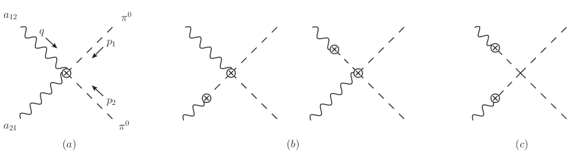
Figure 2: $(a)$ Local and $(b),(c)$ non-local contributions to the $\langle a_{12}a_{21}\pi^{0}\pi^{0}\rangle$ function.

The amplitudes for $\langle a_{12}a_{21}\pi^{0}\pi^{0}\rangle$ depend on $11$ independent Lorentz invariants, namely $p_{1}\cdot p_{2},\,q^{2},\,p_{1}\cdot q,\,p_{2}\cdot q,\,p_{1}\cdot\epsilon_{12},\,p_{2}\cdot\epsilon_{12},\,q\cdot\epsilon_{12},\,p_{1}\cdot\epsilon_{21},\,p_{2}\cdot\epsilon_{21},\,q\cdot\epsilon_{21}$ and $\epsilon_{12}\cdot\epsilon_{21}$, and we have again considered massless pions. The number of monomials of order $p^{6}$ which can be built out of the kinematic invariants is therefore large, and handling the amplitude in order to find out the conditions for the $\alpha_{i}$ requires automatisation. For this task, we have implemented the computation of the tree-level Green functions at ${\cal O}(p^{6})$ and the extraction of the relations for the $\alpha_{i}$ in a Mathematica code. In the case at hand, $\langle a_{12}a_{21}\pi^{0}\pi^{0}\rangle$, one obtains an amplitude with 132 independent monomials in the numerator, whose coefficients yield the equations for $\alpha_{i}$: 50 of these equations are non-trivially identical, but only 10 turn out to be independent. The solution to this system then provides 10 relations among the coefficients $\alpha_{i}$ of the 16 operators that contribute to $\langle a_{12}\,a_{21}\pi^{0}\pi^{0}\rangle$:

$$\alpha_{38}=\alpha_{50}=0\quad,\quad\alpha_{1}=-4\alpha_{2}=\frac{4}{3}\alpha_{3}=\alpha_{36}=-\alpha_{37}\quad,\quad\alpha_{51}=\alpha_{53}$$

$$3\alpha_{1}-2\alpha_{41}-2\alpha_{42}+4\alpha_{43}-4\alpha_{51}=0$$

$$\alpha_{1}+8\alpha_{39}-8\alpha_{40}+6\alpha_{41}+6\alpha_{42}-12\alpha_{43}-8\alpha_{44}=0$$

$$\alpha_{1}+2\alpha_{39}-2\alpha_{40}+\alpha_{41}+\alpha_{42}-2\alpha_{43}-\alpha_{52}=0\ .$$ (3.17)

With these conditions, the function $\langle a_{12}a_{21}\pi^{0}\pi^{0}\rangle$ with an insertion of $(\sum_{i}\alpha_{i}{\cal P}_{i})$ thus becomes

$$\Big{\langle}\alpha_{1}\,\Big{(}\,{\cal P}_{1}-{1\over 4}\,{\cal P}_{2}+{3\over 4}\,{\cal P}_{3}+{\cal P}_{36}-{\cal P}_{37}-{3\over 4}\,{\cal P}_{40}-{\cal P}_{41}-{\cal P}_{42}+{1\over 4}\,{\cal P}_{43}-{\cal P}_{44}+2{\cal P}_{51}+2{\cal P}_{53}\Big{)}$$

$$\quad+\alpha_{39}\,\Big{(}\,{\cal P}_{39}-{\cal P}_{40}-2\,{\cal P}_{41}+{\cal P}_{43}-\,{\cal P}_{44}+2\,{\cal P}_{51}+2\,{\cal P}_{53}\Big{)}\,\Big{\rangle}=0\,,$$ (3.18)

and vanishes for arbitrary values of $\alpha_{1}$ and $\alpha_{39}$. The notation $\langle\dots\rangle$ in (3.18) is short for the matrix element of the linear combination together with the axial-vector and pion fields which defines the Green function. The result (3.18) implies that the two linear relations among the ${\cal P}_{i}$ operators between parenthesis are equal to zero for this particular function. We can proceed in the same way for other Green functions and require a simultaneous vanishing of all of them by solving for the $\alpha_{i}$. The latter is a necessary condition for the existence of a relation between the ${\cal O}(p^{6})$ operators. In the next section we show that the procedure eventually allows for just two relations in the SU(2) case without scalar and pseudo-scalar external fields.

4 SU(2) case with $s=p=0$

$\begin{array}[]{c}\rm Green\\ \rm function\end{array}$	${\cal P}_{i}$	Operator relations
$\langle vv\rangle$	$56$	$\alpha_{56}\!=\!0$
$\langle v\,2\pi\rangle$	$51,53$	${\cal P}_{51}+{\cal P}_{53}=0$
$\langle va\pi\rangle$	$44,50\!-\!53$	$\alpha_{50}\!=\!\alpha_{52}\!=\!0$
		${\cal P}_{44}-2{\cal P}_{51}-2{\cal P}_{53}=0$
$\langle vaa\rangle$	$44,45,$	$\alpha_{50}\!=\!\alpha_{52}\!=\!0$
	$50\!-\!53,55$	$3{\cal P}_{45}+8{\cal P}_{55}=0$
		${\cal P}_{44}-{\cal P}_{45}-2{\cal P}_{51}-2{\cal P}_{53}=0$
$\langle 4\pi\rangle$	$1\!-\!3$	$4{\cal P}_{1}-{\cal P}_{2}+3{\cal P}_{3}=0$
$\langle vv\,2\pi\rangle$	$29\!-\!33,44,$	$\alpha_{50}\!=\!\alpha_{52}\!=\!0$
	$50\!-\!53$	${\cal P}_{29}-{\cal P}_{30}+2{\cal P}_{31}-4{\cal P}_{32}+{\cal P}_{33}-{\cal P}_{44}+2{\cal P}_{51}+2{\cal P}_{53}=0$
$\langle aa\,2\pi\rangle$	$1\!-\!3,36\!-\!44,$	$\alpha_{38}=\alpha_{50}=\alpha_{52}=0$
	$50\!-\!53$	${\cal P}_{39}-{\cal P}_{40}-2{\cal P}_{41}+{\cal P}_{43}-{\cal P}_{44}+2{\cal P}_{51}+2{\cal P}_{53}=0$
		$\begin{array}[]{c}4{\cal P}_{1}-{\cal P}_{2}+3{\cal P}_{3}+4{\cal P}_{36}-4{\cal P}_{37}-4{\cal P}_{39}+{\cal P}_{40}+4{\cal P}_{41}\\ -4{\cal P}_{42}-3{\cal P}_{43}=0\end{array}$
$\langle a\,3\pi\rangle$	$1\!-\!3,36\!-\!38,$	$\alpha_{38}=0$
	$51,53$	4${\cal P}_{1}-{\cal P}_{2}+3{\cal P}_{3}+4{\cal P}_{36}-4{\cal P}_{37}=0$
		${\cal P}_{51}+{\cal P}_{53}=0$
$\langle vva\,\pi\rangle$	$29\!-\!33,44,$	$\alpha_{50}=\alpha_{52}=0$
	$45,50\!-\!53$	$\begin{array}[]{c}{\cal P}_{29}-{\cal P}_{30}+2{\cal P}_{31}-4{\cal P}_{32}+{\cal P}_{33}-{\cal P}_{44}+{\cal P}_{45}\\ +2{\cal P}_{51}+2{\cal P}_{53}=0\end{array}$
$\langle v\,4\pi\rangle$	$1\!-\!3,27\!-\!28$	$\alpha_{38}=0$
	$36\!-\!38,51\!-\!53$	4${\cal P}_{1}-{\cal P}_{2}+3{\cal P}_{3}-6{\cal P}_{27}-14{\cal P}_{28}+4{\cal P}_{36}-4{\cal P}_{37}=0$
		$2{\cal P}_{27}+2{\cal P}_{28}-{\cal P}_{51}-{\cal P}_{53}=0$
$\langle va\,3\pi\rangle$	$1\!-\!3,27\!-\!44,$	$\alpha_{38}=\alpha_{50}=\alpha_{52}=0$
	$50\!-\!53$	${\cal P}_{29}+{\cal P}_{39}=0$
		${\cal P}_{31}+{\cal P}_{32}+{\cal P}_{41}+{\cal P}_{42}=0$
		$\begin{array}[]{c}8{\cal P}_{1}-2{\cal P}_{2}+6{\cal P}_{3}-12{\cal P}_{27}-28{\cal P}_{28}+8{\cal P}_{36}-8{\cal P}_{37}\\ -8{\cal P}_{39}+2{\cal P}_{40}+8{\cal P}_{41}-8{\cal P}_{42}-6{\cal P}_{43}=0\end{array}$
		$\begin{array}[]{c}4{\cal P}_{27}+4{\cal P}_{28}+{\cal P}_{30}-2{\cal P}_{31}+4{\cal P}_{32}-{\cal P}_{33}+{\cal P}_{40}+2{\cal P}_{41}\\ -{\cal P}_{43}+{\cal P}_{44}-2{\cal P}_{51}-2{\cal P}_{53}=0\end{array}$
$\langle 6\pi\rangle$	$1\!-\!3,24\!-\!26$	$4{\cal P}_{1}-{\cal P}_{2}+3{\cal P}_{3}-10{\cal P}_{24}+4{\cal P}_{25}+6{\cal P}_{26}=0$

Table 1: Relations among ${\cal O}(p^{6})$ operators satisfied for each of the Green functions computed. The second column lists the operators that contribute in each case.

As a proof of concept we show in this section how the method described above applies to the two-flavour ChPT Lagrangian in the chiral limit and without additional external scalar or pseudo-scalar sources ($s=p=0$) but $v_{\mu},a_{\mu}\neq 0$. This simplified framework does not lack of phenomenological relevance: it provides a very good approximation to the low-energy interaction of the pions in the presence of electroweak currents, since mass corrections in the $u,d$ quark sector are small and there are no other contributions to the external sources $s$ and $p$ in the Standard Model.

Within this framework, we have computed the Green functions (LABEL:eq:identity) with the generic field content as listed in the first column of Tab. 1. The notation $\langle va\,3\pi\rangle$, for instance, stands for all Green functions involving three pion fields (charged or neutral) and one vector and one axial-vector field component, and similarly for the rest of functions. The second column indicates which ${\cal O}(p^{6})$ operators contribute to the Green functions. The relations among the operators satisfied for each function, obtained as in the examples of Sec. 3 by solving a system of equations for the coefficients $\alpha_{i}$, are then given in the third column. We have not written the equations for the $\alpha_{i}$ for each function except for the cases where they require some of the $\alpha_{i}$ to vanish; the condition $\alpha_{i}=0$ obtained for a given Green function already implies that the corresponding operator ${\cal P}_{i}$ cannot be part of any relation, which is an important information. We note that the relations written in Tab. 1 guarantee that all Green functions with arbitrary charge (or isospin) configuration of the pion and external fields vanish. For a given charge (isospin) channel additional relations among the operators that contribute can exist, which we do not provide in Tab. 1.

The relations satisfied for a set of functions can be obtained by combining the equations for the coefficients $\alpha_{i}$ from each Green function and looking for a compatible solution. From the table one sees that the combination of Green functions $\langle vv\rangle,\,\langle vaa\rangle,\,\langle vv\,2\pi\rangle,\,\langle aa\,2\pi\rangle$, $\langle v\,4\pi\rangle$ and $\langle 6\pi\rangle$ already involve all the operators in the $\mathrm{SU}(2)$ ChPT Lagrangian with $s=p=0$. The fact that operators ${\cal P}_{45}$ and ${\cal P}_{55}$ only appear in $\langle vaa\rangle$ requires a further Green function depending on ${\cal P}_{45}$ in order to fix it completely. That is why the Green function for $\langle vva\pi\rangle$ is also computed. The results for the rest of functions in Tab. 1 is given for completeness; their computation also serves us as a check of the relations found with the minimal set of functions.

Combining the equations for $\alpha_{i}$ found for the different Green functions we get that all the latter vanish provided

$$\alpha_{38}\,=\alpha_{50}\,=\alpha_{52}\,=\alpha_{55}\,=\alpha_{56}=0\,,$$

$$\alpha_{1}\,\Big{(}\,8\,{\cal P}_{1}-2\,{\cal P}_{2}+6\,{\cal P}_{3}-20\,{\cal P}_{24}+8\,{\cal P}_{25}+12\,{\cal P}_{26}-16\,{\cal P}_{28}-3\,{\cal P}_{29}+3\,{\cal P}_{30}-6\,{\cal P}_{31}$$

$$\quad\;\;\;+12\,{\cal P}_{32}-3\,{\cal P}_{33}+8\,{\cal P}_{36}-8\,{\cal P}_{37}-11\,{\cal P}_{39}+5\,{\cal P}_{40}+14\,{\cal P}_{41}-8\,{\cal P}_{42}-9\,{\cal P}_{43}$$

$$\quad\;\;\;+3\,{\cal P}_{44}-3\,{\cal P}_{45}-6\,{\cal P}_{51}-6\,{\cal P}_{53}\Big{)}$$

$$+\; \alpha_{27}\,\Big{(}\,8\,{\cal P}_{27}+8\,{\cal P}_{28}-2\,{\cal P}_{29}+2\,{\cal P}_{30}-4\,{\cal P}_{31}+8\,{\cal P}_{32}-2\,{\cal P}_{33}-2\,{\cal P}_{39}+2\,{\cal P}_{40}$$

$$\quad\;\;\;+4\,{\cal P}_{41}-2\,{\cal P}_{43}+2\,{\cal P}_{44}-2\,{\cal P}_{45}-4\,{\cal P}_{51}-4\,{\cal P}_{53}\Big{)}=0\,,$$ (4.19)

which holds for whatever values of $\alpha_{1}$ and $\alpha_{27}$, meaning that the two linear combinations among the operators ${\cal P}_{i}$ between parenthesis must vanish independently. The relations obtained can be simplified if one uses the second linear combination into the first one, which also allows to compare our result with the additional relation found for the SU(2) case in [6], and with a relation which is known to hold among the ${\cal O}(p^{6})$ operators when the scalar and pseudo-scalar sources are set to zero [8]. In this way we find:

$$4\,{\cal P}_{27}+4\,{\cal P}_{28}-\,{\cal P}_{29}+\,{\cal P}_{30}-2\,{\cal P}_{31}+4\,{\cal P}_{32}-\,{\cal P}_{33} -\,{\cal P}_{39}+\,{\cal P}_{40}+2\,{\cal P}_{41}$$

$$-\,{\cal P}_{43}+\,{\cal P}_{44}-\,{\cal P}_{45}-2\,{\cal P}_{51}-2\,{\cal P}_{53} =0\,,$$ (4.20)

$$8\,{\cal P}_{1}-2\,{\cal P}_{2}+6\,{\cal P}_{3}-20\,{\cal P}_{24}+8\,{\cal P}_{25}+12\,{\cal P}_{26}-12\,{\cal P}_{27} -28\,{\cal P}_{28}+8\,{\cal P}_{36}-8\,{\cal P}_{37}$$

$$-8\,{\cal P}_{39}+2\,{\cal P}_{40}+8\,{\cal P}_{41}-8\,{\cal P}_{42}-6\,{\cal P}_{43} =0\,,$$ (4.21)

that agree with those given in [8] and [6], respectively, once the operators depending on scalar and pseudo-scalar tensor source $\chi$ are neglected in the latter. Since relations (4.20,4.21) were proven algebraically in these references, they are of course satisfied for all Green functions of the form (LABEL:eq:identity). We can moreover state that these are the only two relations between the SU(2) ChPT operators of ${\cal O}(p^{6})$ in the limit $s=p=0$; otherwise any further relation of the form $\sum\alpha_{i}^{\prime}{\cal P}_{i}=0$ would have been obtained from the analysis of the functions of Tab. 1 with our method (let us recall that the vanishing of any Green function with an insertion of $\sum\alpha_{i}^{\prime}{\cal P}_{i}$ is a necessary condition for the existence of the relation). We therefore conclude that the set of minimal operators of the SU(2) ChPT Lagrangian of ${\cal O}(p^{6})$ with scalar and pseudo-scalar sources set to zero reduces from the 27+2 operators initially written down in [5] to 25+2 (note that the contact terms do not take part in any of the relations above). Eqs. (4.20,4.21) can be used to drop two of the 27 basis elements of the basis of [5].

The application of our method to the general two- and three-flavour cases is straightforward.

For SU(2) including scalar and pseudo-scalar sources, if a similar analysis does not yield additional relations to that of Ref. [6], one would conclude that the basis of ${\cal O}(p^{6})$ operators from [5] is minimal up to one term. The case of SU(3) is more involved at the technical level, since we have to consider an octet of pseudo-goldstone bosons and many more Green functions can be built. Starting the analysis of Green functions with less number of fields, one could expect that the space of solutions for the coefficients $\alpha_{i}$ is either very much constrained, and eventually no solution is allowed after computing a few Green functions, or that it actually allows for one (or more) relations among the operators. In the former case one could already conclude that the basis of ${\cal L}_{6}^{\rm SU(3)}$ is minimal. In the latter, one may try to check if the relations found from the analysis of the simpler Green functions also hold at the level of the operators (i.e. for any Green function with an arbitrary number of fields) by using the same algebraic manipulations as in [5], with the great advantage that one would know beforehand the coefficients that the operators participating in the relation must have. The study of the general two- and three-flavour cases with the automated tools developed in this work will be the subject of future investigation.

5 Summary

The large number of low-energy constants in the mesonic chiral Lagrangian of order $p^{6}$ makes their determination by direct comparison with the experiment rather difficult. To simplify this task, one would like to eliminate possible redundancies by establishing the minimal set of independent operators in ${\cal L}_{6}$, that parametrize the rational part of the ${\cal O}(p^{6})$ chiral amplitudes.

We have described in this paper a method to search for additional relations among the basis operators that build the ${\cal O}(p^{6})$ SU$(n)$ chiral Lagrangian. It relies on the computation of tree-level Green functions with insertions of the ${\cal L}_{6}$ operators, which are then required to vanish for an arbitrary kinematic configuration. The method can be used to establish the minimal basis of operators in the Lagrangian. This has been done in the present work for the two-flavour ${\cal O}(p^{6})$ Lagrangian without scalar and pseudo-scalar external sources. For this case we have shown that the original basis of 27 measurable terms plus 2 contact terms written in [5] in the even-intrinsic-parity sector has 25+2 independent terms, where the two additional relations between operators that emerge from our method had been already noticed in the literature [6, 8].

As a next step, the method shall be applied to determine the minimal basis of operators in the SU(2) case with general scalar and pseudo-scalar sources, as well as in SU(3). Furthermore, one can expect that the method extends naturally to other relevant effective actions containing a large number of operators, and in particular to the linear and non-linear effective theories that describe the breaking of the electroweak symmetry.

Acknowledgments

We thank J. Sanz-Cillero for pointing us to the operator relation in Ref. [8] and for his comments on the draft. We also thank G. Ecker for useful communication regarding the functionality of the code Ampcalculator [9], used for cross-checks, and J. Portolés for comments on the draft. MZA wants to thank A.Pich and J. Portolés for helpful discussions. This work is partially supported by MEC (Spain) under grants FPA2007-60323 and FPA2011-23778 and by the Spanish Consolider-Ingenio 2010 Programme CPAN (CSD2007-00042).

6 Appendix

We provide in this appendix the explicit form of the operators in the ${\cal O}(p^{6})$ ChPT Lagrangian in the SU(2) case (2.13) without scalar and pseudo-scalar sources. The expressions are read off from the list given in the appendix C of Ref. [5] by discarding terms containing the $\chi$ tensor.

Besides the chiral tensors already written in Sec. 2, the following building blocks are needed to construct the operators in Tab. 2:

$$h_{\mu\nu}=\nabla^{\mu}u_{\nu}+\nabla^{\nu}u_{\mu}\,,$$

$$f_{\pm}^{\mu\nu}=uF^{\mu\nu}_{L}u^{\dagger}\pm u^{\dagger}F_{R}^{\mu\nu}u\,,\quad\nabla_{\rho}f_{\pm}^{\mu\nu}\,,$$ (6.22)

with the non-abelian field strength tensor built from the right and left external fields,

$$F_{L}^{\mu\nu}=\partial^{\mu}\ell^{\nu}-\partial^{\nu}\ell^{\mu}-i\left[\ell^{\mu},\ell^{\nu}\right]\,,$$

$$F_{R}^{\mu\nu}=\partial^{\mu}r^{\nu}-\partial^{\nu}r^{\mu}-i\left[r^{\mu},r^{\nu}\right]\,$$ (6.23)

and the covariant derivative defined as

$$\nabla_{\mu}X=\partial_{\mu}X+[\Gamma_{\mu},X]\,,$$ (6.24)

where

$$\Gamma_{\mu}=\frac{1}{2}\{u^{{\dagger}}(\partial_{\mu}-ir_{\mu})u+u(\partial_{\mu}-i\ell_{\mu})u^{{\dagger}}\}\,.$$ (6.25)

${\it i}$	${\cal P}_{i}$	Green function
1	$\langle u\hskip-1.29167pt\cdot\hskip-1.29167ptuh_{\mu\nu}h^{\mu\nu}\rangle$	$\langle 4\pi\rangle$
2	$\langle h_{\mu\nu}u_{\rho}h^{\mu\nu}u^{\rho}\rangle$	$\langle 4\pi\rangle$
3	$\langle h_{\mu\nu}\left(u_{\rho}h^{\mu\rho}u^{\nu}+u^{\nu}h^{\mu\rho}u_{\rho}\right)\rangle$	$\langle 4\pi\rangle$
24	$\langle(u\hskip-1.29167pt\cdot\hskip-1.29167ptu)^{3}\rangle$	$\langle 6\pi\rangle$
25	$\langle u\hskip-1.29167pt\cdot\hskip-1.29167ptuu_{\mu}u_{\nu}u^{\mu}u^{\nu}\rangle$	$\langle 6\pi\rangle$
26	$\langle u_{\mu}u_{\nu}u_{\rho}u^{\mu}u^{\nu}u^{\rho}\rangle$	$\langle 6\pi\rangle$
27	i $\langle f_{+\mu\nu}u_{\rho}u^{\mu}u^{\nu}u^{\rho}\rangle$	$\langle v\,4\pi\rangle$
28	i $\langle f_{+\mu\nu}u^{\mu}u\hskip-1.29167pt\cdot\hskip-1.29167ptuu^{\nu}\rangle$	$\langle v\,4\pi\rangle$
29	$\langle u\hskip-1.29167pt\cdot\hskip-1.29167ptuf_{+\mu\nu}f_{+}^{\mu\nu}\rangle$	$\langle vv\,2\pi\rangle$
30	$\langle f_{+\mu\nu}u_{\rho}f_{+}^{\mu\nu}u^{\rho}\rangle$	$\langle vv\,2\pi\rangle$
31	$\langle f_{+\mu\nu}f_{+}^{\mu\rho}u^{\nu}u_{\rho}\rangle$	$\langle vv\,2\pi\rangle$
32	$\langle f_{+\mu\nu}f_{+}^{\mu\rho}u_{\rho}u^{\nu}\rangle$	$\langle vv\,2\pi\rangle$
33	$\langle f_{+\mu\nu}\left(u_{\rho}f_{+}^{\mu\rho}u^{\nu}+u^{\nu}f_{+}^{\mu\rho}u_{\rho}\right)\rangle$	$\langle vv\,2\pi\rangle$
36	$\langle f_{-\mu\nu}\left(h^{\nu\rho}u_{\rho}u^{\mu}+u^{\mu}u_{\rho}h^{\nu\rho}\right)\rangle$	$\langle a\,3\pi\rangle$
37	$\langle f_{-\mu\nu}h^{\nu\rho}\rangle\langle u^{\mu}u_{\rho}\rangle$	$\langle a\,3\pi\rangle$
38	$\langle f_{-\mu\nu}\left(u^{\mu}h^{\nu\rho}u_{\rho}+u_{\rho}h^{\nu\rho}u^{\mu}\right)\rangle$	$\langle a\,3\pi\rangle$
39	$\langle u\hskip-1.29167pt\cdot\hskip-1.29167ptuf_{-\mu\nu}f_{-}^{\mu\nu}\rangle$	$\langle aa\,2\pi\rangle$
40	$\langle f_{-\mu\nu}u_{\rho}f_{-}^{\mu\nu}u^{\rho}\rangle$	$\langle aa\,2\pi\rangle$
41	$\langle f_{-\mu\nu}f_{-}^{\mu\rho}u^{\nu}u_{\rho}\rangle$	$\langle aa\,2\pi\rangle$
42	$\langle f_{-\mu\nu}f_{-}^{\mu\rho}u_{\rho}u^{\nu}\rangle$	$\langle aa\,2\pi\rangle$
43	$\langle f_{-\mu\nu}\left(u_{\rho}f_{-}^{\mu\rho}u^{\nu}+u^{\nu}f_{-}^{\mu\rho}u_{\rho}\right)\rangle$	$\langle aa\,2\pi\rangle$
44	i $\langle f_{+\mu\nu}[f_{-}^{\nu\rho},h^{\mu}_{\rho}]\rangle$	$\langle va\,\pi\rangle$
45	i $\langle f_{+\mu\nu}[f_{-}^{\nu\rho},f_{-\rho}^{\mu}]\rangle$	$\langle vaa\rangle$
50	$\langle\nabla_{\rho}f_{-\mu\nu}\nabla^{\rho}f_{-}^{\mu\nu}\rangle$	$\langle aa\rangle$
51	i $\langle\nabla_{\rho}f_{+\mu\nu}[h^{\mu\rho},u^{\nu}]\rangle$	$\langle v\,2\pi\rangle$
52	i $\langle\nabla^{\mu}f_{+\mu\nu}[f_{-}^{\nu\rho},u_{\rho}]\rangle$	$\langle va\,\pi\rangle$
53	i $\langle\nabla^{\mu}f_{+\mu\nu}[h^{\nu\rho},u_{\rho}]\rangle$	$\langle v\,2\pi\rangle$
contact terms
55	i $\langle F_{L\mu\nu}F_{L}^{\mu\rho}F_{L\rho}^{\nu}\rangle+L\rightarrow R$	$\langle vaa\rangle$
56	$\langle D_{\rho}F_{L\mu\nu}D^{\rho}F_{L}^{\mu\nu}\rangle+L\rightarrow R$	$\langle vv\rangle$

Table 2: ${\cal O}(p^{6})$ operators for $\mathrm{SU}(2)$ with $s=p=0$, in the basis of [5]. The label in the first column refers to the SU(2) numbering scheme used in the latter reference. The last column indicates the simplest Green function to which the operator contributes.

References

- [1] S. Weinberg, Physica A 96 (1979) 327.
- [2] J. Gasser and H. Leutwyler, Annals Phys. 158 (1984) 142.
- [3] J. Gasser and H. Leutwyler, Nucl. Phys. B 250 (1985) 465.
- [4] H. W. Fearing and S. Scherer, Phys. Rev. D 53 (1996) 315 [hep-ph/9408346].
- [5] J. Bijnens, G. Colangelo and G. Ecker, JHEP 9902 (1999) 020 [hep-ph/9902437].
- [6] C. Haefeli, M. A. Ivanov, M. Schmid and G. Ecker, arXiv:0705.0576 [hep-ph].
- [7] C. Arzt, Phys. Lett. B 342 (1995) 189 [hep-ph/9304230].
- [8] P. Colangelo, J. J. Sanz-Cillero and F. Zuo, JHEP 1211 (2012) 012 [arXiv:1207.5744 [hep-ph]].
- [9] http://homepage.univie.ac.at/Gerhard.Ecker/CPT-amp.html