Temperature control of thermal radiation from heterogeneous bodies

Abstract

We demonstrate that recent advances in nanoscale thermal transport and temperature manipulation can be brought to bear on the problem of tailoring thermal radiation from compact emitters. We show that wavelength-scale composite bodies involving complicated arrangements of phase-change chalcogenide (GST) glasses and metals or semiconductors can exhibit large emissivities and partial directivities at mid-infrared wavelengths, a consequence of temperature localization within the GST. We consider multiple object topologies, including spherical, cylindrical, and mushroom-like composites, and show that partial directivity follows from a complicated interplay between particle shape, material dispersion, and temperature localization. Our calculations exploit a recently developed fluctuating–volume current formulation of electromagnetic fluctuations that rigorously captures radiation phenomena in structures with both temperature and dielectric inhomogeneities.

The ability to control thermal radiation over selective frequencies and angles through complex materials and nanostructured surfaces Greffet and Henkel (2007) has enabled unprecedented advances in important technological areas, including remote temperature sensing Masuda et al. (1988), incoherent sources Ilic and Soljačić (2014); Rinnerbauer et al. (2014), and energy-harvesting Fan (2014); Bermel et al. (2011); Florescu et al. (2007). Recent progress in the areas of temperature management and thermal transport at sub-micron scales can play a significant (and largely unexplored) role in the design of specially engineered radiative structures that combine both photonic and phononic design principles Cahill et al. (2003, 2014).

In this letter, we describe a fluctuating–volume current (FVC) formulation of electromagnetic (EM) fluctuations that enables fast and accurate calculations of thermal radiation from complex structures with non-uniform temperature and dielectric properties. We demonstrate that when selectively heated, wavelength-scale composite bodies—complicated arrangements of phase-change materials and metals or semiconductors—can exhibit large temperature gradients and partially directed emission at infrared wavelengths. For instance, micron-scale chalcogenide (GST) hemispheroids coated with titanium or silicon-nitride shells [Fig. 1] and resting on a low-index, transparent substrate can exhibit large emissivity and $\gtrsim 80\%$ partial directivity—redirecting light away from the metallic or toward the semiconducting shell—when heated to $870$ K by highly conductive 2D materials at the GST–substrate interfaces. The interplay of geometry and temperature localization allows such composite infrared thermal antennas to not only enhance but also selectively emit and absorb light in specific directions. We show that other designer bodies, including mushroom-like particles and coated cylinders [Fig. 3], can also exhibit large partial directivity, in contrast to situations involving homogeneous bodies or uniform temperature distributions which lead to nearly isotropic emission. Our predictions are based on accurate numerical solutions of the conductive heat equation and Maxwell’s equations, which not only incorporate material dispersion but also account for the existence of thermal and dielectric gradients at the scale of the EM wavelength, where ray optical descriptions are inapplicable.

Attempts to obtain unusual thermal radiation patterns have primarily relied on Bragg scattering and related interference effects in nanostructured surfaces Greffet and Henkel (2007), including photonic gratings De Zoysa et al. (2012); Wang et al. (2014); Florescu et al. (2007), metasurfaces Greffet et al. (2002); Marquier et al. (2004); Joulain et al. (2005); Hesketh et al. (1988); Narayanaswamy and Chen (2005); Marquier et al. (2015); Kleiner et al. (2012); Ribaudo et al. (2013), multilayer structures Kollyukh et al. (2003); Ben-Abdallah (2004); Drevillon et al. (2011); Wang et al. (2011), and sub-wavelength metamaterials Lee et al. (2008); Fu and Zhang (2009); Liu et al. (2011a); Bermel et al. (2011); Liu et al. (2011b). Related ideas can also be found in the context of fluorescence emission, where directivity is often achieved by employing metallic objects (e.g. plasmonic antennas) to re-direct emission from individual dipolar emitters via gratings Curto et al. (2010); Kosako et al. (2010) or by localizing fluorescent molecule(s) to within some region in the vicinity of an external scatterer Teperik and Degiron (2011); Thomas et al. (2004); Li et al. (2007); Vandenbem et al. (2009, 2010); Mohammadi et al. (2008). Matters become complicated when the emission is coming from random sources distributed within a wavelength-scale object, as is the case for thermal radiation, because the relative contribution of current sources to radiation in a particular direction is determined by both the shape and temperature distribution of the object. Optical antennas have recently been proposed as platforms for control and design of narrowband emitters Schuller et al. (2009); Novotny and Van Hulst (2011), though predictions of large directivity continue to be restricted to periodic structures. While there is increased focus on the study of light scattering from subwavelength particles and microwave antennas (useful for radar detection Balanis (2005), sensing Taminiau et al. (2007), and color routing Alavi Lavasani and Pakizeh (2012); Shegai et al. (2011)), similar ideas have yet to be translated to the problem of thermal radiation from compact, wavelength-scale objects, whose radiation is typically quasi-isotropic Greffet and Henkel (2007). Here, we show that temperature manipulation in composite particles could play an important role in the design of coherent thermal emitters.

Temperature gradients can arise near the interface of materials with highly disparate thermal conductivities Cahill et al. (2014). Although often negligible at macroscopic scales Balandin (2011), recent experiments reveal that the presence of thermal boundary resistance  Reifenberg et al. (2008); Marconnet et al. (2013) (including intrinsic and contact resistance Stevens et al. (2007)) in nanostructures together with large dissipation can enable temperature localization over small distances Balandin (2011). Such temperature control has been recently investigated in the context of metallic nanospheres immersed in fluids Merabia et al. (2009), graphene transistors Islam et al. (2013), nanowire resistive heaters Yeo et al. (2014), AFM tips King et al. (2013), and magnetic contacts Petit-Watelot et al. (2012). With the exception of a few high–symmetry structures, e.g. spheres Dombrovsky (2000) and planar films Wang et al. (2011), however, calculations of thermal radiation from wavelength-scale bodies have been restricted to uniform-temperature operating conditions, exploiting Kirchoff’s law Luo et al. (2004); Wang et al. (2011) to obtain radiative emission via simple scattering calculations. The presence of temperature and dielectric inhomogeneities in objects with features at the scale of the thermal and EM wavelengths call for alternative theoretical descriptions.

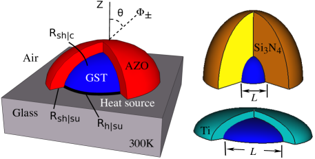
Figure 1: Schematic of representative composite bodies comprising GST (blue) hemispheroids coated with Ti (green), AZO (red), or Si₃N₄ (orange) shells, and resting on a low-index, transparent substrate in contact with a heat reservoir at 300 K. The GST is heated from below by a conductive 2D material (e.g. a carbon-nanotube wall or graphene sheet), leading to temperature gradients within the structure. The presence of boundary resistance at material interfaces is captured by effective (intrinsic and contact) thermal resistances $R_{\mathrm{th}}$.

Formulation.— In what follows, we present a brief derivation of our FVC formulation of thermal radiation, with validations and details of its numerical implementation described in a separate manuscript Polimeridis et al. (2015). Our starting point is the VIE formulation of EM scattering Polimeridis et al. (2014), describing scattering of an incident, 6-component electric ($\mathbf{E}$) and magnetic ($\mathbf{M}$) field $\phi_{\rm inc}=(\mathbf{E};\mathbf{H})$ from a body described by a spatially varying $6\times 6$ susceptibility tensor $\chi(\mathbf{x})$. (For convenience, we omit the frequency $\omega$ dependence of material properties, currents, fields, and operators, and also define $\chi$ to be the susceptibility relative to the background medium.) Given a 6-component electric ($\mathbf{J}$) and magnetic ($\mathbf{M}$) dipole source $\sigma=(\mathbf{J};\mathbf{M})$, the incident field is obtained via a convolution ($\star$) with the $6\times 6$ homogeneous Green’s function (GF) of the ambient medium $\Gamma(\mathbf{x},\mathbf{y})$, such that $\phi_{\mathrm{inc}}=\Gamma\star\sigma=\int d^{3}\mathbf{y}\Gamma(\mathbf{x},\mathbf{y})\sigma(\mathbf{y})$. Exploiting the volume equivalence principle Polimeridis et al. (2014), the unknown scattered fields $\phi_{\rm sca}=\Gamma\star\xi$, can also be expressed via convolutions with $\Gamma$, except that here $\xi=-i\omega\chi\phi$ are the (unknown) bound currents in the body, related to the total field inside the body $\phi=\phi_{\mathrm{inc}}+\phi_{\mathrm{sca}}$ through $\chi$. Writing Maxwell’s equations in terms of the incident and induced currents,

$$\xi+i\omega\chi(\Gamma\star\xi)=-i\omega\chi(\Gamma\star\sigma),$$ (1)

one obtains $\xi$ in terms of the incident source $\sigma$.

Consider a Galerkin discretization of Eq. 1 via expansions of the current sources $\sigma(\mathbf{x})=\sum_{n}s_{n}b_{n}(\mathbf{x})$ and $\xi(\mathbf{x})=\sum_{n}x_{n}b_{n}(\mathbf{x})$ in a convenient, orthonormal basis $\{b_{n}\}$ of $N$ 6-component vectors, with vector coefficients $s$ and $x$, respectively. The resulting matrix expression has the form $x+s=Ws$, where $({W}^{-1})_{m,n}=\langle b_{m},b_{n}+i\omega\chi(\Gamma\star b_{n})\rangle$ is known as the VIE matrix and $\langle,\rangle$ denotes the standard conjugated inner product. Poynting’s theorem implies that the far-field radiation flux $\Phi=\frac{1}{2}\operatorname{Re}\int d^{3}\mathbf{x}\,(\mathbf{E}^{*}\times\mathbf{H})$ due to $\sigma$,

$$\Phi_{\sigma} =-\frac{1}{2}\operatorname{Re}\xi^{*}\phi=-\frac{1}{2}\operatorname{Re}(\xi+\sigma)^{*}\Gamma\star(\xi+\sigma)$$

$$=-\frac{1}{2}(x+s)^{*}\operatorname{sym}G(x+s)=-\frac{1}{2}s^{*}W^{*}\operatorname{sym}GWs$$

$$=-\frac{1}{2}\text{Tr }\left[(s^{*}s)W^{*}\operatorname{sym}GW\right]$$

where $s^{*}s$ and $G$ are both $N\times N$ matrices and ${G}_{mn}=\langle b_{m},\Gamma\star b_{n}\leavevmode\nobreak\ \rangle$ are the elements of the so-called “Green” matrix. Thermal radiation from such a body follows from the cumulative flux contributions of a collection of incoherent sources distributed throughout its volume Polimeridis et al. (2015), obtained by a thermodynamic, ensemble-average $\Phi=\langle\Phi_{\sigma}\rangle$ over all $\sigma$ and polarizations. It follows that the total radiation is given by:

$$\Phi=-\frac{1}{2}{\rm Tr}\left[{C}{W}^{\ast}\operatorname{sym}{{G}}{W}\right],$$ (2)

where we have defined the current–current correlation matrix $C$, whose elements ${C}_{mn}=\langle{s_{m}}{s_{n}}^{\ast}\rangle=\int\int d^{3}\mathbf{x}d^{3}\mathbf{y}\,b_{m}^{\ast}(\mathbf{x})\langle\sigma(\mathbf{x})\sigma^{\ast}(\mathbf{y})\rangle b_{n}(\mathbf{y})$. The correlation functions satisfy a well-known fluctuation–dissipation theorem (FDT) Landau et al. (1960), $\langle\sigma_{i}(\mathbf{x},\omega)\sigma_{j}^{\ast}(\mathbf{y},\omega)\rangle=\frac{4}{\pi}\omega\operatorname{Im}\chi(\mathbf{x},\omega)\Theta(\mathbf{x},\omega)\delta(\mathbf{x}-\mathbf{y})\delta_{ij}$, relating current fluctuations to the dissipative $\sim\operatorname{Im}\chi$ and thermodynamic properties of the underlying materials. Here, $\Theta(\mathbf{x},\omega)=\hbar\omega/(e^{\hbar\omega/k_{\rm B}T(\mathbf{x})}-1)$ is the Planck distribution at the local temperature $T(\mathbf{x})$ Rodriguez et al. (2013). In addition to the total flux, it is also desirable to obtain the angular radiation pattern from bodies, which can be straightforwardly obtained by introducing the far-field Green matrix ${G}_{\infty}^{\rm E\ast}=\langle b_{m},Q\Gamma_{\infty}^{\rm E}\star b_{n}\rangle$, based on the $3\times 6$ GF $\Gamma_{\infty}^{\rm E}(\mathbf{x},\mathbf{y})$ which maps currents to far-field electric fields and the $3\times 3$ tensor $Q$ mapping Cartesian to spherical coordinates (azimuthal and polar angles) Balanis97. Following a similar derivation, the angular radiation flux in a given direction will be given by:

$$U=\frac{k^{2}Z}{2(4\pi)^{2}}{\rm Tr}\left[{C}\,{W}^{\ast}({G}_{\infty}^{\rm E\ast}{G}_{\infty}^{\rm E}){W}\right],$$ (3)

where $k=\omega/c$ and $Z=\sqrt{\mu_{0}/\varepsilon_{0}}$ is the wave impedance of the background medium. Equation 3 can be employed to calculate emission from arbitrarily shaped bodies with spatially varying dielectric and temperature properties—unlike previous scattering-matrix and surface-integral equation formulations of thermal radiation Rodriguez et al. (2013), the FVC scattering unknowns are volumetric currents. Furthermore, when considered as a numerical method as we do below, the corresponding basis functions can be chosen to be localized “mesh” elements Johnson (2011), allowing resolution to be employed where needed Polimeridis et al. (2015).

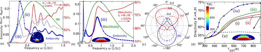
Figure 2: Spectral emissivity $\epsilon(\omega)=\Phi(\omega)/\Phi_{\mathrm{BB}}(\omega)$ (blue dots) from composite bodies comprising Ge₂Sb₂Te₅ (GST) hemispheroids coated with either (a) Si₃N₄ or (b) Ti shells, under heating scenarios (ii) and (iii), respectively (see text). The dashed blue line in (a) shows $\epsilon$ for the Si₃N₄ structure under heating scenario (iii). Both structures rest on a low-index substrate (shown schematically in Fig. 1) and are heated from the GST–substrate interface by a 2D thin-film conductor, reaching an interface temperature $T_{\mathrm{GST}}=870$ K; the temperature profiles $T(\mathbf{x})$ are shown as insets. $\epsilon$ is defined as the ratio of the thermal flux $\Phi(\omega)$ from each body normalized to the flux $\Phi_{\mathbf{BB}}=\frac{A}{4\pi^{2}}(\omega/c)^{2}\Theta(\omega,T)$ from a corresponding black body of same area $A$ and uniform temperature $T=870$ K (green lines, arbitrary units). Also shown are the partial directivities $\eta_{\pm}=\Phi_{\pm}/\Phi$ (red line), defined as the ratios of the outgoing flux into the upper/lower hemisphere $\Phi_{\pm}=2\pi\int_{\mp\pi/2}^{\pi\mp\pi/2}d\theta\,\Phi(\omega,\theta)$ to the total flux, where $\theta$ is defined in Fig. 1. (c) Angular radiation intensity $U(\theta)$ for the structures in (a) (solid red line) or (b) (solid blue line) as well as under heating scenario (v), corresponding to uniform temperature distributions (dashed lines). (d) Total (frequency integrated) downward partial directivity $P_{-}=H_{-}/H$ as a function of $T_{\mathrm{GST}}$, where $H_{-}=\int_{0}^{\infty}d\omega\,\Phi_{-}(\omega)$ and $H=\int_{0}^{\infty}d\omega\,\Phi(\omega)$, for the Ti structure under different heating conditions, corresponding to multiple degrees of temperature localization in the GST (see text).

Results.— In what follows, we explore radiation from composite bodies comprised of chalcogenide Ge₂Sb₂Te₅ (GST) alloys and metals or semiconductors. To begin with, we consider micron-scale GST hemispheroids coated with either titanium (Ti) or silicon-nitride (Si₃N₄) shells, depicted in Fig. 1 and described in detail in [SM]. The structures rest on a low-index ($\varepsilon\approx 1$) transparent substrate which not only provides mechanical support but also a means of dissipating heat away from the structure; the bottom of the substrate is assumed to be in contact with a 300 K heat reservoir while surfaces exposed to vacuum satisfy adiabatic boundary conditions ($\nabla T\cdot\mathbf{\hat{n}}=0$). When heated by a highly conductive 2D material (e.g. carbon nanotube wall or graphene sheet) at the GST–substrate interface, such a structure can exhibit large temperature gradients within the core, a consequence of boundary resistance between the various interfaces and rapid heat dissipation in the highly conductive shells Reifenberg et al. (2008); Xiong et al. (2009); Liang et al. (2012). To model the corresponding steady-state temperature distribution $T(\mathbf{x})$, we solve the heat-conduction equation via COMSOL , including the full temperature-dependent thermal conductivity $\kappa(T)$ of the GST Lyeo et al. (2006). Note that even at large temperatures, $\kappa_{\mathrm{GST}}(800\leavevmode\nobreak\ \mathrm{K})\ll\kappa_{\mathrm{Ti,Si_{3}N_{4}}}(300\leavevmode\nobreak\ \mathrm{K})\gtrsim 20\leavevmode\nobreak\ W/\mathrm{m}\mathrm{K}$. The existence of (intrinsic and contact) boundary resistance at this scale is taken into account by the introduction of effective resistances $R_{\mathrm{sh|c}}$, $R_{\mathrm{h|su}}$, and $R_{\mathrm{sh|su}}$, at the interfaces between shell–GST, heater–substrate, and shell–substrate, respectively [SM]. Figure 2(d) shows $T(\mathbf{x})$ throughout the Ti structure when the GST–substrate interface is heated to $T_{\mathrm{GST}}=870$ K (approaching the GST melting temperature Tsafack et al. (2011)), and under various operating conditions. Specifically, we consider $R_{\mathrm{sh|su}}=10^{-8}\mathrm{m}^{2}W/$K and $R_{\mathrm{sh|c}}=R_{\mathrm{h|su}}=R_{th}$, where {(i), (ii), (iii)} correspond to typical values of $R_{th}=\{0.5,1,2\}\times 10^{-7}\mathrm{m}^{2}W/$K while (iv) $R_{th}=\infty$ and (v) $R_{th}=0$ describe extreme situations involving either perfect temperature localization in the GST or uniform temperature throughout the structure, respectively.

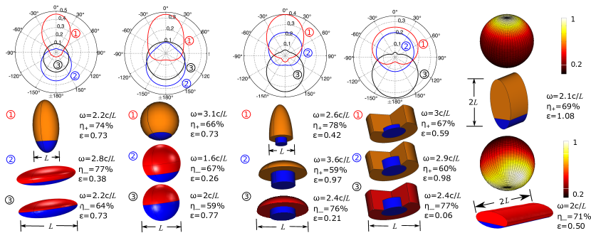
Figure 3: Angular radiation intensity $U(\theta)$ for a variety of heterogeneous bodies—composite GST(blue), AZO (red), and Si₃N₄ (orange) ellipsoids, spheres, mushrooms and cylinders—at selected frequencies $\omega$. The temperature of the GST is held at 870 K while that of other materials is fixed at 300 K. $\epsilon$ and $\eta_{\pm}$ denote the emissivity and partial directivities in the upper/lower hemispheres, defined (along with $\theta$) in Fig. 1 and in the text. Polar (3D) plots are normalized by the total flux.

Given $T(\mathbf{x})$ and the dielectric properties of the bodies Shportko et al. (2008); Li et al. (2008); Mash and Motulevich (1973); Kischkat et al. (2012), the flux can be obtained via Eq. 3. Due to temperature gradients and phase transitions in the GST Lyeo et al. (2006), its dielectric response $\varepsilon_{\mathrm{GST}}(T(\mathbf{x}),\omega)$ consists of continuously varying rather than piece-wise constant regions [SM]; our FVC method, however, can handle arbitrarily varying $\varepsilon(\mathbf{x})$ and $T(\mathbf{x})$. The choice of materials, shapes, and dimensions of the hemispheroids ensure the existence of geometric resonances near the thermal wavelength $\lambda_{T}\approx 5.8\mu$m, corresponding to the peak of the blackbody spectrum at $870$ K. In this wavelength regime, $\varepsilon_{\mathrm{GST}}\approx 30+5i$ Li et al. (2008); Shportko et al. (2008), $\varepsilon_{\mathrm{Ti}}\approx-100+80i$ Mash and Motulevich (1973), and $\varepsilon_{\mathrm{Si_{3}N_{4}}}\approx 5+0.1i$ Kischkat et al. (2012), enabling significant Purcell enhancement and emission Bohren and Huffman (2008). Figure 2 shows the emissivity and partial directivity of the (a) Si₃N₄ and (b) Ti structures, along with their corresponding $T(\mathbf{x})$ (insets) under heating scenarios (ii) or (iii), respectively, and for $T_{\mathrm{GST}}=870$ K. The emissivity $\epsilon(\omega)=\Phi(\omega)/\Phi_{\mathrm{BB}}(\omega)$ (blue dots) is defined as the ratio of the thermal flux $\Phi(\omega)$ from each object to that of a blackbody $\Phi_{\mathrm{BB}}(\omega)=\frac{A}{4\pi^{2}}(\omega/c)^{2}\Theta(\omega,T)$ of the same surface area $A$ and uniform $T=870$ K (green lines); the partial directivity $\eta_{\pm}=\Phi_{\pm}/\Phi$ (red lines) is defined as the ratio of the flux into the upper/lower hemisphere $\Phi_{\pm}(\omega)=2\pi\int_{\mp\pi/2}^{\pi\mp\pi/2}d\theta\,\Phi(\omega,\theta)$, to the total flux $\Phi$, where $\theta$ is defined with respect to the $+\hat{z}$ axis [Fig. 1]. Note that although $\epsilon$ exhibits multiple peaks, its magnitude ($\epsilon\lesssim 0.2$) is limited by material losses ($\operatorname{Im}\varepsilon\lesssim\operatorname{Re}\varepsilon$) in this frequency range Bohren and Huffman (2008); larger $\epsilon$ can likely be optained with further design and/or material combinations.

We find that $\eta$ increases sharply as the system transitions from quasistatic to wavelength-scale behavior (in contrast to $\epsilon$ which exhibits gradual variations, except near a resonance). At small $\omega L/c\ll 1$, the emission is highly quasi-isotropic (as expected from a randomly polarized dipolar emitter Greffet et al. (2002)), becoming increasingly asymmetric as $\omega L/c\gtrsim 1$. Essentially, with the help of the curvature Yu et al. (2013), the Si₃N₄ and Ti shells redirect radiation upwards or downwards, enabling strong coherent interference between the radiated and scattered fields of dipole emitters within the GST, making the design of the temperature profile an essential ingredient for achieving large $\eta$. Figure 2(c) shows the angular radiation intensity $U(\theta)$ of the Si₃N₄ (red) and Ti (blue) structures at selected frequencies and under two of the above-mentioned heating conditions, corresponding to either (ii) partial temperature localization in the GST (solid lines) or (v) uniform temperature throughout the bodies (dashed lines). The dramatically different radiation patterns and significantly smaller $\eta$ under (v) belie the fact that dipole emitters inside the GST contribute larger partial directivity compared to those in the shell, which tend to radiate quasi-isotropically and dominate $\epsilon$.

To illustrate the non-negligible impact of $T(\mathbf{x})$ on the total radiation of the bodies, Fig. 2(d) shows the frequency-integrated, downward partial directivity $P_{-}=H_{-}/H$ of the Ti structure under different $T_{\mathrm{GST}}$ and heating scenarios, where $H_{-}=\int_{0}^{\infty}d\omega\,\Phi_{-}(\omega)$ and $H=\int_{0}^{\infty}d\omega\,\Phi(\omega)$. As expected, $P_{-}$ grows with increasing temperature localization in the GST, and remains almost constant $\approx 0.55$ under uniform temperature conditions. Such an increase in partial directivity, however, comes at the expense of decreasing $\epsilon$ (not shown) due to the increasingly dominant role of larger frequencies. At large $\omega$ or for large bodies (where ray optics becomes valid), material losses severely diminish $\epsilon$. Not surprisingly, the design criteria of such wavelength-scale emitters differs significantly from that of large-scale bodies (where Kirchoff’s law is valid Weinstein (1960)). For instance, while larger $\eta$ can be obtained in the ray-optics limit by increasing the shell thickness of each structure relative to the GST dimensions (thereby enhancing extraction/reflections of radiation from the core), optimal $\eta$ at a fixed frequency $\omega L/c\sim 1$ occur at specific shell thicknesses, determined by the shape and materials of the bodies. Planar structures can also yield highly directional emission when subject to inhomogeneous temperature distributions Wang et al. (2011), but require significantly larger boundary resistance (heating power) and offer limited degrees of freedom for controlling emission. Compared to large-scale or planar radiators, wavelength-scale composite bodies not only provide a high degree of temperature tunability, but also enable simultaneous enhancement in $\eta$ and $\epsilon$, even potentially exceeding the ray-optical, blackbody limit Bohren and Huffman (2008).

Figure 3 shows the radiation pattern of other heterogeneous structures (ellipsoids, spheres, mushroom-like particles, and cylindrical composites), depicted schematically in the figure with blue/red/orange denoting GST/AZO/Si₃N₄ materials. Their shapes and dimensions are detailed in [SM]. For simplicity, we consider emission at selected frequencies and under heating scenario (iv), corresponding to perfect temperature localization in the GST. As expected, the design criteria for achieving large $\eta$ differs depending on the choice of materials, with GST–Si₃N₄ composites favoring large-curvature prolate bodies Yu et al. (2013) and GST–AZO composites favoring oblate structures that provide higher reflections.

Concluding remarks.— The predictions above provide proof of principle that combining conductive and radiative design principles in wavelength-scale structures can lead to unusual thermal radiative effects. Together with our FVC formalism, they motivate the need for rigorous theoretical calculations of thermal emission that account for existence of temperature and dielectric gradients in micron-scale, structured surfaces, an issue that is especially relevant to thermal metrology Fischer and Fellmuth (2005). The FVC framework not only enables fast and accurate calculations, but also for techniques from microwave antenna design and related fields to be carried over over to problems involving infrared thermal radiation. Although the focus of this work is on thermal radiation, similar ideas and techniques are applicable to problems involving fluorescence or spontaneous emission where, rather than controlling the temperature profile, it is possible to localize and control the sources of emission via doping Banaei and Abouraddy (2013) or judicious choice of incident laser light Le Ru and Etchegoin (2008).

We are grateful to Bhavin Shastri for very helpful comments. This work was supported in part by the National Science Foundation under Grant No. DMR-1454836.

Supplemental Materials: Temperature control of thermal radiation from heterogeneous bodies

Below, we provide details of the geometric and material properties of the composite bodies described in the main text, along with addition discussion of the parameters and assumptions of the heating schemes leading to temperature gradients.

I Geometry and material parameters

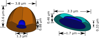
Figure S1: Shape parameters describing the Si₃N₄ (left) and Ti (right) composite hemispheroids explored in Fig. 2 of the main text. Blue, orange, and green colors denote GST, Si₃N₄, Ti, respectively.

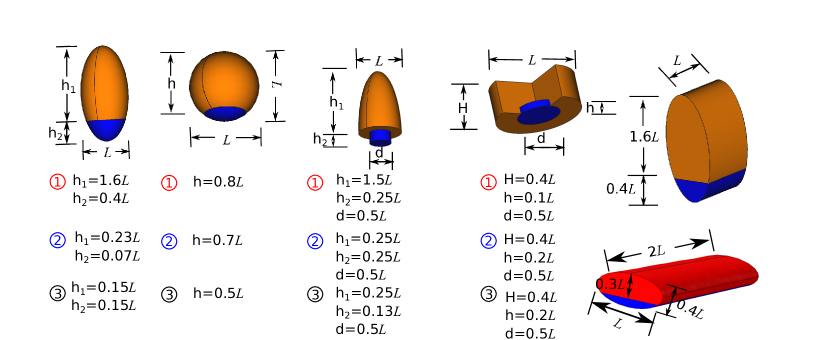
Figure S4: Parameter descriptions for the bodies associated with Fig. 3 of the main text.

Figure S1 provides schematics of the Si₃N₄ (left) and Ti (right) hemispheroid composites explored in Fig. 2 of the text, along with the corresponding geometrical parameters. In particular, the Si₃N₄ and Ti shells have long (short) semi-axes $2.6(1.9)\mu$m and $1.2(0.46)\mu$m, respectively; the chalcogenide (GST) cores have long (short) semi-axes of $0.88(0.63)\mu$m and $0.83(0.33)\mu$m, respectively. As noted in the text, these values are chosen in order to enhance the emissivity and partial directivity of the structures. Figure S4 provides the size and dimensions of the various geometries explored in Fig. 3 of the text.

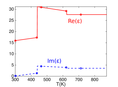
Figure S2: Real (solid red) and imaginary (dashed blue) permittivity $\varepsilon_{\mathrm{GST}}(T,\lambda)$ of a bulk GST glass at $\lambda=5.8\mu$m, obtained via simple linear interpolation of experimental data at multiple temperatures (circles).

The Ge₂Sb₂Te₅ alloy is a phase-change chalcogenide glass that exhibits a large thermo-optic effect Rudé et al. (2013) and three possible (amorphous, cubic, and hexagonal) phases corresponding to transition temperatures of 438 K (separating the amorphous and cubic phases) and 623 K (separating the cubic and hexagonal phases) Li et al. (2008); Xiong et al. (2009). Because there are yet no experimental characterizations or semi-analytical models of the dielectric dispersion $\varepsilon_{\mathrm{GST}}(\omega,T)$ of the GST from $300$ K to its melting point $870$ K Tsafack et al. (2011), we instead model the dispersion via a simple linear-interpolated fit of available experimental data at five different temperatures (spanning amorphous, cubic and hexagonal phases) Li et al. (2008); Shportko et al. (2008). Figure S2 shows both the real (red solid line) and imaginary (blue dashed line) parts of $\varepsilon_{\mathrm{GST}}$ at a single wavelength $\lambda=5.8\mu$m over this temperature range (with circles denoting experimental data). Together with the temperature profiles of the structures $T(\mathbf{x})$ and dispersion relations of Ti Mash and Motulevich (1973), Si₃N₄ Kischkat et al. (2012), and AZO Kim et al. (2012), this provides all of the information needed to perform the calculations of thermal radiation from the bodies of Fig. 2 in the main text. On the other hand, Fig.  3 of the main text explores single-frequency radiation from bodies with piece-wise constant temperature profiles (constant $T=870$ K in the GST and $300$ K in the remaining regions), which allows us to employ typical permittivity values for these materials at mid-infrared wavelengths; specifically, we choose $\varepsilon_{\mathrm{GST}}=30+10i$ Shportko et al. (2008), $\varepsilon_{\mathrm{Ti}}=-100+80i$ Mash and Motulevich (1973), $\varepsilon_{\mathrm{Si_{3}N_{4}}}=5+0.1i$ Kischkat et al. (2012), and $\varepsilon_{\mathrm{AZO}}=-25+15i$, corresponding to a doping density $\approx 1\mathrm{wt}\%$ Kim et al. (2012).

II Temperature gradients

Interfaces play a crucial role in nanoscale thermal transport. For instance, they enable thermal boundary resistance (TBR) to radically alter the surrounding temperature distribution Reifenberg et al. (2008); Merabia et al. (2009); Stevens et al. (2007); Marconnet et al. (2013), leading to small-scale thermal discontinuities across the interface. TBR consists of both contact and intrinsic “Kapitza” resistance, with the former arising from poor mechanical connection between materials (due to surface roughness) and the latter from acoustic mismatch between materials (and hence persisting even under perfect-contact situations) Stevens et al. (2007). Typical values of intrinsic resistance at room temperature are on the order of $10^{-9}\sim 10^{-7}\mathrm{m}^{2}W/$K Stevens et al. (2007), whereas those arising from contact resistance vary depending on the surface and thermophysical properties of the intervening medium. In our setup (described schematically in Fig. 1 of the main text), there four interfaces at which TBR can arise. These are denoted and described by the resistances $R_{\mathrm{sh|c}}$, $R_{\mathrm{h|su}}$, $R_{\mathrm{sh|su}}$, and $R_{\mathrm{h|c}}$, of the shell–GST, heater–substrate, shell–substrate, and heater–GST interfaces, respectively. Note that the thermal resistance associated with graphene can be made extremely small Shahil and Balandin (2012) and hence in our calculations, we assume negligible $R_{\mathrm{h|c}}=0$. In order to obtain large temperature gradients, it is important to operate with materials that can dissipate heat away from the shells rapidly Islam et al. (2013); hence, we assume small shell–substrate interface resistances $R_{\mathrm{sh|su}}=10^{-8}\mathrm{m}^{2}W/$K. For simplicity, we consider conditions under which the interface resistances $R_{\mathrm{sh|c}}=R_{\mathrm{h|su}}=R_{\mathrm{th}}$ are equal and obtain various degrees of temperature localization by varying $R_{th}$, with $R_{th}=\infty$ leading to perfect temperature-localization and $R_{th}=0$ leading to uniform temperature distributions. In particular, we consider five different operating conditions, corresponding to realistic values of (i) $R_{th}=0.5\times 10^{-7}\mathrm{m}^{2}W/$K, (ii) $R_{th}=10^{-7}\mathrm{m}^{2}W/$K, and (iii) $R_{th}=2\times 10^{-7}\mathrm{m}^{2}W/$K and extreme (unrealistic) values of (iv) $R_{th}=\infty$, and (v) $R_{th}=0$.

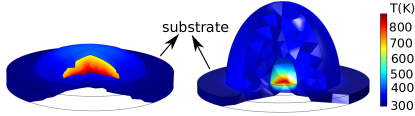
Figure S3: Temperature distribution $T(\mathbf{x})$ of the Ti (left) and Si₃N₄ (right) hemispheroid composites described in Fig. 1. Both structures rest on a SiO₂ substrate (thickness 0.3$\mu$m and radius $=1.5\times$ shell radius) whose bottom surface is in contact with a heat reservoir at 300 K. All other surfaces are exposed to vacuum and therefore satisfy adiabatic boundary conditions; material interfaces on the other hand are subject to thermal boundary resistance in accordance with operating condition (iii) and (ii) described in the text, for the left and right body, respectively.

Table 1: The thermal properties used in our COMSOL simulation

	k(W/m/K)	C(J/kg/K)
Ti	21.9	523
Si3N4	40	1100
GST	$\kappa(T)$ Lyeo et al. (2006)	208.3
SiO2	1.38	703

In order to solve the heat–conduction equation to obtain the steady-state temperature distribution $T(\mathbf{x})$, one must also specify the boundary conditions associated with vacuum–material interfaces, which we assume to be adiabatic ($\nabla T\cdot\mathbf{\hat{n}}=0$), corresponding to negligible conduction, convection, and radiative-heat dissipation through air. The substrate is chosen to be a 0.3$\leavevmode\nobreak\ \mu$m thick SiO₂ film in contact with a heat reservoir at 300 K through the bottom interface, leading to large heat dissipation away from the shell and hence large temperature localization in the GST with decreasing substrate thickness. We choose the substrate lateral (cylindrical) dimensions to be large enough to remove large thermal diffusion away from the GST. Figure S3 shows the temperature distribution of both Ti (left) and Si₃N₄ (right) structures under the operating condition (iii) and (ii), respectively, assuming the material conductivities and heat capacities given in Table I. As shown, the temperature in the substrate and shells is almost uniform and close to 300 K, thanks to the presence of boundary resistance between the heater and substrate (which bars heat from flowing into the substrate) along with the high thermal conductivities of Ti and Si₃N₄, which act to dissipate heat away from the GST.

References

- Greffet and Henkel (2007) J.-J. Greffet and C. Henkel, Contemporary Physics 48, 183 (2007).
- Masuda et al. (1988) K. Masuda, T. Takashima, and Y. Takayama, Remote Sensing of Environment 24, 313 (1988).
- Ilic and Soljačić (2014) O. Ilic and M. Soljačić, Nature materials 13, 920 (2014).
- Rinnerbauer et al. (2014) V. Rinnerbauer, A. Lenert, D. M. Bierman, Y. X. Yeng, W. R. Chan, R. D. Geil, J. J. Senkevich, J. D. Joannopoulos, E. N. Wang, M. Soljačić, et al., Advanced Energy Materials 4 (2014).
- Fan (2014) S. Fan, Nature nanotechnology 9, 92 (2014).
- Bermel et al. (2011) P. Bermel, M. Ghebrebrhan, M. Harradon, Y. X. Yeng, I. Celanovic, J. D. Joannopoulos, and M. Soljacic, Nanoscale research letters 6, 1 (2011).
- Florescu et al. (2007) M. Florescu, H. Lee, I. Puscasu, M. Pralle, L. Florescu, D. Z. Ting, and J. P. Dowling, Solar Energy Materials and Solar Cells 91, 1599 (2007).
- Cahill et al. (2003) D. G. Cahill, W. K. Ford, K. E. Goodson, G. D. Mahan, A. Majumdar, H. J. Maris, R. Merlin, and S. R. Phillpot, Journal of Applied Physics 93, 793 (2003).
- Cahill et al. (2014) D. G. Cahill, P. V. Braun, G. Chen, D. R. Clarke, S. Fan, K. E. Goodson, P. Keblinski, W. P. King, G. D. Mahan, A. Majumdar, et al., Applied Physics Reviews 1, 011305 (2014).
- De Zoysa et al. (2012) M. De Zoysa, T. Asano, K. Mochizuki, A. Oskooi, T. Inoue, and S. Noda, Nature Photonics 6, 535 (2012).
- Wang et al. (2014) W. Wang, C. Fu, and W. Tan, Journal of Quantitative Spectroscopy and Radiative Transfer 132, 36 (2014).
- Greffet et al. (2002) J.-J. Greffet, R. Carminati, K. Joulain, J.-P. Mulet, S. Mainguy, and Y. Chen, Nature 416, 61 (2002).
- Marquier et al. (2004) F. Marquier, K. Joulain, J.-P. Mulet, R. Carminati, J.-J. Greffet, and Y. Chen, Physical Review B 69, 155412 (2004).
- Joulain et al. (2005) K. Joulain, J.-P. Mulet, F. Marquier, R. Carminati, and J.-J. Greffet, Surf. Sci. Rep. 57, 59 (2005).
- Hesketh et al. (1988) P. J. Hesketh, J. N. Zemel, and B. Gebhart, Physical Review B 37, 10803 (1988).
- Narayanaswamy and Chen (2005) A. Narayanaswamy and G. Chen, Journal of Quantitative Spectroscopy and Radiative Transfer 93, 175 (2005).
- Marquier et al. (2015) F. Marquier, D. Costantini, A. Lefebvre, A.-L. Coutrot, I. Moldovan-Doyen, J.-P. Hugonin, S. Boutami, H. Benisty, and J.-J. Greffet, in SPIE OPTO (International Society for Optics and Photonics, 2015), pp. 937004–937004.
- Kleiner et al. (2012) V. Kleiner, N. Dahan, K. Frischwasser, and E. Hasman, in SPIE OPTO (International Society for Optics and Photonics, 2012), pp. 82700R–82700R.
- Ribaudo et al. (2013) T. Ribaudo, D. W. Peters, A. R. Ellis, P. S. Davids, and E. A. Shaner, Optics express 21, 6837 (2013).
- Kollyukh et al. (2003) O. Kollyukh, A. Liptuga, V. Morozhenko, and V. Pipa, Optics Communications 225, 349 (2003).
- Ben-Abdallah (2004) P. Ben-Abdallah, JOSA A 21, 1368 (2004).
- Drevillon et al. (2011) J. Drevillon, K. Joulain, P. Ben-Abdallah, and E. Nefzaoui, Journal of Applied Physics 109, 034315 (2011).
- Wang et al. (2011) L. Wang, S. Basu, and Z. Zhang, Journal of Heat Transfer 133, 072701 (2011).
- Lee et al. (2008) B. Lee, L. Wang, and Z. Zhang, Optics Express 16, 11328 (2008).
- Fu and Zhang (2009) C. Fu and Z. M. Zhang, Frontiers of Energy and Power Engineering in China 3, 11 (2009).
- Liu et al. (2011a) X. Liu, T. Tyler, T. Starr, A. F. Starr, N. M. Jokerst, and W. J. Padilla, Phys. Rev. Lett. 107, 045901 (2011a).
- Liu et al. (2011b) X. Liu, T. Tyler, T. Starr, A. F. Starr, N. M. Jokerst, and W. J. Padilla, Physical review letters 107, 045901 (2011b).
- Curto et al. (2010) A. G. Curto, G. Volpe, T. H. Taminiau, M. P. Kreuzer, R. Quidant, and N. F. van Hulst, Science 329, 930 (2010).
- Kosako et al. (2010) T. Kosako, Y. Kadoya, and H. F. Hofmann, Nature Photonics 4, 312 (2010).
- Teperik and Degiron (2011) T. Teperik and A. Degiron, Physical Review B 83, 245408 (2011).
- Thomas et al. (2004) M. Thomas, J.-J. Greffet, R. Carminati, and J. Arias-Gonzalez, Applied physics letters 85, 3863 (2004).
- Li et al. (2007) C. Li, G. W. Kattawar, Y. You, P. Zhai, and P. Yang, Journal of Quantitative Spectroscopy and Radiative Transfer 106, 257 (2007).
- Vandenbem et al. (2009) C. Vandenbem, L. Froufe-Pérez, and R. Carminati, Journal of Optics A: Pure and Applied Optics 11, 114007 (2009).
- Vandenbem et al. (2010) C. Vandenbem, D. Brayer, L. Froufe-Pérez, and R. Carminati, Physical Review B 81, 085444 (2010).
- Mohammadi et al. (2008) A. Mohammadi, V. Sandoghdar, and M. Agio, New Journal of Physics 10, 105015 (2008).
- Schuller et al. (2009) J. A. Schuller, T. Taubner, and M. L. Brongersma, Nature Photonics 3, 658 (2009).
- Novotny and Van Hulst (2011) L. Novotny and N. Van Hulst, Nature Photonics 5, 83 (2011).
- Balanis (2005) C. A. Balanis, Antenna theory: analysis and design, vol. 1 (John Wiley & Sons, 2005).
- Taminiau et al. (2007) T. H. Taminiau, R. J. Moerland, F. B. Segerink, L. Kuipers, and N. F. van Hulst, Nano letters 7, 28 (2007).
- Alavi Lavasani and Pakizeh (2012) S. Alavi Lavasani and T. Pakizeh, JOSA B 29, 1361 (2012).
- Shegai et al. (2011) T. Shegai, S. Chen, V. D. Miljković, G. Zengin, P. Johansson, and M. Käll, Nature communications 2, 481 (2011).
- Balandin (2011) A. A. Balandin, Nature materials 10, 569 (2011).
- Reifenberg et al. (2008) J. P. Reifenberg, D. L. Kencke, and K. E. Goodson, Electron Device Letters, IEEE 29, 1112 (2008).
- Marconnet et al. (2013) A. M. Marconnet, M. A. Panzer, and K. E. Goodson, Reviews of Modern Physics 85, 1295 (2013).
- Stevens et al. (2007) R. J. Stevens, L. V. Zhigilei, and P. M. Norris, International Journal of Heat and Mass Transfer 50, 3977 (2007).
- Merabia et al. (2009) S. Merabia, P. Keblinski, L. Joly, L. J. Lewis, and J.-L. Barrat, PRE 79, 021404 (2009).
- Islam et al. (2013) S. Islam, Z. Li, V. E. Dorgan, M.-H. Bae, and E. Pop, Electron Device Letters, IEEE 34, 166 (2013).
- Yeo et al. (2014) J. Yeo, G. Kim, S. Hong, J. Lee, J. Kwon, H. Lee, H. Park, W. Manoroktul, M.-T. Lee, B. J. Lee, et al., Small 10, 5015 (2014).
- King et al. (2013) W. P. King, B. Bhatia, J. R. Felts, H. J. Kim, B. Kwon, B. Lee, S. Somnath, and M. Rosenberger, Annual Review of Heat Transfer 16 (2013).
- Petit-Watelot et al. (2012) S. Petit-Watelot, R. M. Otxoa, M. Manfrini, W. Van Roy, L. Lagae, J.-V. Kim, and T. Devolder, Physical review letters 109, 267205 (2012).
- Dombrovsky (2000) L. A. Dombrovsky, International Journal of Heat and Mass Transfer 43, 1661 (2000).
- Luo et al. (2004) C. Luo, A. Narayanaswamy, G. Ghen, and J. D. Joannopoulos, Phys. Rev. Lett. 93, 213905 (2004).
- Polimeridis et al. (2015) A. G. Polimeridis, M. Reid, W. Jin, S. G. Johnson, J. K. White, and A. W. Rodriguezz, arXiv preprint arXiv:1505.05026 (2015).
- Polimeridis et al. (2014) A. Polimeridis, J. Villena, L. Daniel, and J. White, Journal of Computational Physics 269, 280 (2014).
- Landau et al. (1960) L. D. Landau, E. M. Lifshitz, and L. P. Pitaevskiĭ, Statistical Physics Part 2, vol. 9 (Pergamon, Oxford, 1960).
- Rodriguez et al. (2013) A. W. Rodriguez, M. H. Reid, and S. G. Johnson, Physical Review B 88, 054305 (2013).
- Johnson (2011) S. G. Johnson, in Casimir Physics, edited by D. A. R. Dalvit, P. Milonni, D. Roberts, and F. d. Rosa (Springer–Verlag, 2011), vol. 836 of Lecture Notes in Physics, chap. 6, pp. 175–218.
- Xiong et al. (2009) F. Xiong, A. Liao, and E. Pop, Applied Physics Letters 95, 243103 (2009).
- Liang et al. (2012) J. Liang, R. G. D. Jeyasingh, H.-Y. Chen, and H. Wong, Electron Devices, IEEE Transactions on 59, 1155 (2012).
- Note (1) Note1, note that at these temperatures convective and radiative effects are negligible compared to conductive transfer, allowing us to consider the radiation and conduction problems separately.
- Lyeo et al. (2006) H.-K. Lyeo, D. G. Cahill, B.-S. Lee, J. R. Abelson, M.-H. Kwon, K.-B. Kim, S. G. Bishop, and B.-k. Cheong, Applied Physics Letters 89, 151904 (2006).
- Tsafack et al. (2011) T. Tsafack, E. Piccinini, B.-S. Lee, E. Pop, and M. Rudan, Journal of Applied Physics 110, 063716 (2011).
- Shportko et al. (2008) K. Shportko, S. Kremers, M. Woda, D. Lencer, J. Robertson, and M. Wuttig, Nature materials 7, 653 (2008).
- Li et al. (2008) X. Z. Li, J. K. Choi, Y. S. Byun, S. Y. Kim, K. S. Sim, and S. K. Kim, Japanese Journal of Applied Physics 47, 5477 (2008).
- Mash and Motulevich (1973) I. Mash and G. Motulevich, SOVIET PHYSICS JETP 36 (1973).
- Kischkat et al. (2012) J. Kischkat, S. Peters, B. Gruska, M. Semtsiv, M. Chashnikova, M. Klinkmüller, O. Fedosenko, S. Machulik, A. Aleksandrova, G. Monastyrskyi, et al., Applied optics 51, 6789 (2012).
- Bohren and Huffman (2008) C. F. Bohren and D. R. Huffman, Absorption and scattering of light by small particles (John Wiley & Sons, 2008).
- Yu et al. (2013) Z. Yu, N. P. Sergeant, T. Skauli, G. Zhang, H. Wang, and S. Fan, Nature communications 4, 1730 (2013).
- Weinstein (1960) M. Weinstein, American Journal of Physics 28, 123 (1960).
- Fischer and Fellmuth (2005) J. Fischer and B. Fellmuth, Reports on progress in physics 68, 1043 (2005).
- Banaei and Abouraddy (2013) E.-H. Banaei and A. F. Abouraddy, Progress in Photovoltaics: Research and Applications (2013).
- Le Ru and Etchegoin (2008) E. Le Ru and P. Etchegoin, Principles of Surface-Enhanced Raman Spectroscopy and related plasmonic effects (Elsevier Science, 2008).
- Rudé et al. (2013) M. Rudé, J. Pello, R. E. Simpson, J. Osmond, G. Roelkens, J. J. van der Tol, and V. Pruneri, Applied Physics Letters 103, 141119 (2013).
- Kim et al. (2012) J. Kim, G. V. Naik, N. K. Emani, and A. Boltasseva, arXiv preprint arXiv:1211.5988 (2012).
- Shahil and Balandin (2012) K. M. Shahil and A. A. Balandin, Solid State Communications 152, 1331 (2012).