OCU-PHYS 427

July, 2015

Developments of theory of effective prepotential

from extended Seiberg-Witten system
and matrix models

H. Itoyama^a,b and R. Yoshioka^b

^a Department of Mathematics and Physics, Graduate School of Science
Osaka City University

^b Osaka City University Advanced Mathematical Institute (OCAMI)

3-3-138, Sugimoto, Sumiyoshi-ku, Osaka, 558-8585, Japan

Abstract

This is a semi-pedagogical review of a medium size on the exact determination of and the role played by the low energy effective prepotential ${\cal F}$ in QFT with (broken) extended supersymmetry, which began with the work of Seiberg and Witten in 1994. While paying an attention to an overall view of this subject lasting long over the two decades, we probe several corners marked in the three major stages of the developments, emphasizing uses of the deformation theory on the attendant Riemann surface as well as its close relation to matrix models. Examples picked here in different contexts tell us that the effective prepotential is to be identified as the suitably defined free energy $F$ of a matrix model: ${\cal F}=F$.

To be submitted to PTEP as an invited review article and based in part on the talk delivered by one of the authors (H.I.) in the workshop held at Shizuoka University, Shizuoka, Japan, on December 5, 2014.

1 Introduction

The notion of effective action plays a vital role in the modern treatment of quantum field theory. (See, for instance, [1, 2].) In this review article, we deal with a special class of low energy effective actions that are controlled by (broken) extended rigid supersymmetry in four spacetime dimensions and permit exact determination exploiting integrals on a Riemann surface in question. A main object in such study is the low energy effective prepotential to be denoted by $\mathcal{F}$ generically in this paper, which has proven to be central not only in the original case of unbroken ${\cal N}=2$ supersymmetry initiated by the work of Seiberg-Witten [3, 4] but also in the case where this symmetry is broken by the vacuum or by the superpotential. The review will be presented basically in a chronological order, following the three major stages of the developments that took place during the periods $1994\sim$, $2002\sim$ and $2009\sim$. Each of the three subsequent sections will explain pieces of work done in its respective period.

An emphasis will be put on the deformation theory of the effective prepotential on the Riemann surface as an extension of the Seiberg-Witten system consisting of the curve, the meromorphic differential and the period as well as its close relation to matrix models.

We conclude from the examples taken here in the different contexts that the effective prepotential is in fact identified as the suitably defined free energy $F$ of a matrix model: ${\cal F}=F$. While this is hardly a surprising conclusion from the point of view of mathematics of integrable systems and soliton hierarchies, the number of examples in QFT where this is explicitly materialized is not large enough. This note may serve to improve the situation.

In the next section, after presenting the curve for $\mathcal{N}=2$, $SU(N)$ pure super Yang-Mills theory as a spectral curve of the periodic Toda chain, we discuss the deformation of the effective prepotential by placing higher order poles to the original meromorphic differential. We give a derivation of the formula which the meromorphic differential extended this way obeys.

In section three, we discuss the degeneration phenomenon of the Riemann surface necessary to describe the $\mathcal{N}=1$ vacua that lie in the confining phase and introduce the prepotential having gluino condensates as variables. We apply the formalism in section 2 here, and describe the situation by the use of mixed second derivatives. After discussing the emergence of the matrix model curve and giving sample calculation, we finish the section with the case of spontaneously broken $\mathcal{N}=2$ supersymmetry in order to illustrate the role played by the two distinct singlet operators one of which is the QFT counterpart of the matrix model resolvent.

In section four, we go back to the situation of $\mathcal{N}=2$ and discuss the developments associated with the AGT relation and the upgraded treatment of the all-genus instanton partition function and therefore the deformation of the Seiberg-Witten curve to its noncommutative counterpart. A finite $N$ and $\beta$-deformed matrix model with filling fractions specified emerge as an integral representation of the conformal/W block and we discuss the direct evaluation of its $q$-expansion as the Selberg integral. We finish the section with mentioning some of the more recent developments.

Please note that the model or theory hops from one to the other as the sections proceed and that each section has its open ending, indicating calls for further developments of this long lasting subject.

2 effective prepotential from extended Seiberg-Witten system

We will not give here an account of the construction of the curve itself [3, 4, 5, 6, 7, 8, 9], (for a recent review, for instance, [10]) nor its connection to classical integrable system [11, 12, 13, 14, 15, 16, 17, 18, 19, 20, 21, 22, 23, 24, 25, 26]. Also omitted is the discussion associated with the WDVV equation, for which we direct the readers to [27, 28, 29] as well as references contained in [30, 31].

2.1 curves, periods and meromorphic differentials

The list of papers which discuss subjects closely related to that of this subsection include [3, 4, 5, 6, 14, 7, 8, 32, 15, 16, 9, 17, 18, 19, 20, 21, 22, 23, 24, 25, 33, 34, 35, 36, 37, 38, 39, 40, 41, 42, 43, 44, 45, 46, 47, 48, 49, 50, 51, 52, 53, 54, 55, 31, 56, 57, 10].

Let us recall the most typical situation and consider the low energy effective action (LEEA) for $\mathcal{N}=2$, $SU(N)$ pure super Yang-Mills theory. The symmetry of LEEA at the scale much smaller than that of the W boson mass is $U(1)^{N-1}$. The relevant curve is a hyperelliptic Riemann surface of genus $N-1$ described as

$$Y^{2} =P_{N}^{2}(x)-4\Lambda^{2N},$$ (2.1)

$${\rm where}$$

$$P_{N}(x) =\langle\det(x{\bf 1}-\Phi)\rangle\equiv\prod_{i=1}^{N}(x-{p_{i}})=x^{N}-\sum_{k=2}^{N}{u_{k}}x^{N-k}$$

$$=\sum_{k=0}^{N}s_{k}(h_{\ell})x^{N-k}.$$ (2.2)

Here,

$${h_{\ell}}=\frac{1}{\ell}\langle{\rm tr}\Phi^{\ell}\rangle=\frac{1}{\ell}\sum_{i=1}^{N}{p_{i}^{\ell}},~{}~{}~{}~{}~{}~{}\ell=2,3,\cdots,N,$$ (2.3)

and $s_{k}(h_{\ell})$ are the appropriate Schur polynomials. Introducing the spectral parameter $z$, we write the curve as that of the periodic Toda chain:

$$P_{N}(x) =z+\frac{{\Lambda^{2N}}}{z},$$ (2.4)

$$Y =z-\frac{{\Lambda^{2N}}}{z}.$$ (2.5)

Figure 1:

The distinguished meromorphic differential for the construction of the effective prepotential is given by

$$\mathrm{d}\hat{S}_{\rm SW}=x\mathrm{d}\log z=x{t(x)}\mathrm{d}x,~{}~{}~{}{t(x)}=\frac{P^{\prime}_{N}}{\sqrt{P_{N}^{2}-4\Lambda^{2}}}.$$

The characteristic feature of this is the existence of double poles at $\infty_{\pm}$. Later in this section, we interpret this to be the case where only $T_{1}$ has been turned on.

The defining property is that the moduli derivatives are holomorphic:

$$\left.\frac{\partial}{\partial u_{k}}\mathrm{d}\hat{S}_{\rm SW}\right|_{{z},\Lambda} =\frac{x^{N-k}}{Y}\mathrm{d}x,$$ (2.6)

or

$$\left.\frac{\partial}{\partial u_{k}}\mathrm{d}\hat{S}_{\rm SW}\right|_{{x},\Lambda} =\frac{x^{N-k}}{Y}\mathrm{d}x-\mathrm{d}\left(\frac{x^{N-k+1}}{Y}\right).$$ (2.7)

The prepotential $\mathcal{F}_{\rm SW}$ is introduced implicitly by the A cycle and B cycle integrations on the Riemann surface:

$$a_{i}=\oint_{A_{i}}\mathrm{d}\hat{S}_{\rm SW},~{}~{}~{}~{}~{}\frac{\partial\mathcal{F}_{\rm SW}}{\partial a_{i}}(=a^{D}_{i})=\oint_{B_{i}}\mathrm{d}\hat{S}_{\rm SW}.$$ (2.8)

While $u_{k}$ possess invariant meaning both in the moduli space of the Riemann surface and in the integrable system, it is these constant background fields or Coulomb moduli $a_{i}$, $a^{D}_{i}=\frac{\partial\mathcal{F}_{\rm SW}}{\partial a_{i}}$ which are directly related to the observables through the BPS formula. The moduli derivatives are coordinate dependent as we see in eqs. (2.6) and (2.7). The final expression for $\mathcal{F}_{\rm SW}$ is going to be coordinate independent. This is supported by the pieces of evidence we present here that the effective prepotential is identified as the free energy of a matrix model.

2.2 Whitham deformation of the prepotential and the appearance of “thermodynamic” relation

The list of papers which discuss subjects closely related to that of this subsection include [58, 59, 60, 24, 61, 62, 63, 64, 65, 66, 67, 68, 69, 31, 57].

We would now like to review the deformation of the effective prepotential above which we have denoted by $\mathcal{F}_{\rm SW}$. The basic idea of this extended theory of effective prepotential often referred to as Whitham deformation is to deform both moduli of the Riemann surface and the meromorphic differential above consistently without losing the defining properties:

$$\mathrm{d}\hat{S}_{\rm SW}\to{\mathrm{d}\hat{S}};~{}~{}~{}~{}~{}\frac{\partial}{\partial h_{k}}{\mathrm{d}\hat{S}}|_{{*},\Lambda}=\text{holomorphic}.$$ (2.9)

We have adopted the choice that $z$ is fixed when the moduli derivatives are taken. We carry out the deformation by adding higher order poles to the original meromorphic differential containing the double poles. Let us denote the local coordinates in their neighborhood generically by $\xi$ and

$${\xi=z^{\mp\frac{1}{N}}~{}~{}{\rm or}~{}~{}x^{-1}}\;.$$ (2.10)

In order to describe the deformation, let us introduce a set of meromorphic differentials $\mathrm{d}\Omega_{\ell}$ that satisfy

$$\mathrm{d}\Omega_{\ell}=\xi^{-\ell-1}\mathrm{d}\xi+\text{non-singular \; part}~{}~{}~{}~{}\ell=1.2,3,\cdots\;\;.$$ (2.11)

We are still left with the ambiguities that any linear combination of the canonical holomorphic differentials $\mathrm{d}\omega_{i}$ can be added to the right hand side. In order to remove these, let us require a set of conditions

$$\oint_{{A_{i}}}\mathrm{d}\Omega_{\ell}=0\;\;.$$ (2.12)

The ones which are not subject to the conditions eq.(2.12) are denoted by $\mathrm{d}\widehat{\Omega}_{\ell}$.

Let us first state the formula

$${\mathrm{d}\hat{S}=\sum_{i=1}^{g}{a^{i}}\mathrm{d}\omega_{i}+\sum_{\ell\geq 1}{T_{\ell}}\mathrm{d}\Omega_{\ell}}\;\;$$ (2.13)

and outline its derivation below. As before, $a^{i}$ are defined to be the local coordinates in the moduli space

$${a^{i}}\equiv\oint_{A_{i}}\mathrm{d}\hat{S}\;\;,$$ (2.14)

while $T_{\ell}$, referred to as time variables or T moduli, are given by

$${T_{\ell}}=\underset{\xi=0}{\rm res}\xi^{\ell}\mathrm{d}\hat{S}\;\;,$$ (2.15)

once eq.(2.13) is established. One then regards $a^{i}$ and $T_{\ell}$ as independent, taking $h_{k}$ dependent: ${h_{k}=h_{k}}({a^{i},T_{\ell}})$. The (extended) effective prepotential ${\mathcal{F}}({a^{i},T_{\ell}})$ is introduced via

$$\frac{\partial{\mathcal{F}}}{\partial{a^{i}}}=\oint_{B^{i}}\mathrm{d}\hat{S},~{}~{}~{}\frac{\partial{\mathcal{F}}}{\partial{T_{\ell}}}=\frac{1}{2\pi\mathrm{i}\ell}{\rm res}\xi^{-\ell}\mathrm{d}\hat{S}\equiv{\mathcal{H}_{\ell+1}}{(h_{k})}\;.$$ (2.16)

The derivation of eq.(2.13) begins with the introduction of the time variables $T_{\ell}$ via a solution $\mathrm{d}\hat{S}(T_{\ell}|h)$ to eq.(2.9),

$$\text{namely,}~{}~{}~{}~{}\frac{\partial\mathrm{d}\hat{S}}{\partial T_{\ell}}=\mathrm{d}\Omega_{\ell}\;\;,~{}~{}~{}~{}~{}\text{and~{}~{} hence}~{}~{}~{}~{}~{}~{}~{}~{}\frac{\partial a_{i}}{\partial T_{\ell}}=0\;.$$ (2.17)

In terms of our intermediate bases $\mathrm{d}\widehat{\Omega}_{\ell}$, eq.(2.9) reads

$$\frac{\partial}{\partial h_{k}}\mathrm{d}\hat{\Omega}_{\ell}=\sum_{i=1}^{g}\sigma_{ki}^{(\ell)}\mathrm{d}\omega_{i},$$ (2.18)

while $$\mathrm{d}\widehat{\Omega}_{\ell}=\mathrm{d}{\Omega}_{\ell}+\sum_{i=1}^{g}c_{i}^{(\ell)}\mathrm{d}\omega_{i}\;\;,$$ (2.19)

as the difference between $\mathrm{d}\hat{\Omega}_{\ell}$ and $\mathrm{d}{\Omega}_{\ell}$ can be spanned by the holomorphic differentials. Expand the solutions as

$$\mathrm{d}\hat{S}=\sum_{m}\beta_{m}(T)\mathrm{d}\widehat{\Omega}_{m}(h)\;\;,$$ (2.20)

hence $$\frac{\partial\mathrm{d}\hat{S}}{\partial T_{n}}=\sum_{m}\left(\frac{\partial\beta_{m}}{\partial T_{n}}\mathrm{d}\widehat{\Omega}_{m}+\beta_{m}\sum_{k}\frac{\partial h_{k}}{\partial T_{n}}\sum_{i=1}^{g}\sigma_{ki}^{(m)}\mathrm{d}\omega_{i}\right).$$ (2.21)

Exploiting eq.(2.17), eq.(2.19) and eq.(2.21), we obtain

$$\frac{\partial\beta_{m}}{\partial T_{n}}=\delta_{m,n}~{}~{}~{}~{}~{}{\rm i.e.}~{}~{}\beta_{m}(T)=T_{m}$$ (2.22)

as well as $$\sum_{k}\frac{\partial h_{k}}{\partial T_{n}}\left(\sum_{m}T_{m}\sigma_{ki}^{(m)}\right)=-c_{i}^{(n)}.$$ (2.23)

Substituting eq.(2.22) and eq.(2.19) into eq.(2.20), we obtain

$$\mathrm{d}\hat{S}=\sum_{m}T_{m}\mathrm{d}\Omega_{m}+\sum_{m}T_{m}\sum_{i}c_{i}^{(m)}\mathrm{d}\omega_{i},$$ (2.24)

whose integrations over the $A_{i}$ cycles yield

$$a_{i}=\sum_{m}T_{m}c_{i}^{(m)}.$$ (2.25)

This shows eq.(2.13).

2.3 connection with the planar free energy of matrix models

Already at this stage of the developments, a keen connection of the extended Seiberg-Witten system with the construction of matrix models in general, or more specifically, the similarity of the effective prepotentials with the (planar) free energy of matrix models was visible. In fact, starting from the homogeneity of the moduli and the prepotential, it is possible to derive an integral expression for ${\mathcal{F}}$ which resembles that of matrix model planar free energy in terms of the density one-form on the eigenvalue coordinate. See, eq. (4.12) of [24]. Also [14, 16, 18].

One of the goals of the present review is to put together subsequent several developments that took place and have made this phenomenon more prominent. These are presented in the next two sections.

3 Gluino condensate prepotential

One major use of the deformation theory of the effective prepotential presented above took place in the context of gluino condensate prepotential built on various $\mathcal{N}=1$ vacua in contrast to ${\mathcal{F}}_{\rm SW}$ and its extension in section 2. We first consider the case in which the breaking to $\mathcal{N}=1$ from $\mathcal{N}=2$ supersymmetry is caused by the superpotential in the action. Later we will contrast this with the case in which $\mathcal{N}=2$ is broken spontaneously to $\mathcal{N}=1$ at the tree level [70, 71, 72, 73, 74].

3.1 degeneration phenomenon and mixed second derivatives

The list of papers which discuss subjects closely related to that of this subsection include [76, 75, 77, 78, 79, 80, 81, 82, 83, 84, 85, 86, 87, 88, 89, 90, 91, 92, 93, 94, 95, 30, 96, 97, 98, 99, 100, 101, 102, 103, 104, 105, 106].

Let’s fix an action to work with: it is a $U(N)$ gauge theory consisting of adjoint vector superfields and chiral superfields with canonical kinematic factors and the superpotential turned on in the $\mathcal{N}=2$ action drives the system to its $\mathcal{N}=1$ vacua.

As a phenomenon occurring on a Riemann surface, we consider the situation where a degeneration takes place and some of the cycles coalesce to form a new set of cycles. As for the description of the low energy effective action (LEEA), some of the original Coulomb moduli disappear and the product of these $U(1)$ s gets replaced by non-Abelian gauge symmetry ${\displaystyle{\prod_{i=1}^{n}SU(N_{i})}}$. We tabulate these pictures below.

	$\mathcal{N}=2$		$\mathcal{N}=1$
	$U(N)$ pure SYM	$\xrightarrow[\begin{subarray}{c}{\rm deformed}\\ \text{by superpotential}\end{subarray}]{}$	$\displaystyle{\prod_{i=1}^{n}U(N_{i})}$
	$\displaystyle{g_{n+1}\int\mathrm{d}^{2}\theta{\rm tr}W_{n+1}(\Phi)}$     such that $\displaystyle{W_{n+1}^{\prime}(x)=\prod_{i=1}^{n}(x-\alpha_{i})}$
LEEA	$\underset{\lower 8.61108pt\vbox to-2.0pt{\hbox{\small{\rm Coulomb}}}}{\displaystyle{U(1)^{N-1}\times U(1)}}$	$\longrightarrow$	$\underset{\lower 8.61108pt\vbox to-2.0pt{\hbox{\small{\rm Coulomb}}}}{\displaystyle{U(1)^{n-1}\times U(1)}}\times\underset{\lower 0.0pt\vbox to0.0pt{\hbox{\small{\rm confining}}}}{\displaystyle{\prod_{i=1}^{n}SU(N_{i})}}$
RS		$\xrightarrow[\rm degeneration]{}$

The $\mathcal{N}=1$ vacua are labelled by the set of order parameters representing gluino condensates:

$$S_{i}\propto{\rm Tr}_{SU(N_{i})}W^{\alpha}W_{\alpha},~{}~{}~{}~{}~{}i=1,\cdots,n.$$ (3.1)

The proportionality constant will be fixed in subsequent subsections.

We now review, following the observation made in [105] that the condition for a curve to degenerate or factorize is given by that the kernel of the matrix made of the mixed second derivatives of the deformed prepotential be nontrivial.

Continuing with the general discussion of subsection 2.2, let us first note that we obtain two different expressions for the mixed second derivatives from eq.(2.16):

$$\frac{\partial^{2}\mathcal{F}}{\partial a^{i}\partial T_{\ell}}=\oint_{B_{i}}\mathrm{d}\Omega_{\ell}=\frac{1}{2\pi\mathrm{i}\ell}{\rm res}\xi^{-\ell}\mathrm{d}\omega_{i},~{}~{}~{}~{}~{}i=1,\cdots,N-1,~{}~{}~{}~{}\ell:\text{ positive integers}$$ (3.2)

We impose the condition

$${\rm ker}\frac{\partial^{2}\mathcal{F}}{\partial a^{i}\partial T_{\ell}}\neq 0,~{}~{}~{}{\rm or}~{}~{}~{}{\rm rank}\frac{\partial^{2}\mathcal{F}}{\partial a^{i}\partial T_{\ell}}\leq N-2.$$ (3.3)

Eq.(3.3) has following straightforward implications:
i) there exists a nonvanishing column vector $\begin{pmatrix}c^{1},~{}c^{2},~{}\cdots~{}c^{N-1},~{}\cdots\end{pmatrix}^{t}$ such that

$$0=\sum_{\ell}\frac{\partial^{2}\mathcal{F}}{\partial a^{i}\partial T_{\ell}}c^{\ell}\underset{eq.\eqref{(1)}}{=}\sum_{\ell}\oint_{B_{i}}\mathrm{d}\Omega_{\ell}c^{\ell}\underset{eq.\eqref{higherorderpole}}{=}\frac{1}{2\pi\mathrm{i}}\underset{\xi=0}{\rm res}\left(\sum_{\ell}\frac{c^{\ell}}{\ell}\xi^{-\ell}\right)_{+}\mathrm{d}\omega_{i}\;\;.$$ (3.4)

Here, we have exploited eq. (2.17) in the second equality and eq. (2.10) in the third equality. The former equality implies that $\displaystyle{\mathrm{d}\widetilde{\Omega}\equiv\sum_{\ell}c^{\ell}\mathrm{d}\Omega_{\ell}}$ has vanishing periods over all $A_{i}$ & $B^{i}$ cycles.Then one can integrate this form along any path ending with a point $z$ to define a function holomorphic except at punctures. As for the order of the poles at the punctures, it is generically arbitrary according to the construction. But this is contradictory to the Weierstrass gap theorem derived from the Riemann-Roch theorem. To avoid a contradiction, we must have a degeneration.

ii) there exists a nonvanishing row vector $\begin{pmatrix}\widetilde{c}_{1},\widetilde{c}_{2},\cdots,\widetilde{c}_{N-1}\end{pmatrix}$ such that

$$0=\sum_{i=1}^{N-1}\widetilde{c}_{i}\frac{\partial^{2}\mathcal{F}}{\partial a^{i}\partial T_{\ell}}=\sum_{i}\widetilde{c}_{i}\frac{\partial\mathcal{H}_{\ell+1}}{\partial a^{i}}$$ (3.7)

in accordance with the second formula of eq. (2.16). Eq. (3.7) follows from

$$\sum_{i}\widetilde{c}_{i}\frac{\partial h_{\ell+1}}{\partial a^{i}}=0\;,$$ (3.8)

which is regarded as the statement of the vanishing discriminant. The moduli depend actually on less than $N-1$ arguments.

3.2 emergence of the matrix model curve

The list of papers which discuss subjects closely related to that of this subsection include [107, 108, 109, 110, 111, 112, 113, 114, 115, 116, 117, 118, 119, 120, 121, 30, 100, 122, 123, 105].

Once we are convinced of the degeneration of the surface, we can proceed further by factorizing the original curve, which, in the current example, is the hyperelliptic one.

Let $n-1$ be the number of genus after the degeneration. Following [88, 89], we state

$$\left(\begin{array}[]{l}\displaystyle{Y^{2}=H_{N-1}(x)^{2}F_{2n}(x)},\\ \\ P_{N}^{\prime}(x)=H_{N-n}(x)R_{n-1}(x)\;.\end{array}\right.$$ (3.9)

Finally let us examine the last equality of eq.(3.4). Let

$$\sum_{\ell=1}^{N-1}\frac{c_{\ell}}{\ell}\left(\xi^{-\ell}\right)_{+}\equiv{W^{\prime}_{k+1}(x)}{\equiv\prod_{j=1}^{k}(x-\alpha_{j})}.\\$$ (3.10)

and $\frac{x^{j-1}}{\sqrt{F_{2n}}}$ serve as bases of the holomorphic differentials of the reduced Riemann surface. Actually, only the $j=1\sim n-1$ differentials are holomorphic and the $j=n$ one has been added through the blow-up process, which physically implies that the overall $U(1)$ fails to decouple. We obtain

$$0=\underset{x=\infty}{\rm res}\left(W^{\prime}_{k+1}(x)\frac{x^{j-1}}{\sqrt{F_{2n}}}\right),$$ (3.11)

$${\rm and~{}therefore~{}~{}~{}}\frac{W^{\prime}_{k+1}}{\sqrt{F_{2n}}}=Q_{k-n}(x)+\sum_{\ell>n}\frac{\beta_{\ell}}{x^{\ell}}.$$ (3.12)

$${\rm We~{}obtain~{}~{}~{}}y^{2}\equiv F_{2n}Q_{k-n}^{2}=W^{\prime}_{k+1}+f_{k-1}.$$ (3.13)

Here, $f_{k-1}$ is a polynomial of degree $k-1$. This is the curve appearing in the $k$-cut solution of the matrix model.

We still need to see that $W_{k+1}(x)$ introduced above is in fact a tree level superpotential. This is easily done by taking the classical limit $\Lambda=0$:

$$Y=z=\prod_{\ell=1}^{N}(x-p_{\ell}).$$ (3.14)

The original Seiberg-Witten differential becomes

$$\mathrm{d}\hat{S}_{\rm SW}^{\rm(class)} =x\sum_{i=1}^{N}\frac{1}{x-p_{i}}\mathrm{d}x\;,$$ (3.15)

$${\rm which~{}is~{}equal~{}to~{}~{}~{}} =\sum_{i=1}^{N}p_{i}\mathrm{d}\omega_{i}+N\mathrm{d}x.$$ (3.16)

Here, we have used that the canonical holomorphic differential becomes

$$\mathrm{d}\omega_{i}^{\rm(class)}=\frac{\mathrm{d}x}{x-p_{i}}\;\;$$ (3.17)

in this limit. The period integrals over the $A_{i}$ cycles just pick up the residues at the poles $p_{i}$:

$${a_{i}^{\rm(class)}}=p_{i}.$$ (3.18)

The degeneration in this limit is described as

$$z=\prod_{j=1}^{n}(x-\beta_{j})^{N_{j}},~{}~{}\sum_{j=1}^{n}N_{j}=N\;.$$ (3.19)

In fact, the $N_{j}$ poles coalesce at $\beta_{j},~{}j=1,\cdots,n\;$ and the canonical holomorphic differentials on the degenerate curve are

$$\mathrm{d}\omega_{j}^{\rm(class,red)}=\frac{\mathrm{d}x}{x-\beta_{j}}\;\;.$$ (3.20)

The condition eq. (3.11) becomes

$$0=\underset{x=0}{\rm res}\left(W^{\prime}_{k+1}(x)\mathrm{d}\omega_{j}^{\rm(class,red)}\right),~{}~{}~{}~{}~{}j=1,\cdots,n,\;\;\;,$$ (3.21)

which tells us that ${\beta_{j}}$ must coincide with one of the roots ${\alpha_{j}}$ of $W^{\prime}_{k+1}$. The vev’s of the adjoint scalar fields are thus constrained to the extrema of $W_{k+1}$.

Let us set $k=n$ for simplicity. We have the reduced curve of $g=n-1$:

$$y^{2}=W^{\prime}_{n+1}(x;\alpha_{j})^{2}+f_{n-1}(x).$$ (3.22)

and let us denote the coefficients of the polynomial $f_{k-1}$ by $b_{\ell}(\alpha_{j})$, temporarily forgetting the $\alpha_{j}$ dependence. We also mention here that the full set of parameters (moduli) of the model realized by the curve eq. (3.22) is $2n$ dimensional and can be represented by the cut lengths and cut positions:

$${\rm dim(moduli)}=2n\approx\text{cut lengths}+\text{cut positions}.$$ (3.23)

Figure 2:

3.3 practical calculation

The list of papers which discuss subjects closely related to that of this subsection include [124, 125, 126, 127, 128, 97, 100, 129, 130, 131, 132, 133].

Let us now proceed to discuss the use of this machinery in calculation. As the condensates $S_{i}$ are quantum mechanical in nature, one can develop loop expansion using these, including the Veneziano-Yankielowicz term which contains the logarithmic singularity [77]. The first question to be raised is what the distinguished meromorphic differential is to be used for such calculation. It must be ”almost” holomorphic after the $b_{\ell}$ derivatives are taken. Recall that the bases of the ”holomorphic” differentials are taken as $\frac{x^{j-1}}{y},~{}j=1,\cdots,n-1,n$. Rather obviously, such differential is found as

$$\mathrm{d}\hat{S}_{\rm mat}=y(x)\mathrm{d}x,~{}~{}~{}~{}~{}~{}{\rm with}~{}~{}~{}~{}~{}~{}~{}~{}~{}~{}~{}~{}~{}T_{2},\cdots,T_{n},~{}T_{n+1}~{}~{}~{}~{}~{}~{}~{}~{}{\rm turned~{}~{}on}.$$ (3.24)

As before, the effective prepotential is introduced through the period integrals

$$\left({\begin{array}[]{llc}&~{}~{}~{}~{}~{}\displaystyle{{S_{i}}=\oint_{{A_{i}}}\mathrm{d}\hat{S}_{\rm mat}~{}~{}i=1,\cdots,n},{}{}{}{}{}{}{}{}{}{}&\\ {\rm and}&&\\ &~{}~{}~{}~{}~{}\displaystyle{\frac{\partial{\mathcal{F}}}{\partial{S_{i}}}}=2\int_{i~{}{\rm edge}}^{\rm cutoff}{\mathrm{d}\hat{S}_{\rm mat}}\;.&\end{array}}\right.$$ (3.25)

We have, however, no reason to set

$${S\equiv\sum_{i=1}^{n}S_{i}}=\int_{\prod_{i=1}^{n}~\!\!\!\!{}^{\cup}A_{i}}\mathrm{d}\hat{S}_{\rm mat}$$ (3.26)

equal to zero. This tells us the presence of the cutoff at the infinities of the surface.

The expansion of $\mathcal{F}$ in $S_{i}$ was done in [97], exploiting eq. (3.25) and the small cut expansion as an intermediate step originally. This provided the answer given below for $\mathcal{F}$ to the cubic order in $S_{i}$ (eq. (3.34) - (3.38)). Yet, there exists a simpler procedure, namely, a calculus from $T$ moduli thanks to the machinery discussed in the present review. The $T$ moduli are easily identified as

$${T_{m+1}}=\underset{\infty}{\rm res}~{}x^{-m-1}\mathrm{d}\hat{S}_{\rm mat}=gu_{m},~{}~{}~{}~{}~{}u_{m}=(-)^{n-m}e_{n-m}^{(\alpha)},$$ (3.27)

where

$$e_{m}(\alpha)=\sum_{i_{1}<\cdots<i_{m}}\alpha_{i_{1}}\cdots\alpha_{i_{m}}\;.$$ (3.28)

The dependence of the prepotential on the $T$ moduli is determined by the equations

$${{{\frac{1}{g}\frac{\partial\mathcal{F}}{\partial u_{\ell}}={\frac{\partial\mathcal{F}}{\partial T_{\ell+1}}}=\frac{1}{\ell+1}\underset{\infty}{\rm res}(x^{\ell+1}-\Lambda^{\ell+1})\mathrm{d}\hat{S}_{\rm mat}}}}.$$ (3.29)

Here $\Lambda^{\ell+1}$ is the term introduced in [100] in order to match with the computation done earlier. In order to carry out this task, we introduce intermediate expansion variables $\tilde{S}_{i}$ and parameterize the matrix model curve eq. (3.22) by

$$f_{n-1}(x)=\sum_{i=1}^{n}{\tilde{S}_{i}}\prod_{j(\neq i)}^{n}(x-\alpha_{j})=W^{\prime}_{n+1}(x)\sum_{i=1}^{n}\frac{{\tilde{S}_{i}}}{x-\alpha_{i}}.$$ (3.30)

The differential $\mathrm{d}\hat{S}_{\rm mat}$ of eq. (3.24) has a straightforward expansion in $\tilde{S}_{i}$. Therefore, $A_{i}$ cycle integrations followed by the inversion provide an expansion of $\tilde{S}_{i}$ in $S_{j}$

$$\tilde{S}_{i}=S_{i}+\frac{1}{2g}\sum_{j,k}\frac{1}{\alpha_{ij}\alpha_{ik}\Delta_{i}}S_{j}S_{k}+\cdots\;\;.$$ (3.31)

Here, we have introduced $\alpha_{ij}=\alpha_{i}-\alpha_{j}$, and $\displaystyle{\Delta_{i}=\prod_{j\neq i}\alpha_{ij}}$. Another useful machinery is the $T_{m}$ moduli derivatives of the roots $\alpha_{i}$ of the superpotential, which read $\displaystyle{\frac{\partial\alpha_{j}}{\partial u_{m}}=-\frac{\alpha_{j}^{m}}{\Delta_{j}}}$. Using these, the right hand side of eq. (3.29) is evaluated as

$$\sum_{i}S_{i}\left(\frac{\partial W_{n+1}(\alpha_{i})}{\partial u_{\ell}}-\frac{\partial W_{n+1}(\Lambda)}{\partial u_{\ell}}\right)-\frac{1}{4}\sum_{j<k}\left(S_{j}^{2}+S_{k}^{2}-4S_{j}S_{k}\right)\frac{\partial}{\partial u_{\ell}}\log\alpha_{jk}+\cdots\;,$$ (3.32)

which is trivially integrated in $u_{m}$ to provide an answer. Let us mention that this procedure is straightforwardly generalizable to higher order contributions in $S_{i}$ and that the terms independent of $\alpha_{i}$ can be easily obtained by several other methods.

The expansion form of $\mathcal{F}(S|\alpha)$ which we managed to have proposed in [97] is

$$2\pi i{{\cal F}(S|\alpha)}=4\pi ig_{n+1}\left(W_{n+1}({\Lambda})\sum_{i}S_{i}-\sum_{i}W_{n+1}({\alpha_{i}})S_{i}\right)-(\sum_{i}S_{i})^{2}\log{\Lambda}+$$

$$+\frac{1}{2}\sum_{i=1}^{n}S_{i}^{2}\left(\log\frac{S_{i}}{4}\ -\frac{3}{2}\right)-\frac{1}{2}\sum_{i<j}^{n}(S_{i}^{2}-4S_{i}S_{j}+S_{j}^{2})\log{\alpha_{ij}}+\sum_{k=1}^{\infty}\frac{{{\cal F}_{k+2}(S|\alpha)}}{(i\pi g_{n+1})^{k}}.$$ (3.33)

Here, we have denoted by $\mathcal{F}_{k+2}(S|\alpha)$ the contributions of the $k+2$ order polynomials in $S_{i}$. The explicit answer for $\mathcal{F}_{3}(S|\alpha)$ is

$${\cal F}_{3}(S|\alpha)=\sum_{i=1}^{n}u_{i}(\alpha)S_{i}^{3}+\sum_{i\neq j}^{n}u_{i;j}(\alpha)S_{i}^{2}S_{j}+\sum_{i<j<k}^{n}u_{ijk}(\alpha)S_{i}S_{j}S_{k},$$ (3.34)

$$u_{i}(\alpha)=\frac{1}{6}\left(-\sum_{j(\neq i)}\frac{1}{\alpha_{ij}^{2}\Delta_{j}}+\frac{1}{4\Delta_{i}}\sum_{\stackrel{{\scriptstyle j<k}}{{j,k(\neq i)}}}\frac{1}{\alpha_{ij}\alpha_{ik}}\right),$$ (3.35)

$$u_{i;j}(\alpha)=\frac{1}{4}\left(-\frac{3}{\alpha_{ij}^{2}\Delta_{i}}+\frac{2}{\alpha_{ij}^{2}\Delta_{j}}-\frac{2}{\alpha_{ij}\Delta_{i}}\sum_{k\neq i,j}\frac{1}{\alpha_{ik}}\right),$$ (3.36)

$$u_{ijk}(\alpha)=\frac{1}{\alpha_{ij}\alpha_{ik}\Delta_{i}}+\frac{1}{\alpha_{ji}\alpha_{jk}\Delta_{j}}+\frac{1}{\alpha_{ki}\alpha_{kj}\Delta_{k}},$$ (3.37)

$$\Delta_{i}=W_{n+1}^{\prime\prime}(\alpha_{i})=\prod_{j\neq i}^{n}\alpha_{ij}.$$ (3.38)

For the computation of higher orders as well as the inclusion of matter, see, for instance, [128, 131, 132, 133].

3.4 case of spontaneously broken $\mathcal{N}=2$ supersymmetry and Konishi anomaly equation

The list of papers which discuss subjects closely related to that of this subsection include [134, 135, 136, 137, 138, 70, 139, 140, 71, 141, 142, 143, 87, 144, 145, 146, 147, 148, 149, 150, 72, 151, 73, 74, 152, 153, 154, 155, 156, 157, 158, 159, 160, 161, 162, 163, 164, 165, 166, 167, 168, 169, 170, 171, 172, 173, 174].

The $\mathcal{N}=2$ effective action is completely characterized by the effective prepotential while, in the $\mathcal{N}=1$ case, a typical observable is (the matter induced part of) the effective superpotential. The interplay of these two upon the degeneration of the original Riemann surface is most clearly seen by dealing with the case of spontaneously broken $\mathcal{N}=2$ supersymmetry. This case accomplishes a continuous deformation from one to the other by tuning the electric and magnetic Fayet-Iliopoulos parameters. The action $S^{\mathcal{F}_{\rm in}}_{\mathcal{N}=2}$ realizing this is given by

$$S_{\mathcal{N}=2}^{{\mathcal{F}}_{\rm in}}= \int d^{4}xd^{4}\theta\left[-\frac{i}{2}{\rm Tr}\left(\bar{\Phi}e^{adV}\frac{\partial{\mathcal{F}}_{\rm in}(\Phi)}{\partial\Phi}-h.c.\right)+{\xi}V^{0}\right]$$

$$+\left[\int d^{4}xd^{2}\theta\left(-\frac{i}{4}\frac{\partial^{2}{\mathcal{F}}_{\rm in}(\Phi)}{\partial\Phi^{a}\partial\Phi^{b}}{\mathcal{W}}^{\alpha a}{\mathcal{W}}^{b}_{\alpha}+{e}\Phi^{0}+{m}\frac{\partial{\mathcal{F}}_{\rm in}(\Phi)}{\partial\Phi^{0}}\right)+h.c.\right].$$ (3.39)

Here, $\xi,e,m$ are the electric and magnetic F-I terms and we vary these to interpolate the two ends, keeping $\tilde{g}_{\ell}=mg_{\ell}~{}(\ell\geq 2)$ fixed:

	large $(\xi,e,m)$		small $(\xi,e,m)$
$S_{\mathcal{N}=1}$	$\mathcal{N}=1$	$\xleftarrow[\hskip 85.35826pt]{\displaystyle{S_{\mathcal{N}=2}^{\mathcal{F_{\rm in}}}}}$	$\mathcal{N}=2$	$S_{\mathcal{N}=2}$

In this subsection, we have denoted by the symbol $\mathcal{F}_{\rm in}$ an input function in the effective action eq. (3.4). For definiteness, we let the function ${\mathcal{F}}_{\rm in}$ be a single trace function of a polynomial in $\Phi$

$${\mathcal{F}}_{\rm in}(\Phi)=\sum_{\ell=1}^{n+1}\frac{g_{\ell}}{(\ell+1)!}{\rm Tr}\Phi^{\ell+1},~{}~{}~{}{\rm deg}{\mathcal{F}}_{\rm in}=n+2,$$ (3.40)

and the matter induced part of the effective superpotential $W_{\rm eff}$ be

$$\mathrm{e}^{i\int d^{4}x(d^{2}\theta W_{\rm eff}+h.c.+(\text{D-term}))}=\int{\mathcal{D}}\Phi{\mathcal{D}}\bar{\Phi}\mathrm{e}^{iS_{\mathcal{N}=2}^{{\mathcal{F}}_{\rm in}}}.$$ (3.41)

Let us now turn to the generalized Konishi anomaly equation. It is the anomalous Ward identity of the theory given by eq.(3.4) and is derived by considering a response of the system under for the general local transformation $\delta\Phi=f(\Phi,\mathcal{W})$:

$$-\left<\frac{1}{64\pi^{2}}\left[{\mathcal{W}}^{\alpha},\left[{\mathcal{W}}_{\alpha},\frac{\partial f}{\partial\Phi_{ij}}\right]\right]_{ij}\right>=\left<{\rm Tr}fW^{\prime}(\Phi)\right>-\left<\frac{i}{4}{\rm Tr}(f{\mathcal{F}}_{\rm in}^{\prime\prime\prime}(\Phi){\mathcal{W}}^{\alpha}{\mathcal{W}}_{\alpha})\right>.$$ (3.42)

The left-hand side is the contribution of the Konishi anomaly [80], which arises from the behavior of the functional integral measure under the transformation [175, 176]. Introducing the two generating functions, we recast this into the following set of equations [161]:

$$R(z) \equiv-\frac{1}{64\pi^{2}}\left<{\rm Tr}\frac{{\mathcal{W}}^{\alpha}{\mathcal{W}}_{\alpha}}{z-\Phi}\right>,$$

$$T(z) \equiv\left<{\rm Tr}\frac{1}{z-\Phi}\right>,$$ (3.43)

$${R(z)^{2}} {\hskip 2.84526pt=W^{\prime}(z)R(z)+\frac{1}{4}f(z)},$$ (3.44)

$${2R(z)T(z)} {\hskip 2.84526pt=W^{\prime}(z)T(z)+16\pi^{2}i{\mathcal{F}}_{\rm in}^{\prime\prime\prime}(z)R(z)+\frac{1}{4}c(z)},$$ (3.45)

where $f(z)$ and $c(z)$ are polynomials of degree $n-1$ and, with some abuse in notation,

$${\mathcal{F}}_{\rm in}^{\prime\prime\prime}(z)=\sum_{\ell=2}^{n+1}\frac{g_{\ell}z^{\ell-2}}{(\ell-2)!}=\frac{W^{\prime\prime}(z)}{m}.$$ (3.46)

The explicit form of $f(z)$ and that of $c(z)$ are not really needed in what follows.

Let us make a few comments on this set of equations. The equation for $R(z)$ is identical in form to that of the planar loop equation of the one-matrix model for the resolvent. This fact is shared by the theory in the large FI term limit, namely, ${\mathcal{N}}=1$ theory of adjoint vector superfields and chiral superfields with a general superpotential [145]. The equation for $T(z)$, on the other hand, contains the cubic derivatives in ${\mathcal{F}}_{\rm in}$ and is distinct from that in the large FI term limit. This, in fact, leads us to the deformation of the formula connecting the effective superpotential with the object identified as the matrix model free energy from its well-known expression [90, 91, 92] in $S_{\mathcal{N}=1}$, namely, the one in the large FI term limit.

Our final goal in this subsection is to derive a formula for the effective superpotential. Let us define the one point functions as

$$v_{\ell}=-\frac{1}{64\pi^{2}}\langle{\rm Tr}{\mathcal{W}}^{\alpha}{\mathcal{W}}_{\alpha}\Phi^{\ell}\rangle,~{}~{}~{}~{}u_{\ell}=\langle{\rm Tr}\Phi^{\ell}\rangle,~{}~{}~{}~{}{\rm for}~{}~{}1\leq\ell\leq n+1.$$ (3.47)

In terms of $v_{\ell}$ we define $F$ as

$$\frac{\partial F}{\partial g_{\ell}}=\frac{m}{\ell!}v_{\ell},~{}~{}~{}~{}{\rm for}~{}~{}1\leq\ell\leq n+1.$$ (3.48)

Using $F$, we can state the relation to be proven:

$$W_{eff}=\sum_{i}N_{i}\frac{\partial F}{\partial S_{i}}+\frac{16\pi^{2}i}{m}\sum_{\ell=2}^{n+1}g_{\ell}\frac{\partial F}{\partial g_{\ell-1}}.$$ (3.49)

Before proceeding to the proof of this relation, let us go back to eqs. (3.44) and (3.45) to obtain the complete information. We consider the most general case that the gauge symmetry $U(N)$ is broken to ${\displaystyle\prod_{i=1}^{k}}U(N_{i})$ with $k<n,~{}{\displaystyle\sum_{i=1}^{k}}N_{i}=N$. The indices $i,j,\cdots$ run from 1 to $k$ while the indices $I,J,\cdots$ run from 1 to $N$. Of course, $N_{I}=0$ $(I=k+1,\cdots,n)$. Solving eq. (3.44), we obtain

$$R(z)=\frac{1}{2}\left(W^{\prime}(z)-\sqrt{W^{\prime}(z)^{2}+f(z)}\right),$$ (3.50)

where the Riemann surface $\Sigma$ is genus $n-1$ but its $A_{I}$ cycles for $I=k+1,\cdots,n$ are vanishing. We conclude that the meromorphic function lives on a factorized curve

$$y^{2}=W^{\prime}(z)^{2}+f(z)=N_{n-k}(z)^{2}F_{2k}(z),$$ (3.51)

$$y^{2}_{red}=F_{2k}(z).$$ (3.52)

Here $N_{n-k}(z)$, $F_{2k}(z)$ are polynomials of degree $n-k$ and $2k$ respectively. On the other hand, substituting eq. (3.50) into eq. (3.45), we obtain

$$T(z)=-\frac{c(z)}{4\sqrt{W^{\prime}(z)^{2}+f(z)}}+8\pi^{2}i\left({\mathcal{F}}_{\rm in}^{\prime\prime\prime}(z)-\frac{W^{\prime}(z){\mathcal{F}}_{\rm in}^{\prime\prime\prime}(z)}{\sqrt{W^{\prime}(z)^{2}+f(z)}}\right).$$ (3.53)

Let us list a few formulas that are obtained from eq. (3.50) directly. The first set is [117]

$$\frac{\partial R(z)}{\partial S_{i}}=\frac{g_{i}(z)}{4\sqrt{F_{2k}(z)}},~{}~{}~{}~{}~{}\frac{\partial f(z)}{\partial S_{i}}=N_{n-k}(z)g_{i}(z),~{}~{}~{}~{}~{}i=1,\cdots,k.$$ (3.54)

Here $\frac{g_{i}(z)}{4\sqrt{F_{2k}(z)}}$, $i=1,\cdots,n$ is a set of normalized holomorphic functions, as is easily seen by taking the derivatives of the A cycle integrations. Also, define $h(z)=-{\displaystyle\sum_{i}}N_{i}g_{i}(z)$. The second one is

$$\frac{16\pi^{2}i}{m}\sum_{\ell=1}^{n}g_{\ell+1}\frac{\partial R(z)}{\partial g_{\ell}} = 8\pi^{2}i\left({\mathcal{F}}_{\rm in}^{\prime\prime\prime}(z)-\frac{W^{\prime}(z){\mathcal{F}}_{\rm in}^{\prime\prime\prime}(z)}{\sqrt{W^{\prime}(z)^{2}+f(z)}}\right)$$

$$+\frac{16\pi^{2}i}{m}\left(\frac{-{\displaystyle\sum_{\ell=1}^{n}}g_{\ell+1}\partial f(z)/\partial g_{\ell}}{4\sqrt{W^{\prime}(z)^{2}+f(z)}}\right),$$ (3.55)

where we have used eq. (3.46).

The proof eq. (3.49) goes by observing that it is equivalent to the truncation of the following equation up to the first $n+1$ terms in the $1/z$ expansion,

$$T(z)=\sum_{i}N_{i}\frac{\partial R(z)}{\partial S_{i}}+\frac{16\pi^{2}i}{m}\sum_{\ell=2}^{n+1}g_{\ell}\frac{\partial R(z)}{\partial g_{\ell-1}}.$$ (3.56)

Substituting eqs. (3.50), (3.53), (3.54) and (3.55) into eq. (3.56), we see that the proof becomes complete as soon as we obtain

$$D(z) =\frac{16\pi^{2}i}{m}\sum_{\ell=1}^{n}g_{\ell+1}\frac{\partial f(z)}{\partial g_{\ell}},$$ (3.57)

$${\rm where~{}~{}~{}}D(z) \equiv c(z)-N_{n-k}h(z).$$ (3.58)

Observe that there are two expressions for $N_{i}$:

$$N_{i}=\oint_{A_{i}}T(z)\mathrm{d}z=-\oint_{A_{i}}\frac{h(z)}{4\sqrt{F_{2k}(z)}}\mathrm{d}z,~{}~{}~{}~{}~{}\;\;\;i=1,\ldots,k,$$ (3.59)

and therefore

$$\oint_{A_{I}}\left(T(z)+\frac{h(z)}{4\sqrt{F_{2k}(z)}}\right)=0,~{}~{}~{}~{}~{}I=1,\cdots,n.$$ (3.60)

Another consistency condition is

$$0=\frac{\partial S_{I}}{\partial g_{\ell}}=\frac{\partial}{\partial g_{\ell}}\oint_{A_{I}}R(z),~{}~{}~{}~{}~{}I=1,\cdots,n.$$ (3.61)

Eliminating ${\mathcal{F}}^{\prime\prime\prime}(z)-\frac{W^{\prime}(z){\mathcal{F}}^{\prime\prime\prime}(z)}{\sqrt{W^{\prime}(z)^{2}+f(z)}}$ in the integrand of eq. (3.60) and that of eq. (3.61), we obtain

$$0=\oint_{A_{I}}\frac{D(z)-\frac{16\pi^{2}i}{m}\sum_{\ell=1}^{n}g_{\ell+1}\frac{\partial f(z)}{\partial g_{\ell}}}{4\sqrt{W^{\prime}(z)^{2}+f(z)}}\mathrm{d}z.$$ (3.62)

Expanding the integrand of this equation by a set of holomorphic differentials $\frac{z^{\ell}\mathrm{d}z}{\sqrt{W^{\prime}(z)^{2}+f(z)}},~{}\ell=0,\cdots,n-1$ of the original curve, we deduce eq. (3.57).

4 AGT relation and 2d-4d connection via matrices

The contents of the two preceding sections later had the upgraded treatments mentioned in the introduction. In this section we outline these developments triggered by the work [177].

4.1 Instanton partition function: What is $Z_{\rm inst}^{\epsilon_{1},\epsilon_{2}}$?

The list of papers which discuss subjects closely related to that of this subsection include [178, 179, 180, 181, 182, 183, 184, 185, 186].

Let us recall that the low energy effective action (LEEA) of $\mathcal{N}=2$ $SU(N_{c})$ SUSY gauge theory is specified by the effective prepotential denoted in this section by $\mathcal{F}_{\rm SW}(a_{i})$ and that it has undetermined VEV called Coulomb moduli $a_{i}=\langle\phi_{i}\rangle$. The bare gauge coupling and the $\theta$ parameter are grouped into

$$q_{{}_{\text{bare}}}=e^{\pi i\tau_{{}_{\text{bare}}}},~{}~{}~{}~{}~{}\tau_{{}_{\text{bare}}}=\frac{\theta}{\pi}+\frac{8\pi i}{g^{2}_{{}_{\text{bare}}}},$$ (4.1)

and $\mathcal{F}_{\rm SW}(a_{i})$ consists of the one-loop contribution and the instanton sum

$$\mathcal{F}_{\rm SW}=\mathcal{F}_{\text{1-loop}}+\mathcal{F}_{\text{inst}}^{(\rm SW)},$$ (4.2)

It was shown in [181] that ${\mathcal{F}}_{\rm inst}^{(\rm SW)}$ is microscopically calculable in the presence of $\Omega$ background equipped with the deformation parameters $\epsilon_{1}$ and $\epsilon_{2}$ as

$$Z_{\text{inst}}(\epsilon_{1},\epsilon_{2},a_{i};q)=\exp\left(\frac{1}{\epsilon_{1}\epsilon_{2}}\mathcal{F}_{\text{inst}}(\epsilon_{1},\epsilon_{2},a_{i})\right),~{}~{}~{}~{}\mathcal{F}_{\text{inst}}(0,0,a_{i})=\mathcal{F}_{\text{inst}}^{(\rm SW)}.$$ (4.3)

The corrections to the original $\mathcal{F}_{\text{inst}}^{(\rm SW)}$ are regarded as higher orders in the genus expansion with $g_{s}^{2}=-\epsilon_{1}\epsilon_{2}$. Its expansion in $q$ is computable by the localization technique with $\epsilon_{1},\epsilon_{2}$ acting as Gaussian cutoffs.

$$Z_{\text{inst}}(a_{i},\epsilon_{1},\epsilon_{2},;q)\equiv\sum_{k=0}^{\infty}Z_{k}q^{k},$$ (4.4)

where

$$Z_{k}\equiv\int_{\widetilde{M}_{k}}{\bf 1}_{\epsilon_{1},\epsilon_{2},a_{i}}.$$ (4.5)

is the “volume” of the $k$-instanton moduli space.

Let $T^{N_{c}-1}$ be the maximal torus of the gauge group $SU(N_{c})$. Since we also have the maximal torus $T^{2}$ of $SO(4)$, namely, the global symmetry of $\textbf{R}^{4}$, the $T=T^{2}\times T^{N_{c}-1}$ action can be defined on the instanton moduli space. Then the integral in eq. (4.5) are computed $T$-equivariantly and consequently we obtain the regularized results. According to the localization formula, eq. (4.5) is reduced to the summation of the contribution from the fixed points which are parametrized by $N_{c}$ Young diagrams $\vec{Y}=(Y^{(1)},\cdots,Y^{(N_{c})})$,

$$Z_{k}=\sum_{|\vec{Y}|=k}Z_{\vec{Y}},$$ (4.6)

where $|\vec{Y}|=\sum_{i=i}^{N_{c}}|Y^{(i)}|$ is the total number of boxes. Each $Z_{\vec{Y}}$ is provided through a combinatorial method.

4.2 $\beta$-ensemble of quiver matrix model and noncommutative curve

The list of papers which discuss subjects closely related to that of this subsection include [187, 188, 189, 190, 191, 192, 193, 194, 195, 196, 197, 198, 199, 200, 201, 202, 203, 204, 205, 206, 207, 208, 209, 210, 211, 212, 213, 214, 215, 216, 217, 218, 219, 220, 221, 222, 223, 224, 225, 226, 227, 228, 229, 230, 231, 232, 233].

In this subsection, we give a general discussion of $\beta$-deformed matrix models at finite $N$ (size of matrices) and with generic potentials and the attendant noncommutative curve. The curve at the planar level, which the original S-W curve for $SU(N_{c})$ gauge group with $2N_{c}$ flavours are relevant to, turn out to come out in a relatively transparent way in the limit.

Let us begin with the $\beta$-deformed ($\beta$-ensemble of) one-matrix model :

$$Z=\int\mathrm{d}^{N}\lambda\,\bigl{(}\Delta(\lambda)\bigr{)}^{{+2b_{E}^{2}}}\exp\left(\frac{b_{E}}{g_{s}}\sum_{I=1}^{N}W(\lambda_{I})\right),$$ (4.7)

where

$$\Delta(\lambda)=\prod_{1\leq I<J\leq N}(\lambda_{I}-\lambda_{J})$$ (4.8)

is the van der monde determinant.

The Virasoro constraints [192, 193, 194, 197], namely the Schwinger-Dyson equations of this model for the resolvent, are obtained by inserting $\displaystyle{\sum_{I=1}^{N}\frac{\partial}{\partial\lambda_{I}}\frac{1}{z-\lambda_{I}}}$ into $Z$. Adopting the operator notation of conformal field theory,

$$J(z) =\mathrm{i}\partial\phi(z)=\frac{1}{\sqrt{2}g_{s}}W^{\prime}(z)+\sqrt{2}b_{E}\,\mathrm{Tr}\,\frac{1}{z-M},$$ (4.9)

$$T(z) =-\frac{1}{2}:\partial\phi(z)^{2}:+\frac{\mathrm{i}Q_{E}}{\sqrt{2}}\partial^{2}\phi(z),~{}~{}~{}Q_{E}=b_{E}-\frac{1}{b_{E}},$$ (4.10)

they can be written as the vanishing vev of the non-negative part of $T(z)$,

$$\text{namely,}~{}~{}~{}{T(z)}\big{|}_{{}_{{+}}},~{}~{}~{}\langle\!\langle T(z)\big{|}_{{}_{{+}}}\rangle\!\rangle=0.$$ (4.11)

Eq. (4.11) can, therefore, be written as

$$\langle\!\langle g_{s}^{2}T(z)\rangle\!\rangle=\frac{1}{4}W^{\prime}(z)^{2}-\frac{Q_{E}}{2}g_{s}W^{\prime\prime}(z)-f(z),$$ (4.12)

$$f(z)\equiv\left\langle\!\!\left\langle b_{E}g_{s}\sum_{I=1}^{N}\frac{W^{\prime}(z)-W^{\prime}(\lambda_{I})}{z-\lambda_{I}}\right\rangle\!\!\right\rangle.$$ (4.13)

Quite separately, let us introduce the “curve” $(x,z)=(y(z),z)$ by

$$\left\langle\!\!\left\langle\left(x+\frac{\mathrm{i}g_{s}}{\sqrt{2}}\partial\phi(z)\right)\left(x-\frac{\mathrm{i}g_{s}}{\sqrt{2}}\partial\phi(z)\right)\right\rangle\!\!\right\rangle=x^{2}-g_{s}^{2}\langle\!\langle T(z)\rangle\!\rangle=0.$$ (4.14)

Two remarks are in order. First of all, in order for the first equality to be true, $x$ and $z$ must satisfy the noncommutative algebra:

$$[x,z]=Q_{E}g_{s}.$$ (4.15)

Second, in order for eq. (4.14) to be algebraic, the singularities in $\langle\!\langle T(z)\rangle\!\rangle$ must be absent. This condition is ensured by the Schwinger-Dyson equation eq. (4.11).

Let us turn to the $A_{N_{c}-1}$ quiver matrix model ($\beta$ deformed) which the effective prepotential for the $SU(N_{c})$ gauge theory with $2N_{c}$ flavours are relevant to. This matrix model has been constructed [203] such that it automatically obeys the $W_{N_{c}}$ constraints at finite $N_{a},\;\;a=1,\cdots r$, $r=N_{c}-1$;

$$Z\equiv\int\prod_{a=1}^{r}\left\{\prod_{I=1}^{N_{a}}\mathrm{d}\lambda^{(a)}_{I}\right\}\,\left(\Delta_{A_{N_{c}-1}}(\lambda)\right)^{b_{E}^{2}}\exp\left(\frac{b_{E}}{g_{s}}\sum_{a=1}^{r}\sum_{I=1}^{N_{a}}W_{a}(\lambda^{(a)}_{I})\right),$$ (4.16)

$$\Delta_{A_{N_{c}-1}}(\lambda)=\prod_{a=1}^{r}\prod_{1\leq I<J\leq N_{a}}(\lambda_{I}^{(a)}-\lambda_{J}^{(a)})^{2}\prod_{1\leq a<b\leq r}\prod_{I=1}^{N_{a}}\prod_{J=1}^{N_{b}}(\lambda^{(a)}_{I}-\lambda^{(b)}_{J})^{(\alpha_{a},\alpha_{b})}.$$ (4.17)

We follow the logic of $\beta$-deformed one-matrix model at finite $N_{a}$. In this model, there exists $N_{c}$ spin 1 currents that satisfy $\displaystyle{\sum_{i=1}^{N_{c}}J_{i}(z)=0}$:

$$J_{i}(z)=\mathrm{i}\partial\varphi_{i}(z)=\frac{1}{g_{s}}t_{i}(z)+b_{E}\sum_{a=1}^{N_{c}-1}{(\delta_{i,a}-\delta_{i,a+1})}\mathrm{Tr}\,\frac{1}{z-M_{a}},$$ (4.18)

$$t_{i}(z)=\sum_{a=i}^{N_{c}-1}W^{\prime}_{a}(z)-\frac{1}{n}\sum_{a=1}^{N_{c}-1}a\,W_{a}^{\prime}(z).$$ (4.19)

Note that

$${:\det(x-\mathrm{i}g_{s}\partial\phi(z)):=:\prod_{1\leq i<N_{c}}^{\leftarrow}(x-g_{s}J_{i}(z)):}$$ (4.20)

contains $W_{N_{c}}$ generators and the $W_{N_{c}}$ constraints are expressible as

$$\left\langle\!\!\left\langle\det(x-\mathrm{i}g_{s}\partial\phi(z))\big{|}_{{}_{+}}\right\rangle\!\!\right\rangle=0.$$ (4.21)

The curve $\Sigma$ $(x=y_{i}(z),z)$ that we postulate in [233] is

$${\big{\langle}\!\!\big{\langle}\det(x-\mathrm{i}g_{s}\partial\phi(z))\big{\rangle}\!\!\big{\rangle}=0}.$$ (4.22)

The isomorphism with the Witten-Gaiotto curve has been established by taking the planar limit of this construction as we will see in the next subsection. In fact, the planar limit implies the singlet factorization which assigns the $c$ number value to the operator $\partial\phi(z)$ and the curve factorizes as

$${0=\prod_{i=1}^{N_{c}}(x-y_{i}(z))}\sim{\rm lim}g_{s}J_{i},~{}~{}~{}~{}~{}~{}~{}(x,z)=(y_{i}(z),z).$$ (4.23)

where

$$y_{i}(z):=\lim_{g_{s}\rightarrow 0}\mathrm{i}g_{s}\langle\!\langle\partial\varphi_{i}(z)\rangle\!\rangle.$$ (4.24)

4.3 the three Penner potential and the agreement with the Witten-Gaiotto curve

The list of papers which discuss subjects closely related to that of this subsection include [234, 235, 236, 237, 238, 239, 240, 241, 177, 242, 243, 244, 245, 246, 247, 248, 249, 250, 251, 252, 253, 254, 255, 256, 257, 258, 259, 260, 261, 262, 263, 264, 233, 265, 266, 267, 268, 269, 270].

Let us specialize our discussion to the three Penner model. Choose the potential as

$$W_{a}(z)=\sum_{p=1}^{3}(\mu_{p},\alpha_{a})\log(q_{p}-z),~{}~{}~{}~{}~{}~{}~{}~{}{q_{0}=\infty,~{}q_{1}=0,~{}q_{2}=1,~{}q_{3}=q}.$$ (4.25)

The matrix integrals of this case realize the integral representation of the conformal block and the size of each matrix corresponds with the number of screening charges we have to insert to built the block. As is clear from the discussion above, the planar spectral curve of the $A_{N_{c}-1}$ quiver matrix model takes the form

$$x^{N_{c}}=\sum_{k=2}^{N_{c}}\frac{(-1)^{k-1}Q_{k}(z)}{(z(z-1)(z-q))^{k}}x^{N_{c}-k},$$ (4.26)

for some polynomials $Q_{k}(z)$ in $z$.

On the other hand, the Seiberg-Witten curve for the case of $SU(N_{c})$ gauge theory with $2N_{c}$ massive flavour multiplets, originally proposed in [236], can get converted into the Gaiotto form [238] by

$$x^{N_{c}} =\sum_{k=2}^{N_{c}}\frac{P_{2k}^{(k)}(t)}{(t(t-1)(t-q_{\mathrm{bare}}))^{k}}x^{N_{c}-k},$$ (4.27)

where $P_{2k}^{(k)}(t)$ are degree $2k$ polynomials in $t$. The two curves eq. (4.26) and eq. (4.27) are evidently similar. We can also see that the residues of $y_{i}(z)\mathrm{d}z~{}(i=1,\cdots,N_{c})$ at $z=1,~{}q,~{}0,~{}\infty$ and those of $x\mathrm{d}t$ at $t=1,~{}q_{\rm bare},~{}0,~{}\infty$ on the $i$-th sheet can be equated.

For general $N_{c}$, these residues in fact match if the weights of the vertex operators are identified with the mass parameters of the gauge theory by the following relations [233] :

$$\mu_{0}=\sum_{a=1}^{N_{c}-1}(-m_{a}+m_{a+1})\Lambda^{a},\qquad\mu_{1}=\sum_{a=1}^{N_{c}-1}(\widetilde{m}_{a}-\widetilde{m}_{a+1})\Lambda^{a},$$ (4.28)

$$\mu_{2}=\left(\sum_{i=1}^{N_{c}}m_{i}\right)\Lambda^{1},\qquad\mu_{3}=\left(\sum_{i=1}^{N_{c}}\widetilde{m}_{i}\right)\Lambda^{N_{c}-1}.$$ (4.29)

The matrix model potentials $W_{a}(z)~{}(a=1,2,\dots,N_{c}-1)$ are fixed as

$$W_{a}(z)=(\widetilde{m}_{a}-\widetilde{m}_{a+1})\log z+\delta_{a,1}\left(\sum_{i=1}^{N_{c}}m_{i}\right)\log(1-z)$$

$$+\delta_{a,N-1}\left(\sum_{i=1}^{N_{c}}\widetilde{m}_{i}\right)\log(q_{\mathrm{UV}}-z).$$ (4.30)

With this choice of the multi-log potentials, the $A_{N_{c}-1}$ quiver matrix model curve in the planar limit coincides with the $SU(N_{c})$ Seiberg-Witten curve with $2N_{c}$ massive hypermultiplets.

4.4 direct evaluation of the matrix integral as Selberg integral

The list of papers which discuss subjects closely related to that of this subsection include [271, 272, 273, 274, 275, 276, 277, 278, 279, 280, 281, 282, 283, 284, 285, 286, 287, 288, 289, 290, 291, 292, 293, 294, 295, 296, 297, 298, 299, 300, 301, 302, 303, 304, 305, 306, 307, 308, 309, 310, 311, 312, 313, 314, 315, 316, 317, 318, 319, 320, 321, 322, 323, 324, 325, 326, 327, 328, 329, 330, 331, 332, 333, 334, 335, 336, 337, 338, 339, 340, 341, 342, 343, 344, 345, 346, 347, 348, 349].

In this subsection, we consider 2-d conformal field theory which has the Virasoro symmetry with the central charge $c$. The correlation functions for primary operators $\Phi_{\Delta}(z,\bar{z})$ with the conformal weight $\Delta$ are strongly constrained by this symmetry. We are interested in the four-point functions which can be expressed as

$$\langle\Phi_{\Delta_{1}}(\infty,\infty)\Phi_{\Delta_{2}}(1,1)\Phi_{\Delta_{3}}(q,\bar{q})\Phi_{\Delta_{4}}(0,0)\rangle=\sum_{I}C_{\Delta_{1}\Delta_{2}}^{\Delta_{I}}K_{\Delta_{I}}C_{\Delta_{3}\Delta_{4}}^{\Delta_{I}}\Bigl{|}{\mathcal{F}}(q|c;\Delta_{1},\Delta_{2},\Delta_{3},\Delta_{4},\Delta_{I})\Bigr{|}^{2}.$$ (4.31)

The sum on $I$ is taken over all possible internal states. Here $K_{\Delta}$ and $C_{\Delta_{1}\Delta_{2}}^{\Delta_{3}}$ are the model-dependent factors. In contrast, the conformal block denoted by ${\mathcal{F}}(q|c;\Delta_{1},\Delta_{2},\Delta_{3},\Delta_{4},\Delta_{I})$ is a model-independent and purely representation theoretic quantity,

$$\mathcal{F}(q|c;\Delta_{1},\Delta_{2},\Delta_{3},\Delta_{4},\Delta_{I})=\sum_{|Y|=|Y^{\prime}|}q^{|Y|}\gamma_{\Delta_{I},\Delta_{1},\Delta_{2}}(Y)Q_{\Delta_{I}}^{-1}(Y,Y^{\prime})\gamma_{\Delta_{I},\Delta_{3},\Delta_{4}}(Y^{\prime}),$$ (4.32)

where $Q_{\Delta}(Y,Y^{\prime})=\langle\Delta|L_{Y}L_{-Y^{\prime}}|\Delta\rangle$ is the Shapovalov form with $L_{Y}=L_{k_{1}}L_{k_{2}}\dotsm L_{k_{\ell}}$ for partition $Y=(k_{1},k_{2},\dots,k_{\ell})$ and

$$\gamma_{\Delta,\Delta_{1},\Delta_{2}}(Y)=\prod_{i=1}^{\ell}\left(\Delta+k_{i}\Delta_{1}-\Delta_{2}+\sum_{j<i}k_{j}\right).$$ (4.33)

Let us consider the four-point conformal block on sphere,

$$\mathcal{F}(q|c;\Delta_{1},\Delta_{2},\Delta_{3},\Delta_{4},\Delta_{I}),$$ (4.34)

with

$$c=1-6Q_{E}^{2},~{}~{}\Delta_{i}=\frac{1}{4}\alpha_{i}(\alpha_{i}-2Q_{E}),~{}~{}\Delta_{I}=\frac{1}{4}\alpha_{I}(\alpha_{I}-Q_{E}).$$ (4.35)

The parameter $\alpha_{4}$ is determined by the following momentum conservation condition which comes from the zero-mode part:

$$\alpha_{1}+\alpha_{2}+\alpha_{3}+\alpha_{4}+2(N_{L}+N_{R})b_{E}=2Q_{E}.$$ (4.36)

The internal momentum $\alpha_{I}$ is given by

$$\alpha_{I}=\alpha_{1}+\alpha_{2}+2N_{L}b_{E}=-\alpha_{3}-\alpha_{4}-2N_{R}b_{E}+2Q_{E}.$$ (4.37)

Eq. (4.34) has an integral representation as a version of $\beta$-deformed matrix model. Actually, the Dotsenko-Fateev multiple integrals,

$$Z_{\text{pert-}(\mathrm{Selberg})^{2}} (q\,|\,b_{E};N_{L},\alpha_{1},\alpha_{2};N_{R},\alpha_{4},\alpha_{3})=q^{\Delta_{I}-\Delta_{1}-\Delta_{2}}(1-q)^{(1/2)\alpha_{2}\alpha_{3}}$$ (4.38)

$$\times\left(\prod_{I=1}^{N_{L}}\int_{0}^{1}\mathrm{d}x_{I}\right)\prod_{I=1}^{N_{L}}x_{I}^{b_{E}\alpha_{1}}(1-x_{I})^{b_{E}\alpha_{2}}(1-qx_{I})^{b_{E}\alpha_{3}}\prod_{1\leq I<J\leq N_{L}}|x_{I}-x_{J}|^{2b_{E}^{2}}$$ (4.39)

$$\times\left(\prod_{J=1}^{N_{R}}\int_{0}^{1}\mathrm{d}y_{J}\right)\prod_{J=1}^{N_{R}}y_{J}^{b_{E}\alpha_{4}}(1-y_{J})^{b_{E}\alpha_{3}}(1-q\,y_{J})^{b_{E}\alpha_{2}}\prod_{1\leq I<J\leq N_{R}}|y_{I}-y_{J}|^{2b_{E}^{2}}$$ (4.40)

$$\qquad\qquad\qquad\qquad\times\prod_{I=1}^{N_{L}}\prod_{J=1}^{N_{R}}(1-q\,x_{I}y_{J})^{2b_{E}^{2}},$$ (4.41)

are regarded as a free field representation of eq. (4.34).

From now on, we follow the discussion of [298]. Eq. (4.38) is in fact partition function of the “perturbed double-Selberg matrix model”. If we forget the Veneziano factor $q^{\Delta_{I}-\Delta_{1}-\Delta_{2}}(1-q)^{(1/2)\alpha_{2}\alpha_{3}}$, we see that at $q=0$ this expression decouples into two independent Selberg integrals. In order to develop its $q$-expansion, it is more convenient to interpret this multiple integrals as perturbation of the products of the two Selberg integrals.

We have the following expression of the perturbed double-Selbarg model:

$$Z_{\text{pert-}(\mathrm{Selberg})^{2}}(q\,|\,b_{E};N_{L},\alpha_{1},\alpha_{2};N_{R},\alpha_{4},\alpha_{3})$$ (4.42)

$$~{}~{}~{}~{}~{}=q^{\Delta_{I}-\Delta_{1}-\Delta_{2}}\,\mathcal{B}_{0}(b_{E};N_{L},\alpha_{1},\alpha_{2};N_{R},\alpha_{4},\alpha_{3})\,\mathcal{B}(q\,|\,b_{E};N_{L},\alpha_{1},\alpha_{2};N_{R},\alpha_{4},\alpha_{3}),$$ (4.43)

where

$$\mathcal{B}_{0}(b_{E};N_{L},\alpha_{1},\alpha_{2};N_{R},\alpha_{4},\alpha_{3})$$ (4.44)

$$~{}~{}~{}~{}=S_{N_{L}}(1+b_{E}\alpha_{1},1+b_{E}\alpha_{2},b_{E}^{2})\,S_{N_{R}}(1+b_{E}\alpha_{4},1+b_{E}\alpha_{3},b_{E}^{2}),$$ (4.45)

$$\mathcal{B}(q\,|\,b_{E};N_{L},\alpha_{1},\alpha_{2};N_{R},\alpha_{4},\alpha_{3})$$ (4.46)

$$~{}~{}~{}~{}=(1-q)^{(1/2)\alpha_{2}\alpha_{3}}{\bigg{\langle}\!\!\!\bigg{\langle}}\prod_{I=1}^{N_{L}}(1-qx_{I})^{b_{E}\alpha_{3}}\prod_{J=1}^{N_{R}}(1-qy_{J})^{b_{E}\alpha_{2}}\prod_{I=1}^{N_{L}}\prod_{J=1}^{N_{R}}(1-qx_{I}y_{J})^{2b_{E}^{2}}{\bigg{\rangle}\!\!\!\bigg{\rangle}_{\!\!{N_{L},N_{R}}}}.$$ (4.47)

Here $S_{N_{L}}$ and $S_{N_{R}}$ are the celebrated Selberg integral

$$\begin{split}&S_{N}(\beta_{1},\beta_{2},\gamma)=\left(\prod_{I=1}^{N}\int_{0}^{1}\mathrm{d}x_{I}\right)\prod_{I=1}^{N}x_{I}^{\beta_{1}-1}(1-x_{I})^{\beta_{2}-1}\prod_{1\leq I<J\leq N}|x_{I}-x_{J}|^{2\gamma},\end{split}$$ (4.48)

and the averaging $\langle\!\!\!\langle\cdots\rangle\!\!\!\rangle_{N_{L},N_{R}}$ is taken with respect to the unperturbed Selberg matrix model,

$$\begin{split}&Z_{(\mathrm{Selberg})^{2}}(b_{E};N_{L},\alpha_{1},\alpha_{2};N_{R},\alpha_{4},\alpha_{3})\cr&=Z_{\mathrm{Selberg}}(b_{E};N_{L},\alpha_{1},\alpha_{2})Z_{\mathrm{Selberg}}(b_{E};N_{R},\alpha_{4},\alpha_{3})\cr&:=S_{N_{L}}(1+b_{E}\alpha_{1},1+b_{E}\alpha_{2},b_{E}^{2})\,S_{N_{R}}(1+b_{E}\alpha_{4},1+b_{E}\alpha_{3},b_{E}^{2}).\end{split}$$ (4.49)

Below we also use $\langle\!\!\!\langle\cdots\rangle\!\!\!\rangle_{N_{L}}$ and $\langle\!\!\!\langle\cdots\rangle\!\!\!\rangle_{N_{R}}$ which imply the averaging with respect to $Z_{\mathrm{Selberg}}(N_{L})$ and to $Z_{\mathrm{Selberg}}(N_{R})$, respectively.

The function $\mathcal{B}(q)=\mathcal{B}(q\,|\,b_{E};N_{L},\alpha_{1},\alpha_{2};N_{R},\alpha_{4},\alpha_{3})$ has the following $q$-expansion [298]:

$${\mathcal{B}(q)} =1+\sum_{\ell=1}^{\infty}q^{\ell}\,\mathcal{B}_{\ell}$$ (4.50)

$${\ =\left\langle\!\!\!\left\langle\exp\left[-2\sum_{k=1}^{\infty}\frac{q^{k}}{k}\left(b_{E}\sum_{I=1}^{N_{L}}x_{I}^{k}+\frac{1}{2}\alpha_{2}\right)\left(b_{E}\sum_{J=1}^{N_{L}}y_{J}^{k}+\frac{1}{2}\alpha_{3}\right)\right]\right\rangle\!\!\!\right\rangle_{\!\!N_{L},N_{R}}}$$ (4.51)

$$=(1-q)^{(1/2)\alpha_{2}\alpha_{3}}\mathcal{A}(q),$$ (4.52)

where we have defined ${\mathcal{A}(q)}$ by

$${\mathcal{A}(q)} =1+\sum_{\ell=1}^{\infty}q^{\ell}\,\mathcal{A}_{\ell}$$ (4.53)

$$={\left\langle\!\!\!\left\langle\exp\left[-\sum_{k=1}^{\infty}\frac{q^{k}}{k}\left(\alpha_{2}+b_{E}\sum_{I=1}^{N_{L}}x_{I}^{k}\right)\left(b_{E}\sum_{J=1}^{N_{R}}y_{J}^{k}\right)\right.\right.\right.}$$ (4.54)

$$\qquad\qquad{\left.\left.\left.-\sum_{k=1}^{\infty}\frac{q^{k}}{k}\left(b_{E}\sum_{I=1}^{N_{L}}x_{I}^{k}\right)\left(\alpha_{3}+b_{E}\sum_{J=1}^{N_{R}}y_{J}^{k}\right)\right]\right\rangle\!\!\!\right\rangle_{\!\!N_{L},N_{R}}}.$$ (4.55)

It takes form

$$\mathcal{A}(q)=\sum_{k=0}^{\infty}q^{k}\sum_{|Y_{1}|+|Y_{2}|=k}\mathcal{A}_{Y_{1},Y_{2}}.$$ (4.56)

Note that a pair of partitions $(Y_{1},Y_{2})$ naturally appears.

In general, the following correlation function is calculable:

$$Z_{\mathrm{pert}-\mathrm{Selberg}}(\beta_{1},\beta_{2},\gamma;\{g_{i}\}):=S_{N}(\beta_{1},\beta_{2},\gamma)\left\langle\!\!\!\left\langle\exp\left(\sum_{I=1}^{N}W(x_{I};g)\right)\right\rangle\!\!\!\right\rangle_{N},$$ (4.57)

with

$$W(x;g)=\sum_{i=0}^{\infty}g_{i}x^{i}.$$ (4.58)

The averaging is with respect to the Selberg integral eq. (4.48). The exponential of the potential is expanded by the Jack polynomial

$$\exp\left(\sum_{I=1}^{N}W(x_{I};\{g_{i}\})\right)=\sum_{\lambda}C_{\lambda}^{(\gamma)}(g)\,P_{\lambda}^{(1/\gamma)}(x),$$ (4.59)

where $P_{\lambda}^{(1/\gamma)}(x)$ is a polynomial of $x=(x_{1},\dotsm,x_{N})$ and $\lambda=(\lambda_{1},\lambda_{2},\dotsm)$ is a partition: $\lambda_{1}\geq\lambda_{2}\geq\dotsm\geq 0$. The Jack polynomial is characterized as the eigenstates of

$$\sum_{I=1}^{N}\left(x_{I}\frac{\partial}{\partial x_{I}}\right)^{2}+\gamma\sum_{1\leq I<J\leq N}\left(\frac{x_{I}+x_{J}}{x_{I}-x_{J}}\right)\left(x_{I}\frac{\partial}{\partial x_{I}}-x_{J}\frac{\partial}{\partial x_{J}}\right),$$ (4.60)

with homogeneous degree $|\lambda|=\lambda_{1}+\lambda_{2}+\dotsm$ and is normalized such that

$$P_{\lambda}^{(1/\gamma)}(x)=m_{\lambda}(x)+\sum_{\mu<\lambda}a_{\lambda\mu}m_{\mu}(x).$$ (4.61)

Here $\mu<\lambda$ stands for the dominance ordering defined by

$$|\mu|=|\lambda|~{}~{}~{}~{}~{}\text{and}~{}~{}~{}~{}~{}\mu_{1}+\mu_{2}+\cdots+\mu_{n}<\lambda_{1}+\lambda_{2}+\cdots+\lambda_{n}~{}~{}~{}\text{for all $n\geq 1$,}$$ (4.62)

and $m_{\lambda}(x)$ is the monomial symmetric function. Explicit forms of the Jack polynomials for $|\lambda|<2$ are as follows:

$$P_{(1)}^{(1/\gamma)}(x) =m_{(1)}(x)=\sum_{I=1}^{N}x_{I},$$ (4.63)

$$P_{(2)}^{(1/\gamma)}(x) =m_{(2)}(x)+\frac{2\gamma}{1+\gamma}\,m_{(1^{2})}(x)=\sum_{I=1}^{N}x_{I}^{2}+\frac{2\gamma}{1+\gamma}\sum_{1\leq I<J\leq N}x_{I}x_{J},$$ (4.64)

$$P_{(1^{2})}^{(1/\gamma)}(x) =m_{(1^{2})}(x)=\sum_{1\leq I<J\leq N}x_{I}x_{J}.$$ (4.65)

The Selberg average for single Jack polynomial is known as Macdonald-Kadell integral [276, 282, 278] which implies that

$$\begin{split}\Bigl{\langle}\!\!\Bigr{\langle}P_{\lambda}^{(1/\gamma)}(x)\Bigr{\rangle}\!\!\Bigr{\rangle}_{N}&=\prod_{i\geq 1}\frac{\displaystyle\bigl{(}\,\beta_{1}+(N-i)\gamma\,\bigr{)}_{\lambda_{i}}\ \bigl{(}\,(N+1-i)\gamma\,\bigr{)}_{\lambda_{i}}}{\displaystyle\bigl{(}\,\beta_{1}+\beta_{2}+(2N-1-i)\gamma\,\bigr{)}_{\lambda_{i}}}\cr&\times\prod_{(i,j)\in\lambda}\frac{1}{(\lambda_{i}-j+(\lambda_{j}^{\prime}-i+1)\gamma)},\end{split}$$ (4.66)

where $(a)_{n}$ is the Pochhammer symbol:

$$(a)_{n}=a(a+1)\dotsm(a+n-1),\qquad(a)_{0}=1,$$ (4.67)

and $\lambda^{\prime}$ stands for the conjugate partition of $\lambda$.

In order to apply this to eq. (4.42), let us set $\gamma=b_{E}^{2}$ and

$$N\rightarrow N_{L},\qquad\beta_{1}\rightarrow 1+b_{E}\alpha_{1},\qquad\beta_{2}\rightarrow 1+b_{E}\alpha_{2},$$ (4.68)

for the “left” part. Similar replacement yields the expression for the “right” part. We obtain

$$\Bigl{\langle}\!\!\Bigr{\langle}P_{\lambda}^{(1/b_{E}^{2})}(x)\Bigr{\rangle}\!\!\Bigr{\rangle}_{N_{L}} =\prod_{i\geq 1}\frac{\displaystyle\bigl{(}\,1+b_{E}\alpha_{1}+b_{E}^{2}(N-i)\,\bigr{)}_{\lambda_{i}}\ \bigl{(}\,b_{E}^{2}(N_{L}+1-i)\,\bigr{)}_{\lambda_{i}}}{\displaystyle\bigl{(}\,2+b_{E}(\alpha_{1}+\alpha_{2})+b_{E}^{2}(2N_{L}-1-i)\,\bigr{)}_{\lambda_{i}}}$$ (4.69)

$$\times\prod_{(i,j)\in\lambda}\frac{1}{(\lambda_{i}-j+b_{E}^{2}(\lambda_{j}^{\prime}-i+1))}.$$ (4.70)

From the explicit form of Jack polynomials for $|\lambda|<2$ listed in eq. (4.63), we obtain [298]

$$\left\langle\!\!\!\left\langle b_{E}\sum_{I=1}^{N_{L}}x_{I}\right\rangle\!\!\!\right\rangle_{\!\!N_{L}} =\frac{b_{E}N_{L}(b_{E}N_{L}-Q_{E}+\alpha_{1})}{(\alpha_{I}-2Q_{E})},$$ (4.71)

$$2\left\langle\!\!\!\left\langle b_{E}^{2}\!\!\!\sum_{1\leq I<J\leq N_{L}}\!\!\!x_{I}x_{J}\right\rangle\!\!\!\right\rangle_{N_{L}} =\frac{b_{E}N_{L}(b_{E}N_{L}-b_{E})(\alpha_{1}+b_{E}N_{L}-Q_{E})(\alpha_{1}+b_{E}N_{L}-Q_{E}-b_{E})}{(\alpha_{I}-2Q_{E})(\alpha_{I}-2Q_{E}-b_{E})},$$ (4.72)

$$\left\langle\!\!\!\left\langle b_{E}\sum_{I=1}^{N_{L}}x_{I}(1-x_{I})\right\rangle\!\!\!\right\rangle_{N_{L}} =\frac{b_{E}N_{L}(\alpha_{1}+b_{E}N_{L}-Q_{E})(\alpha_{2}+b_{E}N_{L}-Q_{E})(\alpha_{1}+\alpha_{2}+b_{E}N_{L}-2Q_{E})}{(\alpha_{I}-2Q_{E})(\alpha_{I}-3Q_{E}+b_{E})(\alpha_{I}-2Q_{E}-b_{E})}.$$ (4.73)

Recall, at $q=0$, the perturbed double-Selberg matrix model reduces to a pair of decoupled Selberg integrals. The original model ($q\neq 0$) is built through the resolvents as in eq. (4.47). For definiteness, let us consider the left-part,

$$Z_{\mathrm{Selberg}}(b_{E};N_{L},\alpha_{1},\alpha_{2}) =\left(\prod_{I=1}^{N_{L}}\int_{0}^{1}\mathrm{d}x_{I}\right)\prod_{1\leq I<J\leq N_{L}}|x_{I}-x_{J}|^{2b_{E}^{2}}\exp\left(b_{E}\sum_{I=1}^{N_{L}}\widetilde{W}(x_{I})\right).$$ (4.74)

where

$$\widetilde{W}(x) =\alpha_{1}\log x+\alpha_{2}\log(1-x).$$ (4.75)

By inserting

$$\sum_{I=1}^{N_{L}}\frac{\partial}{\partial x_{I}}\frac{1}{z-x_{I}},$$ (4.76)

into the integrand, we obtain the loop equation at finite $N$,

$$\left\langle\!\!\!\left\langle\Bigl{(}\widehat{w}_{N_{L}}(z)\Bigr{)}^{2}\right\rangle\!\!\!\right\rangle_{\!\!N_{L}}+\left(\widetilde{W}^{\prime}(z)+Q_{E}\frac{\mathrm{d}}{\mathrm{d}z}\right)\left\langle\!\!\left\langle\Bigl{.}\widehat{w}_{N_{L}}(z)\Bigr{.}\right\rangle\!\!\right\rangle_{\!\!N_{L}}-\tilde{f}_{N_{L}}(z)=0,$$ (4.77)

where

$$\widehat{w}_{N_{L}}(z):=b_{E}\sum_{I=1}^{N_{L}}\frac{1}{z-x_{I}},~{}\tilde{f}_{N_{L}}(z):=\left\langle\!\!\!\left\langle b_{E}\sum_{I=1}^{N_{L}}\frac{\widetilde{W}^{\prime}(z)-\widetilde{W}^{\prime}(x_{I})}{z-x_{I}}\right\rangle\!\!\!\right\rangle_{\!\!N_{L}}.$$ (4.78)

The expectation value of $\widehat{w}_{N_{L}}(z)$ is the finite $N$ resolvent

$$\widetilde{w}_{N_{L}}(z):=\left\langle\!\!\left\langle\Bigl{.}\widehat{w}_{N_{L}}(z)\right\rangle\!\!\right\rangle_{\!\!N_{L}}=\left\langle\!\!\!\left\langle b_{E}\sum_{I=1}^{N_{L}}\frac{1}{z-x_{I}}\right\rangle\!\!\!\right\rangle_{\!\!N_{L}}.$$ (4.79)

By looking at $O(1/z),O(1/z^{2}),O(1/z^{3})$, we obtain the exact results:

$$\bigl{\langle}\!\bigl{\langle}b_{E}\,p_{(1)}(\mu)\bigr{\rangle}\!\bigr{\rangle}_{N_{L}}=\left\langle\!\!\!\left\langle b_{E}\sum_{I=1}^{N_{L}}x_{I}\right\rangle\!\!\!\right\rangle_{\!\!N_{L}} =\frac{b_{E}N_{L}(b_{E}N_{L}-Q_{E}+\alpha_{1})}{(\alpha_{1}+\alpha_{2}+2b_{E}N_{L}-2Q_{E})},$$ (4.80)

$$\tilde{f}_{N_{L}}(z) =-\frac{b_{E}N_{L}(\alpha_{1}+\alpha_{2}+b_{E}N_{L}-Q_{E})}{z(z-1)},$$ (4.81)

$$-\widetilde{w}_{N_{L}}(0)=\left\langle\!\!\!\left\langle b_{E}\sum_{I=1}^{N_{L}}\frac{1}{x_{I}}\right\rangle\!\!\!\right\rangle_{\!\!N_{L}} =\frac{b_{E}N_{L}(\alpha_{1}+\alpha_{2}+b_{E}N_{L}-Q_{E})}{\alpha_{1}},$$ (4.82)

$$\widetilde{w}_{N_{L}}(1)=\left\langle\!\!\!\left\langle b_{E}\sum_{I=1}^{N_{L}}\frac{1}{1-x_{I}}\right\rangle\!\!\!\right\rangle_{\!\!N_{L}} =\frac{b_{E}N_{L}(\alpha_{1}+\alpha_{2}+b_{E}N_{L}-Q_{E})}{\alpha_{2}}.$$ (4.83)

The first one agrees with eq. (4.71).

Now, let us determine the 0d-4d dictionary. In the matrix model (0d side), we have seven parameters with one constraint eq. (4.36):

$$b_{E},~{}N_{L},~{}\alpha_{1},~{}\alpha_{2},~{}N_{R},~{}\alpha_{4},~{}\alpha_{3},$$ (4.84)

while in $\mathcal{N}=2,~{}SU(2),N_{f}=4$ gauge theory (4d side), there exists six unconstrained parameters:

$$\frac{\epsilon_{1}}{g_{s}},\ \ \frac{a}{g_{s}},\ \ \frac{m_{1}}{g_{s}},\ \ \frac{m_{2}}{g_{s}},\ \ \frac{m_{3}}{g_{s}},\ \ \frac{m_{4}}{g_{s}}.$$ (4.85)

Here $a$ is the vacuum expectation value of the adjoint scalar, $m_{i}$ are mass parameters and $\epsilon_{1}$ is one of the Nekrasov’s deformation parameter. By looking at $\mathcal{B}_{1}=\mathcal{A}_{1}-\frac{1}{2}\alpha_{2}\alpha_{3}$ and the explicit form of $\mathcal{A}_{1}^{\mathrm{Nek}}=\mathcal{A}_{[1],[0]}^{\mathrm{Nek}}+\mathcal{A}_{[0],[1]}^{\mathrm{Nek}}$,

$$\mathcal{A}_{[1],[0]}^{\mathrm{Nek}} =\frac{(a+m_{1})(a+m_{2})(a+m_{3})(a+m_{4})}{2a(2a+\epsilon)g_{s}^{2}},$$ (4.86)

$$\mathcal{A}_{[0],[1]}^{\mathrm{Nek}} =\frac{(a-m_{1})(a-m_{2})(a-m_{3})(a-m_{4})}{2a(2a-\epsilon)g_{s}^{2}},$$ (4.87)

we obtain

$$b_{E}N_{L} =\frac{a-m_{2}}{g_{s}}, b_{E}N_{R} =-\frac{a+m_{3}}{g_{s}},$$ (4.88)

$$\alpha_{1} =\frac{1}{g_{s}}(m_{2}-m_{1}+\epsilon), \alpha_{2} =\frac{1}{g_{s}}(m_{2}+m_{1}),$$ (4.89)

$$\alpha_{3} =\frac{1}{g_{s}}(m_{3}+m_{4}), \alpha_{4} =\frac{1}{g_{s}}(m_{3}-m_{4}+\epsilon).$$ (4.90)

The first two formulas tell us clearly the necessity that the filling fractions of the $\beta$-deformed matrix model must be explicitly specified at finite $N$ in order to exhibit the Coulomb moduli.

In the next order, the expansion coefficients ${\mathcal{A}}_{2}$ are rearranged as

$$\mathcal{A}_{2}=\sum_{|Y_{1}|+|Y_{2}|=2}\mathcal{A}_{Y_{1},Y_{2}}=\mathcal{A}_{(2),(0)}+\mathcal{A}_{(1^{2}),(0)}+\mathcal{A}_{(1),(1)}+\mathcal{A}_{(0),(1^{2})}+\mathcal{A}_{(0),(2)},$$ (4.91)

where

$$\mathcal{A}_{Y_{1},Y_{2}}=\Bigl{\langle}\!\!\Bigl{\langle}\ M_{Y_{1},Y_{2}}(x)\ \Bigr{\rangle}\!\!\Bigr{\rangle}_{\!N_{L}}\Bigl{\langle}\!\!\Bigl{\langle}\ \widetilde{M}_{Y_{1},Y_{2}}(y)\ \Bigr{\rangle}\!\!\Bigr{\rangle}_{\!N_{R}}.$$ (4.92)

Unfortunately, finding $M$ and $\widetilde{M}$ are not straightforward. But at least for $|Y_{1}|+|Y_{2}|\leq 2$, the explicit forms for them have been obtained. For examples,

$$\widetilde{M}_{(2),(0)}(y)=b_{E}^{2}P_{(2)}^{(1/b_{E}^{2})}(y),~{}~{}~{}~{}~{}~{}~{}~{}\widetilde{M}_{(1^{2}),(0)}(y)=\frac{2b_{E}^{2}}{1+b_{E}^{2}}P_{(1^{2})}^{(1/b_{E}^{2})}(y).$$ (4.93)

We illustrate our discussion in this section by Fig. 3.

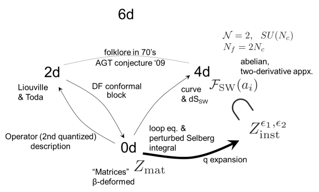
Figure 3: Bird view of the 2d-4d connection through matrices

4.5 more recent developments

The list of papers which discuss subjects closely related to that of this subsection include [352, 353, 354, 355, 356, 357, 358, 359, 360, 361, 362, 262, 363, 301, 364, 365, 366, 367, 368, 369, 370, 371, 372, 373, 374, 375, 376, 377, 378, 379, 380, 381, 382, 383, 384, 385, 386, 387, 388, 389, 390, 391, 392, 393, 394, 395, 396, 397].

We have reviewed the 2d-4d connection from a view point of the matrix model. In this subsection, we comment on some of the more recent developments.

In the last subsection, we have presented the connection between the Virasoro conformal blocks and the four-dimensional $SU(2)$ instanton partition functions via the matrix model and the Selberg integral. This discussion has been generalized in part to that between the $W_{N}$ blocks and the $SU(N)$ partition functions [376].

The both sides also have a natural generalization as a $q$-lift [364]. The Virasoro/$W_{N}$ symmetry in the two-dimensional CFT side is deformed to the $q$-deformed Virasoro/$W_{N}$ symmetry while the four-dimensional $SU(N)$ gauge theory is lifted to the five-dimensional theory. It is interesting to consider the root of unity limit $q\to e^{\frac{2\pi\mathrm{i}}{r}}$ of the $q$-Virasoro/W_N algebras. The appropriate limiting procedure [386, 391] to the root of unity exhibits the connection between the super Virasoro ($r=2$) or the $\textbf{Z}_{r}$-parafermionic CFT and the gauge theory on $\textbf{R}^{4}/\textbf{Z}_{r}$ [368, 370].

There are several pieces of work [363, 301, 379, 384] which prove the 2d-4d connection. The explicit identification can be established in the case of $\beta=1$ [366, 367]. In order to apply to the $\beta\neq 1$ case, the conformal blocks have to be expanded by the generalized Jack polynomial [385] that modifies the standard one. For some lower rank cases, this has been explicitly constructed [388].

References

- [1] K. G. Wilson and J. Kogut, “The renormalization group and the expansion,” Phys. Rep. 12(2), 75–199 (1974).
- [2] M. E. Peskin and D. V. Schroeder, An introduction to quantum field theory, (Westview, 1995).
- [3] N. Seiberg and E. Witten, “Electric - magnetic duality, monopole condensation, and confinement in supersymmetric Yang-Mills theory,” Nucl. Phys. B 426, 19–52, [Erratum-ibid. B 430, 485-486] (1994), arXiv:hep-th/9407087.
- [4] N. Seiberg and E. Witten, “Monopoles, duality and chiral symmetry breaking in supersymmetric QCD,” Nucl. Phys. B 431, 484–550 (1994), arXiv:hep-th/9408099.
- [5] A. Klemm, W. Lerche, S. Yankielowicz, and S. Theisen, “Simple singularities and supersymmetric Yang-Mills theory,” Phys. Lett. B 344, 169–175 (1995), arXiv:hep-th/9411048.
- [6] P. C. Argyres and A. E. Faraggi, “The vacuum structure and spectrum of supersymmetric gauge theory,” Phys. Rev. Lett. 74, 3931–3934 (1995), arXiv:hep-th/9411057.
- [7] A. Hanany and Y. Oz, “On the quantum moduli space of vacua of supersymmetric gauge theories,” Nucl. Phys. B 452, 283–312 (1995), arXiv:hep-th/9505075.
- [8] P. C. Argyres, M. R. Plesser, and A. D. Shapere, “The Coulomb phase of supersymmetric QCD,” Phys. Rev. Lett. 75, 1699–1702 (1995), arXiv:hep-th/9505100.
- [9] P. C. Argyres and A. D. Shapere, “The Vacuum structure of superQCD with classical gauge groups,” Nucl. Phys. B 461, 437–459 (1996), arXiv:hep-th/9509175.
- [10] Y. Tachikawa and S. Terashima, “Seiberg-Witten Geometries Revisited,” JHEP 1109, 010 (2011), arXiv:1108.2315.
- [11] I. M. Krichever, “Methods of algebraic geometry in the theory of non-linear equations,” Russian Math. Surveys 32(6), 185–213 (1977).
- [12] I. M. Krichever, “Integration of nonlinear equations by the methods of algebraic geometry,” Funct. Anal. Appl. 11(1), 12–26 (1977).
- [13] M. A. Olshanetsky and A. M. Perelomov, “Classical integrable finite-dimensional systems related to lie algebras,” Phys. Rep. 71(5), 313–400 (1981).
- [14] A. Gorsky, I. Krichever, A. Marshakov, A. Mironov, and A. Morozov, “Integrability and Seiberg-Witten exact solution,” Phys. Lett. B 355, 466–474 (1995), arXiv:hep-th/9505035.
- [15] E. J. Martinec and N. P. Warner, “Integrable systems and supersymmetric gauge theory,” Nucl. Phys. B 459, 97–112 (1996), arXiv:hep-th/9509161.
- [16] T. Nakatsu and K. Takasaki, “Whitham-Toda hierarchy and supersymmetric Yang-Mills theory,” Mod. Phys. Lett. A 11, 157–168 (1996), arXiv:hep-th/9509162.
- [17] R. Donagi and E. Witten, “Supersymmetric Yang-Mills theory and integrable systems,” Nucl. Phys. B 460, 299–334 (1996), arXiv:hep-th/9510101.
- [18] T. Eguchi and S. K. Yang, “Prepotentials of supersymmetric gauge theories and soliton equations,” Mod. Phys. Lett. A 11, 131–138 (1996), arXiv:hep-th/9510183.
- [19] E. J. Martinec, “Integrable structures in supersymmetric gauge and string theory,” Phys. Lett. B 367, 91–96 (1996), arXiv:hep-th/9510204.
- [20] A. Gorsky and A. Marshakov, “Towards effective topological gauge theories on spectral curves,” Phys. Lett. B 375, 127–134 (1996), arXiv:hep-th/9510224.
- [21] E. J. Martinec and N. P. Warner, “Integrability in gauge theory: A Proof,” (1995), arXiv:hep-th/9511052.
- [22] H. Itoyama and A. Morozov, “Integrability and Seiberg-Witten theory: Curves and periods,” Nucl. Phys. B 477, 855–877 (1996), arXiv:hep-th/9511126.
- [23] C. Gomez, R. Hernandez, and E. Lopez, “S duality and the Calabi-Yau interpretation of the to flow,” Phys. Lett. B 386, 115–122 (1996), arXiv:hep-th/9512017.
- [24] H. Itoyama and A. Morozov, “Prepotential and the Seiberg-Witten theory,” Nucl. Phys. B 491, 529–573 (1997), arXiv:hep-th/9512161.
- [25] H. Itoyama and A. Morozov, “Integrability and Seiberg-Witten theory,”, In Toyonaka 1995, Frontiers in quantum field theory 301-324, Proceedings, International Conference in Honor of Keiji Kikkawa’s 60th Birthday, Toyonaka, Japan, December 14-17, (1995), arXiv:hep-th/9601168.
- [26] A. Levin and M. Olshanetsky, “Double coset construction of moduli space of holomorphic bundles and Hitchin systems,” Commun. Math. Phys. 188, 449–466 (1997), arXiv:alg-geom/9605005.
- [27] E. Witten, “Two-dimensional gravity and intersection theory on moduli space,” Surveys Diff. Geom. 1, 243–310 (1991).
- [28] R. Dijkgraaf, H. L. Verlinde, and E. P. Verlinde, “Topological strings in ,” Nucl. Phys. B 352, 59–86 (1991).
- [29] A. Marshakov, A. Mironov, and A. Morozov, “WDVV - like equations in SUSY Yang-Mills theory,” Phys. Lett. B 389, 43–52 (1996), arXiv:hep-th/9607109.
- [30] H. Itoyama and A. Morozov, “The Dijkgraaf-Vafa prepotential in the context of general Seiberg-Witten theory,” Nucl. Phys. B 657, 53–78 (2003), arXiv:hep-th/0211245.
- [31] A. Marshakov, Seiberg-Witten theory and integrable systems, (World Scientific, 1999).
- [32] M. Matone, “Instantons and recursion relations in SUSY gauge theory,” Phys. Lett. B 357, 342–348 (1995), arXiv:hep-th/9506102.
- [33] C. Ahn and S. Nam, “Integrable structure in supersymmetric gauge theories with massive hypermultiplets,” Phys. Lett. B 387, 304–309 (1996), arXiv:hep-th/9603028.
- [34] A. Gorsky, A. Marshakov, A. Mironov, and A. Morozov, “ supersymmetric QCD and integrable spin chains: Rational case ,” Phys. Lett. B 380, 75–80 (1996), arXiv:hep-th/9603140.
- [35] A. Gorsky, A. Marshakov, A. Mironov, and A. Morozov, “A Note on spectral curve for the periodic homogeneous XYZ spin chain,” (1996), arXiv:hep-th/9604078.
- [36] G. Bonelli and M. Matone, “Nonperturbative relations in SUSY Yang-Mills and WDVV equation,” Phys. Rev. Lett. 77, 4712–4715 (1996), arXiv:hep-th/9605090.
- [37] N. Seiberg and E. Witten, “Gauge dynamics and compactification to three-dimensions,” (1996), arXiv:hep-th/9607163.
- [38] C. Gomez, R. Hernandez, and E. Lopez, “K3 fibrations and softly broken supersymmetric gauge theories,” Nucl. Phys. B 501, 109–133 (1997), arXiv:hep-th/9608104.
- [39] E. D’Hoker, I. M. Krichever, and D. H. Phong, “The Effective prepotential of supersymmetric gauge theories,” Nucl. Phys. B 489, 179–210 (1997), arXiv:hep-th/9609041.
- [40] N. Nekrasov, “Five dimensional gauge theories and relativistic integrable systems,” Nucl. Phys. B 531, 323–344 (1998), arXiv:hep-th/9609219.
- [41] G. Bonelli, M. Matone, and M. Tonin, “Solving SYM by reflection symmetry of quantum vacua,” Phys. Rev. D 55, 6466–6470 (1997), arXiv:hep-th/9610026.
- [42] R. Y. Donagi, “Seiberg-Witten integrable systems,” (1997), arXiv:alg-geom/9705010.
- [43] A. Klemm, “On the geometry behind supersymmetric effective actions in four-dimensions,” (1997), arXiv:hep-th/9705131.
- [44] E. D’Hoker and D. H. Phong, “Calogero-Moser systems in Seiberg-Witten theory,” Nucl. Phys. B 513, 405–444 (1998), arXiv:hep-th/9709053.
- [45] A. Gorsky, S. Gukov, and A. Mironov, “SUSY field theories, integrable systems and their stringy / brane origin. 2.,” Nucl. Phys. B 518, 689–713 (1998), arXiv:hep-th/9710239.
- [46] C. Gomez and R. Hernandez, “Fields, strings and branes,” Lect. Notes Math. 1776, 39–191 (2002), arXiv:hep-th/9711102.
- [47] A. Marshakov and A. Mironov, “5-d and 6-d supersymmetric gauge theories: Prepotentials from integrable systems,” Nucl. Phys. B 518, 59–91 (1998), arXiv:hep-th/9711156.
- [48] H. Kanno and Y. Ohta, “Picard-Fuchs equation and prepotential of five-dimensional SUSY gauge theory compactified on a circle,” Nucl. Phys. B 530, 73–98 (1998), arXiv:hep-th/9801036.
- [49] E. D’Hoker and D. H. Phong, “Spectral curves for superYang-Mills with adjoint hypermultiplet for general Lie algebras,” Nucl. Phys. B 534, 697–719 (1998), arXiv:hep-th/9804126.
- [50] H. W. Braden, A. Marshakov, A. Mironov, and A. Morozov, “Seiberg-Witten theory for a nontrivial compactification from five-dimensions to four-dimensions,” Phys. Lett. B 448, 195–202 (1999), arXiv:hep-th/9812078.
- [51] H. W. Braden, A. Marshakov, A. Mironov, and A. Morozov, “The Ruijsenaars-Schneider model in the context of Seiberg-Witten theory,” Nucl. Phys. B 558, 371–390 (1999), arXiv:hep-th/9902205.
- [52] V. Fock, A. Gorsky, N. Nekrasov, and V. Rubtsov, “Duality in integrable systems and gauge theories,” JHEP 0007, 028 (2000), arXiv:hep-th/9906235.
- [53] H. W. Braden, A. Marshakov, A. Mironov, and A. Morozov, “On double elliptic integrable systems. 1. A Duality argument for the case of ,” Nucl. Phys. B 573, 553–572 (2000), arXiv:hep-th/9906240.
- [54] A. Mironov and A. Morozov, “Commuting Hamiltonians from Seiberg-Witten theta functions,” Phys. Lett. B 475, 71–76 (2000), arXiv:hep-th/9912088.
- [55] J. C. Hurtubise and E. Markman, “Calogero-Moser systems and Hitchen systems,” Commun. Math. Phys. 223, 533–552 (2001), arXiv:math/9912161.
- [56] H. W. Braden and A. Marshakov, “Singular phases of Seiberg-Witten integrable systems: Weak and strong coupling,” Nucl. Phys. B 595, 417–466 (2001), arXiv:hep-th/0009060.
- [57] A. Gorsky and A. Mironov, “Integrable many body systems and gauge theories,” In Aratyn, H. (ed.) et al.: Integrable hierarchies and modern physical theories 33-176 (2000), arXiv:hep-th/0011197.
- [58] I. M. Krichever, “The -function of the universal Whitham hierarchy, matrix models and topological field theories,” Commun. Pure Appl. Math. 47, 437 (1994), arXiv:hep-th/9205110.
- [59] B. A. Dubrovin, “Hamiltonian formalism of Whitham type hierarchies and topological Landau-Ginsburg models,” Commun. Math. Phys. 145, 195–207 (1992).
- [60] S. Aoyama and Y. Kodama, “Topological Landau-Ginzburg theory with a rational potential and the dispersionless KP hierarchy,” Commun. Math. Phys. 182, 185–220 (1996), arXiv:hep-th/9505122.
- [61] A. Cappelli, P. Valtancoli, and L. Vergnano, “Isomonodromic properties of the Seiberg-Witten solution,” Nucl. Phys. B 524, 469–501 (1998), arXiv:hep-th/9710248.
- [62] T. Kubota and N. Yokoi, “Renormalization group flow near the superconformal points in supersymmetric gauge theories,” Prog. Theor. Phys. 100, 423–436 (1998), arXiv:hep-th/9712054.
- [63] R. W. Carroll, “Remarks on Whitham and RG,” (1997), arXiv:hep-th/9712110.
- [64] A. Gorsky, A. Marshakov, A. Mironov, and A. Morozov, “RG equations from Whitham hierarchy,” Nucl. Phys. B 527, 690–716 (1998), arXiv:hep-th/9802007.
- [65] J. D. Edelstein, M. Marino, and J. Mas, “Whitham hierarchies, instanton corrections and soft supersymmetry breaking in superYang-Mills theory,” Nucl. Phys. B 541, 671–697 (1999), arXiv:hep-th/9805172.
- [66] A. Morozov, “Whitham integrability in Seiberg-Witten theory,” (1998), arXiv:hep-th/9903087.
- [67] K. Takasaki, “Whitham deformations and tau functions in supersymmetric gauge theories,” Prog. Theor. Phys. Suppl. 135, 53–74 (1999), arXiv:hep-th/9905224.
- [68] J. D. Edelstein, M. Gomez-Reino, M. Marino, and J. Mas, “ supersymmetric gauge theories with massive hypermultiplets and the Whitham hierarchy,” Nucl. Phys. B 574, 587–619 (2000), arXiv:hep-th/9911115.
- [69] M. Mineev-Weinstein and A. Zabrodin, “Whitham-Toda hierarchy in the Laplacian growth problem,” J.Nonlin.Math.Phys. 8, 212–218 (2001), arXiv:solv-int/9912012.
- [70] I. Antoniadis, H. Partouche, and T. R. Taylor, “Spontaneous breaking of global supersymmetry,” Phys. Lett. B 372, 83–87 (1996), arXiv:hep-th/9512006.
- [71] I. Antoniadis and T. R. Taylor, “Dual SUSY breaking,” Fortsch.Phys. 44, 487–492 (1996), arXiv:hep-th/9604062.
- [72] K. Fujiwara, H. Itoyama, and M. Sakaguchi, “Supersymmetric gauge model and partial breaking of supersymmetry,” Prog. Theor. Phys. 113, 429–455 (2005), arXiv:hep-th/0409060.
- [73] K. Fujiwara, H. Itoyama, and M. Sakaguchi, “ gauge model and partial breaking of supersymmetry,” In Supersymmetry and unification of fundamental interactions. Proceedings, 12th International Conference, SUSY 2004, - (2004), arXiv:hep-th/0410132.
- [74] K. Fujiwara, H. Itoyama, and M. Sakaguchi, “Partial breaking of supersymmetry and of gauge symmetry in the gauge model,” Nucl. Phys. B 723, 33–52 (2005), arXiv:hep-th/0503113.
- [75] H. Itoyama and N. Maru, “D-term Dynamical Supersymmetry Breaking Generating Split Gaugino Masses of Mixed Majorana-Dirac Type,” Int. J. Mod. Phys. A 27, 1250159 (2012), arXiv:1109.2276.
- [76] H. Itoyama and N. Maru, “D-term Triggered Dynamical Supersymmetry Breaking,” Phys. Rev. D 88(2), 025012 (2013), arXiv:1301.7548.
- [77] G. Veneziano and S. Yankielowicz, “An Effective Lagrangian for the Pure Supersymmetric Yang-Mills Theory,” Phys. Lett. B 113, 231 (1982).
- [78] T. R. Taylor, G. Veneziano, and S. Yankielowicz, “Supersymmetric qcd and its massless limit: an effective lagrangian analysis,” Nucl. Phys. B 218(2), 493–513 (1983).
- [79] V. A. Novikov, M. A. Shifman, A. I. Vainshtein, and V. I. Zakharov, “Instanton Effects in Supersymmetric Theories,” Nucl. Phys. B 229, 407 (1983).
- [80] K. Konishi, “Anomalous Supersymmetry Transformation of Some Composite Operators in SQCD,” Phys. Lett. B 135, 439 (1984).
- [81] N. Seiberg, “Supersymmetry and Nonperturbative beta Functions,” Phys. Lett. B 206, 75 (1988).
- [82] V. A. Novikov, M. A. Shifman, A. I. Vainshtein, and V. I. Zakharov, “Nonrenormalization Theorems for Nonperturbative Effects in SUSY Gauge Theories,” Phys. Lett. B 217, 103 (1989).
- [83] K. A. Intriligator, R.G. Leigh, and N. Seiberg, “Exact superpotentials in four-dimensions,” Phys. Rev. D 50, 1092–1104 (1994), arXiv:hep-th/9403198.
- [84] M. R. Douglas and S. H. Shenker, “Dynamics of supersymmetric gauge theory,” Nucl. Phys. B 447, 271–296 (1995), arXiv:hep-th/9503163.
- [85] S. Elitzur, A. Forge, A. Giveon, K. A. Intriligator, and E. Rabinovici, “Massless monopoles via confining phase superpotentials,” Phys. Lett. B 379, 121–125 (1996), arXiv:hep-th/9603051.
- [86] S. Terashima and S.-K. Yang, “ADE confining phase superpotentials,” Nucl. Phys. B 519, 453–469 (1998), arXiv:hep-th/9706076.
- [87] S. Gukov, C. Vafa, and E. Witten, “CFT’s from Calabi-Yau four folds,” Nucl. Phys. B 584, 69–108 (2000), arXiv:hep-th/9906070.
- [88] F. Cachazo, K. A. Intriligator, and C. Vafa, “A Large N duality via a geometric transition,” Nucl. Phys. B 603, 3–41 (2001), arXiv:hep-th/0103067.
- [89] F. Cachazo and C. Vafa, “ and geometry from fluxes,” (2002), arXiv:hep-th/0206017.
- [90] R. Dijkgraaf and C. Vafa, “Matrix models, topological strings, and supersymmetric gauge theories,” Nucl. Phys. B 644, 3–20 (2002), arXiv:hep-th/0206255.
- [91] R. Dijkgraaf and C. Vafa, “On geometry and matrix models,” Nucl. Phys. B 644, 21–39 (2002), arXiv:hep-th/0207106.
- [92] R. Dijkgraaf and C. Vafa, “A Perturbative window into nonperturbative physics,” (2002), arXiv:hep-th/0208048.
- [93] L. Chekhov and A. Mironov, “Matrix models versus Seiberg-Witten / Whitham theories,” Phys. Lett. B 552, 293–302 (2003), arXiv:hep-th/0209085.
- [94] F. Ferrari, “On exact superpotentials in confining vacua,” Nucl. Phys. B 648, 161–173 (2003), arXiv:hep-th/0210135.
- [95] F. Ferrari, “Quantum parameter space and double scaling limits in superYang-Mills theory,” Phys. Rev. D 67, 085013 (2003), arXiv:hep-th/0211069.
- [96] H. Itoyama and A. Morozov, “Experiments with the WDVV equations for the gluino condensate prepotential: The Cubic (two cut) case,” Phys. Lett. B 555, 287–295 (2003), arXiv:hep-th/0211259.
- [97] H. Itoyama and A. Morozov, “Calculating gluino condensate prepotential,” Prog. Theor. Phys. 109, 433–463 (2003), arXiv:hep-th/0212032.
- [98] M. Matone, “Seiberg-Witten duality in Dijkgraaf-Vafa theory,” Nucl. Phys. B 656, 78–92 (2003), arXiv:hep-th/0212253.
- [99] L. Chekhov, A. Marshakov, A. Mironov, and D. Vasiliev, “DV and WDVV,” Phys. Lett. B 562, 323–338 (2003), arXiv:hep-th/0301071.
- [100] H. Itoyama and A. Morozov, “Gluino condensate (CIV-DV) prepotential from its Whitham time derivatives,” Int. J. Mod. Phys. A 18, 5889–5906 (2003), arXiv:hep-th/0301136.
- [101] R. Boels, J. de Boer, R. Duivenvoorden, and J. Wijnhout, “Nonperturbative superpotentials and compactification to three-dimensions,” JHEP 0403, 009 (2004), arXiv:hep-th/0304061.
- [102] T. J. Hollowood, “Critical points of glueball superpotentials and equilibria of integrable systems,” JHEP 0310, 051 (2003), arXiv:hep-th/0305023.
- [103] R. Boels, J. de Boer, R. Duivenvoorden, and J. Wijnhout, “Factorization of Seiberg-Witten curves and compactification to three-dimensions,” JHEP 0403, 010 (2004), arXiv:hep-th/0305189.
- [104] A.S. Alexandrov, A. Mironov, and A. Morozov, “Partition functions of matrix models as the first special functions of string theory. 1. Finite size Hermitean one matrix model,” Int. J. Mod. Phys. A 19, 4127–4165 (2004), arXiv:hep-th/0310113.
- [105] H. Itoyama and H. Kanno, “Whitham prepotential and superpotential,” Nucl. Phys. B 686, 155–164 (2004), arXiv:hep-th/0312306.
- [106] L. Girardello, A. Mariotti, and G. Tartaglino-Mazzucchelli, “On supersymmetry breaking and the Dijkgraaf-Vafa conjecture,” JHEP 0603, 104 (2006), arXiv:hep-th/0601078.
- [107] N. Dorey, T. J. Hollowood, S. P. Kumar, and A. Sinkovics, “Exact superpotentials from matrix models,” JHEP 0211, 039 (2002), arXiv:hep-th/0209089.
- [108] N. Dorey, T. J. Hollowood, S. P. Kumar, and A. Sinkovics, “Massive vacua of theory and duality from matrix models,” JHEP 0211, 040 (2002), arXiv:hep-th/0209099.
- [109] H. Fuji and Y. Ookouchi, “Comments on effective superpotentials via matrix models,” JHEP 0212, 067 (2002), arXiv:hep-th/0210148.
- [110] D. Berenstein, “Quantum moduli spaces from matrix models,” Phys. Lett. B 552, 255–264 (2003), arXiv:hep-th/0210183.
- [111] N. Dorey, T. J. Hollowood, and S. P. Kumar, “S duality of the Leigh-Strassler deformation via matrix models,” JHEP 0212, 003 (2002), arXiv:hep-th/0210239.
- [112] A. Gorsky, “Konishi anomaly and effective superpotentials from matrix models,” Phys. Lett. B 554, 185–189 (2003), arXiv:hep-th/0210281.
- [113] R. Argurio, V. L. Campos, G. Ferretti, and R. Heise, “Exact superpotentials for theories with flavors via a matrix integral,” Phys. Rev. D 67, 065005 (2003), arXiv:hep-th/0210291.
- [114] J. McGreevy, “Adding flavor to Dijkgraaf-Vafa,” JHEP 0301, 047 (2003), arXiv:hep-th/0211009.
- [115] I. Bena and R. Roiban, “Exact superpotentials in N = 1 theories with flavor and their matrix model formulation,” Phys. Lett. B 555, 117–125 (2003), arXiv:hep-th/0211075.
- [116] M. Aganagic, A. Klemm, M. Marino, and C. Vafa, “Matrix model as a mirror of Chern-Simons theory,” JHEP 0402, 010 (2004), arXiv:hep-th/0211098.
- [117] R. Gopakumar, “ theories and a geometric master field,” JHEP 0305, 033 (2003), arXiv:hep-th/0211100.
- [118] B. Feng, “Seiberg Duality in Matrix Model,” (2002), arXiv:hep-th/0211202.
- [119] A. Klemm, M. Marino, and S. Theisen, “Gravitational corrections in supersymmetric gauge theory and matrix models,” JHEP 0303, 051 (2003), arXiv:hep-th/0211216.
- [120] V. A. Kazakov and A. Marshakov, “Complex curve of the two matrix model and its tau function,” J. Phys. A 36, 3107–3136 (2003), arXiv:hep-th/0211236.
- [121] S. G. Naculich, H. J. Schnitzer, and N. Wyllard, “Matrix model approach to the gauge theory with matter in the fundamental representation,” JHEP 0301, 015 (2003), arXiv:hep-th/0211254.
- [122] S. Aoyama and T. Masuda, “The Whitham deformation of the Dijkgraaf-Vafa theory,” JHEP 0403, 072 (2004), arXiv:hep-th/0309232.
- [123] R. Argurio, G. Ferretti, and R. Heise, “An Introduction to supersymmetric gauge theories and matrix models,” Int. J. Mod. Phys. A 19, 2015–2078 (2004), arXiv:hep-th/0311066.
- [124] R. Dijkgraaf, S. Gukov, V. A. Kazakov, and C. Vafa, “Perturbative analysis of gauged matrix models,” Phys. Rev. D 68, 045007 (2003), arXiv:hep-th/0210238.
- [125] R. Dijkgraaf, M. T. Grisaru, C. S. Lam, C. Vafa, and D. Zanon, “Perturbative computation of glueball superpotentials,” Phys. Lett. B 573, 138–146 (2003), arXiv:hep-th/0211017.
- [126] H. Suzuki, “Perturbative derivation of exact superpotential for meson fields from matrix theories with one flavor,” JHEP 0303, 005 (2003), arXiv:hep-th/0211052.
- [127] Y. Demasure and R. A. Janik, “Effective matter superpotentials from Wishart random matrices,” Phys. Lett. B 553, 105–108 (2003), arXiv:hep-th/0211082.
- [128] S. G. Naculich, H. J. Schnitzer, and N. Wyllard, “The gauge theory prepotential and periods from a perturbative matrix model calculation,” Nucl. Phys. B 651, 106–124 (2003), arXiv:hep-th/0211123.
- [129] A. Dymarsky and V. Pestun, “On the property of Cachazo-Intriligator-Vafa prepotential at the extremum of the superpotential,” Phys. Rev. D 67, 125001 (2003), arXiv:hep-th/0301135.
- [130] H. Kawai, T. Kuroki, and T. Morita, “Dijkgraaf-Vafa theory as large reduction,” Nucl. Phys. B 664, 185–212 (2003), arXiv:hep-th/0303210.
- [131] M. Gomez-Reino, “Exact superpotentials, theories with flavor and confining vacua,” JHEP 0406, 051 (2004), arXiv:hep-th/0405242.
- [132] S. Aoyama, “The Disc amplitude of the Dijkgraaf-Vafa theory: expansion vs complex curve analysis,” JHEP 0510, 032 (2005), arXiv:hep-th/0504162.
- [133] L. Hollands, J. Marsano, K. Papadodimas, and M. Shigemori, “Nonsupersymmetric Flux Vacua and Perturbed Systems,” JHEP 0810, 102 (2008), arXiv:0804.4006.
- [134] S. Cecotti, L. Girardello, and M. Porrati, “CONSTRAINTS ON PARTIAL SUPERHIGGS,” Nucl. Phys. B 268, 295–316 (1986).
- [135] S. Cecotti, L. Girardello, and M. Porrati, “An Exceptional Supergravity With Flat Potential and Partial Superhiggs,” Phys. Lett. B 168, 83 (1986).
- [136] J. Hughes and J. Polchinski, “Partially Broken Global Supersymmetry and the Superstring,” Nucl. Phys. B 278, 147 (1986).
- [137] J. Hughes, J. Liu, and J. Polchinski, “Supermembranes,” Phys. Lett. B 180, 370 (1986).
- [138] S. Ferrara, L. Girardello, and M. Porrati, “Minimal Higgs branch for the breaking of half of the supersymmetries in supergravity,” Phys. Lett. B 366, 155–159 (1996), arXiv:hep-th/9510074.
- [139] S. Ferrara, L. Girardello, and M. Porrati, “Spontaneous breaking of to in rigid and local supersymmetric theories,” Phys. Lett. B 376, 275–281 (1996), arXiv:hep-th/9512180.
- [140] L. Álvarez-Gaumé, J. Distler, C. Kounnas, and M. Mariño, “Softly broken QCD,” Int. J. Mod. Phys. A 11, 4745–4777 (1996), arXiv:hep-th/9604004.
- [141] M. Porrati, “Spontaneous breaking of extended supersymmetry in global and local theories,” Nucl. Phys. Proc. Suppl. 55B, 240–244 (1997), arXiv:hep-th/9609073.
- [142] H. Partouche and B. Pioline, “Partial spontaneous breaking of global supersymmetry,” Nucl. Phys. Proc. Suppl. 56B, 322–327 (1997), arXiv:hep-th/9702115.
- [143] E. A. Ivanov and B. M. Zupnik, “Modified supersymmetry and Fayet-Iliopoulos terms,” Phys. Atom. Nucl. 62, 1043–1055 (1999), arXiv:hep-th/9710236.
- [144] T. R. Taylor and C. Vafa, “RR flux on Calabi-Yau and partial supersymmetry breaking,” Phys. Lett. B 474, 130–137 (2000), arXiv:hep-th/9912152.
- [145] F. Cachazo, M. R. Douglas, N. Seiberg, and E. Witten, “Chiral rings and anomalies in supersymmetric gauge theory,” JHEP 0212, 071 (2002), arXiv:hep-th/0211170.
- [146] Y. Tachikawa, “Derivation of the Konishi anomaly relation from Dijkgraaf-Vafa with (Bi)fundamental matters,” Phys. Lett. B 573, 235–238 (2003), arXiv:hep-th/0211189.
- [147] F. Cachazo, N. Seiberg, and E. Witten, “Phases of supersymmetric gauge theories and matrices,” JHEP 0302, 042 (2003), arXiv:hep-th/0301006.
- [148] H. Itoyama and H. Kanno, “Supereigenvalue model and Dijkgraaf-Vafa proposal,” Phys. Lett. B 573, 227–234 (2003), arXiv:hep-th/0304184.
- [149] J. R. David, E. Gava, and K. S. Narain, “Konishi anomaly approach to gravitational terms,” JHEP 0309, 043 (2003), arXiv:hep-th/0304227.
- [150] L. F. Alday, M. Cirafici, J. R. David, E. Gava, and K. S. Narain, “Gravitational terms through anomaly equations and deformed chiral rings,” JHEP 0401, 001 (2004), arXiv:hep-th/0305217.
- [151] P. Kaste and H. Partouche, “On the equivalence of brane worlds and geometric singularities with flux,” JHEP 0411, 033 (2004), arXiv:hep-th/0409303.
- [152] K. Fujiwara, H. Itoyama, and M. Sakaguchi, “Partial supersymmetry breaking and gauge model with hypermultiplets in harmonic superspace,” Nucl. Phys. B 740, 58–78 (2006), arXiv:hep-th/0510255.
- [153] P. Merlatti, “Fractional branes and the gravity dual of partial supersymmetry breaking,” Nucl. Phys. B 744, 207–220 (2006), arXiv:hep-th/0511280.
- [154] F. Ferrari, “The Proof of the Dijkgraaf-Vafa conjecture and application to the mass gap and confinement problems,” JHEP 0606, 039 (2006), arXiv:hep-th/0602249.
- [155] K. Fujiwara, H. Itoyama, and M. Sakaguchi, “Supersymmetric gauge model and partial breaking of supersymmetry,” Prog. Theor. Phys. Suppl. 164, 125–137 (2007), arXiv:hep-th/0602267.
- [156] H. Itoyama and K. Maruyoshi, “ gauged supergravity and partial breaking of local supersymmetry,” Int. J. Mod. Phys. A 21, 6191–6210 (2006), arXiv:hep-th/0603180.
- [157] K. Fujiwara, “Partial Breaking of Supersymmetry and Decoupling Limit of Nambu-Goldstone Fermion in Gauge Model,” Nucl. Phys. B 770, 145–153 (2007), arXiv:hep-th/0609039.
- [158] K. Fujiwara, H. Itoyama, and M. Sakaguchi, “Spontaneous partial breaking of supersymmetry and the gauge model,” AIP Conf. Proc. 903, 521–524 (2007), arXiv:hep-th/0611284.
- [159] A. Marshakov and N. Nekrasov, “Extended Seiberg-Witten Theory and Integrable Hierarchy,” JHEP 0701, 104 (2007), arXiv:hep-th/0612019.
- [160] F. Ferrari, “The Chiral ring and the periods of the resolvent,” Nucl. Phys. B 770, 371–383 (2007), arXiv:hep-th/0701220.
- [161] H. Itoyama and K. Maruyoshi, “Deformation of Dijkgraaf-Vafa Relation via Spontaneously Broken Supersymmetry,” Phys. Lett. B 650, 298–303 (2007), arXiv:0704.1060.
- [162] F. Ferrari, “Extended super Yang-Mills theory,” JHEP 0711, 001 (2007), arXiv:0709.0472.
- [163] H. Itoyama, K. Maruyoshi, and M. Sakaguchi, “ quiver gauge model and partial supersymmetry breaking,” Nucl. Phys. B 794, 216–230 (2008), arXiv:0709.3166.
- [164] K. Maruyoshi, “Effective superpotential and partial breaking of supersymmetry,” (2007), arXiv:0710.2154.
- [165] F. Ferrari and V. Wens, “Consistency conditions in the chiral ring of super Yang-Mills theories,” Nucl. Phys. B 798, 470–490 (2008), arXiv:0710.2978.
- [166] H. Itoyama and K. Maruyoshi, “Deformation of Dijkgraaf-Vafa Relation via Spontaneously Broken Supersymmetry II,” Nucl. Phys. B 796, 246–261 (2008), arXiv:0710.4377.
- [167] O. Saito, “The Glueball superpotential for ,” (2007), arXiv:0711.1456.
- [168] F. Ferrari, “The Microscopic Approach to Super Yang-Mills Theories,” Int. J. Mod. Phys. A 23, 2307–2323 (2008), arXiv:0804.0244.
- [169] M. Aganagic, C. Beem, J. Seo, and C. Vafa, “Extended Supersymmetric Moduli Space and a SUSY/Non-SUSY Duality,” Nucl. Phys. B 822, 135–171 (2009), arXiv:0804.2489.
- [170] K. Ohta and T.-S. Tai, “Extended MQCD and SUSY/non-SUSY duality,” JHEP 0809, 033 (2008), arXiv:0806.2705.
- [171] T. Nakatsu, Y. Noma, and K. Takasaki, “Integrable Structure of 5d Supersymmetric Yang-Mills and Melting Crystal,” Int. J. Mod. Phys. A 23, 2332–2342 (2008), arXiv:0806.3675.
- [172] K. Maruyoshi, “Quiver Gauge Theory and Extended Electric-magnetic Duality,” JHEP 0909, 061 (2009), arXiv:0904.2431.
- [173] H. Itoyama, K. Maruyoshi, and S. Minato, “Low Energy Processes Associated with Spontaneously Broken Supersymmetry,” Nucl. Phys. B 830, 1–16 (2010), arXiv:0909.5486.
- [174] K. Fujiwara and H. Itoyama, “Spontaneous Partial Breaking of Supersymmetry,” Adv.Stud.Pure Math. 55, 223–233 (2009).
- [175] K. Fujikawa, “Path-integral measure for gauge-invariant fermion theories,” Phys. Rev. Lett. 42(18), 1195 (1979).
- [176] K. Fujikawa, “Path integral for gauge theories with fermions,” Phys. Rev. D 21(10), 2848 (1980).
- [177] L. F. Alday, D. Gaiotto, and Y. Tachikawa, “Liouville Correlation Functions from Four-dimensional Gauge Theories,” Lett. Math. Phys. 91, 167–197 (2010), arXiv:0906.3219.
- [178] A. Losev, G. W. Moore, N. Nekrasov, and S. Shatashvili, “Four-dimensional avatars of two-dimensional RCFT,” Nucl. Phys. Proc. Suppl. 46, 130–145 (1996), arXiv:hep-th/9509151.
- [179] A. Losev, N. Nekrasov, and S. L. Shatashvili, “Issues in topological gauge theory,” Nucl. Phys. B 534, 549–611 (1998), arXiv:hep-th/9711108.
- [180] H. Nakajima, Lectures on Hilbert schemes of points on surfaces, volume 18, (American Mathematical Society Providence, 1999).
- [181] N. A. Nekrasov, “Seiberg-Witten prepotential from instanton counting,” Adv. Theor. Math. Phys. 7, 831–864 (2004), arXiv:hep-th/0206161.
- [182] R. Flume and R. Poghossian, “An Algorithm for the microscopic evaluation of the coefficients of the Seiberg-Witten prepotential,” Int. J. Mod. Phys. A 18, 2541 (2003), arXiv:hep-th/0208176.
- [183] H. Nakajima and K. Yoshioka, “Instanton counting on blowup. 1.,” Invent. Math. 162, 313–355 (2005), arXiv:math/0306198.
- [184] N. Nekrasov and A. Okounkov, “Seiberg-Witten theory and random partitions,”, Prog. Math. 244, 525-596, ed. by P. Etingof, V. Retakh and I.M. Singer, Birkh (2003), arXiv:hep-th/0306238.
- [185] H. Nakajima and K. Yoshioka, “Lectures on instanton counting,” Algebraic structures and moduli spaces 38, 31–101 (2004).
- [186] H. Nakajima and K. Yoshioka, “Instanton counting on blowup. II. K-theoretic partition function,” (2005), arXiv:math/0505553.
- [187] E. Brezin, C. Itzykson, G. Parisi, and J. B. Zuber, “Planar Diagrams,” Commun. Math. Phys. 59, 35 (1978).
- [188] E. Brezin and V. A. Kazakov, “Exactly Solvable Field Theories of Closed Strings,” Phys. Lett. B 236, 144–150 (1990).
- [189] M. R. Douglas and S. H. Shenker, “Strings in Less Than One-Dimension,” Nucl. Phys. B 335, 635 (1990).
- [190] D. J. Gross and A. A. Migdal, “Nonperturbative Two-Dimensional Quantum Gravity,” Phys. Rev. Lett. 64, 127 (1990).
- [191] D. J. Gross and A. A. Migdal, “A Nonperturbative Treatment of Two-dimensional Quantum Gravity,” Nucl. Phys. B 340, 333–365 (1990).
- [192] A. Mironov and A. Morozov, “On the origin of Virasoro constraints in matrix models: Lagrangian approach,” Phys. Lett. B 252, 47–52 (1990).
- [193] J. Ambjorn, J. Jurkiewicz, and Yu. M. Makeenko, “Multiloop correlators for two-dimensional quantum gravity,” Phys. Lett. B 251, 517–524 (1990).
- [194] F. David, “Loop Equations and Nonperturbative Effects in Two-dimensional Quantum Gravity,” Mod. Phys. Lett. A 5, 1019–1030 (1990).
- [195] G. R. Harris, “Loops and unoriented strings,” Nucl. Phys. B 356, 685–702 (1991).
- [196] J. de Boer, “Multimatrix models and the KP hierarchy,” Nucl. Phys. B 366, 602–628 (1991).
- [197] H. Itoyama and Y. Matsuo, “Noncritical Virasoro algebra of matrix model and quantized string field,” Phys. Lett. B 255, 202–208 (1991).
- [198] H. Itoyama and Y. Matsuo, “ type constraints in matrix models at finite ,” Phys. Lett. B 262, 233–239 (1991).
- [199] A Marshakov, A Mironov, and A Morozov, “Generalized matrix models as conformal field theories discrete case,” Phys. Lett. B 265(1), 99–107 (1991).
- [200] H. Itoyama, “Matrix models at finite ,” (1991), arXiv:hep-th/9111039.
- [201] L. Alvarez-Gaume, H. Itoyama, J. L. Manes, and A. Zadra, “Superloop equations and two-dimensional supergravity,” Int. J. Mod. Phys. A 7, 5337–5368 (1992), arXiv:hep-th/9112018.
- [202] C.-r. Ahn and K. Shigemoto, “One point functions of loops and constraints equations of the multimatrix models at finite N,” Phys. Lett. B 285, 42–48 (1992), arXiv:hep-th/9112057.
- [203] S. Kharchev, A. Marshakov, A. Mironov, A. Morozov, and S. Pakuliak, “Conformal matrix models as an alternative to conventional multimatrix models,” Nucl. Phys. B 404, 717–750 (1993), arXiv:hep-th/9208044.
- [204] I. K. Kostov, “Gauge invariant matrix model for the A-D-E closed strings,” Phys. Lett. B 297, 74–81 (1992), arXiv:hep-th/9208053.
- [205] A. Morozov, “Pair correlator in the Itzykson-Zuber integral,” Mod. Phys. Lett. A 7, 3503–3508 (1992), arXiv:hep-th/9209074.
- [206] A. Morozov Phys. Usp. 35, 671 (1992).
- [207] S. L. Shatashvili, “Correlation functions in the Itzykson-Zuber model,” Commun. Math. Phys. 154, 421–432 (1993), arXiv:hep-th/9209083.
- [208] L. Bonora and C. S. Xiong, “Multimatrix models without continuum limit,” Nucl. Phys. B 405, 191–227 (1993), arXiv:hep-th/9212070.
- [209] J. Ambjorn, L. Chekhov, C. F. Kristjansen, and Yu. Makeenko, “Matrix model calculations beyond the spherical limit,” Nucl. Phys. B 404, 127–172 (1993), arXiv:hep-th/9302014.
- [210] A. Morozov, “Integrability and matrix models,” Phys. Usp. 37, 1–55 (1994), arXiv:hep-th/9303139.
- [211] A. Mironov, “2-d gravity and matrix models. 1. 2-d gravity,” Int. J. Mod. Phys. A 9, 4355–4406 (1994), arXiv:hep-th/9312212.
- [212] H Itoyama, “Loop equation, matrix model and supersymmetry,” Soryushiron Kenkyu 86(4), D8–D23 (1993).
- [213] A. Mironov, A. Morozov, and G.W. Semenoff, “Unitary matrix integrals in the framework of generalized Kontsevich model. 1. Brezin-Gross-Witten model,” Int. J. Mod. Phys. A 11, 5031–5080 (1996), arXiv:hep-th/9404005.
- [214] A. Morozov, “Matrix models as integrable systems,” (1995), arXiv:hep-th/9502091.
- [215] H. Awata, Y. Matsuo, S. Odake, and J. Shiraishi, “A Note on Calogero-Sutherland model, W(n) singular vectors and generalized matrix models,” Soryushiron Kenkyu 91, A69–A75 (1995), arXiv:hep-th/9503028.
- [216] I. K. Kostov, “Solvable statistical models on a random lattice,” Nucl. Phys. Proc. Suppl. 45A, 13–28 (1996), arXiv:hep-th/9509124.
- [217] J. C. Plefka, “Supersymmetric generalizations of matrix models,” (1996), arXiv:hep-th/9601041.
- [218] G. Akemann, “Higher genus correlators for the Hermitian matrix model with multiple cuts,” Nucl. Phys. B 482, 403–430 (1996), arXiv:hep-th/9606004.
- [219] G. Bonnet, F. David, and B. Eynard, “Breakdown of universality in multicut matrix models,” J. Phys. A 33, 6739–6768 (2000), arXiv:cond-mat/0003324.
- [220] S. Seki, “Comments on quiver gauge theories and matrix models,” Nucl. Phys. B 661, 257–272 (2003), arXiv:hep-th/0212079.
- [221] C. Hofman, “SuperYang-Mills with flavors from large matrix models,” JHEP 0310, 022 (2003), arXiv:hep-th/0212095.
- [222] C. I. Lazaroiu, “Holomorphic matrix models,” JHEP 0305, 044 (2003), arXiv:hep-th/0303008.
- [223] A. Klemm, K. Landsteiner, C. I. Lazaroiu, and I. Runkel, “Constructing gauge theory geometries from matrix models,” JHEP 0305, 066 (2003), arXiv:hep-th/0303032.
- [224] R. Casero and E. Trincherini, “Quivers via anomaly chains,” JHEP 0309, 041 (2003), arXiv:hep-th/0304123.
- [225] R. Casero and E. Trincherini, “Phases and geometry of the quiver gauge theory and matrix models,” JHEP 0309, 063 (2003), arXiv:hep-th/0307054.
- [226] S. Chiantese, A. Klemm, and I. Runkel, “Higher order loop equations for and quiver matrix models,” JHEP 0403, 033 (2004), arXiv:hep-th/0311258.
- [227] M. L. Mehta, Random matrices, volume 142, (Academic press, 2004).
- [228] P. Desrosiers, “Duality in random matrix ensembles for all ,” Nucl. Phys. B 817, 224–251 (2009), arXiv:0801.3438.
- [229] B. Eynard and O. Marchal, “Topological expansion of the Bethe ansatz, and non-commutative algebraic geometry,” JHEP 0903, 094 (2009), arXiv:0809.3367.
- [230] R. Dijkgraaf, L. Hollands, and P. Sułkowski, “Quantum Curves and D-Modules,” JHEP 0911, 047 (2009), arXiv:0810.4157.
- [231] A Zabrodin, “Random matrices and laplacian growth,” arXiv:0907.4929[math-ph] (2009).
- [232] N. A. Nekrasov and S. L. Shatashvili, “Quantization of Integrable Systems and Four Dimensional Gauge Theories,” (2009), arXiv:0908.4052.
- [233] H. Itoyama, K. Maruyoshi, and T. Oota, “The Quiver Matrix Model and 2d-4d Conformal Connection,” Prog. Theor. Phys. 123, 957–987 (2010), arXiv:0911.4244.
- [234] R. C. Penner, “The decorated teichmüller space of punctured surfaces,” Commun. Math. Phys. 113(2), 299–339 (1987).
- [235] R. C. Penner, “Perturbative series and the moduli space of Riemann surfaces,” J. Diff. Geom. 27(1), 35–53 (1988).
- [236] E. Witten, “Solutions of four-dimensional field theories via M theory,” Nucl. Phys. B 500, 3–42 (1997), arXiv:hep-th/9703166.
- [237] A. Marshakov, M. Martellini, and A. Morozov, “Insights and puzzles from branes: 4-D SUSY Yang-Mills from 6-D models,” Phys. Lett. B 418, 294–302 (1998), arXiv:hep-th/9706050.
- [238] D. Gaiotto, “ dualities,” JHEP 1208, 034 (2012), arXiv:0904.2715.
- [239] D. Gaiotto and J. Maldacena, “The Gravity duals of superconformal field theories,” JHEP 1210, 189 (2012), arXiv:0904.4466.
- [240] Y. Tachikawa, “Six-dimensional theory and four-dimensional SO-USp quivers,” JHEP 0907, 067 (2009), arXiv:0905.4074.
- [241] F. Benini, S. Benvenuti, and Y. Tachikawa, “Webs of five-branes and superconformal field theories,” JHEP 0909, 052 (2009), arXiv:0906.0359.
- [242] D. Nanopoulos and D. Xie, “ SU Quiver with USP Ends or SU Ends with Antisymmetric Matter,” JHEP 0908, 108 (2009), arXiv:0907.1651.
- [243] N. Wyllard, “ conformal Toda field theory correlation functions from conformal quiver gauge theories,” JHEP 0911, 002 (2009), arXiv:0907.2189.
- [244] N. Drukker, D. R. Morrison, and T. Okuda, “Loop operators and S-duality from curves on Riemann surfaces,” JHEP 0909, 031 (2009), arXiv:0907.2593.
- [245] K. Maruyoshi, M. Taki, S. Terashima, and F. Yagi, “New Seiberg Dualities from Dualities,” JHEP 0909, 086 (2009), arXiv:0907.2625.
- [246] A. Marshakov, A. Mironov, and A. Morozov, “Combinatorial Expansions of Conformal Blocks,” Theor. Math. Phys. 164, 831–852 (2010), arXiv:0907.3946.
- [247] D. Gaiotto, G. W. Moore, and A. Neitzke, “Wall-crossing, Hitchin Systems, and the WKB Approximation,” (2009), arXiv:0907.3987.
- [248] D. Gaiotto, “Asymptotically free theories and irregular conformal blocks,” J. Phys. Conf. Ser. 462(1), 012014 (2013), arXiv:0908.0307.
- [249] A. Mironov, S. Mironov, A. Morozov, and And. Morozov, “CFT exercises for the needs of AGT,” (2009), arXiv:0908.2064.
- [250] A. Mironov and A. Morozov, “The Power of Nekrasov Functions,” Phys. Lett. B 680, 188–194 (2009), arXiv:0908.2190.
- [251] A. Mironov and A. Morozov, “On AGT relation in the case of ,” Nucl. Phys. B 825, 1–37 (2010), arXiv:0908.2569.
- [252] D. V. Nanopoulos and D. Xie, “On Crossing Symmmetry and Modular Invariance in Conformal Field Theory and S Duality in Gauge Theory,” Phys. Rev. D 80, 105015 (2009), arXiv:0908.4409.
- [253] L. F. Alday, D. Gaiotto, S. Gukov, Y. Tachikawa, and H. Verlinde, “Loop and surface operators in gauge theory and Liouville modular geometry,” JHEP 1001, 113 (2010), arXiv:0909.0945.
- [254] N. Drukker, J. Gomis, T. Okuda, and J. Teschner, “Gauge Theory Loop Operators and Liouville Theory,” JHEP 1002, 057 (2010), arXiv:0909.1105.
- [255] F. Benini, Y. Tachikawa, and B. Wecht, “Sicilian gauge theories and dualities,” JHEP 1001, 088 (2010), arXiv:0909.1327.
- [256] A. Marshakov, A. Mironov, and A. Morozov, “On non-conformal limit of the AGT relations,” Phys. Lett. B 682, 125–129 (2009), arXiv:0909.2052.
- [257] R. Dijkgraaf and C. Vafa, “Toda Theories, Matrix Models, Topological Strings, and Gauge Systems,” (2009), arXiv:0909.2453.
- [258] A. Marshakov, A. Mironov, and A. Morozov, “Zamolodchikov asymptotic formula and instanton expansion in SUSY QCD,” JHEP 0911, 048 (2009), arXiv:0909.3338.
- [259] R. Poghossian, “Recursion relations in CFT and SYM theory,” JHEP 0912, 038 (2009), arXiv:0909.3412.
- [260] A. Mironov and A. Morozov, “Proving AGT relations in the large-c limit,” Phys. Lett. B 682, 118–124 (2009), arXiv:0909.3531.
- [261] G. Bonelli and A. Tanzini, “Hitchin systems, gauge theories and W-gravity,” Phys. Lett. B 691, 111–115 (2010), arXiv:0909.4031.
- [262] H. Awata and Y. Yamada, “Five-dimensional AGT Conjecture and the Deformed Virasoro Algebra,” JHEP 1001, 125 (2010), arXiv:0910.4431.
- [263] K. Papadodimas, “Topological Anti-Topological Fusion in Four-Dimensional Superconformal Field Theories,” JHEP 1008, 118 (2010), arXiv:0910.4963.
- [264] A. Mironov and A. Morozov, “Nekrasov Functions and Exact Bohr-Zommerfeld Integrals,” JHEP 1004, 040 (2010), arXiv:0910.5670.
- [265] V. Alba and And. Morozov, “Non-conformal limit of AGT relation from the 1-point torus conformal block,” JETP Lett. 90, 708–712 (2009), arXiv:0911.0363.
- [266] D. Gaiotto, “Surface Operators in N = 2 4d Gauge Theories,” JHEP 1211, 090 (2012), arXiv:0911.1316.
- [267] D. Nanopoulos and D. Xie, “Hitchin Equation, Singularity, and Superconformal Field Theories,” JHEP 1003, 043 (2010), arXiv:0911.1990.
- [268] A. Mironov and A. Morozov, “Nekrasov Functions from Exact BS Periods: The Case of ,” J. Phys. A 43, 195401 (2010), arXiv:0911.2396.
- [269] G. Aminov, H. W. Braden, A. Mironov, A. Morozov, and A. Zotov, “Seiberg-Witten curves and double-elliptic integrable systems,” JHEP 1501, 033 (2015), arXiv:1410.0698.
- [270] D. Galakhov, A. Mironov, and A. Morozov, “Wall Crossing Invariants: from quantum mechanics to knots,” J.Exp.Theor.Phys. 120(3), 549–577 (2015), arXiv:1410.8482.
- [271] A. Selberg, “Remarks on a multiple integral,” Norsk Mat. Tidsskr. 26, 71–78 (1944).
- [272] B. Sutherland, “Exact results for a quantum many body problem in one-dimension,” Phys. Rev. A 4, 2019–2021 (1971).
- [273] B. Sutherland, “Exact results for a quantum many body problem in one-dimension. 2.,” Phys. Rev. A 5, 1372–1376 (1972).
- [274] V. S. Dotsenko and V. A. Fateev, “Conformal algebra and multipoint correlation functions in 2d statistical models,” Nucl. Phys. B 240(3), 312–348 (1984).
- [275] A. A. Belavin, A. M. Polyakov, and A. B. Zamolodchikov, “Infinite Conformal Symmetry in Two-Dimensional Quantum Field Theory,” Nucl. Phys. B 241, 333–380 (1984).
- [276] I. G. Macdonald, “Commuting differential operators and zonal spherical functions,”, In Algebraic groups Utrecht 1986. Springer (1987), Proceedings of a Symposium in Honour of T. A. Springer, Lecture Notes in Math. 1271, 189-200, ed. by A. M. Cohen, W. H. Hesselink, W. L. J. van der Kallen and J. R. Strooker.
- [277] R. P Stanley, “Some combinatorial properties of jack symmetric functions,” Adv. Math. 77(1), 76–115 (1989).
- [278] J. Kaneko, “Selberg integrals and hypergeometric functions associated with jack polynomials,” SIAM J. Math. Anal. 24(4), 1086–1110 (1993).
- [279] H. Awata, Y. Matsuo, S. Odake, and J. Shiraishi, “Collective field theory, Calogero-Sutherland model and generalized matrix models,” Phys. Lett. B 347, 49–55 (1995), arXiv:hep-th/9411053.
- [280] H. Awata, Y. Matsuo, S. Odake, and J. Shiraishi, “Excited states of Calogero-Sutherland model and singular vectors of the W(N) algebra,” Nucl. Phys. B 449, 347–374 (1995), arXiv:hep-th/9503043.
- [281] K. Mimachi and Y. Yamada, “Singular vectors of the virasoro algebra in terms of jack symmetric polynomials,” Commun. math. phys. 174(2), 447–455 (1995).
- [282] K. W. J. Kadell, “The selberg–jack symmetric functions,” Adv. Math. 130(1), 33–102 (1997).
- [283] I. G. Macdonald, Symmetric functions and Hall polynomials, 2nd ed., (Oxford university press, 1998).
- [284] A. S. Losev, A. Marshakov, and N. A. Nekrasov, “Small instantons, little strings and free fermions,” In From fields to strings, Ian Kogan Memorial Collection, Vol. 1, ed. by M. Shifman, A. Vainshtein and J. Wheater, 581-621 (2003), arXiv:hep-th/0302191.
- [285] R. Sakamoto, J. Shiraishi, D. Arnaudon, L. Frappat, and E. Ragoucy, “Correspondence between conformal field theory and Calogero-Sutherland model,” Nucl. Phys. B 704, 490–509 (2005), arXiv:hep-th/0407267.
- [286] H. Kanno and S. Moriyama, “Instanton Calculus and Loop Operator in Supersymmetric Gauge Theory,” Phys. Rev. D 77, 126001 (2008), arXiv:0712.0414.
- [287] S. Kanno, Y. Matsuo, S. Shiba, and Y. Tachikawa, “ gauge theories and degenerate fields of Toda theory,” Phys. Rev. D 81, 046004 (2010), arXiv:0911.4787.
- [288] T. Eguchi and K. Maruyoshi, “Penner Type Matrix Model and Seiberg-Witten Theory,” JHEP 1002, 022 (2010), arXiv:0911.4797.
- [289] A. Mironov, A. Morozov, and Sh. Shakirov, “Matrix Model Conjecture for Exact BS Periods and Nekrasov Functions,” JHEP 1002, 030 (2010), arXiv:0911.5721.
- [290] R. Schiappa and N. Wyllard, “An threesome: Matrix models, 2d CFTs and 4d gauge theories,” J. Math. Phys. 51, 082304 (2010), arXiv:0911.5337.
- [291] G. Giribet, “On AGT description of SCFT with ,” JHEP 1001, 097 (2010), arXiv:0912.1930.
- [292] V. Alba and And. Morozov, “Check of AGT Relation for Conformal Blocks on Sphere,” Nucl. Phys. B 840, 441–468 (2010), arXiv:0912.2535.
- [293] M. Fujita, Y. Hatsuda, and T.-S. Tai, “Genus-one correction to asymptotically free Seiberg-Witten prepotential from Dijkgraaf-Vafa matrix model,” JHEP 1003, 046 (2010), arXiv:0912.2988.
- [294] M. Taki, “On AGT Conjecture for Pure Super Yang-Mills and W-algebra,” JHEP 1105, 038 (2011), arXiv:0912.4789.
- [295] P. Sułkowski, “Matrix models for beta-ensembles from Nekrasov partition functions,” JHEP 1004, 063 (2010), arXiv:0912.5476.
- [296] Sh. Shakirov, “Exact solution for mean energy of 2d Dyson gas at beta = 1,” Phys. Lett. A 375, 984–989 (2011), arXiv:0912.5520.
- [297] A. Popolitov, “On relation between Nekrasov functions and BS periods in pure case,” (2010), arXiv:1001.1407.
- [298] H. Itoyama and T. Oota, “Method of Generating q-Expansion Coefficients for Conformal Block and Nekrasov Function by -Deformed Matrix Model,” Nucl. Phys. B 838, 298–330 (2010), arXiv:1003.2929.
- [299] A. Mironov, A. Morozov, and And. Morozov, “Conformal blocks and generalized Selberg integrals,” Nucl. Phys. B 843, 534–557 (2011), arXiv:1003.5752.
- [300] C. Kozcaz, S. Pasquetti, and N. Wyllard, “A & B model approaches to surface operators and Toda theories,” JHEP 1008, 042 (2010), arXiv:1004.2025.
- [301] L. Hadasz, Z. Jaskolski, and P. Suchanek, “Proving the AGT relation for antifundamentals,” JHEP 1006, 046 (2010), arXiv:1004.1841.
- [302] A. Morozov and S. Shakirov, “The matrix model version of AGT conjecture and CIV-DV prepotential,” JHEP 1008, 066 (2010), arXiv:1004.2917.
- [303] D. Nanopoulos and D. Xie, “Hitchin Equation, Irregular Singularity, and Asymptotical Free Theories,” (2010), arXiv:1005.1350.
- [304] T.-S. Tai, “Triality in Seiberg-Witten theory and Gauss hypergeometric function,” Phys. Rev. D 82, 105007 (2010), arXiv:1006.0471.
- [305] T. Eguchi and K. Maruyoshi, “Seiberg-Witten theory, matrix model and AGT relation,” JHEP 1007, 081 (2010), arXiv:1006.0828.
- [306] D. Nanopoulos and D. Xie, “ Generalized Superconformal Quiver Gauge Theory,” JHEP 1209, 127 (2012), arXiv:1006.3486.
- [307] S. Kanno, Y. Matsuo, and S. Shiba, “Analysis of correlation functions in Toda theory and AGT-W relation for quiver,” Phys. Rev. D 82, 066009 (2010), arXiv:1007.0601.
- [308] M. Taki, “Surface Operator, Bubbling Calabi-Yau and AGT Relation,” JHEP 1107, 047 (2011), arXiv:1007.2524.
- [309] H. Itoyama, T. Oota, and N. Yonezawa, “Massive Scaling Limit of beta-Deformed Matrix Model of Selberg Type,” Phys. Rev. D 82, 085031 (2010), arXiv:1008.1861.
- [310] K. Maruyoshi and F. Yagi, “Seiberg-Witten curve via generalized matrix model,” JHEP 1101, 042 (2011), arXiv:1009.5553.
- [311] A. Brini, M. Marino, and S. Stevan, “The Uses of the refined matrix model recursion,” J. Math. Phys. 52, 052305 (2011), arXiv:1010.1210.
- [312] A. Mironov, A. Morozov, and Sh. Shakirov, “On ’Dotsenko-Fateev’ representation of the toric conformal blocks,” J. Phys. A 44, 085401 (2011), arXiv:1010.1734.
- [313] M. C. N. Cheng, R. Dijkgraaf, and C. Vafa, “Non-Perturbative Topological Strings And Conformal Blocks,” JHEP 1109, 022 (2011), arXiv:1010.4573.
- [314] A. Mironov, A. Morozov, and Sh. Shakirov, “Brezin-Gross-Witten model as ’pure gauge’ limit of Selberg integrals,” JHEP 1103, 102 (2011), arXiv:1011.3481.
- [315] A. Marshakov, A. Mironov, and A. Morozov, “On AGT Relations with Surface Operator Insertion and Stationary Limit of Beta-Ensembles,” J.Geom.Phys. 61, 1203–1222 (2011), arXiv:1011.4491.
- [316] A. Mironov, A. Morozov, and Sh. Shakirov, “Towards a proof of AGT conjecture by methods of matrix models,” Int. J. Mod. Phys. A 27, 1230001 (2012), arXiv:1011.5629.
- [317] G. Bonelli, K. Maruyoshi, A. Tanzini, and F. Yagi, “Generalized matrix models and AGT correspondence at all genera,” JHEP 1107, 055 (2011), arXiv:1011.5417.
- [318] O. Marchal, “Aspects géométriques et intégrables des modèles de matrices aléatoires,” (2010), arXiv:1012.4513.
- [319] A.V. Marshakov, “On Gauge Theories as Matrix Models,” Teor.Mat.Fiz. 169, 391–412 (2011), arXiv:1101.0676.
- [320] A. Belavin and V. Belavin, “AGT conjecture and Integrable structure of Conformal field theory for c=1,” Nucl. Phys. B 850, 199–213 (2011), arXiv:1102.0343.
- [321] M. Piatek, “Classical conformal blocks from TBA for the elliptic Calogero-Moser system,” JHEP 1106, 050 (2011), arXiv:1102.5403.
- [322] A. Mironov, A. Morozov, A. Popolitov, and Sh. Shakirov, “Resolvents and Seiberg-Witten representation for Gaussian beta-ensemble,” Theor. Math. Phys. 171, 505–522 (2012), arXiv:1103.5470.
- [323] H. Itoyama and N. Yonezawa, “-Corrected Seiberg-Witten Prepotential Obtained From Half Genus Expansion in beta-Deformed Matrix Model,” Int. J. Mod. Phys. A 26, 3439–3467 (2011), arXiv:1104.2738.
- [324] G. Bonelli, K. Maruyoshi, and A. Tanzini, “Quantum Hitchin Systems via -deformed Matrix Models,” (2011), arXiv:1104.4016.
- [325] H. Itoyama and T. Oota, “ Affine Quiver Matrix Model,” Nucl. Phys. B 852, 336–351 (2011), arXiv:1106.1539.
- [326] B. Shou, J.-F. Wu, and M. Yu, “AGT conjecture and AFLT states: a complete construction,” (2011), arXiv:1107.4784.
- [327] B. Estienne, V. Pasquier, R. Santachiara, and D. Serban, “Conformal blocks in Virasoro and theories: Duality and the Calogero-Sutherland model,” Nucl. Phys. B 860, 377–420 (2012), arXiv:1110.1101.
- [328] S. Shiba, “Notes on 3-point functions of Toda theory and AGT-W relation for quiver,” JHEP 1112, 108 (2011), arXiv:1111.1899.
- [329] T. Nishinaka and C. Rim, “-Deformed Matrix Model and Nekrasov Partition Function,” JHEP 1202, 114 (2012), arXiv:1112.3545.
- [330] L. Bao, E. Pomoni, M. Taki, and F. Yagi, “M5-Branes, Toric Diagrams and Gauge Theory Duality,” JHEP 1204, 105 (2012), arXiv:1112.5228.
- [331] A. Morozov, “Challenges of beta-deformation,” Theor. Math. Phys. 173, 1417–1437 (2012), arXiv:1201.4595.
- [332] A. Morozov, “Faces of matrix models,” JETP Lett. 95, 586–593 (2012), arXiv:1204.3953.
- [333] J.-E. Bourgine, “Large N limit of beta-ensembles and deformed Seiberg-Witten relations,” JHEP 1208, 046 (2012), arXiv:1206.1696.
- [334] T. Nishinaka and C. Rim, “Matrix models for irregular conformal blocks and Argyres-Douglas theories,” JHEP 1210, 138 (2012), arXiv:1207.4480.
- [335] S. Kanno, Y. Matsuo, and H. Zhang, “Virasoro constraint for Nekrasov instanton partition function,” JHEP 1210, 097 (2012), arXiv:1207.5658.
- [336] D. Krefl, “Penner Type Ensemble for Gauge Theories Revisited,” Phys. Rev. D 87(4), 045027 (2013), arXiv:1209.6009.
- [337] J.-E. Bourgine, “Large techniques for Nekrasov partition functions and AGT conjecture,” JHEP 1305, 047 (2013), arXiv:1212.4972.
- [338] F. Ferrari and M. Piatek, “On a path integral representation of the Nekrasov instanton partition function and its Nekrasov–Shatashvili limit,” (2012), arXiv:1212.6787.
- [339] H. Kanno, K. Maruyoshi, S. Shiba, and M. Taki, “ irregular states and isolated superconformal field theories,” JHEP 1303, 147 (2013), arXiv:1301.0721.
- [340] J.-H. Baek, “Genus one correction to Seiberg-Witten prepotential from -deformed matrix model,” JHEP 1304, 120 (2013), arXiv:1303.5584.
- [341] N. Nemkov, “S-duality as Fourier transform for arbitrary ,” (2013), arXiv:1307.0773.
- [342] J.-E. Bourgine, “Notes on Mayer Expansions and Matrix Models,” Nucl. Phys. B 880, 476–503 (2014), arXiv:1310.3566.
- [343] J.-E. Bourgine, “Confinement and Mayer cluster expansions,” Int. J. Mod. Phys. A 29(15), 1450077 (2014), arXiv:1402.1626.
- [344] A. Anokhina and A. Morozov, “Towards R-matrix construction of Khovanov-Rozansky polynomials. I. Primary -deformation of HOMFLY,” JHEP 1407, 063 (2014), arXiv:1403.8087.
- [345] A. Smirnov, “Polynomials associated with fixed points on the instanton moduli space,” (2014), arXiv:1404.5304.
- [346] H. Itoyama, A. Mironov, and A. Morozov, “Matching branches of non-perturbative conformal block at its singularity divisor,” (2014), arXiv:1406.4750.
- [347] K. Maruyoshi, “-deformed matrix models and the 2d/4d correspondence,” (2014), arXiv:1412.7124.
- [348] C. Rim and H. Zhang, “Classical Virasoro irregular conformal block,” (2015), arXiv:1504.07910.
- [349] C. Rim and H. Zhang, “Classical Virasoro irregular conformal block II,” (2015), arXiv:1506.03561.
- [350] L. Alvarez-Gaumé, “Statistical Mechanics and String Theory,” Helv. Phys. Acta 64, 361 (1991).
- [351] Al. Zamolodchikov and A. Zamolodchikov, Conformal field theory and critical phenomena in 2d systems, 168p. (2009).
- [352] V. A. Fateev and A. B. Zamolodchikov, “Parafermionic Currents in the Two-Dimensional Conformal Quantum Field Theory and Selfdual Critical Points in Invariant Statistical Systems,” Sov.Phys.JETP 62, 215–225 (1985).
- [353] V. A. Fateev and A. B. Zamolodchikov, “Representations of the Algebra of “Parafermion Currents” of Spin 4/3 in Two-dimensional Conformal Field Theory. Minimal Models and the Tricritical Potts (3) Model,” Theor. Math. Phys. 71, 451–462 (1987).
- [354] D. Gepner and Z. Qiu, “Modular Invariant Partition Functions for Parafermionic Field Theories,” Nucl. Phys. B 285, 423 (1987).
- [355] P. B Kronheimer and H. Nakajima, “Yang-Mills instantons on ALE gravitational instantons,” Math. Ann. 288(1), 263–307 (1990).
- [356] J. Shiraishi, H. Kubo, H. Awata, and S. Odake, “A Quantum deformation of the Virasoro algebra and the Macdonald symmetric functions,” Lett. Math. Phys. 38, 33–51 (1996), arXiv:q-alg/9507034.
- [357] B. Feigin and E. Frenkel, “Quantum W algebras and elliptic algebras,” Commun. Math. Phys. 178, 653–678 (1996), arXiv:q-alg/9508009.
- [358] H. Awata, H. Kubo, S. Odake, and J. Shiraishi, “Quantum W(N) algebras and Macdonald polynomials,” Commun. Math. Phys. 179, 401–416 (1996), arXiv:q-alg/9508011.
- [359] H. Awata, H. Kubo, Y. Morita, S. Odake, and J. Shiraishi, “Vertex operators of the -Virasoro algebra: Defining relations, adjoint actions and four point functions,” Lett. Math. Phys. 41, 65–78 (1997), arXiv:q-alg/9604023.
- [360] E. Frenkel and N. Reshetikhin, “Towards deformed chiral algebras,” arXiv:q-alg/9706023 (1997).
- [361] F. Fucito, J. F. Morales, and R. Poghossian, “Multi instanton calculus on ALE spaces,” Nucl. Phys. B 703, 518–536 (2004), arXiv:hep-th/0406243.
- [362] H. Awata and H. Kanno, “Refined BPS state counting from Nekrasov’s formula and Macdonald functions,” Int. J. Mod. Phys. A 24, 2253–2306 (2009), arXiv:0805.0191.
- [363] V. A. Fateev and A. V. Litvinov, “On AGT conjecture,” JHEP 1002, 014 (2010), arXiv:0912.0504.
- [364] H. Awata and Y. Yamada, “Five-dimensional AGT Relation and the Deformed beta-ensemble,” Prog. Theor. Phys. 124, 227–262 (2010), arXiv:1004.5122.
- [365] M. A. Bershtein, V. A. Fateev, and A. V. Litvinov, “Parafermionic polynomials, Selberg integrals and three-point correlation function in parafermionic Liouville field theory,” Nucl. Phys. B 847, 413–459 (2011), arXiv:1011.4090.
- [366] A. Mironov, A. Morozov, and Sh. Shakirov, “A direct proof of AGT conjecture at beta = 1,” JHEP 1102, 067 (2011), arXiv:1012.3137.
- [367] A. Mironov, A. Morozov, Sh. Shakirov, and A. Smirnov, “Proving AGT conjecture as HS duality: extension to five dimensions,” Nucl. Phys. B 855, 128–151 (2012), arXiv:1105.0948.
- [368] V. Belavin and B. Feigin, “Super Liouville conformal blocks from quiver gauge theories,” JHEP 1107, 079 (2011), arXiv:1105.5800.
- [369] T. Kimura, “Matrix model from N = 2 orbifold partition function,” JHEP 1109, 015 (2011), arXiv:1105.6091.
- [370] T. Nishioka and Y. Tachikawa, “Central charges of para-Liouville and Toda theories from M-5-branes,” Phys. Rev. D 84, 046009 (2011), arXiv:1106.1172.
- [371] G. Bonelli, K. Maruyoshi, and A. Tanzini, “Instantons on ALE spaces and Super Liouville Conformal Field Theories,” JHEP 1108, 056 (2011), arXiv:1106.2505.
- [372] A. Belavin, V. Belavin, and M. Bershtein, “Instantons and 2d Superconformal field theory,” JHEP 1109, 117 (2011), arXiv:1106.4001.
- [373] G. Bonelli, K. Maruyoshi, and A. Tanzini, “Gauge Theories on ALE Space and Super Liouville Correlation Functions,” Lett. Math. Phys. 101, 103–124 (2012), arXiv:1107.4609.
- [374] N. Wyllard, “Coset conformal blocks and gauge theories,” (2011), arXiv:1109.4264.
- [375] Y. Ito, “Ramond sector of super Liouville theory from instantons on an ALE space,” Nucl. Phys. B 861, 387–402 (2012), arXiv:1110.2176.
- [376] H. Zhang and Y. Matsuo, “Selberg Integral and AGT Conjecture,” JHEP 1112, 106 (2011), arXiv:1110.5255.
- [377] M. N. Alfimov and G. M. Tarnopolsky, “Parafermionic Liouville field theory and instantons on ALE spaces,” JHEP 1202, 036 (2012), arXiv:1110.5628.
- [378] A. A. Belavin, M. A. Bershtein, B. L. Feigin, A. V. Litvinov, and G. M. Tarnopolsky, “Instanton moduli spaces and bases in coset conformal field theory,” Commun. Math. Phys. 319, 269–301 (2013), arXiv:1111.2803.
- [379] O. Schiffmann and E. Vasserot, “Cherednik algebras, w-algebras and the equivariant cohomology of the moduli space of instantons on ,” Publications mathématiques de l’IHÉS 118(1), 213–342 (2013), arXiv:1202.2756.
- [380] V. Belavin and N. Wyllard, “ superconformal blocks and instanton partition functions,” JHEP 1206, 173 (2012), arXiv:1205.3091.
- [381] F. Fucito, J. F. Morales, and D. R. Pacifici, “Deformed Seiberg-Witten Curves for ADE Quivers,” JHEP 1301, 091 (2013), arXiv:1210.3580.
- [382] A. A. Belavin, M. A. Bershtein, and G. M. Tarnopolsky, “Bases in coset conformal field theory from AGT correspondence and Macdonald polynomials at the roots of unity,” JHEP 1303, 019 (2013), arXiv:1211.2788.
- [383] M. N. Alfimov, A. A. Belavin, and G. M. Tarnopolsky, “Coset conformal field theory and instanton counting on ,” JHEP 1308, 134 (2013), arXiv:1306.3938.
- [384] S. Kanno, Y. Matsuo, and H. Zhang, “Extended Conformal Symmetry and Recursion Formulae for Nekrasov Partition Function,” JHEP 1308, 028 (2013), arXiv:1306.1523.
- [385] A. Morozov and A. Smirnov, “Finalizing the proof of AGT relations with the help of the generalized Jack polynomials,” Lett. Math. Phys. 104(5), 585–612 (2014), arXiv:1307.2576.
- [386] H. Itoyama, T. Oota, and R. Yoshioka, “2d-4d Connection between -Virasoro/ Block at Root of Unity Limit and Instanton Partition Function on ALE Space,” Nucl. Phys. B 877, 506–537 (2013), arXiv:1308.2068.
- [387] F. Nieri, S. Pasquetti, F. Passerini, and A. Torrielli, “5D partition functions, -Virasoro systems and integrable spin-chains,” JHEP 1412, 040 (2014), arXiv:1312.1294.
- [388] S. Mironov, And. Morozov, and Y. Zenkevich, “Generalized Jack polynomials and the AGT relations for the group,” JETP Lett. 99, 109–113 (2014), arXiv:1312.5732.
- [389] Y. Ohkubo, “Existence and Orthogonality of Generalized Jack Polynomials and Its -Deformation,” (2014), arXiv:1404.5401.
- [390] Y. Matsuo, C. Rim, and H. Zhang, “Construction of Gaiotto states with fundamental multiplets through Degenerate DAHA,” JHEP 1409, 028 (2014), arXiv:1405.3141.
- [391] H. Itoyama, T. Oota, and R. Yoshioka, “-Virasoro/ Algebra at Root of Unity and Parafermions,” Nucl. Phys. B 889, 25–35 (2014), arXiv:1408.4216.
- [392] L. Spodyneiko, “AGT correspondence, Ding-Iohara algebra at roots of unity and Lepowsky-Wilson construction,” (2014), arXiv:1409.3465.
- [393] V. Mitev and E. Pomoni, “Toda 3-Point Functions From Topological Strings,” (2014), arXiv:1409.6313.
- [394] V. Mitev, E. Pomoni, M. Taki, and F. Yagi, “Fiber-Base Duality and Global Symmetry Enhancement,” JHEP 1504, 052 (2015), arXiv:1411.2450.
- [395] M. Isachenkov, V. Mitev, and E. Pomoni, “Toda 3-Point Functions From Topological Strings II,” (2014), arXiv:1412.3395.
- [396] Y. Zenkevich, “Generalized Macdonald polynomials, spectral duality for conformal blocks and AGT correspondence in five dimensions,” JHEP 1505, 131 (2015), arXiv:1412.8592.
- [397] R. J. Szabo, “ gauge theories, instanton moduli spaces and geometric representation theory,” (2015), arXiv:1507.00685.