Analytic models of Anisotropic Strange Stars in $f(T)$ Gravity with Off-diagonal tetrad

Abstract

This paper is devoted to study the analytic models of anisotropic compact stars in $f(T)$ gravity (where $T$ is torsion scalar), with non-diagonal tetrad. By taking the anisotropic source inside the spherically symmetric star, the equations of motions have been derived in the context of $f(T)$ gravity. Krori and Barua metric which satisfies the physical requirement of a realistic star, has been applied to describe the compact objects like strange stars. We use the power law form of $f(T)$ model to determine explicit relations of matter variables. Further, we have found the anisotropic behavior, energy conditions, stability and surface redshift of stars. Using the masses and radii of 4$U$1820-30, Her X-1, SAX J 1808-3658, we have determined the constants involved in metric components. Finally we discuss the graphical behavior of the analytic description of strange star candiddates.

Keywords: Compact Stars, $f(T)$ Gravity.
PACS: 04.20.Cv; 04.20.Dw

1 Introduction

The accelerated expansion of the Universe [1, 2], and its verification by several observations [3]-[5], motivate the theocratical physicists to propose such theories of gravity, which can extend General Relativity (GR). The extension should be in such a way that observation can be justified by the modifications instead of introducing dark energy. It is well known that GR deals with the description of gravity at local scale but not at global scale, for example GR fails to explain the the rotation of spiral galaxies [6]. Several theories of gravity have proposed to generalized the Einstein theory of gravity, but most of these theories are the geometric extension of GR which provide the essential ingredients to support the observations. Among all these modifications, one can consider the $f(R)$ theories, in which Lagrangian can be expressed as a function of Ricci Scalar $R$ [7, 8].

Analogous to $f(R)$ theory of gravity there is another theory so-called $f(T)$ theory, this theory is defined by the teleparallel equivalence of gravity (TEGR). In this theory gravitational action can be described by the torsion scalar $T$ instead of Lagrangian. In $f(T)$ theory, Riemann-Cartan spacetime is defined with Weitzzenb$\ddot{o}$ck connections instead of Levi-Civita connections, in this situation background spacetime admits non-zero torsion and zero curvature. This definition of spacetime was introduced by Einstein to define gravitation in terms of torsion and tetrad. In TEGR, tetrad field plays the role of dynamical field instead of metric field. Inspite of such differences TEGR and GR have many similarities, in other words every solution of GR is also solution of TEGR. But when TEGR is generalized to $f(T)$ gravity theory, by assuming the Lagrangian as a general function of torsion scalar, the equivalence between these tow theories breaks down [11, 12]. Therefore $f(T)$ theory can be considered as a prominent candidate for the explanation of the accelerated expansion of universe in the absence of dark energy [13].

In $f(T)$ gravity, equations of motions are second order differential equations as in GR, but in $f(R)$ such equations are fourth order in metric formulism (second order in plantini approach). As compared to GR, dynamical equations in $f(T)$ gravity, displays the additional degree of freedom which is related to the fact that equations of motions are invariant under the Lorentz transformation [15]. Recently [16], it has been proposed that there are two types tetrad, bad and good. The diagonal and non-diapasonal tetrad are known as bad and good tetrad, respectively. The non-diagonal tetrad are used to properly parallelize the isotropic spherically symmetric spacetime. No doubt $f(T)$ theory is excellent theory for the explanation of cosmic acceleration and observations on large scale(clustering of galaxies) [17]. But we must remember that GR is in excellent agreement in with solar system test and pulsar observation [18]. In recent papers [19, 20], some solar system constraints have been proposed for the $f(T)$ gravity in the diagonal tetrad case. But in the present paper, we adopt the non-diagonal tetrad to drive the models of anisotropic compact stars in $f(T)$, gravity by assuming the power law form of $f(T)$ model.

In theoretical astrophysics, $f(T)$ theory was used to explore the effects of $f(T)$ models in 3dimensions, so that $f(T)$ version of BTZ black hole solutions has been formulated [21]. Later on [22], it has been proved that the violation of first of black hole thermodynamics in $f(T)$ gravity, is due to the violation of Lorentz invariance. Recently [23], some static spherically symmetric solutions with charged source have been found in $f(T)$ theory. After finding a large class of static perfect fluid solutions [24], the physical conditions for the existence of astrophysical stars in $f(T)$ theory have been discussed [25].

Recently, Abbas and his collaborators have studied the models of anisotropic compact stars in GR, $f(R)$, $f(G)$ and $f(T)$ theories in diagonal tetrad case [26]-[29]. The main objective of this paper is to study the symmetric models of the anisotropic compact stars in the context of $f(T)$ gravity using non-diagonal tetrad. We investigate the anisotropic the anisotropic behavior, regularity as well as stability of these models. Finally, the surface redshift has been calculated. All these properties of the models have been discussed by using the observational data of the compact stars. The plan of the paper is the following: In the next section, we present the review of $f(T)$ gravity. Section 3 deals with anisotropic source and equation of motion equations in $f(T)$ gravity with nondiagonal tetrad. Section 4 investigates with the physical analysis of the proposed models. In the last section, we conclude the results of the paper.

2 $f(T)$ Gravity: Fundamentals

In this section we briefly overview the basics of $f(T)$ gravity (for review see ). The dynamical variables of TEGR are the orthonormal tetrad componenets $e_{A}(x^{\mu})$. The metric can be defined via these components by $g_{\mu\nu}=\eta_{AB}e^{A}_{\mu}{e}^{B}_{\nu}$, where $\eta_{AB}=diag(1,-1,-1,-1)$. Herein, A,B run over $0,1,2,3$ for the tangent space of the manifold and $\mu,\nu$ are coordinate indices on the manifold which also run over $0,1,2,3$. The tetrad fields define a connection of the form $\Gamma^{\lambda}_{\mu\nu}=e^{\lambda}_{i}\partial_{\nu}{e}^{i}_{\mu}$, which is named as Weitzenböck’s connection. This connection involves no contribution from curvature as compared to Levi-Civita connection for which torsion is zero.

The torsion $T^{\lambda}_{\mu\nu}$ and contorsion $K^{\mu\nu}_{\lambda}$ tensors are defined by

$$T^{\lambda}_{\mu\nu}=e^{\lambda}_{A}(\partial_{\mu}{e}^{A}_{\nu}-\partial_{\nu}{e}^{A}_{\mu}),$$ (1)

$$K^{\mu\nu}_{\lambda}=-\frac{1}{2}(T^{\mu\nu}_{\lambda}-T^{\nu\mu}_{\rho}-T^{\mu\nu}_{\lambda}).$$ (2)

The torsion scalar defines the teleparallel Lagrangian density and is given by

$$T=T^{\lambda}_{\mu\nu}S^{\mu\nu}_{\lambda},$$ (3)

where

$$S^{\mu\nu}_{\lambda}=\frac{1}{2}(K^{\mu\nu}_{\lambda}+\delta^{\mu}_{\lambda}{T}^{\alpha\nu}_{\alpha}-\delta^{\nu}_{\lambda}{T}^{\alpha\mu}_{\alpha}).$$ (4)

One can define the modified teleparallel action by replacing $T$ with a function of $T$, in analogy to $f(R)$ gravity [7, 8], as follows

$$\mathcal{I}=\int{dx^{4}e\left[\frac{1}{2\kappa^{2}}f(T)+\mathcal{L}_{(M)}\right]},$$ (5)

where $e=det(e^{A}_{\mu})=\sqrt{-g}$, $\kappa^{2}=8\pi{G}=1$. The variation of the action with respect to the vierbein vector field $e^{\mu}_{i}$ presents

$$e^{-1}\partial_{\mu}(eS^{\mu\nu}_{A})f^{\prime}(T)-e^{\lambda}_{A}T^{\rho}_{\mu\lambda}S^{\nu\mu}_{\rho}f^{\prime}(T)+S^{\nu\mu}_{A}\partial_{\mu}(T)f^{\prime\prime}(T)+\frac{1}{4}e^{\nu}_{A}f(T)=\frac{\kappa^{2}}{2}e^{\rho}_{A}T^{(m)\nu}_{\rho},$$ (6)

where $T^{(m)}_{\mu\nu}$ is the matter energy momentum tensor and prime denotes the differentiation with respect to $T$.

2.1 Anisotropic Matter Configuration in $f(T)$ Gravity

We assume the Krori and Barua spacetime to describes the strange star stellar configuration, which is given by [30]

$$ds^{2}=-e^{\mu(r)}dt^{2}+e^{\nu(r)}dr^{2}+r^{2}d\Omega^{2},$$ (7)

with $\nu=Ar^{2}$, $\mu=Br^{2}+C$ where $d\Omega^{2}=d\theta^{2}+sin^{2}\theta{d\phi^{2}}$, $A$, $B$ and $C$ are arbitrary constant to be evaluated by using some physical constraints. In this setup we consider the off-diagonal tetrad matrix of the form [31]

$$e^{a}_{\mu}=\left(\begin{array}[]{cccc}e^{\mu/2}&0&0&0\\ 0&e^{\nu/2}sin\theta{cos\phi}&rcos\theta{cos\phi}&-rsin\theta{sin\phi}\\ 0&e^{\nu/2}sin\theta{sin\phi}&rcos\theta{sin\phi}&rsin\theta{cos\phi}\\ 0&e^{\nu/2}cos\theta&-rsin\theta&0\\ \end{array}\right)$$ (8)

The determinant of $e_{\mu}^{i}$ can be obtained as $e=e^{\mu+\nu}r^{2}sin\theta$.

We assume the anisotropic fluid as interior of compact object defined by the energy momentum tensor $T^{m}_{\alpha\beta}$ as

$$T^{m}_{\alpha\beta}=(\rho+p_{t})u_{\alpha}{u}_{\beta}-p_{t}g_{\alpha\beta}+(p_{r}-p_{t})v_{\alpha}{v}_{\beta},$$ (9)

where $u_{\alpha}=e^{\frac{\mu}{2}}\delta^{0}_{\alpha}$, $v_{\alpha}=e^{\frac{\nu}{2}}\delta^{0}_{\alpha}$, $\rho$, $p_{r}$ and $p_{t}$ correspond to energy density, radial and transverse pressures, respectively. The dynamical equations for spacetime (7) lead to

$$\rho = -\frac{e^{-\nu/2}}{r}(e^{-\nu/2}-1)F^{\prime}-\left(\frac{T}{2}-\frac{1}{r^{2}}-\frac{e^{-\nu}}{r^{2}}(1-r\nu^{\prime})\right)\frac{F}{2}+\frac{f}{4},$$ (10)

$$p_{r} = \left(\frac{T}{2}-\frac{1}{r^{2}}+\frac{e^{-\nu}}{r^{2}}(1+r\mu^{\prime})\right)\frac{F}{2}-\frac{f}{4},$$ (11)

$$p_{t} = \frac{e^{-\nu}}{2}\left(\frac{\mu^{\prime}}{2}+\frac{1}{r}-\frac{e^{\nu/2}}{r}\right)F^{\prime}+\left(\frac{T}{2}+e^{-\nu}\left(\frac{\nu^{\prime\prime}}{2}+\left(\frac{\nu^{\prime}}{4}+\frac{1}{2r}\right)(\mu^{\prime}\right.\right.$$ (12)

$$- \left.\left.\nu^{\prime})\right)\right)\frac{F}{2}-\frac{f}{4},$$

where $F=f_{T}$, prime denotes the derivative with respect to radial coordinate and $T$ is the torsion scalar given by

$$T(r) = \frac{2e^{-\nu}(e^{\nu/2}-1)e^{\nu/2}-1-r\mu^{\prime}}{r^{2}},$$ (13)

Eqs.(10)-(12) represents the energy density and anisotropic pressures for the off-diagonal tetrad. In case of diagonal tetrad there exist an off-diagonal equation which results in linear form of algebraic function $f(T)$. However, the choice of off-diagonal tetrad does not provide any particular condition and one can set a consistent $f(T)$ model. In this setup we consider a observationally viable $f(T)$ model given by [32, 33]

$$f(R)=\beta{T}^{n},$$ (14)

where $\beta$ is an arbitrary constant. In [33] Bamba et al. discussed the existence of finite-time future singularities for power law type model of the form $T^{\beta}$, it is found that the terms involving powers like $\beta>1$ can remove such singularities. Setare and Darabi [34] developed the $f(T)$ model for power law solutions and discussed the case when universe enters the phantom phase.

Using the $f(T)$ model (14) together with relations of $\mu$ and $\nu$ in metric (4), we find the expressions for $\rho$, $P_{r}$ and $P_{t}$ in the following form

$$\rho = \frac{1}{(e^{Ar^{2}/2}-1)(e^{Ar^{2}/2}-2Br^{2}-1)^{2}}\left[2^{n-2}\beta\left(e^{Ar^{2}}-(1+2Br^{2})^{2}\right.\right.$$ (15)

$$- \left.\left.4n^{2}(1+Ar^{2}+2ABr^{4})+2n(2+3Ar^{2}+Br^{2}+6ABr^{4}+2B^{2}r^{4})\right.\right.$$

$$+ \left.\left.e^{Ar^{2}}(-3-4n^{2}-4Br^{2}+2n(3+Br^{2}))+e^{Ar^{2}/2}(3+8Br^{2}+2B^{2}r^{4}\right.\right.$$

$$+ \left.\left.4n^{2}(2+Ar^{2}+ABr^{4})-2n(5+3Ar^{2}+4Br^{2}+2ABr^{4}+2B^{2}r^{4}))\right)\right.$$

$$\times \left.\left(\frac{e^{-Ar^{2}}(e^{Ar^{2}/2}-1)(e^{Ar^{2}/2}-2Br^{2}-1)}{r^{2}}\right)^{n}\right],$$

$$p_{r} = -\frac{2^{n-2}\beta{e}^{-Ar^{2}}}{r^{2}}\left(\frac{e^{-Ar^{2}}(e^{Ar^{2}/2}-1)(e^{Ar^{2}/2}-2Br^{2}-1)}{r^{2}}\right)^{n-1}\left(e^{Ar^{2}}\right.$$ (16)

$$+ \left.2e^{Ar^{2}/2}(n-1)(1+Br^{2}-(2n-1)(1+2Br^{2}))\right),$$

$$p_{t} = 2^{n-4}\beta\left[-4+2n\left(2-\frac{(n-1)Ar^{2}}{(e^{Ar^{2}/2}-1)^{2}}-\frac{(n-1)r^{2}(A-4B+2ABr^{2})}{(e^{Ar^{2}/2}-2Br^{2}-1)^{2}}\right.\right.$$ (17)

$$+ \left.\left.\frac{An-2B+B(An-B)r^{2}}{B(e^{Ar^{2}/2}-1)}-\frac{2B+(A-4B)n+B(An-B)r^{2}}{B(e^{Ar^{2}/2}-2Br^{2}-1)^{2}}\right)\right]$$

$$\times \left(\frac{e^{-Ar^{2}}(e^{Ar^{2}/2}-1)(e^{Ar^{2}/2}-2Br^{2}-1)}{r^{2}}\right)^{n}.$$

Using the expressions of energy density, radial and transverse pressures (15)-(17), we find the corresponding equation of state (EoS) as follows

$$\omega_{r} = \left[(1-e^{Ar^{2}/2}+2Br^{2})(e^{Ar^{2}}+2e^{Ar^{2}/2}(n-1)(1+Br^{2})-(2n-1)(1\right.$$ (18)

$$+ \left.2Br^{2}))\right]/\left[e^{3Ar^{2}/2}-(1+2Br^{2})^{2}-4n^{2}(1+Ar^{2}+2ABr^{4})+2n(2\right.$$

$$+ \left.3Ar^{2}+Br^{2}+6ABr^{4}+2B^{2}r^{4})+e^{Ar^{2}}(-3-4n^{2}-4Br^{2}+2n(3\right.$$

$$+ \left.Br^{2}))+e^{Ar^{2}/2}(3+8Br^{2}+4B^{2}r^{4}+4n^{2}(2+Ar^{2}+ABr^{4})-2n(5\right.$$

$$+ \left.3Ar^{2}+4Br^{2}+2ABr^{4}+2B^{2}r^{4}))\right],$$

$$\omega_{t} = \left[e^{2Ar^{2}}(n-1)+2e^{3Ar^{2}/2}(n-1)(n-2-2Br^{2})-(1+2Br^{2})^{2}-2n^{2}\right.$$ (19)

$$\times \left.(1+Br^{2})(1+A(r^{2}+2Br^{4}))+n(3+8Br^{2}+9B^{2}r^{4}+2B^{3}r^{6}+A(r^{2}\right.$$

$$+ \left.3Br^{4}+2B^{2}r^{6}))+e^{Ar^{2}}(-2(3+6Br^{2}+2B^{2}r^{4})-2n^{2}(3+Br^{2}+A(r^{2}\right.$$

$$+ \left.Br^{4}))+n(12+16Br^{2}+5B^{2}r^{4}+A(r^{2}+Br^{4})))+2e^{Ar^{2}/2}(2+6Br^{2}\right.$$

$$+ \left.4B^{2}r^{4}-n(5+10Br^{2}+7B^{2}r^{4}+B^{3}r^{6}+A(r^{2}+2Br^{4}))+n^{2}(3+2Br^{2}\right.$$

$$+ \left.Ar^{2}(2+4Br^{2}+B^{2}r^{4})))\right]/\left[(e^{Ar^{2}/2}-1)(e^{3Ar^{2}/2}-(1+2Br^{2})^{2}-4n^{2}(1\right.$$

$$+ \left.Ar^{2}+2ABr^{4})+2n(2+3Ar^{2}+Br^{2}+6ABr^{4}+2B^{2}r^{4})+e^{Ar^{2}}(-3\right.$$

$$- \left.4n^{2}-4Br^{2}+2n(3+Br^{2}))+e^{Ar^{2}/2}(3+8Br^{2}+4B^{2}r^{4}+4n^{2}(2+Ar^{2}\right.$$

$$+ \left.ABr^{4})-2n(5+3Ar^{2}+4Br^{2}+2ABr^{4}+2B^{2}r^{4}))\right].$$

3 Physical Analysis

In this section we explore some features of the anisotropic compact star which includes anisotropic behavior, matching conditions and stability constraints.

3.1 Anisotropic Behavior

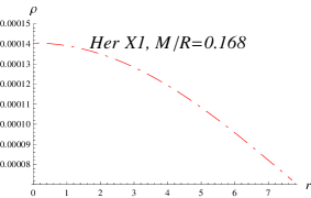
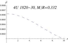
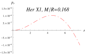
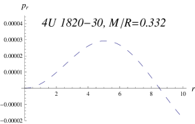
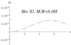
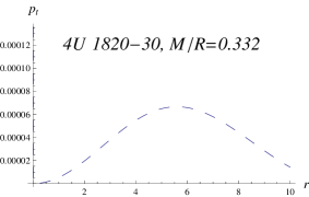
Here, we present the evolution of $\rho$, $p_{r}$ and $p_{t}$ as shown in Figs.1-3 for the strange star candidates Her X-1, SAX J 1808.4-3658 and 4U 1820-30 (see table 1). Herein, we set $n=2$ and $\beta=-2$.

Figure 1: Evolution of energy density $\rho$ versus radial coordinate $r(km)$ at the stellar interior of strange star candidates.

Figure 2: Evolution of radial pressure $p_{r}$ versus radial coordinate $r(km)$ at the stellar interior of strange star candidates.

Figure 3: Evolution of tangential pressure $p_{t}$ versus radial coordinate $r(km)$ at the stellar interior of strange star candidates.

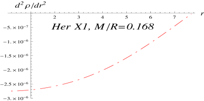
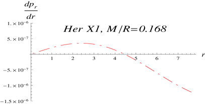
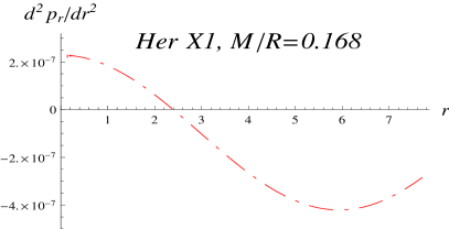
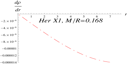
From Eqs.(15) and (16), one can find the expressions for $d\rho/dr$, $d^{2}\rho/dr^{2}$, $dp_{r}/dr$ and $d^{2}\rho/dr^{2}$. We show the results for $d\rho/dr$ and $dp_{r}/dr$ in Appendix as Eqs.(A.1) and (A.2) respectively. Figures 4 and 5 show the variation of derivatives of $\rho$ and $p_{r}$ with respect to radial coordinate for strange star Her X1. We find that $d\rho/dr<0$ and $dp_{r}/dr$ shows transition from positive to negative values.

Figure 4: Evolution of $d\rho/dr$ and $d^{2}\rho/dr^{2}$ versus $r(km)$ at the stellar interior of Her X1.

Figure 5: Evolution of $dp_{r}/dr$ and $d^{2}p_{r}/dr^{2}$ versus $r(km)$ at the stellar interior of Her X1.

We also examine behavior of derivatives at $r=0$, centre of strange star Her X1. It can be seen that

$$\frac{d\rho}{dr}=0,\quad\quad\frac{dp_{r}}{dr}=0,$$

$$\frac{d^{2}\rho}{dr^{2}}<0,\quad\quad\frac{d^{2}p_{r}}{dr^{2}}>0.$$ (20)

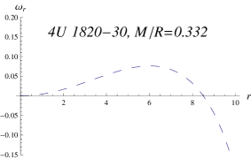
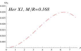
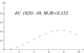
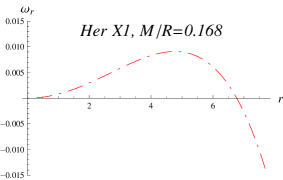
Clearly, at $r=0$, density is maximum and it decreases outward with the increase in $r$ as shown in Figure 1. In case of $p_{r}$, we have increasing function unlike the evolution $\rho$, which attains maximum value in midway to the boundary of star and then decreases. One can test the evolution of $\rho$ and $p_{r}$ for the strange stars SAX J 1808.4-3658 and 4U 1820-30, which would show similar behavior. The evolution of EoS parameters $\omega_{r}$ and $\omega_{t}$ is also presented for the strange stars in $f(T)$ gravity. It can be seen that $\omega_{r}>0$, which favors the quintessence regime near the boundary of star whereas $0<\omega_{t}<1$ despite of the role of modified gravity.

Figure 6: Evolution of $\omega_{r}$ versus radial coordinate $r(km)$ at the stellar interior of strange star candidates.

Figure 7: Evolution of radial pressure $\omega_{t}$ versus radial coordinate $r(km)$ at the stellar interior of strange star candidates.

The anisotropy measurement in $f(T)$ gravity, for spherically symmetric metric is given by

$$\Delta = \frac{2(p_{t}-p_{r})}{r}=\frac{n2^{n-1}\beta}{r^{2n+1}}\left\{(e^{-Ar^{2}})^{n}\left(\left(e^{\frac{Ar^{2}}{2}}-1\right)\left(e^{\frac{Ar^{2}}{2}}-1-2Br^{2}\right)\right)^{n-2}\right\}$$ (21)

$$\times \left[e^{2Ar^{2}}+2e^{\frac{3Ar^{2}}{2}}(-2+n-Br^{2})+e^{Ar^{2}}(6+Ar^{2}+4Br^{2}+ABr^{4}\right.$$

$$\left.+B^{2}r^{4}-2n(3+Ar^{2}+Br^{2}+ABr^{4}))+(1+Br^{2})(1+Ar^{2}-Br^{2}\right.$$

$$\left.+2ABr^{4}+2B^{2}r^{4}-2n(1+Ar^{2}+2ABr^{4}))+2e^{\frac{Ar^{2}}{2}}(-2-Ar^{2}-Br^{2}\right.$$

$$\left.-2ABr^{4}-B^{2}r^{4}-B^{3}r^{6}+n(3+2Br^{2}+Ar^{2}(2+4Br^{2}+B^{2}r^{4})))\right].$$

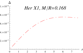
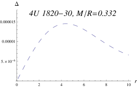
The measure of anisotropy depends on radial and tangential pressures, it is directed outward when $p_{t}>p_{r}$ which implies $\Delta>0$ whereas $p_{t}<p_{r}$ results in $\Delta<0$ so that anisotropy is directed inward. We present the evolution of $\Delta$ for strange star candidates Her X-1, SAX J 1808.4-3658 and 4U 1820-30 in Fig. 8. It can be seen that $\Delta>0$ for our model which implies the existence of repulsive force, allowing more massive distribution. One can see that $f(T)$ gravity does not affect the anisotropic force. Here, $\Delta$ vanishes at the center $r=0$.

Figure 8: Evolution of anisotropy measurement $\Delta$ versus radial coordinate $r(km)$ at the stellar interior of strange star candidates.

3.2 Matching Conditions

Here, we match the interior metric (7) to the vacuum exterior spherically symmetric metric given by

$$ds^{2}=-\left(1-\frac{2M}{r}\right)dt^{2}+\left(1-\frac{2M}{r}\right)^{-1}dr^{2}+r^{2}d\theta^{2}+r^{2}Sin^{2}\theta{d}\varphi^{2},$$ (22)

At the boundary surface $r=R$ continuity of the metric functions $g_{tt}$, $g_{rr}$ and $\frac{\partial g_{tt}}{\partial r}$ yield,

$$g_{tt}^{-}=g_{tt}^{+},~{}~{}~{}~{}~{}g_{rr}^{-}=g_{rr}^{+},~{}~{}~{}~{}~{}\frac{\partial g_{tt}^{-}}{\partial r}=\frac{\partial g_{tt}^{+}}{\partial r},$$ (23)

where $-$ and $+$, correspond to interior and exterior solutions. From the interior and exterior metrics, we get

$$A = -\frac{1}{R^{2}}ln\left(1-\frac{2M}{R}\right),$$ (24)

$$B = \frac{M}{R^{3}}{{\left(1-\frac{2M}{R}\right)}^{-1}},$$ (25)

$$C = ln\left(1-\frac{2M}{R}\right)-\frac{M}{R}{{\left(1-\frac{2M}{R}\right)}^{-1}}.$$ (26)

For the given values of $M$ and $R$ for given star, the constants $A$ and $B$ takes the values as given in the table 1.

Table 1: Values of constants for given Masses and Radii of Stars [35, 36]

Strange Quark Star	$M$	$R(km)$	$\frac{M}{R}$	$A(km^{-2})$	$B(km^{-2})$
Her X-1	0.88$M_{\odot}$	7.7	0.168	0.006906276428	$0.004267364618$
SAX J 1808.4-3658	1.435$M_{\odot}$	7.07	0.299	0.01823156974	$0.01488011569$
4U 1820-30	2.25$M_{\odot}$	10.0	0.332	0.01090644119	$0.009880952381$

3.3 Energy Conditions

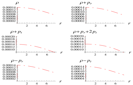
Energy conditions have been a handy tool to limit the arbitrariness in the energy-momentum tensor, based on Raychaudhuri equation with attractiveness property of gravity. These conditions include weak energy condition (WEC), null energy condition (NEC), strong energy condition (SEC) and dominant energy condition (DEC). In case of anisotropic fluid, we find the following inequalities

$$\textbf{NEC}:\quad \rho+p_{r}\geq 0,\quad\rho+p_{t}\geq 0,$$

$$\textbf{WEC}:\quad \rho\geq 0,\quad\rho+p_{r}\geq 0,\quad\rho+p_{t}\geq 0,$$

$$\textbf{SEC}:\quad \rho+p_{r}\geq 0,\quad\rho+p_{t}\geq 0,\quad\rho+p_{r}+2p_{t}\geq 0,$$

$$\textbf{DEC}:\quad \rho>|p_{r}|,\quad\rho>|p_{t}|.$$

We examine these constraints for the strange star Her X-1 and show the evolution in Figure 9. It can be seen that these conditions are satisfied for strange star Her X-1 and one can also the constraints on other strange star models.

Figure 9: Evolution of energy constraints at the stellar interior of strange star Her X-1.

3.4 TOV Equation

For an anisotropic fluid the generalized Tolman-Oppenheimer-Volkoff (TOV) equation has the following form

$$\frac{dp_{r}}{dr}+\frac{\nu^{\prime}(\rho+p_{r})}{2}+\frac{2(p_{r}-p_{t})}{r}=0.$$ (27)

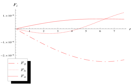
Following [37], we can express the above equation in terms of gravitational mass and henceforth it results in the equilibrium condition for the strange star, involving the gravitational, hydrostatic and anisotropic forces of the stellar object as

$$F_{g}+F_{h}+F_{a}=0,$$

$$F_{g}=-Br(\rho+p_{r}),\quad F_{h}=-\frac{dp_{r}}{dR},\quad F_{a}=\frac{2(p_{t}-p_{r})}{r}.$$ (28)

Using the effective $\rho$, $p_{r}$ and $p_{t}$ (10)-(12), we can find the numerically the equilibrium condition in $f(T)$ theory. In Figure 10, we show the evolution of above forces at the interior of strange star Her X-1. This figure indicates that the static equilibrium can be attained due to pressure anisotropy, gravitational and hydrostatic forces for strange star candidates in $f(T)$ gravity.

Figure 10: Evolution of gravitating, hydrostatic and pressure anisotropic forces at the stellar interior of strange star Her X-1.

3.5 Stability Analysis

In this section, we discuss the stability of strange star models in $f(T)$ theory. The radial and transverse speeds can be calculated as

$$v_{sr}^{2}=\left[(-1+e^{\frac{Ar^{2}}{2}}-2Br^{2})(e^{2Ar^{2}}+2e^{\frac{3Ar^{2}}{2}}(n-2)(1+Br^{2})-(2n-1)(1\right.$$

$$\left.+2Br^{2})(1+A(r^{2}+2Br^{4}))+e^{(}Ar^{2})(6+10Br^{2}+A(r^{2}+2Br^{4}+2B^{2}r^{6})\right.$$

$$\left.-2n(3+4Br^{2}+A(r+Br^{3})^{2}))+2e^{\frac{Ar^{2}}{2}}(-(1+2Br^{2})(2+A(r^{2}+Br^{4}))\right.$$

$$\left.+n(3+5Br^{2}+2A(3Br^{4}+r^{2}+2B^{2}r^{6}))))\right]/\left[1-e^{\frac{5Ar^{2}}{2}}+7Ar^{2}-10Br^{2}\right.$$

$$\left.+18ABr^{4}+8B^{2}r^{4}+12AB^{2}r^{6}+8AB^{3}r^{8}+e^{2Ar^{2}}(5+4n^{2}-2Ar^{2}+6Br^{2}\right.$$

$$\left.+2n(-3+Ar^{2}-Br^{2}))+4n^{2}(1+A(r^{2}+2Br^{4}))^{2}-2n(2-7Br^{2}+2B^{2}r^{4}\right.$$

$$\left.+3r^{4}(A+2ABr^{2})^{2}+Ar^{2}(7+15Br^{2}+4B^{2}r^{4}+4B^{3}r^{6}))-e^{\frac{3Ar^{2}}{2}}(10+4Br^{2}\right.$$

$$\left.+8B^{2}r^{4}-2A^{2}r^{4}(3+2Br^{2})+Ar^{2}(16Br^{2}+2B^{2}r^{4}+3)+8n^{2}(2+A(r^{2}\right.$$

$$\left.+Br^{4}))+2n(-11+2Br^{2}-2B^{2}r^{4}-Ar^{2}(5+12Br^{2}+B^{2}r^{4})+2A^{2}(r^{4}\right.$$

$$\left.+Br^{6})))+e^{Ar^{2}}(-4A^{2}r^{4}(3+5Br^{2})+2(5-10Br^{2}+8B^{2}r^{4})+Ar^{2}(19\right.$$

$$\left.+56Br^{2}+16B^{2}r^{4}+4B^{3}r^{6})+4n^{2}(6+r^{4}(A+ABr^{2})^{2}+A(6r^{2}+8Br^{4}))\right.$$

$$\left.-2n(15-14Br^{2}+6B^{2}r^{4}+A^{2}r^{4}(-1-2Br^{2}+2B^{2}r^{4})+2Ar^{2}(21Br^{2}\right.$$

$$\left.+4B^{2}r^{4}+B^{3}r^{6}+10)))+e^{\frac{Ar^{2}}{2}}(-5+28Br^{2}-16B^{2}r^{4}+2A^{2}r^{4}(3+8Br^{2}\right.$$

$$\left.+4B^{2}r^{4})-Ar^{2}(21+58Br^{2}+30B^{2}r^{4}+12B^{3}r^{6})-8n^{2}(2+Ar^{2}(3+5Br^{2})\right.$$

$$\left.+A^{2}(r^{4}+3Br^{6}+2B^{2}r^{8}))+2n(9-18Br^{2}+6B^{2}r^{4}+Ar^{2}(21+45Br^{2}\right.$$

$$\left.+13B^{2}r^{4}+6B^{3}r^{6})+4A^{2}(r^{4}+3Br^{6}+2B^{2}r^{8})))\right].$$ (29)

$$v_{st}^{2}=-(-1+e^{\frac{3Ar^{2}}{2}}(n-1)-2Ar^{2}-10ABr^{4}-6B^{2}r^{4}-18AB^{2}r^{6}-6B^{3}r^{6}$$

$$-12AB^{3}r^{8}-4B^{4}r^{8}+e^{\frac{5Ar^{2}}{2}}(n-1)(-6+2n-Br^{2}(4+Ar^{2}))-2n^{2}(1$$

$$+Br^{2})(1+A(r^{2}+2Br^{4}))^{2}+n(3+2Br^{2}+5B^{2}r^{4}+2B^{3}r^{6}+r^{4}(1+Br^{2})$$

$$\times(A+2ABr^{2})^{2}+Ar^{2}(6+25Br^{2}+39B^{2}r^{4}+28B^{3}r^{6}+4B^{4}r^{8}))-e^{2Ar^{2}}(15$$

$$+16Br^{2}+6B^{2}r^{4}+Ar^{2}(2+10Br^{2}+3B^{2}r^{4})-A^{2}(r^{4}+Br^{6})+2n^{2}(5+Br^{2}$$

$$+2A(r^{2}+Br^{4}))+n(-25-18Br^{2}-5B^{2}r^{4}-Ar^{2}(6+17Br^{2}+4B^{2}r^{4})+2A^{2}(r^{4}$$

$$+Br^{6})))+e^{\frac{3Ar^{2}}{2}}(20+24Br^{2}+24B^{2}r^{4}+6B^{3}r^{6}-3A^{2}(r^{4}+2Br^{6})+Ar^{2}(34Br^{2}$$

$$+8+15B^{2}r^{4}+B^{3}r^{6})+2n^{2}(10+4Br^{2}+r^{4}(A+ABr^{2})^{2}+2Ar^{2}(6Br^{2}+B^{2}r^{4}$$

$$+4))+n(A^{2}r^{4}(5+10Br^{2}+2B^{2}r^{4})-2(20+16Br^{2}+10B^{2}r^{4}+B^{3}r^{6})-Ar^{2}(24$$

$$+70Br^{2}+35B^{2}r^{4}+5B^{3}r^{6})))-e^{Ar^{2}}(15+16Br^{2}+36B^{2}r^{4}+18B^{3}r^{6}+4B^{4}r^{8}$$

$$-3A^{2}(r^{4}+3Br^{6}+2B^{2}r^{8})+Ar^{2}(12+52Br^{2}+39B^{2}r^{4}+6B^{3}r^{6}-2B^{4}r^{8})$$

$$+2n^{2}(10+6Br^{2}+4Ar^{2}(3+6Br^{2}+2B^{2}r^{4})+A^{2}r^{4}(3+9Br^{2}+7B^{2}r^{4}+B^{3}r^{6}))+$$

$$n(-35-28Br^{2}-30B^{2}r^{4}-6B^{3}r^{6}+A^{2}r^{4}(3+9Br^{2}+8B^{2}r^{4}+2B^{3}r^{6})-Ar^{2}(36$$

$$+118Br^{2}+97B^{2}r^{4}+30B^{3}r^{6}+2B^{4}r^{8})))+e^{\frac{Ar^{2}}{2}}(6+4Br^{2}+24B^{2}r^{4}+18B^{3}r^{6}$$

$$+8B^{4}r^{8}+Ar^{2}(8+37Br^{2}+45B^{2}r^{4}+17B^{3}r^{6}-2B^{4}r^{8})-A^{2}(r^{4}+4Br^{6}+6B^{2}r^{8}$$

$$+4B^{3}r^{1}0)+2n^{2}(5+4Br^{2}+2Ar^{2}(4+10Br^{2}+5B^{2}r^{4})+A^{2}r^{4}(12Br^{2}+14B^{2}r^{4}$$

$$+3+4B^{3}r^{6}))+n(-2(8+6Br^{2}+10B^{2}r^{4}+3B^{3}r^{6})+A^{2}r^{4}(-1-4Br^{2}-2B^{2}r^{4}$$

$$+4B^{3}r^{6})-Ar^{2}(24+89Br^{2}+105B^{2}r^{4}+53B^{3}r^{6}+6B^{4}r^{8}))))/((-1+e^{\frac{Ar^{2}}{2}}(1$$

$$-e^{\frac{5Ar^{2}}{2}}+7Ar^{2}-10Br^{2}+18ABr^{4}+8B^{2}r^{4}+12AB^{2}r^{6}+8AB^{3}r^{8}+e^{2Ar^{2}}(5+4n^{2}$$

$$-2Ar^{2}+6Br^{2}+2n(-3+Ar^{2}-Br^{2}))+4n^{2}(1+A(r^{2}+2Br^{4}))^{2}-2n(2-7Br^{2}$$

$$+2B^{2}r^{4}+3r^{4}(A+2ABr^{2})^{2}+Ar^{2}(7+15Br^{2}+4B^{2}r^{4}+4B^{3}r^{6}))-e^{\frac{3Ar^{2}}{2}}(10$$

$$+4Br^{2}+8B^{2}r^{4}-2A^{2}r^{4}(3+2Br^{2})+Ar^{2}(3+16Br^{2}+2B^{2}r^{4})+8n^{2}(2+A(r^{2}$$

$$+Br^{4}))+2n(-11+2Br^{2}-2B^{2}r^{4}-Ar^{2}(5+12Br^{2}+B^{2}r^{4})+2A^{2}(r^{4}+Br^{6})))$$

$$+e^{Ar^{2}}(-4A^{2}r^{4}(3+5Br^{2})+2(5-10Br^{2}+8B^{2}r^{4})+Ar^{2}(19+56Br^{2}+16B^{2}r^{4}$$

$$+4B^{3}r^{6})+4n^{2}(6+r^{4}(A+ABr^{2})^{2}+A(6r^{2}+8Br^{4}))-2n(15-14Br^{2}+6B^{2}r^{4}$$

$$+A^{2}r^{4}(-1-2Br^{2}+2B^{2}r^{4})+2Ar^{2}(10+21Br^{2}+4B^{2}r^{4}+B^{3}r^{6})))+e^{\frac{Ar^{2}}{2}}(-5$$

$$+28Br^{2}-16B^{2}r^{4}+2A^{2}r^{4}(3+8Br^{2}+4B^{2}r^{4})-Ar^{2}(21+58Br^{2}+30B^{2}r^{4}$$

$$+12B^{3}r^{6})-8n^{2}(2+Ar^{2}(3+5Br^{2})+A^{2}(r^{4}+3Br^{6}+2B^{2}r^{8}))+2n(9-18Br^{2}$$

$$+6B^{2}r^{4}+Ar^{2}(21+45Br^{2}+13B^{2}r^{4}+6B^{3}r^{6})+4A^{2}(r^{4}+3Br^{6}+2B^{2}r^{8}))))).$$ (30)

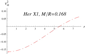
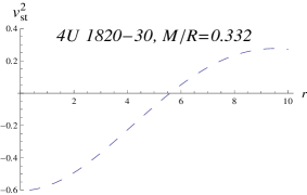
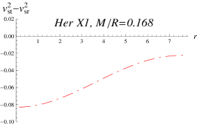
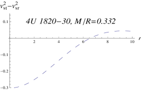
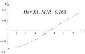
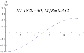
In [38], Herrera developed a new technique to explore the potentially unstable matter configuration and introduced the concept of cracking. One can analyze the potentially stable and unstable regions regions depending on the difference of sound speeds, the region for which radial sound speed is greater than the transverse sound speed is said to be potentially stable. In Figure 11 and 12, we plot the radial and transverse speeds for different strange star candidates. Here, the values of $v^{2}_{sr}$ and $v^{2}_{st}$ lies in the range $0<|v^{2}_{i}|<1$ within the anisotropic matter configuration. We also present the evolution of $v^{2}_{st}-v^{2}_{sr}$ in Figure 13, which shows that difference of two sound speeds satisfies the inequality $|v^{2}_{st}-v^{2}_{sr}|\leq 1$. Moreover, $v^{2}_{st}-v^{2}_{sr}$ retain the similar sign for Her X-1 whereas the sign changes in case of SAX J 1808.4-3658 and 4U 1820-30. Hence, our proposed strange star model is stable for Her X-1 and unstable for both SAX J 1808.4-3658 and 4U 1820-30.

Figure 11: Evolution of $v^{2}_{sr}$ versus radial coordinate $r(km)$ at the stellar interior of strange star candidates.

Figure 12: Evolution of $v^{2}_{st}$ versus radial coordinate $r(km)$ at the stellar interior of strange star candidates.

Figure 13: Evolution of $v^{2}_{st}-v^{2}_{sr}$ versus radial coordinate $r(km)$ at the stellar interior of strange star candidates.

3.6 Surface Redshift

The compactness of star in $f(T)$ gravity can be found as

$$u=\frac{M}{b}=\frac{e^{-2AR^{2}}\pi R\beta}{9(AR^{2})^{\frac{3}{2}}}\left[-36(20A^{2}+2AB+B^{2})e^{2AR^{2}}\sqrt{\pi}R^{2}Erf[\sqrt{AR^{2}}]\right.$$

$$\left.+16(24A^{2}+AB+B^{2})e^{2AR^{2}}Sqrt{6\pi}R^{2}Erf[\sqrt{\frac{3}{2}}\sqrt{AR^{2}}]-3(4\sqrt{AR^{2}}(-B^{2}\right.$$

$$\left.(3-8e^{\frac{AR^{2}}{2}}+6e^{AR^{2}})R^{2}+A(27-24e^{\frac{3AR^{2}}{2}}+3e^{2AR^{2}}+6BR^{2}-8e^{\frac{AR^{2}}{2}}(9\right.$$

$$\left.+2BR^{2})+6e^{AR^{2}}(11+2BR^{2})))-48A^{2}e^{2AR^{2}}\sqrt{2\pi}R^{2}Erf[\frac{\sqrt{AR^{2}}}{\sqrt{2}}]+3(32A^{2}\right.$$

$$\left.-2AB+B^{2})e^{2AR^{2}}\sqrt{2\pi}R^{2}Erf[\sqrt{2}\sqrt{AR^{2}}])\right].$$ (31)

The surface redshift corresponding to compactness is given by

$$1+Z_{s}=(1-2u)^{-1/2}=\{1-\frac{2e^{-2AR^{2}}\pi R\beta}{9(AR^{2})^{\frac{3}{2}}}\left[-36(20A^{2}+2AB+B^{2})e^{2AR^{2}}\right.$$

$$\left.\sqrt{\pi}R^{2}Erf[\sqrt{AR^{2}}]+16(24A^{2}+AB+B^{2})e^{2AR^{2}}\sqrt{6\pi}R^{2}Erf[\sqrt{\frac{3}{2}}\sqrt{AR^{2}}]\right.$$

$$\left.-3(4\sqrt{AR^{2}}(-B^{2}(3-8e^{\frac{AR^{2}}{2}}+6e^{AR^{2}})R^{2}+A(27-24e^{\frac{3AR^{2}}{2}}+3e^{2AR^{2}}+6BR^{2}\right.$$

$$\left.-8e^{\frac{AR^{2}}{2}}(9+2BR^{2})+6e^{AR^{2}}(11+2BR^{2})))-48A^{2}e^{2AR^{2}}\sqrt{2\pi}R^{2}Erf[\frac{\sqrt{AR^{2}}}{\sqrt{2}}]\right.$$

$$\left.+3(32A^{2}-2AB+B^{2})e^{2AR^{2}}\sqrt{2\pi}R^{2}Erf[\sqrt{2}\sqrt{AR^{2}}])\right]\}.$$ (32)

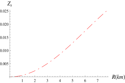
In Figure 13, we show the redshift plot for the star Her X-1 and maximum redshift turns out to be $Z_{s}=0.025$.

Figure 14: Evolution reshift $Z_{s}$ versus radial coordinate $r(km)$ at the stellar interior of strange star Her X-1.

4 Conclusion

In this paper, we have addressed the issue of modeling the spherically anisotropic compact stars in $f(T)$ gravity using the off diagonal tetrad field. For the analytic solution of the system of differential equations, we have assumed the KB form of the metyric components and the power law form of $f(T)$ model, as $f(T)=\beta T^{n}$, with $n\neq 1$ and $\beta$ is an arbitrary small constant, which plays the role of departure of these theories from GR. This approach leads to the set field equations, which second order nonlinear differential equations, for the analytic form of solutions we assume that the metric coefficients for the interior and exterior regions of a star continuous over the boundary. This is the smooth matching of the general spherical interior geometry with the Schwarzschild exterior geometry, because in both regions metric function are continuous upto fist order of derivatives (GR and $f(T)$ are second order derivative theories). This matching helps to use the observational data of stars for the calculation of arbitrary constants appearing in the system due to parameterization of metric functions.

We have determined the explicit form of the matter density and pressure components, which are regular inside the stars as shown in figures (1-3). The behavior of EoS parameter implies that near the boundary the matter inside the stars behaves as quintessence in the presence of $f(T)$ terms (see figure 6). The anisotropic parameter $\Delta=0$ at center vanished and it becomes $\Delta>0$, everywhere inside the star except at center, which predicts that there may exist the repulsive force which leads to the formation of more massive star. The physical viability of the solutions lies in the fact that solutions satisfies the energy conditions (Figure 9). The analysis of TOV equation presented in this paper shows that the static equilibrium can be achieved for strange stars in $f(T)$ as shown in figure 10. The stability of the proposed model is given in figures 11-13, on the physical investigations of these figures predict that our proposed strange star model is stable for Her X-1, and unstable for both SAX J 1808.4-3658 and 4U 1820-30. The maximum redshift of Her X-1 turn out be 0.025 which is shown in Figure 14.

Appendix A

$$\frac{\partial\rho}{\partial r}=\frac{n2^{n-1}\beta}{r^{2n+1}}\left\{(e^{-Ar^{2}})^{n}\left(e^{\frac{Ar^{2}}{2}}-1\right)^{n-2}\left(e^{\frac{Ar^{2}}{2}}-1-2Br^{2}\right)^{n-3}\right\}\left[7Ar^{2}-e^{\frac{5Ar^{2}}{2}}\right.$$

$$\left.+1-10Br^{2}+18ABr^{4}+12AB^{2}r^{6}+8AB^{3}r^{8}+e^{2Ar^{2}}(5+4n^{2}-2Ar^{2}+6Br^{2}\right.$$

$$\left.+2n(-3+Ar^{2}-Br^{2}))+4n^{2}(1+A(r^{2}+2Br^{4}))^{2}-2n(2B^{2}r^{4}-7Br^{2}+2\right.$$

$$\left.+3A^{2}r^{4}(1+2Br^{2})^{2}+Ar^{2}(7+15Br^{2}+4B^{2}r^{4}+4B^{3}r^{6}))-e^{\frac{3Ar^{2}}{2}}(10+4Br^{2}\right.$$

$$\left.+8B^{2}r^{4}-2A^{2}r^{4}(3+2Br^{2})+Ar^{2}(3+16Br^{2}+2B^{2}r^{4})+8n^{2}(2+A(r^{2}+Br^{4}))\right.$$

$$\left.+2n(2Br^{2}-11-2B^{2}r^{4})-Ar^{2}(5+12Br^{2}+B^{2}r^{4})+2A^{2}r^{4}(1+Br^{2})))+e^{Ar^{2}}\right.$$

$$\left.\times(10-20Br^{2}+16B^{2}r^{4}-4A^{2}r^{4}(3+5Br^{2})+Ar^{2}(56Br^{2}+16B^{2}r^{4}+4B^{3}r^{6}\right.$$

$$\left.+19)+4n^{2}(6+r^{4}(A+ABr^{2})^{2}+A(6r^{2}+8Br^{4}))-2n(15-14Br^{2}+6B^{2}r^{4}\right.$$

$$\left.+A^{2}r^{4}(-1-2Br^{2}+2B^{2}r^{4})+2Ar^{2}(10+21Br^{2}+4B^{2}r^{4}+B^{3}r^{6})))+e^{\frac{Ar^{2}}{2}}(-5\right.$$

$$\left.+28Br^{2}-16B^{2}r^{4}+2A^{2}r^{4}(3+8Br^{2}+4B^{2}r^{4})-Ar^{2}(58Br^{2}+30B^{2}r^{4}+12B^{3}r^{6}\right.$$

$$\left.+21)-8n^{2}(2+Ar^{2}(3+5Br^{2})+A^{2}(r^{4}+3Br^{6}+2B^{2}r^{8}))+2n(-18Br^{2}+9+\right.$$

$$\left.6B^{2}r^{4}+Ar^{2}(21+45Br^{2}+13B^{2}r^{4}+6B^{3}r^{6})+4A^{2}(r^{4}+3Br^{6}+2B^{2}r^{8})))\right],$$ (A.1)

$$\frac{\partial p_{r}}{\partial r}=\frac{n2^{n-1}\beta}{r^{2n+1}}\left\{(e^{-Ar^{2}})^{n}(\left(e^{\frac{Ar^{2}}{2}}-1\right)\left(e^{\frac{Ar^{2}}{2}}-1-2Br^{2}\right))^{n-2}\right\}\left[2e^{\frac{3Ar^{2}}{2}}(-2+n)\right.$$ (A.2)

$$\times \left.(1+Br^{2})+e^{2Ar^{2}}-(2n-1)(1+2Br^{2})(1+A(r^{2}+2Br^{4}))+e^{Ar^{2}}(6+10Br^{2}\right.$$

$$+ \left.A(r^{2}+2Br^{4}+2B^{2}r^{6})-2n(3+4Br^{2}+A(r+Br^{3})^{2}))+2e^{\frac{Ar^{2}}{2}}(-(1+2Br^{2})(2\right.$$

$$+ \left.A(r^{2}+Br^{4}))+n(3+5Br^{2}+2A(r^{2}+3Br^{4}+2B^{2}r^{6})))\right],$$

$$\frac{\partial p_{t}}{\partial r}=\frac{-n2^{n-1}\beta}{r^{2n+1}}\left\{(e^{-Ar^{2}})^{n}(\left(e^{\frac{Ar^{2}}{2}}-1\right)\left(e^{\frac{Ar^{2}}{2}}-1-2Br^{2}\right))^{n-3}\right\}\left[e^{3Ar^{2}}(n-1)-1\right.$$

$$\left.-2Ar^{2}-10ABr^{4}-6B^{2}r^{4}-18AB^{2}r^{6}-6B^{3}r^{6}-12AB^{3}r^{8}-4B^{4}r^{8}+e^{\frac{5Ar^{2}}{2}}(n-1)\right.$$

$$\left.\times(2n-6-Br^{2}(4+Ar^{2}))-2n^{2}(1+Br^{2})(1+A(r^{2}+2Br^{4}))^{2}+n(2Br^{2}+5B^{2}r^{4}\right.$$

$$\left.+3+2B^{3}r^{6}+r^{4}(1+Br^{2})(A+2ABr^{2})^{2}+Ar^{2}(6+25Br^{2}+39B^{2}r^{4}+28B^{3}r^{6}\right.$$

$$\left.+4B^{4}r^{8}))-e^{2Ar^{2}}(15+16Br^{2}+6B^{2}r^{4}+Ar^{2}(2+10Br^{2}+3B^{2}r^{4})-A^{2}r^{4}(1+Br^{2})\right.$$

$$\left.+2n^{2}(5+Br^{2}+2A(r^{2}+Br^{4}))+n(-25-18Br^{2}-5B^{2}r^{4}-Ar^{2}(17Br^{2}+4B^{2}r^{4}\right.$$

$$\left.+6)+2A^{2}(r^{4}+Br^{6})))+e^{\frac{3Ar^{2}}{2}}(20+24Br^{2}+24B^{2}r^{4}+6B^{3}r^{6}-3A^{2}(r^{4}+2Br^{6})\right.$$

$$\left.+Ar^{2}(8+34Br^{2}+15B^{2}r^{4}+B^{3}r^{6})+2n^{2}(10+4Br^{2}+r^{4}(A+ABr^{2})^{2}+2Ar^{2}(4\right.$$

$$\left.+6Br^{2}+B^{2}r^{4}))+n(A^{2}r^{4}(5+10Br^{2}+2B^{2}r^{4})-2(20+16Br^{2}+10B^{2}r^{4}+B^{3}r^{6})\right.$$

$$\left.-Ar^{2}(24+70Br^{2}+35B^{2}r^{4}+5B^{3}r^{6})))-e^{Ar^{2}}(16Br^{2}+36B^{2}r^{4}+18B^{3}r^{6}+4B^{4}r^{8}\right.$$

$$\left.+15-3A^{2}(r^{4}+3Br^{6}+2B^{2}r^{8})+Ar^{2}(12+52Br^{2}+39B^{2}r^{4}+6B^{3}r^{6}-2B^{4}r^{8})\right.$$

$$\left.+2n^{2}(10+6Br^{2}+4Ar^{2}(3+6Br^{2}+2B^{2}r^{4})+A^{2}r^{4}(3+9Br^{2}+7B^{2}r^{4}+B^{3}r^{6}))\right.$$

$$\left.+n(-35-28Br^{2}-30B^{2}r^{4}-6B^{3}r^{6}+A^{2}r^{4}(3+9Br^{2}+8B^{2}r^{4}+2B^{3}r^{6})-Ar^{2}(36\right.$$

$$\left.+118Br^{2}+97B^{2}r^{4}+30B^{3}r^{6}+2B^{4}r^{8})))+e^{\frac{Ar^{2}}{2}}(4Br^{2}+24B^{2}r^{4}+18B^{3}r^{6}+8B^{4}r^{8}\right.$$

$$\left.+6+Ar^{2}(8+37Br^{2}+45B^{2}r^{4}+17B^{3}r^{6}-2B^{4}r^{8})-A^{2}r^{4}(4Br^{2}+6B^{2}r^{4}+4B^{3}r^{6}\right.$$

$$\left.+1)+2n^{2}(5+4Br^{2}+2Ar^{2}(4+10Br^{2}+5B^{2}r^{4})+A^{2}r^{4}(12Br^{2}+14B^{2}r^{4}+4B^{3}r^{6}\right.$$

$$\left.+3))+n(-2(8+6Br^{2}+10B^{2}r^{4}+3B^{3}r^{6})+A^{2}r^{4}(-1-4Br^{2}-2B^{2}r^{4}+4B^{3}r^{6})\right.$$

$$\left.-Ar^{2}(24+89Br^{2}+105B^{2}r^{4}+53B^{3}r^{6}+6B^{4}r^{8})))\right]$$ (A.3)

References

• [1] A. G. Riess et al. [Supernova Search Team Collaboration], Astron. J. 116, 1009 (1998).
• [2] S. Perlmutter et al. [Supernova Cosmology Project Collaboration], Astrophys. J. 517, 565 (1999).
• [3] G. Hinshaw et al. [WMAP Collaboration], Astrophys. J. Suppl. 208, 19 (2013)
• [4] D. J. Eisenstein et al. [SDSS Collaboration], Astrophys. J. 633, 560 (2005) .
• [5] Y. Wang, Phys. Rev. D 78, 123532 (2008).
• [6] J. Binney, ,S. Tremaine, Galactic Dynamics, Princeton University Press, Princeton (1987)
• [7] T. P. Sotiriou and V. Faraoni, Rev. Mod. Phys. 82, 451 (2010)
• [8] Bamba, K. Capozziello, S. Nojiri, S. and Odintsov, S.D., Astrophys. Space Sci. 345 ,155 (2012).
• [9] R. Aldrovandi and J. G. Pereira, Teleparallel Gravity: An Introduction, Springer Dordrecth, (2012).
• [10] A. Einstein, S.B. Preuss. Akad. Wiss. 22, 414-419 (1925).
• [11] R. Ferraro and F. Fiorini, Phys. Rev. D 78, 124019 (2008).
• [12] F. Fiorini and R. Ferraro, Int. J. Mod. Phys. A 24, 1686 (2009).
• [13] V.F. Cardone, N. Radicella, S. Camera, Phys. Rev. D 85, 124007 (2012)
• [14] M. Li, R. X. Miao and Y.G. Miao, JHEP 1107, 108 (2011).
• [15] B. Li, T. P. Sotiriou and J. D. Barrow, Phys. Rev. D 83, 064035 (2011).
• [16] N. Tamanini and C. G. Boehmer, Phys. Rev. D 86, 044009 (2012).
• [17] S. Camera, V. F. Cardone and N. Radicella, Phys. Rev. D 89, 083520 (2014).
• [18] C. M. Will, Living Rev. Rel. 9, 3 (2006).
• [19] L. Iorio and E. N. Saridakis, Mon. Not. Roy. Astron. Soc. 427,(2012)1555.
• [20] Y. Xie and X. M. Deng, Mon. Not. Roy. Astron. Soc. 433 (2013)3584.
• [21] J. B. Dent, S. Duuta and E.N. Saridakis, JCAP 1101, 009(2011).
• [22] M. Rong-Xin, M. Lie and Yan-Gang Miao, JCAP 11, 033(2011).
• [23] T. Wang Phys. Rev. D 84, 024042(2011).
• [24] C. G. Boehmer, A. Mussa and N. Tamani Class. Qunatum Gravity 28, 245020(2011).
• [25] M. H. Daouda, M. E. Rodrigues, M.J.S. Houndjo, EJPC 71, 1817(2011).
• [26] G. Abbas, S. Nazeer and M. A. Meraj, Astrophys. Space Science 354, 449(2014).
• [27] G. Abbas, A. Kanwal, and M. Zubair, Anisotropic Compact Stars in f​(T)𝑓𝑇f(T) gravity (Submitted).
• [28] M. Zubair, and G. Abbas, Anisotropic Compact Stars in f​(R)𝑓𝑅f(R) gravity (Submitted).
• [29] G. Abbas, et al. Anisotropic Compact Stars in f​(G)𝑓𝐺f(G) gravity (Submitted).
• [30] K. D. Krori and J. Barua, J. Phys. A.: Math. Gen. 8, 508(1975).
• [31] M.H., Daouda, M. E. Rodrigues, and M. J. S. Houndjo, Phys. Lett. B 715, 241(2012).
• [32] E. V. Linder, Phys. Rev. D 81, 127301(2010).
• [33] K. Bamba, et al, Phys. Rev. D 85, 104036 (2012)
• [34] M. R. Setare, and F. Darabi, Gen. Relativ. Gravit. DOI 10.1007/s10714-012-1408-6.
• [35] J.Β M. Lattimer Β and A. W. Steiner, Astrophys.Β J.Β  784, 123 (2014).
• [36] X. D. Li, I. Bombaci, M. Dey, J. DeyΒ  and E.Β P.Β J. van den Heuvel. Phys.Β Rev.Β Lett.Β  83, 3776 (1999).
• [37] S.K.M. Hossein et al. Int. J. Mod. Phys. D, 21, 1250088(2012).
• [38] L. Herrera, Phys. Lett. A, 165, 206(1992).