Unraveling the success and failure of mode coupling theory from consideration of entropy

Abstract

We analyze the dynamics of model supercooled liquids in a temperature regime where predictions of mode coupling theory (MCT) are known to be valid qualitatively. In this regime, the Adam-Gibbs (AG) relation, based on an activation picture of dynamics also describes the dynamics satisfactorily, and we explore the mutual consistency and interrelation of these descriptions. Although entropy and dynamics are related via phenomenological theories, the connection between MCT and entropy has not been argued for. In this work we explore this connection and provide a microscopic derivation of the phenomenological Rosenfeld theory. At low temperatures the overlap between MCT power law regime and AG relation implies that the AG relation predicts an avoided divergence at $T_{c}$, the origin of which is traced back to the vanishing of pair configurational entropy, which we find occurs at the same temperature. We also show that the residual multiparticle entropy plays an important role in describing the relaxation time.

I Introduction

In the study of liquid state physics, the structure of the liquid, which is often described primarily by the two body radial distribution function (rdf), has always played a central role. The structure can not only describe the thermodynamic properties of the liquid like the energy and pressure, under certain theoretical frameworks like the mode coupling theory the structure can also determine the dynamics sjogren ; Gotze . In a series of paper Berthier and Tarjus have described the behaviour of two systems with different interaction potentials, namely, the Lennard-Jones (LJ) and the Weeks-Chandler-Andersen (WCA) potentials. Although at the same temperature and density the structures of these systems are very close, the dynamics display significant differences at low temperatures tarjus_prl ; tarjus_pre ; tarjus_epje ; tarjus_berthier_jcp . These studies questioned the role of structure in determining the dynamics. Coslovich has shown that although the two body radial distribution function of these two systems are quite similar, triplet correlations are significantly different coslovich-jcp . He has also shown that the LJ system has more pronounced local ordering coslovich . In supercooled liquids these locally preferred structures are known to form correlated domains which have been argued to give rise to the slow dynamics tarjus . An estimation of this length scale of the domains and its connection to the relaxation timescale is a topic of ongoing research Smarajit_pre ; Paddy-jcp13 . One such study by Hocky et al. has shown that the point-to-set correlation length of the LJ system is larger compared to that of the WCA system and that this difference in correlation length can account for the difference in dynamics of the two systems hocky-prl . From these studies one may conclude that the difference in dynamics primarily comes from many body correlations. However, in a recent study by some of us it has been shown that two body correlation information is good enough to capture the difference in the dynamics between the two systems. The study also reveals that the divergence temperature at which an approximation to the configurational entropy using pair correlation alone goes to zero, is similar to the mode coupling theory (MCT) transition temperature, $T_{c}$ bssb . As mentioned before, MCT is a microscopic theory where the structural inputs determine the dynamics. Although entropy and dynamics are related via phenomenological Rosenfeld Rosenfeld and Adam-Gibbs (AG) adam-gibbs relations at high and low temperatures respectively, MCT does not have any apparent connection to entropy. Thus it is of great interest to try to understand the origin of the coincidence of the MCT divergence temperature and the temperature where pair configurational entropy goes to zero.

At normal liquid temperatures, a semi quantitative correlation between the dynamics (transport properties) and thermodynamics (excess entropy), proposed by Rosenfeld Rosenfeld ; Rosenfeld-iop , has been extensively studied in recent times, where the relaxation time $\tau$ can be written as,

$$\tau(T)=C\exp\left[-KS_{ex}\right]$$ (1)

Here $C$ and $K$ are the constants. Since the pair entropy $S_{2}$, which is obtained only from the pair correlation function, accounts for $80\%-90\%$ of the excess entropy Baranyai-cp ; bssb , many simulation studies have replaced $S_{ex}$ by $S_{2}$ and have shown that even with $S_{2}$ the transport coefficients follow Rosenfeld scaling tarjus_berthier_jcp ; Dzugutov ; hoyt ; trusket_2006 ; Ruchi_charu_2006 .

Bagchi and coworkers used Zwanzig’s rugged energy landscape model of diffusion zwanzig and by connecting the ruggedness to the excess entropy have provided a derivation of Rosenfeld relation saikat_jcp . Samanta et al alok have shown that under certain approximations the diffusion coefficient as obtained from MCT follows Rosenfeld scaling. Das and coworkers have performed microscopic MCT calculations which show that the diffusion values thus obtained can be fitted to Rosenfeld scaling shankar_das . Some of these studies have reported that the scaling parameter is not unique, hence the whole temperature region cannot be fitted to a single straight line shankar_das ; manish_charu .

Although Rosenfeld scaling holds at high temperature, it is known to breakdown at low temperatures even with multiple scaling parameters. At low temperatures the correlation between the transport coefficients and entropy is usually described by the well known Adam-Gibbs relation adam-gibbs ,

$$\tau(T)=\tau_{o}\exp\left(\frac{A}{TS_{c}}\right),$$ (2)

where $S_{c}$ is the configurational entropy of the system. For a wide range of systems, the AG relation is found to hold bssb ; shila-jcp ; shila-prl below a moderately high temperature referred to as the onset temperature of slow dynamics.

In this paper, we explore the connection between dynamics, characterization of structure as contained in the pair and higher order correlations, and entropy, and relations between them as described by MCT and the AG relation, using computer simulations of two model liquids and analytical results that seek to relate descriptions of dynamics in terms of structure, and entropy. Our present study shows that the AG theory, which is based on activation dynamics can completely describe the mode coupling theory (MCT) power law behavior in the region where the latter is found to be valid. An earlier study also observing similar overlap region sciortino-pre-2002 argued that the observation supports the hypothesis that a direct relation exists between the number of basins and their connectivity sciortino-prl-2000 ; sciortino-prl-2002 . In this work to understand the above mentioned observations, we explore the connection between mode coupling theory (MCT) and entropy and discuss different predictions of MCT in the light of entropy. We also analyze the different roles of pair and many body correlations.

Although MCT makes predictions about dynamics in both Rosenfeld and AG temperature regimes, no connection between MCT and entropy has been argued for, except for one study alok , as mentioned earlier. We show that, under some assumptions, the memory function in the MCT equation for structural relaxation is related to the pair excess entropy, thus providing a microscopic derivation of the phenomenological Rosenfeld expression for the structural relaxation time, $\tau$. Our study also can explain the origin of the temperature dependence of the Rosenfeld parameter. The origin of higher relaxation time and higher activation energy as predicted by MCT is also obtained from the analysis of the memory function.

As mentioned above the AG expression for relaxation times and the MCT power law form overlap in a certain temperature regime. The AG relation is valid for a wide temperature range which includes the range in which the MCT power law prediction holds. Thus in the MCT regime, the relaxation time follows both the AG and MCT behaviour. Our study reveals that the origin of the avoided divergence like behaviour (as given by MCT power law) in the AG relation is related to the vanishing of the pair configurational entropy. However we show that the pair configurational entropy, although predicting the correct MCT transition temperature, by itself cannot predict the MCT power law behaviour. The residual multiparticle entropy (RMPE) plays an important role in providing the correct temperature dependence of relaxation times. We also find a connection between the AG coefficient (A), pair thermodynamic fragility ($K_{T2}$) and MCT critical exponent ($\gamma$). We show that although both ‘A’ and $K_{T2}$ are dependent on density, their ratio which is related to $\gamma$ is density-independent.

The paper is organized as follows: The simulation details are given in Sec. II. In Sec. III we describe the methods used for evaluating the various quantities of interest and provide other necessary background. In Sec-IV we report some observations that motivate our analytical results which are described in Sec-V. In Sec-VI we present additional numerical results and their analysis. Sec. VII contains a discussion of presented results and conclusions.

II Simulation Details

We have performed molecular dynamics simulations of the Kob-Andersen model which is a binary mixture (80:20) of Lennard-Jones (LJ) particles and the corresponding WCA version kob ; chandler . The interatomic pair potential between species i and j, with ${\it i,j}=A,B$, $U_{ij}(r)$ is described by a shifted and truncated Lennard-Jones (LJ) potential, as given by:

$$U_{ij}(r)=\begin{cases}U_{ij}^{(LJ)}(r;\sigma_{ij},\epsilon_{ij})-U_{ij}^{(LJ)}(r^{(c)}_{ij};\sigma_{ij},\epsilon_{ij}),&r\leq r^{(c)}_{ij}\\ 0,&r>r^{(c)}_{ij}\end{cases}$$ (3)

where $U_{ij}^{(LJ)}(r;\sigma_{ij},\epsilon_{ij})=4\epsilon_{ij}[({\sigma_{ij}}/{r})^{12}-({\sigma_{ij}}/{r})^{6}]$ and $r^{(c)}_{ij}=2.5\sigma_{ij}$ for the LJ systems and $r^{(c)}_{ij}$ is equal to the position of the minimum of $U_{ij}^{(LJ)}$ for the WCA systems. Length, temperature and time are given in units of $\sigma_{11}$, ${k_{B}T}/{\epsilon_{11}}$ and $\tau=\surd({m_{1}\sigma_{11}^{2}}/{\epsilon_{11}})$, respectively. Here we have simulated Kob Andersen Model with the interaction parameters $\sigma_{11}$ = 1.0, $\sigma_{12}$ =0.8 ,$\sigma_{22}$ =0.88, $\epsilon_{11}$ =1, $\epsilon_{12}$ =1.5, $\epsilon_{22}$ =0.5, $m_{1}$ = $m_{2}$=1.0 .

The molecular dynamics (MD) simulations have been carried out using the LAMMPS package lammps . We have performed MD simulations in the canonical ensemble (NVT) using Nosé-Hoover thermostat with integration timestep 0.005$\tau$. The time constants for Nosé-Hoover thermostat are taken to be 100 timesteps. The sample is kept in a cubic box with periodic boundary condition. System size is $N=500$, $N_{A}=400$ (N $=$ total number of particles, $N_{A}$ $=$ number of particles of type A) and we have studied a broad range of density $\rho$ from 1.2 to 1.6. For all state points, three to five independent samples with run lengths $>$ 100$\tau_{\alpha}$ ($\tau_{\alpha}$ is the $\alpha$- relaxation time) are analyzed.

III Definitions and Background

III.1 Relaxation time

We have calculated the relaxation times from the decay of the overlap function q(t), using $q(t=\tau_{\alpha},T)/N=1/e$. The overlap function is defined as

$$\langle q(t)\rangle\equiv\left\langle\int dr\rho(r,t_{0})\rho(r,t+t_{0})\right\rangle$$

$$=\left\langle\sum_{i=1}^{N}\sum_{j=1}^{N}\delta({\bf{r}}_{j}(t_{0})-{\bf{r}}_{i}(t+t_{0}))\right\rangle$$

$$=\left\langle\sum_{i=1}^{N}\delta({\bf{r}}_{i}(t_{0})-{\bf{r}}_{i}(t+t_{0}))\right\rangle$$

$$+\left\langle\sum_{i}\sum_{j\neq i}\delta({\bf{r}}_{i}(t_{0})-{\bf{r}}_{j}(t+t_{0}))\right\rangle$$ (4)

The overlap function is a two-point time correlation function of local density $\rho(r,t)$. It has been used in many recent studies of slow relaxation shila-jcp . In this work, we consider only the self-part of the total overlap function (i.e. neglect the $i\neq j$ terms in the double summation). This approximation has been shown to be a good approximation to the full overlap function. So, the self part of the overlap function can be written as,

$$\langle q(t)\rangle\approx\left\langle\sum_{i=1}^{N}\delta({\bf{r}}_{i}(t_{0})-{\bf{r}}_{i}(t+t_{0}))\right\rangle$$ (5)

The $\delta$ function is approximated by a window function $\omega(x)$ which defines the condition of “overlap” between two particle positions separated by a time interval t:

$$\langle q(t)\rangle\approx\left\langle\sum_{i=1}^{N}\omega(\mid{\bf{r}}_{i}(t_{0})-{\bf{r}}_{i}(t+t_{0})\mid)\right\rangle$$

$$\omega(x)=1,x\leq{\text{a implying “overlap”}}$$

$$=0,\text{otherwise}$$ (6)

The time dependent overlap function thus depends on the choice of the cut-off parameter a, which we choose to be $0.3$. This parameter is chosen such that particle positions separated due to small amplitude vibrational motion are treated as the same, or that $a^{2}$ is comparable to the value of the MSD in the plateau between the ballistic and diffusive regimes.

Relaxation times obtained from the decay of the self intermediate scattering function $F_{s}(k,t)$ using the definition $F_{s}(k,t=\tau_{\alpha},T)$ = $1/e$ at $k\simeq 2\pi/r_{max}$, where $r_{max}$ is the first maximum of the radial distribution function . The self intermediate scattering function is calculated from the simulated trajectory as

$$F_{s}(k,t)=\frac{1}{N}\left\langle\sum_{i=1}^{N}\exp(-i{\bf{k}}.({\bf{r}}_{i}(t)-{\bf{r}}_{i}(0)))\right\rangle$$ (7)

Since relaxation times from $q(t)$ and $F_{s}(k,t)$ behave very similarly at low temperature we have used the time scale obtained from $q(t)$. As $q(t)$ cannot be calculated from MCT, at high temperatures where we compare the simulation result with the relaxation time obtained analytically from MCT we have computed relaxation time using $F_{s}(k,t)$.

III.2 Static Structure Factor

We measure the partial structure factor $S_{\alpha\beta}(k)$ which are needed as input for the MCT calculations. They are defined as

$$S_{\alpha\beta}(k)=\frac{1}{\sqrt{N_{\alpha}N_{\beta}}}\sum_{i=1}^{N_{\alpha}}\sum_{j=1}^{N_{\beta}}\exp(-i{\bf{k}}.({\bf{r}}_{i}^{\alpha}-{\bf{r}}_{j}^{\beta}))$$ (8)

III.3 Mode coupling Theory

Many properties of a glass forming liquids can be explained by the well known mode coupling theory of the glass transition (MCT). This microscopic theory can give a qualitative description of dynamical properties (such as temperature dependence of relaxation time) if the static structure of the liquid is known and many experiments and simulation results has shown that MCT predictions hold good in the temperature regime of initial slow down of dynamics Gotze . The equation for the intermediate scattering function $\phi(k,t)$ is given by

$$\ddot{\phi}(k,t)+\Gamma\dot{\phi}(k,t)+\Omega_{k}^{2}\phi(k,t)+\Omega_{k}^{2}\int dt^{\prime}\mathcal{M}(t-t^{\prime})\dot{\phi}(k,t^{\prime})=0$$ (9)

where $\Omega_{k}^{2}=\frac{k^{2}k_{B}T}{mS(k)}$ and memory function of $\phi(k,t)$ can be written as :

$$\mathcal{M}(k,t)=\frac{1}{2\rho k^{2}}\int\frac{d\bf{q}}{(2\pi)^{3}}{V_{k}^{2}({\bf{q}},{\bf{k-q}})S(k)S(\mid{\bf{k-q}}\mid)S(q)\phi(q,t)\phi(\mid{\bf{k-q}}\mid,t)}$$ (10)

where ${\bf{k-q}}=\bf{p}$ and $V_{k}({\bf{q}},{\bf{p}})=[\hat{\bf{k}}.{\bf{q}}\rho C(q)+\hat{\bf{k}}.{\bf{p}}\rho C(p)]$ .

For the self intermediate scattering function a similar equation may be written, as

$$\ddot{\phi_{s}}(k,t)+\Gamma\dot{\phi_{s}}(k,t)+\Omega_{0}^{2}\phi_{s}(k,t)+\Omega_{0}^{2}\int dt^{\prime}\mathcal{M}_{s}(t-t^{\prime})\dot{\phi_{s}}(k,t^{\prime})=0$$ (11)

where $\Omega_{0}^{2}=\frac{k^{2}k_{B}T}{m}$ and memory function $\mathcal{M}_{s}(k,t)$ can be written as

$$\mathcal{M}_{s}(k,t)=\frac{1}{\rho k^{2}}\times\int_{0}^{\infty}\frac{d{\bf{q}}}{(2\pi)^{3}}[\hat{\bf{k}}.{\bf{q}}]^{2}(\rho C(q))^{2}S(q)\phi(q,t)\phi_{s}(p,t)$$ (12)

We need the static structure factor to solve these equations, which is obtained from computer simulation, by Eq.8. The temperature dependence of the system enters in MCT through S(q) and since we need very precise S(q) near the MCT transition, we simulated S(q) at three temperatures around the transition point and used them to create the structure factors at intermediate temperatures by quadratic interpolation method as described in kob-nauroth-pre .

To solve the Eq.11 we need $\phi(k,t)$ as an input, which can be taken by solving Eq.9. Using these expressions we have calculated the relaxation time, $\tau_{MCT}$ from the relaxation of $\phi(k,t)$ at $1/e$.

III.4 Configurational Entropy

Configurational entropy, $S_{c}$ per particle, the measure of the number of distinct local energy minima, is calculated srikanth_PRL by subtracting from the total entropy of the system the vibrational component: $S_{c}(T)=S_{total}(T)-S_{vib}(T)$ shila-jcp ; Srikanth_nature . The total entropy of the liquid is obtained via thermodynamic integration from the ideal gas limit. Vibrational entropy is calculated by making a harmonic approximation to the potential energy about a given local minimum.

III.5 Pair Configurational Entropy

To get an estimate of the configurational entropy as predicted by the pair correlation we rewrite $S_{c}$ in terms of the pair contribution to configurational entropy $S_{c2}$bssb ,

$$S_{c}=S_{id}+S_{ex}-S_{vib}=S_{id}+S_{2}+\Delta S-S_{vib}=S_{c2}+\Delta S$$ (13)

Where $S_{c2}=S_{id}+S_{2}-S_{vib}$. $S_{ex}$ can be expanded in an infinite series, $S_{ex}=S_{2}+S_{3}+.....=S_{2}+\Delta S$ using Kirkwood’s factorization Kirkwood of the N-particle distribution function green_jcp ; raveche ; Wallace . $S_{n}$ is the $``n"$ body contribution to the entropy. Thus the pair excess entropy is $S_{2}$ and the higher order contributions to excess entropy is given by the residual multiparticle entropy (RMPE), $\Delta S=S_{ex}-S_{2}$

IV Observations

As the liquid is supercooled, the Rosenfeld scaling, observed to be valid at normal temperatures, is known to break down manish_charu . However, in this regime the Adam-Gibbs relation is found to hold adam-gibbs ; shila-jcp . The Adam Gibbs relation explains the behaviour of dynamical property like relaxation time using configurational entropy which is a thermodynamical property. So this relation connects thermodynamics and dynamics for low temperature liquids. In the Adam-Gibbs relation it is not the excess entropy but the configurational entropy which dictates the dynamics.

Figure 1: The power law behaviour of relaxation time of numerical simulation, $\tau$, as predicted by MCT (Eq.14)͒ appears as a straight line for a certain region ($10^{-1}\leq(\frac{T}{T_{c}}-1)\leq 10^{0}$) for both the systems at all densities. The critical exponent $\gamma$ is obtained from the slope of the linear fit. For clarity, data at different densities are vertically shifted.

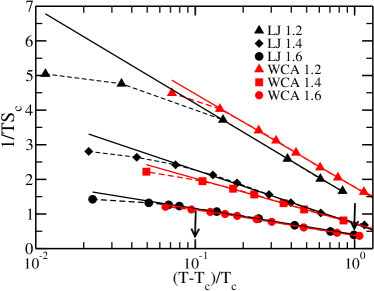
Figure 2: $\frac{1}{TS_{c}}$ plotted against $(\frac{T}{T_{c}}-1)$ and as predicted by Eq.15 the plot is linear in the region $10^{-1}\leq(\frac{T}{T_{c}}-1)\leq 10^{0}$ validating our claim that MCT power law region overlaps with AG region.

Although microscopic MCT shows a divergence of the relaxation time, $\tau$, at a much higher temperature Reichman than the glass transition temperature, the power law behaviour of $\tau$ as predicted by MCT is found to be valid in a range of low temperatures. Similar to the earlier studies szamel-pre ; tarjus_pre , the power law behaviour of simulated $\tau$ we compute is well described by an algebraic divergence given by,

$$\tau\sim(T-T_{c})^{-\gamma}\sim(\frac{T}{T_{c}}-1)^{-\gamma}$$ (14)

For all the densities we study, as shown in Fig.1, in a certain region of temperature, ($10^{-1}\leq(\frac{T}{T_{c}}-1)\leq 10^{0}$), the relaxation time ,$\tau$, for both LJ and WCA systems follow the MCT power law behaviour. On the other hand, the Adam Gibbs relation is also valid for all the systems in this region ($0\lesssim(\frac{T}{T_{c}}-1)\leq 10^{0}$) manu_under_prep . Thus we find that the temperature range where MCT like behaviour is predicted completely overlaps with the range where Adam-Gibbs relation is found to be valid. As mentioned in the Introduction this overlap regime has earlier been reported for other systems sciortino-pre-2002 . As in this temperature regime $\tau_{\alpha}$ can be described both by MCT power law behaviour and and by the AG relation we can write,

$$\frac{A}{TS_{c}}\propto-\gamma\ln(\frac{T}{T_{c}}-1)$$ (15)

In Fig.2 we show that $\frac{1}{TS_{c}}$ is linear when plotted against $\ln(\frac{T}{T_{c}}-1)$ in the region $10^{-1}\leq(\frac{T}{T_{c}}-1)\leq 10^{0}$ validating the statement that MCT like divergence region overlaps with AG region.

Figure 3: The temperature dependence of pair configurational entropy ($S_{c2}$) to determine Kauzmann temperature $T_{K2}$. $T_{K2}$ values are given in Table 1.

Since the configurational entropy has a finite value at the MCT transition temperature, $T_{c}$, the AG relation is not expected to predict a divergent relaxation time at this temperature. In order to investigate the origin of this avoided transition, we consider the separation of the configurational entropy into pair and many body parts as described earlier (sec-3.5)bssb . We find that the temperature dependence of ($S_{c2}$) is given by (Fig.3),

$$TS_{c2}=K_{T2}(\frac{T}{T_{K2}}-1)$$ (16)

where $K_{T2}$ is the pair thermodynamic fragility and $S_{c2}$ vanishes at the Kauzmann temperature $T_{K2}$ bssb . $T_{K2}$ is obtained from the linear fit of $TS_{c2}$ vs $T$ plot at $S_{c2}=0$. As reported earlier we find that for all the systems studied in this work the Kauzmann temperature for $S_{c2}$ is very close in value to the MCT transition temperature (Table 1).

Table 1: $T_{c}$ tarjus_berthier_jcp and $T_{K2}$ values are tabulated below. For all the systems studied here, the Kauzmann temperature for $S_{c2}$ is quite similar to the MCT transition temperature.

		$\rho=1.2$		$\rho=1.4$	$\rho=1.6$
	$T_{c}$	$T_{K2}$	$T_{c}$	$T_{K2}$	$T_{c}$	$T_{K2}$
LJ	0.435	0.445	0.93	0.929	1.76	1.757
WCA	0.28	0.268	0.81	0.788	1.69	1.696

Thus, although $S_{c}$ is finite at the estimated MCT $T_{c}$, $S_{c2}$ vanishes at $T_{K2}$ which coincides with $T_{c}$.

V Analytical Results

Our study shows that the AG theory which is based on activation dynamics can completely describe the mode coupling theory (MCT) power law behavior in the region where the latter is found to be valid (Fig.2). However, the microscopic picture for Mode Coupling Theory (MCT) and the Adam Gibbs (AG) relation are different. Either from the heuristic arguments of Adam and Gibbs, or from the Random First Order Transition (RFOT) derivation, the AG relation is obtained from an activation picture of the dynamics, whereas the MCT does not correspond to activated dynamics. This leads to the question of the role of entropy in MCT which will be the focus of this section.

V.1 Entropy and MCT

In the $k\rightarrow 0$ limit, the memory function, $\mathcal{M}(k,t)$ in Eq.10 can be rewritten as,

$$\mathcal{M}(k,t)=\frac{S(k)}{8\pi^{2}\rho k}\int_{0}^{\infty}dq\times q^{2}(S(q)-1)^{2}\times\phi^{2}(q,t)$$ (17)

In the Schematic MCT the $\phi(q,t)$ is usually decoupled from q, as in the memory function, $\mathcal{M}(k,t)$, the dominant contribution comes from the first peak of S(q) Bengtzelius ; leutheusser . Here we consider similar decoupling, however do not restrict ourself to first peak of S(q). Thus we write Eq.17 as

$$\mathcal{M}(k,t)=\frac{S(k)}{4\rho k(2\pi)^{3}}\left[\int_{0}^{\infty}d{\bf{q}}(S(q)-1)^{2}\right]\times\phi^{2}(k,t)$$ (18)

By writing S(q) in terms of g(r) we can rewrite Eq.18 as

$$\mathcal{M}(k,t)=\frac{S(k)}{2k}\times 2\pi\rho\left[\int drr^{2}(g(r)-1)^{2}\right]\phi^{2}(k,t)$$ (19)

Replacing $\mathcal{M}(k,t)$ from Eq.19 in Eq.9 and considering over damped limit by omiting the explicit ‘k’ dependence of $\phi(t)$, Eq.9 can be written in schematic form as

$$\dot{\phi}(t)+\Omega^{2}\phi(t)+\Omega^{2}\lambda\int_{0}^{t}dt^{\prime}\phi^{2}(t^{\prime})\dot{\phi}(t-t^{\prime})=0$$ (20)

Where we can identify the coupling parameter $\lambda$ from Eq.19 as

$$\lambda=\frac{S(k)}{2k}\times 2\pi\rho\int drr^{2}(g(r)-1)^{2}=-\frac{S(k)}{2k}\frac{S_{2approx}}{k_{B}}$$ (21)

Where we call $S_{2approx}$ as the approximate pair entropy. The choice of calling it entropy will become clear in the next analysis.

We note that the two body pair entropy is given by green_jcp ,

$$\frac{S_{2}}{k_{B}}=-2\pi\rho\int_{0}^{\infty}drr^{2}\{g(r)\ln g(r)-[g(r)-1]\}$$ (22)

Expanding the logarithmic term for $g(r)>0$ we get

$$\frac{S_{2}}{k_{B}}=-2\pi\rho\int_{0}^{\infty}drr^{2}[g(r)-1]^{2}\frac{1}{(g(r)+1)}+H$$ (23)

where in ‘H’ we put the higher order contributions. The Fig.4 shows that the primary contribution comes from the first term of Eq.23.

In the above equation we note that $r^{2}[g(r)-1]^{2}$ varies strongly compared to $1/(g(r)+1)$. In the later if we consider $g(r)\approx 1$ we can write

$$\frac{S_{2approx}}{k_{B}}=-2\pi\rho\int_{0}^{\infty}drr^{2}[g(r)-1]^{2}\sim 2\frac{S_{2}}{k_{B}}-2H$$ (24)

Our numerical analysis shows that for all the systems studied here $S_{2approx}$ vs $S_{2}$ is indeed linear (Fig.5) with a slope $\approx 2.5$.

Figure 4: The function ($\frac{S_{2}}{k_{B}}-H$) of Eq.23 and $S_{2}/k_{B}$ are plotted as a function of temperature. The plot shows that the primary contribution comes from the first term of the expansion.

Thus the coupling constant $\lambda$ is related to the pair entropy,

$$\lambda=-\frac{S(k)}{2k}\times\frac{S_{2approx}}{k_{B}}=-m_{s}\frac{S(k)}{2k}(S_{2}/k_{B}-H)$$ (25)

where $m_{s}$ is the slope obtained from $S_{2approx}$ vs $S_{2}$ plot.

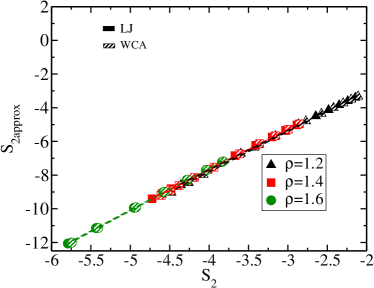
Figure 5: $S_{2approx}$ is plotted against $S_{2}$ and it shows a linear behaviour with a slope $\approx 2.5$.

The MCT relaxation time from schematic model leutheusser is given by

$$\tau\sim(1-\lambda)^{-\gamma}$$ (26)

Note that the power law behaviour of relaxation time $\tau$ (as given by Eq.26) changes to exponential dependence of $\tau$ under generalized MCT formalismjansen-reichman , when the coupling parameter is considered to be the same for all higher order terms and frequency $\Omega\sim 1$. With these conditions $\tau$ can be written as

$$\tau=\frac{1}{\Omega^{2}\lambda}(exp(\lambda)-1)\sim\frac{\exp(\lambda)}{\lambda}\sim C^{\prime}\exp(K^{\prime}S_{2})$$ (27)

The second equality is written by replacing $\lambda$ from Eq.25. Where $C^{\prime}$ and $K^{\prime}$ are not a constants, rather have a temperature dependence.

Earlier study of diffusion alok and our present microscopic derivation of the Rosenfeld relation for relaxation time $\tau$ shows that similar to Rosenfeld prediction, the MCT also predicts it to be an universal scaling law for all transport coefficients.

VI Numerical Results

VI.1 Rosenfeld scaling and MCT

In this section we analyze the MCT results in the light of Rosenfeld relation. We find that the relaxation time as obtained from microscopic MCT, $\tau_{MCT}$ when plotted against $\lambda$ does not follow the power law ($(1-\lambda)^{-\gamma}$) or $exp(\lambda)$ dependence in the whole temperature region. Usually it is found Ruchi_charu_2006 ; shankar_das that both $\tau_{MCT}$ and $\tau$ (relaxation time obtained from simulation) when plotted against $S_{2}$ does not show a single straight line. In Fig.6 we plot the $\tau_{MCT}$ calculated from Eq.9-12 against $S_{2}$ which shows two linear regimes. The origin of this break or the temperature dependence of the Rosenfeld parameter ‘$K^{\prime}$’ is not known.

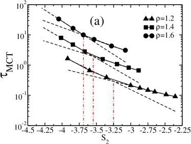
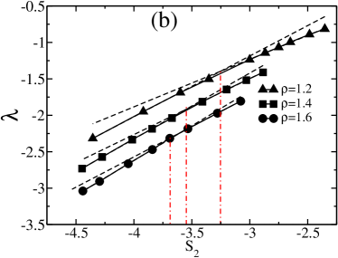
Figure 6: (a) The relaxation time obtained from microscopic MCT, $\tau_{MCT}$ is plotted against $S_{2}$. The dashed lines illustrate the two different Rosenfeld regimes. (b) Plot of $\lambda$ vs. $S_{2}$. This also shows two different linear regimes. For clarity $\tau$ and $\lambda$ are shifted by 1.2, 2.8 and -0.2, -0.48 for the systems of $\rho=1.4$ and $\rho=1.6$ respectively. The break in the slope for both the plots are illustrated by vertical dash-dot lines. We show that for a fixed density the break for both $\tau_{MCT}$ and $\lambda$ are at the same $S_{2}$ value.

Our analysis of Eq.25 shows that the Rosenfeld parameters are related to the static structure factor $S(k)$. Thus the temperature dependence of $S(k)$ leads to the temperature dependence of Rosenfeld parameter ‘$K^{\prime}$’. However since $S(k)$ changes continuously with temperature, it should lead to a similar temperature dependence of $K^{\prime}$. That a continuously changing ‘$K^{\prime}$’ is not needed to describe the observed behaviour but two distinct values suffice can be seen when we plot $\lambda$ against $S_{2}$ (Fig.6-b), where we see that there is a break in the slope and it happens at the same $S_{2}$ value where $\tau$ against $S_{2}$ shows a break in slope.

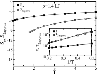
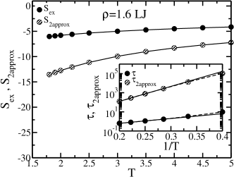
Figure 7: $S_{ex}$ and $S_{2approx}$ are plotted as a function of temperature for LJ and WCA systems at densities 1.2, 1.4 and 1.6. For all the systems $S_{2approx}$ has stronger temperature dependence and has smaller value than $S_{ex}$. In inset we plot $\tau_{2apporx}$ as obtained from Eq.30. It shows that $\tau_{2approx}$ has higher value and a larger slope leading to higher activation energy as compared to $\tau$. Activation energies are tabulated in Table 2

Next we show that the value of $S_{2approx}$ and its temperature dependence as compared to $S_{ex}$ can explain i) the larger values of $\tau_{MCT}$ as compared to $\tau$ szamel-pre ii) the higher values of activation energy as predicted by MCT tarjus_pre . When $E_{0}^{sim}$ and $E_{0}^{MCT}$ are obtained by fitting $\tau$ and $\tau_{MCT}$ to Arrhenius expression (Eq.28) we find values shown in Table 2, and in Fig.7.

$$\tau\sim\tau_{0}\exp\frac{E_{0}}{T}$$ (28)

Table 2: $E_{0}$ are tabulated for different systems. We show that the $E_{0}$ values are higher for MCT as well as for approximate calculation. As we can not calculate overlap function from MCT, for comparison of $E_{0}$ values we use simulated $F_{s}(k,t)$

		$\rho=1.2$		$\rho=1.4$	$\rho=1.6$
	LJ	WCA	LJ	WCA	LJ	WCA
$E_{0}^{sim}$	2.509	1.901	5.997	5.694	12.499	11.749
$E_{0}^{MCT}$	5.002	3.993	11.565	10.775	21.748	21.082
$E_{0}^{approx}$	6.224	5.705	16.535	15.831	37.159	36.564

Fig.7 shows that at all densities for both the systems $S_{2approx}$ is smaller than $S_{ex}$ and has a much stronger temperature dependence. Using Rosenfeld Expression we can write

$$\tau(T)=C\exp(-KS_{ex})$$ (29)

Now if we replace $S_{ex}$ by $S_{2approx}$, keeping C and $K$ same, we get

$$\tau_{2approx}=C\exp(-KS_{2approx})$$ (30)

The C and $K$ are obtained from linear fits of logarithmic of simulated relaxation time against excess entropy. Since $S_{2approx}<<S_{ex}$, the study shows that $\tau_{2approx}>>\tau$. Similar to that predicted by microscopic MCT (Eq.9, 11), the $E_{0}$ values for $\tau_{2approx}$ are higher, which are given in Table 2.

Although the results obtained from $\tau_{2approx}$ shows the correct trend, it can not match the parameters as obtained from $\tau_{MCT}$. We note that the $\tau_{2approx}$ is a prediction obtained from schematic MCT, which is known to overestimate the coupling constant $\lambda$. However this analysis not only explains the behaviour of MCT at high temperature, it also throws some light in the origin of its breakdown at low temperature. Usually the breakdown of MCT at low temperature has been attributed to the neglect of higher order correlation functions szamel-gmct ; jansen-reichman . This present analysis predicts that the stronger temperature dependence of the vertex might be partially responsible for the breakdown of MCT even at low temperature.

VI.2 The Adam Gibbs Relation and MCT

We have shown that the relaxation time ,$\tau$, over a temperature regime ($10^{-1}\leq(\frac{T}{T_{c}}-1)\leq 10^{0}$) follows both the AG relation and MCT power law behaviour. We also find the avoided divergence obeserved in the configurational entropy plot (Fig.2) arises from the vanishing of the pair configurational entropy ($S_{c2}$). For all the systems studied here, we find $T_{K2}\simeq T_{c}$ (Table 1), thus we can rewrite Eq.16 as,

$$TS_{c2}=K_{T2}(\frac{T}{T_{K2}}-1)\simeq K_{T2}(\frac{T}{T_{c}}-1)$$ (31)

We note that although $T_{K2}\simeq T_{c}$ and the MCT framework which predicts the power law behaviour is developed at the two body level, the AG relation with $S_{c2}$ alone cannot predict the MCT power law behaviour. and the RMPE ,$\Delta S$, plays an important role in predicting it. We also show that indeed there is a relation between MCT critical exponent $\gamma$, Adam Gibbs coefficient A, the pair thermodynamic fragility $K_{T2}$.

As shown earlier in Eq.13, configurational entropy can be written in terms of pair configurational entropy and RMPE. Thus we can write,

$$\frac{A}{TS_{c}}=\frac{A}{TS_{c2}+T\Delta S}=\frac{A}{K_{T2}}\frac{1}{[(\frac{T}{T_{c}}-1)+\frac{T\Delta S}{K_{T2}}]}$$ (32)

where we have used Eq.13 and Eq.31 to write the first and second equality respectively.

We find that although $T\Delta S$ is system dependent (Fig.8a), except for WCA system at $\rho=1.2$ the function $\frac{T\Delta S}{K_{T2}}$ shows a master plot when plotted against $(\frac{T}{T_{c}}-1)$ (Fig.8b). Note that although the value of $\frac{T\Delta S}{K_{T2}}$ is small, it is not negligible.

The master plot of $\frac{T\Delta S}{K_{T2}}$ can be fitted to a straight line, $\frac{T\Delta S}{K_{T2}}=0.26-0.35(\frac{T}{T_{c}}-1)$. Next we show that a function $\frac{1}{(\frac{T}{T_{c}}-1)+f(T)}$ when plotted against $\ln(\frac{T}{T_{c}}-1)$ shows linearity in the whole regime of $(10^{-1}\leq(\frac{T}{T_{c}}-1)\leq 10^{0})$ only when $f(T)$ is non-negligible positive quantity (Fig.8c). Note that in Fig.8c when $f(T)=0$ (which implies $\Delta S=0$ in Eq.32) the function diverges strongly. This shows that the AG relation at two body level cannot predict the MCT power law behaviour.

The analysis further shows that to obtain a correct estimation of the MCT power law exponent $\gamma$ (slope of the plot), $f(T)$ needs to obey the following temperature dependence, $f(T)=\frac{T\Delta S}{K_{T2}}=0.26-0.35(\frac{T}{T_{c}}-1)$. The two functions $\frac{T\Delta S}{K_{T2}}$ and $(\frac{T}{T_{c}}-1)$ show opposite trends, the former increases whereas the later decreases with temperature. Therefore a crossover between these two functions is observed in this regime and around MCT transition temperature, $\frac{T\Delta S}{K_{T2}}\gg(\frac{T}{T_{c}}-1)$ and configurational entropy and the relaxation time are determined primarily by many body contributions.

From Fig.8d we find in the temperature regime ($10^{-1}\leq(\frac{T}{T_{c}}-1)\leq 10^{0}$) Eq.32 can be re-written as,

$$\frac{A}{TS_{c}}=\frac{A}{K_{T2}}\frac{1}{[(\frac{T}{T_{c}}-1)+\frac{T\Delta S}{K_{T2}}]}\sim-\frac{mA}{K_{T2}}\ln(\frac{T}{T_{c}}-1)$$ (33)

where ‘m’ is the slope obtained from Fig.8(d) and given in Table 3. Since $\tau$ is found to follow AG relation we can write,

$$\tau\sim\exp(\frac{A}{TS_{c}})\sim(\frac{T}{T_{c}}-1)^{\frac{mA}{K_{T2}}}$$ (34)

Figure 8: (a) $T\Delta S$ is plotted as a function of $(\frac{T}{T_{c}}-1)$ and it shows a strong system dependence. (b) $\frac{T\Delta S}{K_{T2}}$ vs $(\frac{T}{T_{c}}-1)$ showing a master plot for all the systems except for WCA system at $\rho=1.2$. Dotted line is guide to eye. (c) $((\frac{T}{T_{c}}-1)+f(T))^{-1}$ plotted against $(\frac{T}{T_{c}}-1)$ by varying $f(T)$. Only for non negligible positive values of $f(T)$, linearity is found in the regime 0.1 to 1.0 of $(\frac{T}{T_{c}}-1)$. To obtain a correct estimation of the MCT power law exponent $\gamma$ (slope of the plot), f(T) needs to be temperature dependent (green dashed line). (d) $[\frac{1}{(\frac{T}{T_{c}}-1)+\frac{T\Delta S}{K_{T2}}}]$ vs $(\frac{T}{T_{c}}-1)$ shows a master plot for all the systems except for WCA system at $\rho=1.2$. ‘m’ is the slope of the linear plot which is tabulated in Table 3.

Table 3: The slope of the linear plot of $[\frac{1}{(\frac{T}{T_{c}}-1)+\frac{T\Delta S}{K_{T2}}}]$ vs $(\frac{T}{T_{c}}-1)$ in the region $(10^{-1}\leq(\frac{T}{T_{c}}-1)\leq 10^{0})$ (Fig.8d).

$\rho$	$m(LJ)$	$m(WCA)$
1.2	0.987	0.695
1.4	1.029	0.888
1.6	1.004	1.000

Table 4: $mA/K_{T2}$ and $\gamma$ for LJ and WCA system. As predicted by Eq.35 $mA/K_{T2}$ value is similar to $\gamma$ value obtained from free fitting (Fig.1 ) for most of the systems.

		$\rho=1.2$		$\rho=1.4$	$\rho=1.6$
	$mA/K_{T2}$	$\gamma$	$mA/K_{T2}$	$\gamma$	$mA/K_{T2}$	$\gamma$
LJ	2.322	2.229	2.474	2.385	2.352	2.299
WCA	2.932	2.243	2.852	2.289	2.579	2.304

Table 5: The Adam Gibbs coefficient ‘A’, as obtained from the linear fit of $\tau$ vs $1/TS_{c}$ plot, and pair thermodynamic fragility $K_{T2}$, as obtained from the linear fit of $TS_{c2}$ vs $T/T_{k2}$ plot for both the systems at different densities is tabulated below. The data shows that both are strongly dependent on density.

$\rho$	$A(LJ)$	$A(WCA)$	$K_{T2}(LJ)$	$K_{T2}(WCA)$
1.2	1.87	1.89	0.795	0.483
1.4	3.57	4.37	1.555	1.358
1.6	6.96	7.57	2.971	2.936

Comparing Eq.14 and Eq.34 we can write,

$$\frac{mA}{K_{T2}}\sim\gamma$$ (35)

where $m\simeq 1$ for all the systems except for the WCA system at $\rho=1.2$. Thus we show that the MCT scaling parameter, $\gamma$ is related to the AG parameter, A and the pair thermodynamic fragility of $S_{c2}$, $K_{T2}$. We have tabulated the $\gamma$ values in Table 4, which shows the above relation holds. The deviation of slope value (‘m’) from unity for WCA system at $\rho=1.2$ may have some connection to its breakdown of density-temperature scaling which needs to be investigated in future.

The MCT critical exponent ($\gamma$) is known to be density-temperature independent Gotze . Interestingly we also find that although both AG coefficient (A) and pair thermodynamic fragility ($K_{T2}$) are strongly dependent on density and temperature (Table 5), but their ratio, which is related to $\gamma$ (Eq.35), is density-temperature independent (Table 4).

VII Conclusion

In this work we show that in a certain region $(10^{-1}\leq(\frac{T}{T_{c}}-1)\leq 10^{0})$ the relaxation time follows both the AG relation and MCT power law behaviour. We also find that the MCT divergence temperatures coincide with the temperature where pair configurational entropy goes to zero for all the systems studied here. AG relation is based on activated dynamics, whereas MCT is mean field theory which at the two body level does not address any activated dynamics. Also the microscopic MCT does not have any apparent connection to entropy. Thus to understand the above mentioned observations we explore the connection between mode coupling theory and entropy and discuss different predictions of MCT in the light of entropy.

In this article we show that the MCT vertex for the structural relaxation time under certain approximations can be related to the pair excess entropy. Higher order MCT calculations in the schematic MCT framework can relate the relaxation time to the exponential of this vertex. Thus the MCT can provide a microscopic derivation of the phenomenological Rosenfeld theory. Our analysis shows that the Rosenfeld parameter is related to the static structure factor $S(k)$. The temperature dependence of $S(k)$ leads to the temperature dependence of Rosenfeld parameter ‘K’, thus explaining the earlier observation of the non-uniqueness of the Rosenfeld exponent shankar_das ; manish_charu . The analysis of the vertex reveals that quantity which contributes to the vertex, $S_{2apporx}$ has a much lower value and stronger temperature dependence as compared to the excess entropy , $S_{ex}$. If we assume the Rosenfeld scaling to be valid and replace $S_{ex}$ by $S_{2approx}$, the predicted relaxation time shows similar characteristics as the MCT relaxation time. Thus the study reveals that the larger value of $\tau_{MCT}$ and its higher activation energy is related to the value and temperature dependence of the vertex. This analysis further reveals that the breakdown of MCT at low temperature might be partially related to the strong temperature dependence of the vertex.

As mentioned earlier the AG theory which is based on activation dynamics can completely describe the mode coupling theory (MCT) power law behavior in the region where the latter is found to be valid. Since the configurational entropy has a finite value at the MCT transition temperature, $T_{c}$, the AG relation is not expected to predict any avoided transition in this regime. Our study reveals that although $S_{c}$ is finite, $S_{c2}$ vanishes at $T_{K2}$ (where $T_{K2}=T_{c}$), thus being responsible for the divergence like behavior. However we show that the pair configurational entropy although predicts the correct MCT transition temperature it by itself cannot predict the MCT power law behaviour. The residual multiparticle entropy (RMPE) plays an important role in providing the correct temperature dependence of relaxation time. We also obtain a connection between the AG coefficient (A), pair thermodynamic fragility ($K_{T2}$ and MCT critical exponent ($\gamma$) and found although first two quantities are dependent on density and temperature, their ratio which is related to $\gamma$, is density-temperature independent .

Note that although the absolute value of $\Delta S$ is in the similar range both at high and low temperature regimes, in the high temperature regime it plays a minor role in determining the dynamics, whereas its role at low temperature becomes central as we approach the avoided transition. This small positive value of $\Delta S$ playing an important role in predicting the MCT power law behaviour is similar to the prediction of unified theory sarika_PNAS . In the unified theory it was shown that in a certain temperature regime many body activated dynamics plays a hidden but central role in predicting the MCT like behaviour of the total relaxation time. Although apparently the MCT does not depend on the properties of landscape, the saddles in the landscape have been found to disappear at $T_{c}$ sciortino-saddles-prl ; sciortino-saddle ; wales_saddle ; sciortino-reply . Here we show that $S_{c2}$ also vanishes at $T_{c}$. Thus there may be a connection between pair configurational entropy and saddles. It will be also interesting to understand the independent role of pair configurational entropy and RMPE in the landscape picture. These are important open questions to be addressed in the future work.

VIII Acknowledgements

This work has been supported by the Department of Science and Technology (DST), India and CSIR-Multi-Scale Simulation and Modeling project. MKN thanks UGC and AB thanks DST for fellowship. Authors thank Prof. Kunimasa Miyazaki for discussions.

References

- (1) W. Götze and L. Sjögren, Zeitschrift für Physik B Condensed Matter 65, 415 (1987).
- (2) W. Götze, Journal of Physics: Condensed Matter 11, A1 (1999).
- (3) L. Berthier and G. Tarjus, Phys. Rev. Lett. 103, 170601 (2009).
- (4) L. Berthier and G. Tarjus, Phys. Rev. E 82, 031502 (2010).
- (5) L. Berthier and G. Tarjus, EPJE 34, 96 (2011).
- (6) L. Berthier and G. Tarjus, J. Chem. Phys. 134, 214503 (2011).
- (7) D. Coslovich, J. Chem. Phys. 138, 12A539 (2013).
- (8) D. Coslovich, Phys. Rev. E 83, 051505 (2011).
- (9) D. Kivelson, S. A. Kivelson, X. Zhao, Z. Nussinov, and G. Tarjus, Physica A: Statistical Mechanics and its Applications 219, 27 (1995).
- (10) S. Karmakar and I. Procaccia, Phys. Rev. E 86, 061502 (2012).
- (11) A. Malins and et al., J. Chem. Phys. 138, 12A535 (2013).
- (12) G. M. Hocky, T. E. Markland, and D. R. Reichman, Phys. Rev. Lett. 108, 225506 (2012).
- (13) A. Banerjee, S. Sengupta, S. Sastry, and S. M. Bhattacharyya, Phys. Rev. Lett. 113, 225701 (2014).
- (14) Y. Rosenfeld, Phys. Rev. E 62, 7524 (2000).
- (15) G. Adam and J. H. Gibbs, J. Chem. Phys. 43, 139 (1965).
- (16) Y. Rosenfeld, J Phys: Condens. Matter 11, 5415 (1999).
- (17) I. Borzsák and A. Baranyai, Chem. Phys. 165, 227 (1992).
- (18) M. Dzugutov, Nature 381, 6578 (1996).
- (19) J. J. Hoyt, M. Asta, and B. Sadigh, Phys. Rev. Lett. 85, 594 (2000).
- (20) J. Mittal, J. R. Errington, and T. M. Truskett, J. Chem. Phys. 125, 076102 (2006).
- (21) R. Sharma, S. N. Chakraborty, and C. Chakravarty, J. Chem. Phys. 125, 204501 (2006).
- (22) R. Zwanzig, PNAS 85, 2029 (1988).
- (23) S. Banerjee, R. Biswas, K. Seki, and B. Bagchi, J. Chem. Phys. 141, 124105 (2014).
- (24) A. Samanta, S. M. Ali, and S. K. Ghosh, Phys. Rev. Lett. 87, 245901 (2001).
- (25) C. Kaur, U. Harbola, and S. P. Das, J. Chem. Phys. 123, 034501 (2005).
- (26) M. Agarwal, M. Singh, B. Shadrack Jabes, and C. Chakravarty, J. Chem. Phys. 134, 014502 (2011).
- (27) Sengupta, Shiladitya, F. Vasconcelos, F. Affouard, and S. Sastry, J. Chem. Phys. 135, 194503 (2011).
- (28) S. Sengupta, S. Karmakar, C. Dasgupta, and S. Sastry, Phys. Rev. Lett. 109, 095705 (2012).
- (29) S. Mossa, E. La Nave, H. E. Stanley, C. Donati, F. Sciortino, and P. Tartaglia, Phys. Rev. E 65, 041205 (2002).
- (30) E. La Nave, A. Scala, F. W. Starr, F. Sciortino, and H. E. Stanley, Phys. Rev. Lett. 84, 4605 (2000).
- (31) E. La Nave, H. E. Stanley, and F. Sciortino, Phys. Rev. Lett. 88, 035501 (2002).
- (32) W. Kob and H. C. Andersen, Phys. Rev. E 51, 4626 (1995).
- (33) J. D. Weeks, D. Chandler, and H. C. Andersen, J. Chem. Phys. 54, 5237 (1971).
- (34) S. J. Plimpton, J. Comput. Phys. 117, 1 (1995).
- (35) M. Nauroth and W. Kob, Phys. Rev. E 55, 657 (1997).
- (36) S. Sastry, Phys. Rev. Lett. 85, 590 (2000).
- (37) S. Sastry, Nature 409, 164 (2001).
- (38) J. G. Kirkwood and E. M. Boggs, J. Chem. Phys. 10, 394 (1942).
- (39) R. E. Nettleton and M. S. Green, J. Chem. Phys. 29, 1365 (1958).
- (40) H. J. Raveché, J. Chem. Phys. 55, 2242 (1971).
- (41) D. C. Wallace, J. Chem. Phys. 87, 2282 (1987).
- (42) Y. Brumer and D. R. Reichman, Phys. Rev. E 69, 041202 (2004).
- (43) E. Flenner and G. Szamel, Phys. Rev. E 72, 031508 (2005).
- (44) manuscript under preparation.
- (45) W. G. U Bengtzelius and A. Sjolande, J. Phys. C: Solid State Phys 17, 5915 (1984).
- (46) E. Leutheusser, Phys. Rev. A 29, 2765 (1984).
- (47) L. M. C. Janssen, P. Mayer, and D. R. Reichman, Phys. Rev. E 90, 052306 (2014).
- (48) G. Szamel, Phys. Rev. Lett. 90, 228301 (2003).
- (49) S. M. Bhattacharyya, B. Bagchi, and P. G. Wolynes, PNAS 105, 16077 (2008).
- (50) L. Angelani, R. Di Leonardo, G. Ruocco, A. Scala, and F. Sciortino, Phys. Rev. Lett. 85, 5356 (2000).
- (51) L. Angelani, R. Di Leonardo, G. Ruocco, A. Scala, and F. Sciortino, J. Chem. Phys. 116, 10297 (2002).
- (52) J. P. K. Doye and D. J. Wales, J. Chem. Phys. 118, 5263 (2003).
- (53) L. Angelani, R. Di Leonardo, G. Ruocco, A. Scala, and F. Sciortino, J. Chem. Phys. 118, 5265 (2003).