Simulation of Time-dependent Heisenberg Models in 1D

Abstract

In this paper, we provide a theoretical analysis of strongly interacting quantum systems confined by a time-dependent external potential in one spatial dimension. We show that such systems can be used to simulate spin chains described by Heisenberg Hamiltonians in which the exchange coupling constants can be manipulated by time-dependent driving of the shape of the external confinement. As illustrative examples, we consider a harmonic trapping potential with a variable frequency and an infinite square well potential with a time-dependent barrier in the middle.

Introduction. – Strongly interacting quantum systems are an intricate and exciting part of theoretical physics. Their intricacy is due to the strong many-body correlations that may lead to unexpected new phenomena not present in the weakly-interacting case.

For systems with strong interparticle coupling, one spatial dimension (1D) plays a very special role Cazalilla et al. (2011). One reason for this is the unusual duality, often called the Fermi-Bose mapping, between 1D impenetrable bosons and ideal fermions, which was rigorously shown in 1960 by Girardeau Girardeau (1960). The most exciting aspect of this duality is the possibility to study it in modern experimental setups with two different atomic species Paredes et al. (2004); Kinoshita et al. (2004); Zürn et al. (2012). As a future perspective, the Fermi-Bose mapping suggests Volosniev et al. (2014); Deuretzbacher et al. (2014); Volosniev et al. (2015a); Levinsen et al. (2015) to engineer a chain of spins with adjustable nearest-neighbor couplings using a strongly repulsive multicomponent system in a trap Serwane et al. (2011); Pagano et al. (2014); Murmann et al. (2015). Such spin chains possess a very high degree of tunability thus opening the possibility of realizing and studying phenomena such as 1D $SU(N)$ quantum magnets and perfect state transfer Bose (2003); Volosniev et al. (2015a).

While the Fermi-Bose mapping was first established for a stationary system, the generalization to the case of a time-dependent trapping potential is straighforward for a system of impenetrable bosons Girardeau and Wright (2000a, b). To the best of our knowledge, however, such a generalization for multicomponent systems with large but finite interaction was not previously discussed in the literature . Due to the interplay of two different time-dependent effects, this generalization is far from obvious. First, there is the motion of particles due to the time-dependent trapping potential, and second, there is the particle exchange. As we will show the timescales for these effects are effectively decoupled from one another and the dynamics of particle exchange is determined by the trapping potential.

In this paper, we consider a system with two kinds of spinless fermions with strong interspecies repulsion. We first show that the behaviour of such a system can be described by the Heisenberg Hamiltonian with time-dependent exchange coupling coefficients. These coefficients can be altered by manipulating the shape of the trapping potential as a whole. This contrasts our idea with an idea of realizing a time-dependent Heisenberg Hamiltonian on a lattice by addressing every site independently. As we discuss below, our approach has very different strengths and limitations and thus ideally complements the standard lattice approach. In particular, it allows to address any trapping potential and is not limited to the lattice approximation. For a four-atom system this is sketched in Fig. 1. Part a) shows the initial configuration with two fermions in one well and two fermions of a different kind in the other well. We also sketch a possible evolution of this configuration in a time-dependent potential where the final state corresponds to the exchange of the two pairs. This evolution can be described by mapping the system to a spin-chain model described by a Heisenberg Hamiltonian where the coupling coefficients depend on time, see Fig. 1 b). The mapping opens a way to engineer and simulate driven Heisenberg Hamiltonians with time-dependent coefficients where the time dependence gives an extra knob to tune the dynamics in the system Lyakhov and Bruder (2006); Galve et al. (2009).

To illustrate our findings, we apply this mapping to a time-dependent harmonic potential and an infinite square well potential with a time-dependent barrier in the middle. For the former case, we show that the coupling coefficients in the spin chain are simply multiplied with a position independent scale factor. In the latter case, one can tune the middle coupling coefficient almost independently from the others. This allows one to achieve a controlled exchange of pairs, see Fig. 1 a).

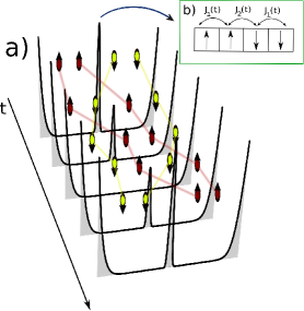
Figure 1: (Color Online). Mapping of a strongly interacting one-dimensional system in a time-dependent potential , a), onto a spin chain with time dependent coefficients, b).

Formulation. – For the sake of the argument let us start with a 1D system of $N$ spinless fermions of one kind (spin up) and one fermion of another kind (spin down). We assume that every particle has mass $m$ and is confined by the same time-dependent trapping potential $\varepsilon V(x/L,\varepsilon t/\hbar)$, where $\varepsilon=\hbar^{2}/(mL^{2})$ and $L$ is some natural time-independent unit of length. For convenience, we assume that $m=\hbar=L=1$ from now on.

The dynamics of a system with a spin-up fermion placed at $x$ and spin-down fermions at $y_{1},...,y_{N}$ is described by the wave function $\Psi(x,y_{1},...,y_{N},t)$, which satisfies the Schrödinger equation,

$$i\frac{\partial}{\partial t}\Psi=H\Psi,\qquad H=\sum_{i=1}^{N}h(y_{i},t)+h(x,t),$$ (1)

where $h(x,t)=-\frac{1}{2}\frac{\partial^{2}}{\partial x^{2}}+V(x,t)$ is the one-body Hamiltonian. The zero-range interaction enters through 1D Bethe-Peierls boundary conditions at the points where the particles meet (see e.g. Ref. McGuire (1965)):

$$\left(\frac{\partial\Psi}{\partial x}-\frac{\partial\Psi}{\partial y_{i}}\right)_{x=y_{i}^{+}}-\left(\frac{\partial\Psi}{\partial x}-\frac{\partial\Psi}{\partial y_{i}}\right)_{x=y_{i}^{-}}=2g\Psi(x=y_{i}),$$ (2)

where $g$ is the interaction strength and the notation $x=y_{i}^{\pm}$ means that the derivative is taken at the point $x=y_{i}\pm\varepsilon$, with $\varepsilon>0$ and the limit $\varepsilon\to 0$ is taken afterwards. Below, we consider the dynamics of the system in the following scenario: the interaction is adiabatically tuned in a constant trapping potential $V(x,0)$ from zero to some value $g^{f}$ which is very large. This procedure initializes the state $\Psi^{(0)}(x,y_{1},...,y_{N})$. It is assumed that at later times the shape of the trapping potential depends on time and we look for the wave function satisfying Eq. (1) with the initial condition $\Psi(t=0)=\Psi^{(0)}$.

Initial state. – Let us start by discussing the initial wave function $\Psi^{(0)}$. If $1/g^{f}=0$ then Eq. (2) dictates that the particles cannot exchange their relative positions and $\Psi^{(0)}$ should be described separately on each ordering of particles, e.g. $x<y_{1}<y_{2}<...<y_{N}$, on which the solution is obtained from the Fermi-Bose mapping Girardeau (1960):

$$\Psi^{(0)}=\sum_{j=1}^{N+1}a_{j}^{(0)}\chi_{j}(x,y_{1},...,y_{N})\Phi^{(0)}(x,y_{1},...,y_{N}),$$ (3)

where function $\chi_{j}$ is non-zero only if it contains $j-1$ arguments $y_{i}$ that are smaller than $x$, and $\Phi^{(0)}$ is one of the eigenstates of the Hamiltonian for $N+1$ spinless fermions (for the illustrative examples below we use the ground state). First note that the states from Eq. (3) are $N+1$-fold degenerate even if the eigenspectrum of spinless fermions is non-degenerate. Thus, to find $\Psi^{0}$, we should find the adiabatic eigenstates in $g$, that are characterized by $a_{j}^{(0)}$. This can be done perturbatively by minimizing the energy in the limit $g_{f}\to\infty$ Volosniev et al. (2014, 2015b); Gharashi et al. (2015). For large but finite interaction strengths, the wave function preserves the form given by Eq. (3) but acquires an additional contribution proportional to $1/g_{f}$. Furthermore, the minimization of energy leads to the mapping of a system onto a spin chain. To establish such a mapping in the time-dependent case, where the energy is not a good quantum number, a new approach is necessary and this is what we provide in this paper.

Time dynamics. – At $t>0$, the external potential depends on time and the time evolution is described by $\Psi(t)$. Let us first consider the system with infinite interaction, i.e. $1/g_{f}=0$. In this case, the wave function at each ordering should still be described with the wave function of spinless fermions Girardeau and Wright (2000a), $\Phi(x,y_{1},...,y_{N},t)$. Moreover, the probability of each ordering cannot be changed since the particles do not exchange their position. So $\Psi(t)$ in this limit has the same form as in Eq. (3) with $\Phi(t)$ instead of $\Phi^{(0)}$.

Let us now assume that the interaction strength is large but finite. Apparently this means that the wave function at each ordering cannot be described exactly with $\Phi^{(0)}$, and we should to look for a solution in the form $\Psi=\phi+\frac{1}{g_{f}}f$ where the function $\phi$ reads

$$\phi(x,y_{1},...,y_{N},t)=\sum_{j=1}^{N+1}a_{j}(t)\chi_{j}(x,y_{1},...,y_{N})\Phi.$$ (4)

Without any loss of generality, we assume that $\int f^{*}\chi_{i}\Phi\,\mathrm{d}x\,\mathrm{d}y_{1}...\mathrm{d}y_{N}=0$, i.e. that the functions $f$ and $\Phi$ are orthogonal on each ordering of the coordinates. Having in mind these conditions, we insert Eq. (4) in the Schrödinger equation. To proceed further, we insert the ansatz wave function into the Schrödinger equation and project it on each ordering. Next using that $f$ is orthogonal to $\Phi$ at every moment of time together with the boundary conditions (2), we eliminate the function $f$ (See Supplemental Material sup ). This procedure allows us to obtain a system of equations for the set of coefficients, $a_{j}(t)$,

$$i\frac{\mathrm{d}a_{j}}{\mathrm{d}t}=a_{j}(J_{j-1}+J_{j})-a_{j-1}J_{j-1}-a_{j+1}J_{j}+O\left(\frac{1}{g_{f}^{2}}\right),$$ (5)

where, assuming that $J_{0}=J_{N+1}=0$, the parameters $J_{i}$ are defined as follows

$$J_{j}(t)=-\frac{1}{g_{f}}\frac{\int_{y_{1}<y_{2}<...<y_{N}}\mathrm{d}y_{1}...\mathrm{d}y_{N}\left|\frac{\partial\Phi(t)}{\partial x}\right|^{2}_{x=y_{j}}}{\int_{x<y_{1}<y_{2}<...<y_{N}}\mathrm{d}x\mathrm{d}y_{1}...\mathrm{d}y_{N}\Phi^{2}(t)}.$$ (6)

After writing Eq. (5) in matrix form, it becomes apparent that up to the order $1/g^{2}_{f}$ this equation also describes the dynamics of a spin chain with the Heisenberg Hamiltonian

$$H_{s}=-\frac{1}{2}\sum_{j=1}^{N}J_{j}(t)(\bm{\sigma}^{j}\bm{\sigma}^{j+1}-\mathbf{I}),$$ (7)

and the corresponding wave function is

$$|F\rangle=\sum_{j=1}^{N+1}a_{j}(t)|\uparrow_{1}...\downarrow_{j}...\uparrow_{N+1}\rangle,$$ (8)

where we denote the identity operator on every site with $\mathbf{I}$, $\bm{\sigma}^{j}=(\sigma^{j}_{x},\sigma^{j}_{y},\sigma^{j}_{z})$ are the Pauli matrices acting on a spin at site $j$, and $J_{j}$ are site- and time- dependent interaction coefficients. Equations (7) and (8) generalize the time-independent mapping Volosniev et al. (2014); Deuretzbacher et al. (2014); Volosniev et al. (2015a) onto a spin-chain Hamiltonian to the time-dependent case. The derivation above implies that the time scale for the particle motion in leading order (in $1/g_{f}$) is determined by the trap alone, whereas the time scale of the spin exchange is proportional to $1/g_{f}$. It is related to the famous spin-charge separation Giamarchi (2004) in 1D, although here we derived it for a strongly interacting mesoscopic system from first principles in the presence of an external potential that depends on time. Note that there are higher order contributions to both, the particle motion and spin exchange. However, these corrections are negligible in the case of strong interactions, $1/g_{f}\to 0$, and therefore we do not need to consider them here.

Applying the presented approach it is easy to show that the Hamiltonian (7), can be used for any number of spin-down fermions similar to the time-independent case (see Ref. Volosniev et al. (2014) for a derivation). This is due to the fact that the main process in the system is the spin exchange of neighboring particles which is correctly described in the Hamiltonian (7). The same logic also applies to multicomponent system or systems made of strongly-interacting bosons.

Discussion. – We first assume that the coupling coefficients, $J_{i}$, are independent of time. Then linear system of equations (5) has the fundemental set of solutions: $a_{j}(t)=a^{(0)}_{j}e^{-i\epsilon t}$, where $\epsilon$ is the relevant eigenvalue of the Hamiltonian (7). Let us now consider what happens if the external trapping potential depends on time. To find the coefficients $J_{i}$ in this case, we first need to solve a time-dependent one-body problem and construct a Slater determinant wave function $\Phi$ out of the established solutions.

As our first application, we consider a system trapped by a harmonic oscillator potential, $V(x,t)=\omega^{2}(t)x^{2}/2$,  for which one-body solutions are known Husimi (1953); Popov and Perelomov (1969); Castin (2004); Moroz (2012), yielding $\Phi(x,y_{1},...,y_{N},t)$ from $\Phi^{(0)}$ as

$$\Phi=\frac{e^{-iE\int_{0}^{t}\frac{\mathrm{d}\tau}{\lambda^{2}(\tau)}}}{\sqrt{\lambda(t)^{N+1}}}e^{i\left(x^{2}+\sum_{i=1}^{N}y_{i}^{2}\right)\frac{\dot{\lambda}}{2\lambda}}\Phi^{(0)}\left(\frac{x}{\lambda},...,\frac{y_{N}}{\lambda}\right),$$ (9)

where $E$ is the initial energy and $\lambda(t)$ is the time-dependent scale parameter. Its time derivative $\dot{\lambda}$ is determined from the equation: $\lambda^{3}\ddot{\lambda}=1-\omega^{2}(t)\lambda^{4}(t)$. Since our choice of units sets $\omega^{2}(t<0)=1$, the initial conditions for this equation read $\lambda(t<0)=1$ and $\dot{\lambda}(t<0)=0$. Obviously, such a wave function $\Phi$ produces $J_{i}(t)\sim 1/\lambda^{3}(t)$, so that all coupling constants depend on time in the same way. The corresponding system of equations (5) has the following fundamental set of solutions: $a_{j}(t)=a_{j}^{(0)}e^{-i\epsilon\int_{0}^{t}\frac{\mathrm{d}\tau}{\lambda^{3}(\tau)}}$. Thus we see that the scale invariance given by the harmonic trap is preserved up to terms suppressed by $1/g_{f}$ in the form:

$$\Psi=\frac{e^{-i\epsilon\int_{0}^{t}\frac{\mathrm{d}\tau}{\lambda^{3}(\tau)}-iE\int_{0}^{t}\frac{\mathrm{d}\tau}{\lambda^{2}(\tau)}}}{\sqrt{\lambda(t)^{N+1}}e^{-i\left(x^{2}+\sum_{i=1}^{N}y_{i}^{2}\right)\frac{\dot{\lambda}}{2\lambda}}}\Psi^{(0)}\left(\frac{x}{\lambda},...,\frac{y_{N}}{\lambda}\right).$$ (10)

Therefore, the overall spin dynamics in the system is not affected by a change of the external potential up to corrections suppressed by $1/g_{f}$. Of course, the harmonic oscillator is a truly special case due to the scale invariance and any trapping potential that is not scale invariant will have more pronounced effects on the system. A detailed discussion of the breaking of scale invariance in the oscillator for two particles by higher order corrections can be found in Ref. Ebert et al. (2015).

It is interesting to note that the spin dynamics of the system in a harmonic trap can be altered by a time-independent weak magnetic field Volosniev et al. (2015a). With a magnetic field the Hamiltonian is $\tilde{H}=H+\sum_{i=1}^{N}\frac{b(y_{i})}{g_{f}}-\frac{b(x)}{g_{f}}$, where, for simplicity, we again consider a system with only one spin-down fermion . The correponding spin chain Hamiltonian is written as

$$\tilde{H}_{s}=-\frac{1}{2}\sum_{j=1}^{N}J_{j}(\bm{\sigma}^{j}\bm{\sigma}^{j+1}-\mathbf{I})+\sum_{j=1}^{N+1}\beta_{j}\sigma_{z}^{j},$$ (11)

where

$$\beta_{j}(t)=\frac{1}{g_{f}}\frac{\int\mathrm{d}y_{1}...\mathrm{d}y_{N}\mathrm{d}x\chi_{j}(x,y_{1},...,y_{N})|\Phi|^{2}\,b(x)}{\int\mathrm{d}y_{1}...\mathrm{d}y_{N}\mathrm{d}x\chi_{j}(x,y_{1},...,y_{N})|\Phi|^{2}}.$$ (12)

Notice that coefficients $\beta_{j}$ depend on time through $\Phi$ even though the magnetic field is stationary. However, since this time dependence can be different from $J_{i}(t)$ the probability of each ordering in the spin chain, i.e. $|a_{i}(t)|^{2}$ changes with time. An application of magnetic field can drive a transition to a spin segregated state where the spin down particles are not mixed with the spin up particles. As was discussed in Ref. Cui and Ho (2014), this is possible due to a high degeneracy of the spectrum such that even a tiny magnetic field gradient can drive such a transition. This can be utilized using the magnetic field in the form $b(x)=b_{0}x$, where $b_{0}$ is some constant parameter (therefore $\beta_{j}=\lambda(t)\beta_{j}^{(0)}$). By taking this constant to be large, such that $\beta_{j}(0)/J_{j}(0)\gg 1$, we can have the initial state to be almost fully spin segregated or ’ferromagnetic’. By increasing the frequency of the external confinement we can drive the system from dominantly ’ferromagnetic’ to ’antiferromagnetic’ states, since the Heisenberg Hamiltonian in Eq. (7) is ’antiferromagnetic’.

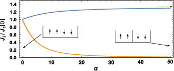
Figure 2: (Color Online). The coupling constants, $J_{i}/J_{1}(0)$ as functions of the barrier height, $\alpha$. The upper thick (blue) curve describes $J_{1}$, the lower (orange) curve corresponds to $J_{2}$. With the upper most arrow, we show the limiting value of $J_{1}$ for $\alpha\to\infty$. The insets show the system for the corresponding values of $\alpha$.

To conclude the presentation of the formalism, we consider a trapping potential where the quantum dynamics of a spin chain is altered without applying an external magnetic field. For this we use a potential schematically shown in Fig. 1, where a shallow area with a time-dependent barrier in the center is surrounded by impenetrable wells. We model this trap by an infinite square well potential, i.e. $V(x,t)=\alpha f(t)\delta(x)$ for $x\in[-1,1]$ and otherwise $V(x,t)\to\infty$. To give a spin chain time to react on the change of potential, we assume that $f(t)$ varies significantly only on a time scale given by $g_{f}$. This assumption means that $\Phi(t)$ changes almost adiabatically, which however does not imply adiabatic change of $\Psi(t)$ due to the degeneracy of the spectrum. Having this in mind, let us first assume that $f(t)=1$ and study $J_{i}$ for different $\alpha$. Note that conservation of parity leads to $J_{1}[\alpha]=J_{3}[\alpha]$. So it is enough to study only the combinations $J_{1}[\alpha]/J_{1}[0]$ and $J_{2}[\alpha]/J_{1}[0]$ which are $g_{f}$-independent and are shown in Fig. 2. For $\alpha=0$, we have a pure infinite square well potential which requires $J_{1}=J_{2}$. Positive values of $\alpha$ naturally descrease $J_{2}$ and increase $J_{1}$, such that for $\alpha\to\infty$, we have $J_{2}/J_{1}[0]\to 0$ and $J_{1}/J_{1}[0]\to 4/3$. The increase of $J_{1}[\alpha]/J_{1}[0]$ is related to the increase of the density in one well by increasing the barrier. Note that this effect should be less visible for more particles.

To illustrate the effect of this change of $J_{i}[\alpha]/J_{1}[0]$, we assume that for $\alpha\to\infty$ we prepare the system in the $\uparrow\uparrow\downarrow\downarrow$ configuration, see Fig. 1. Now we open and close the barrier and investigate the evolution of the system during this cycle. We assume the following form of the variation: $f(t)=(1-\sqrt{\sin(At/\tau)})$, where $\tau\equiv\pi/J_{1}[0]$ defines the natural time scale in the box in the absence of the barrier. Note that one cycle happens within the period $\pi/(A\tau)$. To supress the dynamics between different wells, we put $\alpha=50$ (see Fig. 2). We present our findings in Fig. 3, showing the probabilities of different configurations, i.e. $|a_{i}|^{2}$ for different $A$. Note that these probabilities after one cycle depend strongly on $A$ which provides a way for state preparation. For example let us take a look at the case with $A=0.8$ (panel c)). We see that for such a driving mode one ends up in $0.996\%$ of all cases in $\downarrow\downarrow\uparrow\uparrow$ which can be seen as the exchange of the pairs. Note, that if we had plotted the total density before and after the cycle for every configuration from Fig. 3, then we would have obtained the same result due to the adiabaticity of particle motion. Nevertheless, the spin configurations are profoundly different which highlights the separation of the spin and particle dynamics that we have derived. It is worthwhile noting that for even slower change of the potential with the time scale much larger than $g_{f}$ the dynamics in the both spin and charge sectors will be adiabatic.

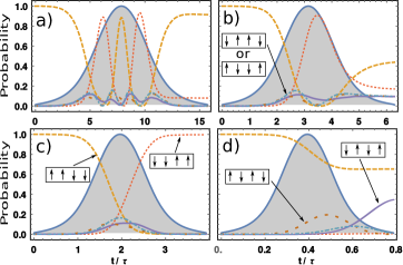
Figure 3: (Color Online.) Dynamics of probabilities for different configurations as a function of time for a four body system in an infinite square well potential with a time-independent barrier in the middle. Panel a) corresponds to $A=0.2$, b)  $A=0.5$, c)  $A=0.8$ and d)  $A=4$. The solid (blue) shaded curve shows the change of $J_{2}/J_{1}[0]$ as a function of time. Dashed (orange) curve depicts $\uparrow\uparrow\downarrow\downarrow$ configuration, dotted (red) - $\downarrow\downarrow\uparrow\uparrow$. These and all other configurations are shown in panels b), c) and d). Note that $\uparrow\downarrow\downarrow\uparrow$ and $\downarrow\uparrow\uparrow\downarrow$ configurations are equally probable.

Conclusions. – In this paper, we discuss a time dependent spin chain which is realized with strongly interacting atoms in a time-dependent confinement in 1D. First, we outline a mapping onto a spin chain for one impurity in a Fermi sea of majority particles. This mapping can be trivially extended to more impurity particles or other multicomponent strongly coupled systems. Next, we use a time-dependent harmonic oscillator potential with a weak stationary magnetic field and an infinite square well potential with a time-dependent barrier to illustrate some basic properties of the spin dynamics in such systems. In particular, we show that in the former case by changing the trapping potential one can drive a system to a spin segregated state. For the latter case, we demonstrate the possibility of a state preparation and manipulation by proper changing the shape of the trapping potential.

A major goal of cold atomic gas research is to reach the regime where quantum magnetism can be studied and a number of pioneering experiments have already been reported Anderlini et al. (2007); Fölling et al. (2007); Trotzky et al. (2008). In particular, the superexchange of two spins has been observed in Ref. Trotzky et al. (2008) and it was shown that the lattice spin model limit of the Bose-Hubbard model Kuklov and Svistunov (2003); Duan et al. (2003) could accurately describe the data. While limited to strong cooupling and 1D, the approach described here goes beyond those models as it can fully incorporate the shape of any (time-dependent) potential, circumventing any need for making a lattice approximation. Our approach therefore ideally complements the lattice approximation as a tool to simulate and study spin dynamics. This allows us to address the dynamical evolution of general $N$-body exchanges in arbitrary potentials in the strongly interacting limit for both fermionic and bosonic atoms. Our theory may therefore be relevant for using exchange interactions to generate multiparticle entanglement Briegel and Raussendorf (2001); Mandel et al. (2003) and building robust quantum gates Burkard et al. (1999); Petta et al. (2005) for use in quantum communication Korzh et al. (2015), computation, and information Nielsen and Chuang (2010).

Appendix A Supplemental Material for ”Simulation of Time-dependent Heisenberg Models in 1D”

Here we outline the derivation of Eq. (5) of the main text. For this we first insert the wave function $\Psi=\phi+\frac{1}{g_{f}}f$ in the Schrödinger equation. Next we make a projection onto a specific ordering by integrating the equation with $\chi_{j}\Phi^{*}$. This procedure yields

$$i\langle\chi_{j}\Phi|\Phi\rangle\frac{\mathrm{d}a_{j}(t)}{\mathrm{d}t}+ia_{j}\langle\chi_{j}\Phi|\frac{\partial\Phi}{\partial t}\rangle+\frac{i}{g_{f}}\langle\chi_{j}\Phi|\frac{\partial f}{\partial t}\rangle=\langle\chi_{j}\Phi|H|\phi\rangle+\frac{1}{g_{f}}\langle\chi_{j}\Phi|H|f\rangle\;.$$ (13)

To proceed, we notice that $H\chi_{j}\Phi=i\frac{\partial\chi_{j}\Phi}{\partial t}$ everywhere except at the points where the particles meet. We also notice that due to a non-smooth behaviour close to these points $H\chi_{j}\Phi$ yields a Dirac delta function. These observations allow us to conclude that

$$\langle\chi_{j}\Phi|H|\phi\rangle=ia_{j}(t)\langle\chi_{j}\Phi|\frac{\partial\Phi}{\partial t}\rangle.$$ (14)

Next we turn our attention to the $\langle\chi_{j}\Phi|H|f\rangle$ term in Eq. (13) which, for convenience, we rewrite as an integral over the configuration $y_{1}<y_{2}<...<y_{j-1}<x<y_{j}<...<y_{N}$,

$$\langle\chi_{j}\Phi|H|f\rangle=N!\int_{-\infty}^{\infty}\mathrm{d}y_{1}\int_{y_{1}}^{\infty}\mathrm{d}y_{2}...\int_{y_{i-1}}^{\infty}\mathrm{d}x\int_{x}^{\infty}\mathrm{d}y_{j}...\int_{y_{N-1}}^{\infty}\mathrm{d}y_{N}\mathrm{d}x...\mathrm{d}y_{N}\Phi^{*}Hf.$$ (15)

Our next steps are two integrations by parts. This will yield some boundary terms and the integral with $f$ and $\Phi$ exchanged. Notice that there will be two types of boundary terms: $i)$ with $y_{l}=y_{k}$, and $ii)$ with $x=y_{j-1}$ or $x=y_{j}$. The former terms vanish due to the fermionic nature of the majority particles. The latter, however, should be properly taken into account,

$$\frac{\langle\chi_{j}\Phi|H|f\rangle}{N!}=-\frac{1}{2}\lim_{\epsilon\to 0}\int_{y_{1}<y_{2}<...<y_{j-1}<x<y_{j}<...<y_{N}}\mathrm{d}x\mathrm{d}y_{1}...\mathrm{d}y_{N}\bigg{(}[\delta(x-y_{j}+\epsilon)-\delta(x-y_{j-1}-\epsilon)]\left(\Phi^{*}\frac{\partial f}{\partial x}-f\frac{\partial\Phi^{*}}{\partial x}\right)$$

$$+\delta(x-y_{j-1}-\epsilon)\left(\Phi^{*}\frac{\partial f}{\partial y_{j-1}}-f\frac{\partial\Phi^{*}}{\partial y_{j-1}}\right)-\delta(x-y_{j}+\epsilon)\left(\Phi^{*}\frac{\partial f}{\partial y_{j}}-f\frac{\partial\Phi^{*}}{\partial y_{j}}\right)-2fH\Phi^{*}\bigg{)},$$ (16)

where all but the last terms under the integral sign are the boundary terms. Thus, we have

$$\langle\chi_{j}\Phi|H|f\rangle=-i\langle f\chi_{j}|\frac{\partial\Phi}{\partial t}\rangle^{*}+\mathrm{boundary\;terms}\;.$$ (17)

Next, we collect the expressions just derived and write the equation for $a_{j}(t)$

$$i\frac{\mathrm{d}a_{j}(t)}{\mathrm{d}t}=\frac{1}{g_{f}}\frac{\mathrm{boundary\;terms}}{\langle\chi_{j}\Phi|\Phi\rangle},$$ (18)

where we used that $\frac{\mathrm{d}{\langle\chi_{j}\Phi|f\rangle}}{\mathrm{d}t}=0$ by construction. It is important to notice that Eq. (18) is general and does not rely on the assumption that $1/g_{f}$ is small. However, as we show below this assumption makes the derived expression very useful. Let us now focus on the boundary terms,

$$\mathrm{boundary\;terms}= -\frac{N!}{2}\lim_{\epsilon\to 0}\int_{y_{1}<y_{2}<...<y_{j-1}<x<y_{j}<...<y_{N}}\mathrm{d}x\mathrm{d}y_{1}...\mathrm{d}y_{N}f\times$$

$$\bigg{(}\delta(x-y_{j}+\epsilon)\left(\frac{\partial\Phi^{*}}{\partial y_{j}}-\frac{\partial\Phi^{*}}{\partial x}\right)+\delta(x-y_{j-1}-\epsilon)\left(\frac{\partial\Phi^{*}}{\partial x}-\frac{\partial\Phi^{*}}{\partial y_{j-1}}\right)\bigg{)}=$$

$$N!\int_{y_{1}<y_{2}<...<y_{j-1}<x<y_{j}<...<y_{N}}\mathrm{d}x\mathrm{d}y_{1}...\mathrm{d}y_{N}f\bigg{(}\delta(x-y_{j})-\delta(x-y_{j-1})\bigg{)}\frac{\partial\Phi^{*}}{\partial x}.$$ (19)

To obtain $f$ at the points where the particles meet, we use the boundary conditions from the main text. This yields

$$f(x=y_{i})=(a_{i+1}-a_{i})\frac{\partial\Phi}{\partial x}\bigg{|}_{x=y_{i}}+\frac{1}{2g_{f}}\left[\left(\frac{\partial f}{\partial x}-\frac{\partial f}{\partial y_{i}}\right)_{x=y_{i}^{+}}-\left(\frac{\partial f}{\partial x}-\frac{\partial f}{\partial y_{i}}\right)_{x=y_{i}^{-}}\right].$$ (20)

Now we make the assumption that $1/g_{f}\to 0$, which implies that $f(x=y_{i})\simeq(a_{i+1}-a_{i})\frac{\partial\Phi}{\partial x}\big{|}_{x=y_{i}}$. Inserting this result in Eqs. (19) and (18), we arrive at the desired expression. It should be noted that in our derivations we assume that $g_{f}$ sets the largest energy scale of the problem. Therefore, if the change of the trap is such that $g_{f}$ becomes of the order of the other energy scales then the treatment above is not valid, namely we cannot neglect the second term on the right-hand-side of Eq. (20). For example this can happen if we increase the density of the system, by squeezing the trap, which necessarily increases the kinetic energy. Another instance is a periodic driving in the parametric resonance region, which pumps in energy in the system.

References

- Cazalilla et al. (2011) M. A. Cazalilla, R. Citro, T. Giamarchi, E. Orignac, and M. Rigol, Rev. Mod. Phys. 83, 1405 (2011).
- Girardeau (1960) M. Girardeau, Journal of Mathematical Physics 1, 516 (1960).
- Paredes et al. (2004) B. Paredes, A. Widera, V. Murg, O. Mandel, S. Folling, I. Cirac, G. V. Shlyapnikov, T. W. Hansch, and I. Bloch, Nature 429, 277 (2004).
- Kinoshita et al. (2004) T. Kinoshita, T. Wenger, and D. S. Weiss, Science 305, 1125 (2004).
- Zürn et al. (2012) G. Zürn, F. Serwane, T. Lompe, A. N. Wenz, M. G. Ries, J. E. Bohn, and S. Jochim, Phys. Rev. Lett. 108, 075303 (2012).
- Volosniev et al. (2014) A. G. Volosniev, D. V. Fedorov, M. Jensen, A. S. Valiente, and N. T. Zinner, Nat. Commun. 5, 5300 (2014).
- Deuretzbacher et al. (2014) F. Deuretzbacher, D. Becker, J. Bjerlin, S. M. Reimann, and L. Santos, Phys. Rev. A 90, 013611 (2014).
- Volosniev et al. (2015a) A. G. Volosniev, D. Petrosyan, M. Valiente, D. V. Fedorov, A. S. Jensen, and N. T. Zinner, Phys. Rev. A 91, 023620 (2015a).
- Levinsen et al. (2015) J. Levinsen, P. Massignan, G. M. Bruun, and M. M. Parish, Science Advances 1, e1500197 (2015).
- Serwane et al. (2011) F. Serwane, G. Zürn, T. Lompe, T. B. Ottenstein, A. N. Wenz, and S. Jochim, Science 332, 336 (2011).
- Pagano et al. (2014) G. Pagano, M. Mancini, G. Cappellini, P. Lombardi, F. Schafer, H. Hu, X.-J. Liu, J. Catani, C. Sias, M. Inguscio, and L. Fallani, Nat. Phys. 10, 198 (2014).
- Murmann et al. (2015) S. Murmann, A. Bergschneider, V. M. Klinkhamer, G. Zürn, T. Lompe, and S. Jochim, Phys. Rev. Lett. 114, 080402 (2015).
- Bose (2003) S. Bose, Phys. Rev. Lett. 91, 207901 (2003).
- Girardeau and Wright (2000a) M. D. Girardeau and E. M. Wright, Phys. Rev. Lett. 84, 5691 (2000a).
- Girardeau and Wright (2000b) M. D. Girardeau and E. M. Wright, Phys. Rev. Lett. 84, 5239 (2000b).
- Note (1) Recent studies have considered time-dependent driving starting from the lattice approximation Itin and Katsnelson (2015). However we note that our formalism does not require one to make a lattice model approximation.
- Lyakhov and Bruder (2006) A. O. Lyakhov and C. Bruder, Phys. Rev. B 74, 235303 (2006).
- Galve et al. (2009) F. Galve, D. Zueco, S. Kohler, E. Lutz, and P. Hänggi, Phys. Rev. A 79, 032332 (2009).
- McGuire (1965) J. B. McGuire, Journal of Mathematical Physics 6, 432 (1965).
- Volosniev et al. (2015b) A. G. Volosniev, D. V. Fedorov, A. S. Jensen, and N. T. Zinner, Eur. Phys. J. Special Topics 224, 585 (2015b).
- Gharashi et al. (2015) S. E. Gharashi, X. Y. Yin, Y. Yan, and D. Blume, Phys. Rev. A 91, 013620 (2015).
- (22) See Supplemental Material .
- Giamarchi (2004) T. Giamarchi, Quantum Physics in One Dimension (Clarendon Press, Oxford, 2004).
- Husimi (1953) K. Husimi, Progress of Theoretical Physics 9, 381 (1953).
- Popov and Perelomov (1969) V. S. Popov and A. M. Perelomov, JETP 29, 738 (1969).
- Castin (2004) Y. Castin, Comptes Rendus Physique 5, 407 (2004).
- Moroz (2012) S. Moroz, Phys. Rev. A 86, 011601 (2012).
- Ebert et al. (2015) M. Ebert, A. Volosniev, and H. W. Hammer, (2015), arXiv:1512.06628 [cond-mat.quant-gas] .
- Note (2) Notice, that the resulting Hamiltonian can be straighforwardly generalized to more particles.
- Cui and Ho (2014) X. Cui and T.-L. Ho, Phys. Rev. A 89, 023611 (2014).
- Anderlini et al. (2007) M. Anderlini, P. J. Lee, B. L. Brown, J. Sebby-Strabley, W. D. Phillips, and J. V. Porto, Nature (London) 448, 452 (2007).
- Fölling et al. (2007) S. Fölling, S. Trotzky, P. Cheinet, M. Feld, R. Saers, A. Widera, T. Müller, and I. Bloch, Nature (London) 448, 1029 (2007).
- Trotzky et al. (2008) S. Trotzky, P. Cheinet, S. Fölling, M. Feld, U. Schnorrberger, A. M. Rey, A. Polkovnikov, E. A. Demler, M. D. Lukin, and I. Bloch, Science 319, 295 (2008).
- Kuklov and Svistunov (2003) A. B. Kuklov and B. V. Svistunov, Phys. Rev. Lett. 90, 100401 (2003).
- Duan et al. (2003) L.-M. Duan, E. Demler, and M. D. Lukin, Phys. Rev. Lett. 91, 090402 (2003).
- Briegel and Raussendorf (2001) H. J. Briegel and R. Raussendorf, Phys. Rev. Lett. 86, 910 (2001).
- Mandel et al. (2003) O. Mandel, M. Greiner, A. Widera, T. Rom, T. W. Hänsch, and I. Bloch, Nature (London) 425, 937 (2003).
- Burkard et al. (1999) G. Burkard, D. Loss, and D. P. Divincenzo, Phys. Rev. B 59, 2070 (1999).
- Petta et al. (2005) J. R. Petta, A. C. Johnson, J. M. Taylor, E. A. Laird, A. Yacoby, M. D. Lukin, C. M. Marcus, M. P. Hanson, and A. C. Gossard, Science 309, 2180 (2005).
- Korzh et al. (2015) B. Korzh, C. C. W. Lim, R. Houlmann, N. Gisin, M. J. Li, D. Nolan, B. Sanguinetti, R. Thew, and H. Zbinden, Nature Photonics 9, 163 (2015).
- Nielsen and Chuang (2010) M. A. Nielsen and I. L. Chuang, Quantum Computation and Quantum Information, by Michael A. Nielsen, Isaac L. Chuang (Cambridge, UK: Cambridge University Press, 2010).
- Itin and Katsnelson (2015) A. P. Itin and M. I. Katsnelson, Phys. Rev. Lett. 115, 075301 (2015).