Controlling photon transport in the single-photon weak-coupling regime of cavity optomechanics

Abstract

We study the photon statistics properties of few-photon transport in an optomechanical system where an optomechanical cavity couples to two empty cavities. By analytically deriving the one- and two-photon currents in terms of a zero-time-delayed two-order correlation function, we show that a photon blockade can be achieved in both the single-photon strong-coupling regime and the single-photon weak-coupling regime due to the nonlinear interacting and multipath interference. Furthermore, our systems can be applied as a quantum optical diode, a single-photon source, and a quantum optical capacitor. It is shown that this the photon transport controlling devices based on photon antibunching does not require the stringent single-photon strong-coupling condition. Our results provide a promising platform for the coherent manipulation of optomechanics, which has potential applications for quantum information processing and quantum circuit realization.

I introduction

The nonlinear effect is potential resource for quantum information processing QIP . For example, the photon blockade resulting from the nonlinearity is employed in single-photon (few-photon) transmission control TC and optical state truncation ST . Similarly, photon blockade is also an important feature in a lot of quantum device design such as fast two-qubit controlled-NOT gate CNOT , efficient quantum repeaters EQR , single-photon transistor SPT and optical quantum computer QC . The rectifying device related with nonlinearity is the key device to information processing in integrated circuits ED . Considerable efforts has been made to investigate the optical diodes OD . Recently, various possible solid-state optical diodes have been proposed, for example the diodes from standard bulk Faraday rotators FR , integrated on a chip CP , realized in opto-acoustic fiber OF and from moving photonic crystal MPC . A kind of optical diode based on photon blockade effect also have been proposed, including photonic diode by a nonlinear-linear junction of coupled resonators OPD and optical diode of two semiconductor microcavities coupled via $\chi^{(2)}$ nonlinearities MOD .

The nonlinear interaction between optical and mechanical modes arising from radiation pressure force in optomechanical (OM) systems exhibit a lot of interesting nonlinear effects such as photon (phonon) blockade PB1 ; PB2 , optomechanical induced transparency OMIT1 ; OMIT2 and Kerr nonlinearity Kerr1 ; Kerr2 . Cavity optomechanics has received significant attention both in fundamental experiments FE1 ; FE2 and sensing applications SD1 ; SD2 . Currently, experimental technique of cavity optomechanics are still in the single-photon weak coupling regime RVOM ($g^{2}<\kappa\omega_{m}$), meanwhile it draws relatively few of works as control devices in quantum information processing because the prerequisite of the strong nonlinear is required OMD1 ; OMD2 . In order to utilize the nonlinearity of OM system in quantum information control, much attention has been paid to the photon blockade in OM system, including quadratically coupled OM systems QOM , hybrid electro-optomechanical system HOM , and ultrastrong optomechanics UOM , where the strong coupling condition is required. Ref. ABPB2 has shown that strong photon antibunching can be achieved in two coupled cavities with weak Kerr nonlinearity, which motivate us try to achieve strong nonlinear effect in OM system in weak coupling regime. In this paper, we propose a scheme to realize an optical diode with optomechanical cavity coupled to two cavities. This scheme does not require the stringent condition that the single-photon optomechanical coupling strength $g$ is on the order of the mechanical resonance frequency $\omega_{m}$ PB2 or the coupling strength $g$ is larger than the cavity decay rate $\kappa$ QOM . Our results show that photon blockade can be achieved both in strong and weak coupling regime because of the nonlinearity and the multipath interference. By examining the second-order correlation function, rectifying factor $\mathcal{R}$ and transport efficiency $\mathcal{T}$, we exhibit the characteristics of our system as photonic diode. Meanwhile, the single-photon transport can be controlled by the tuning of the frequency of the cavities in strong coupling regime. Surprisingly, by pumping two sides of the system (cavity $L$ and $R$), the device will embodies some characteristics like capacitor: photon storage-release (charge-discharge) and filtering of photon frequency.

The paper is organized as follows. In Sec. II, we introduce the system and eigensystem of Hamiltonian. We discuss photons transport control in the cavity optomechanical system as diode and capacitor in Sec. III. Discussion and conclusions are given in Sec. IV.

II Model and Hamiltonian

We consider a compound optomechanical system in which a cavity with a movable mirror is coupled with two cavities (L and R) with the coupling constant $J_{L}$ and $J_{R}$, see Fig. 1. The system described by the Hamiltonian $H=H_{sys}+H_{pump}$. By setting $\hbar=1$, the Hamiltonian $H_{sys}$ reads

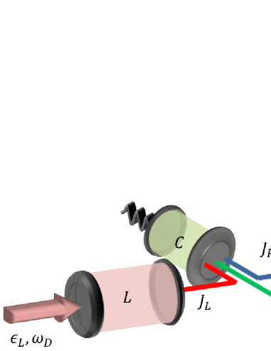
Figure 1: (Color online). Schematic of the cavity optomechanical system coupled with two cavities. Cavities $L$, $R$ and $C$ all can driven by the laser field with same frequency.

$$H_{sys} = \sum_{j=L,C,R}\omega_{l}a_{j}^{\dagger}a_{j}+\omega_{m}b^{\dagger}b+g(b^{\dagger}+b)a_{C}^{\dagger}a_{C}$$ (1)

$$+(J_{L}a_{L}^{\dagger}a_{C}+J_{R}a_{R}^{\dagger}a_{C}+h.c.),$$

where $a_{C}$, $a_{L}$ and $a_{R}$ are the annihilation operator for the photon mode of cavities $C$, $L$ and $R$ with frequency $\omega_{C}$, $\omega_{L}$ and $\omega_{R}$, respectively. $b$ is the phonon annihilation operator of the mechanical mode for the mirror with frequency $\omega_{m}$, $g$ denote the coupling strength of radiation pressure. The cavity modes are driven by the laser with the same frequency $\omega_{D}$, which can be described by $H_{pump}=\sum_{j=L,C,R}\varepsilon_{j}(a_{j}^{\dagger}e^{-i\omega_{D}t}+h.c.)$. In the rotating frame with $H_{0}=\sum_{j=L,C,R}\omega_{D}a_{j}^{\dagger}a_{j}$, we obtain

$$H_{S} = \sum_{j=L,C,R}\Delta_{j}a_{j}^{\dagger}a_{j}+\omega_{m}b^{\dagger}b+g(b^{\dagger}+b)a_{C}^{\dagger}a_{C}$$ (2)

$$+(J_{L}a_{L}^{\dagger}a_{C}+J_{R}a_{R}^{\dagger}a_{C}+h.c.)$$

$$+\sum_{j=L,C,R}\varepsilon_{j}(a_{j}^{\dagger}+a_{j}),$$

where $\Delta_{j}=\omega_{j}-\omega_{D}$ $(j=L,C,R)$ are the detuning between the driving field and the $jth$ cavity frequency, respectively. For this cascade configuration, cavity L and R are used as input and output ports in the side L and R. In this case, optomechanical cavity as an assisted-cavity, provides an intrinsically nonlinear interaction.

We assume that the cavities ($L$ and $R$) incoherently dissipate at rates $\kappa_{l}$ $(l=L,R)$ determined by the openness of the output channels and only classical driving fields are added to the quantum vacuum of the system, then according to the standard input-output relation ITR , the average output current (or photon stream) as number of quanta emitted at time $t$ from each cavity can be formally given by

$$Q_{l}(t)=\kappa_{l}\emph{Tr}[a_{l}^{{\dagger}}a_{l}\rho(t)],(l=L.R),$$ (3)

where $\rho$ is the density operator of system. The evolution of the density operator $\rho$ for the Hamiltonian $H_{S}$ can be described by the master equation

$$\dot{\rho} = -i[H_{S},\rho]+\sum_{j=L,C,R}\frac{\kappa_{j}}{2}\mathcal{D}[a_{j}]\rho+\frac{\gamma}{2}(n_{th}+1)\mathcal{D}[b]\rho$$ (4)

$$+\frac{\gamma}{2}n_{th}\mathcal{D}[b^{\dagger}]\rho,$$

where $\kappa_{j}$ and $\gamma$ are the cavity and mechanical energy decay rates, $n_{th}=[exp(\omega_{m}/k_{B}T_{M}-1)]^{-1}$ is the average thermal occupancy number of the oscillator. $\mathcal{D}[o]=2o\rho o^{\dagger}-o^{\dagger}o\rho-\rho o^{\dagger}o$ is the Lindblad dissipation superoperator.

The eigen equation of the Hamiltonian $H_{om}=\omega_{m}b^{\dagger}b+\Delta_{C}a^{\dagger}a+g(b^{\dagger}+b)a^{\dagger}a$ can be expressed as

$$H_{om}|s\rangle_{C}|\tilde{n}(s)\rangle_{m}=E_{s,n}|s\rangle_{C}|\tilde{n}(s)\rangle_{m},$$

where the eigenvalues are

$$E_{s,n}=s\Delta_{C}+n\omega_{m}-s^{2}\delta,$$

with $\delta=\frac{g^{2}}{\omega_{m}}$, and the eigenstate

$$|\tilde{n}(s)\rangle=e^{g(b-b^{\dagger})/\omega_{m}}|n\rangle$$ (5)

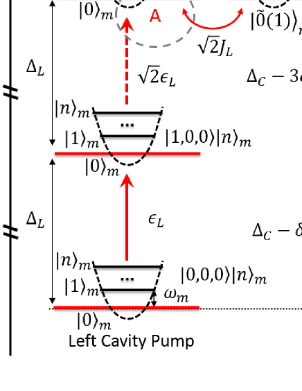
Figure 2: (Color Online) The eigensystem of the Hamiltonian $H_{S}$ in the zero-, one-, and two-photon cases, sub-area $A$, $B$ and $C$ denote multi-path interference in the system

is the displaced number state. The eigensystem of the Hamiltonian $H_{S}$ in the zero-, one-, and two-photon cases is shown in Fig. 2. We noticed that, the energy levels for optomechanical cavity (middle green line) will obtain a shift $s^{2}\delta$ caused by the nonlinear interacting with a frequency red (blue) detuning from the resonator resonance. This nonlinear shift can lead to bunched or antibunched photons in the OM cavity (the details are given in Sec. III C). This nonlinear effects also can appear in other cavities because of the coupling $J_{L}$ and $J_{R}$. Especially in strong coupling regime $g/\kappa\gg 1$, the system appears photon blockade, i.e. the probability for two photons inside the cavity is largely suppressed due to the energy restriction.

The interference between multipath for two-photon excitation in cavities are partially responsible for the photon antibunching effect shown in the sub-area of eigensystem diagram A, B and C. For area A, the two-photon in cavity $L$ with state $|2,0,0\rangle|n\rangle_{m}$ have two excitation path, one is direct excitation from low level in cavity $L$ with state $|1,0,0\rangle|n\rangle_{m}$, the other is the tunnelling from OM cavity to left cavity with state $|1,1,0\rangle|\tilde{n}\rangle_{m}$. The destructive interference between the two paths reduces the probability of two-photon excitation in the cavity. As well as area B and C. When the probability equal to zero, unconventional photon blockade ABPB1 ; ABPB2 ; UPB appears in the cavity with no requirement to strong nonlinear coupling coefficient $g$ (even $g/\kappa<1$). Therefore, the compound optomechanical system can work as a single photon control device both in OM weak- and strong- coupling regime, which will be discussed in detail in next section.

III Photons transport control in the cavity optomechanical system

III.1 Optomechanical optical diode

When the nonlinear effect for the right-going ($k$) is different from that for the left-going ($-k$) waves, i.e. the nonlinearity of the composite system is asymmetric, the rectification of one-dimensional photons transport can be controlled. The one way transport is called optical diode OD . In this section, we will show that our compound system can worked as a photonic diode.

We are interested in the statistic property of photons and its control. Usually, the frequency of the mechanical oscillator is larger than the strength of coupling of the radiation pressure, i.e., $\omega_{m}\gg g$. For simplicity, we can adiabatically eliminating the degree of the oscillators. Including the decay rate of the cavities, we have non-Hermitian effective Hamiltonian as

$$H_{eff} = \sum_{j=L,C,R}[(\Delta_{j}-i\kappa_{j}/2)a_{j}^{{\dagger}}a_{j}+\varepsilon_{j}(a_{j}^{{\dagger}}+a_{j})]$$ (6)

$$-i\sum_{j=L,C,R}\frac{\kappa_{j}}{2}a_{j}^{\dagger}a_{j}-\delta a_{C}^{{\dagger}}a_{C}-\delta a_{C}^{{\dagger}}a_{C}^{{\dagger}}a_{C}a_{C}$$

$$+(J_{L}a_{L}^{{\dagger}}a_{C}+J_{R}a_{R}^{{\dagger}}a_{C}+h.c.).$$

We assume that the general state is

$$|\psi(t)\rangle = C_{0}(t)|{\o}\rangle+\sum_{j=L,C,R}C_{j}(t)a_{j}^{{\dagger}}|{\o}\rangle$$ (7)

$$+\sum_{i,j=L,C,R}\frac{1}{2}C_{ij}(t)a_{i}^{{\dagger}}a_{j}^{{\dagger}}|{\o}\rangle.$$

Under weak pumping conditions, we have ABPB2

$$C_{0}\gg C_{j}\gg C_{ij}.$$

Under this condition, one can obtain the steady state solution of the probability amplitudes, see Appendix.

And the effect of quantum nonlinear features can be characterized by the second-order correlation function with zero-time delay.

$$g_{j}^{(2)}(0)=\frac{\langle a_{j}^{{\dagger}2}a_{j}^{2}\rangle}{\langle a_{j}^{{\dagger}}a_{j}\rangle^{2}},j=L,R,C.$$ (8)

We notice that $g_{j}^{(2)}(0)<1$ indicates photon antibunching and $g_{j}^{(2)}(0)>1$ indicates photon bunching, respectively. Antibunching corresponds to a reduced probability of two photons in the cavity at a given time, which is the opposite for bunching. The probability of two photons in the cavity will equal to zero if $g_{j}^{(2)}(0)\approx 0$ (photon blockade). For simplify, we set $\kappa_{L}=\kappa_{R}=\kappa_{C}=\kappa$, $\alpha_{j}=\Delta_{j}-i\kappa/2$ $(j=L,C,R)$. If $\alpha_{L}=\alpha_{R}=\alpha,\varepsilon_{L}=\varepsilon$ and $\varepsilon_{C},\varepsilon_{R}=0$, i.e., the system is only pumped on the left cavity with the magnitude $\varepsilon$, the photon second-order correlation function with no time-delay in left cavity can be obtained

$$g_{L}^{(2)}(0) = |\frac{J_{R}^{4}K_{2}+(J_{L}^{2}-J_{R}^{2})K_{1}F_{2}}{(J_{L}^{2}+J_{R}^{2})K_{2}-K_{1}F_{2}}-F_{1}|^{2}$$ (9)

$$\times|\frac{\left(J_{L}^{2}+J_{R}^{2}-F_{1}\right)}{\left(J_{R}^{2}-F_{1}\right){}^{2}}|^{2},$$

where $K_{n}=\alpha+\alpha_{C}+n\delta$ and $F_{n}=\alpha(\alpha_{C}+n\delta)$ ($n=1,2$). Setting $\Delta_{L}=\Delta_{R}=\Delta_{C}=\Delta$, we plot logarithmic $g_{L}^{(2)}(0)$ as a function of $\Delta$ and $g$ in Fig. 3a. $g_{L}^{(2)}(0)\approx 0$ represents photon blockade, corresponding to the dark areas, which appears in two areas. The one is achieved in the low-right area in Fig. 3a with large values of coupling rate $g$, which means that the photon blockade is resulted from the nonlinear effects of radiation pressure. We call it conventional photon blockade (CPB). And the other appears in up-left with small values of $g$ but strict limitations on other parameters, which means that it is resulted from the two-path interference. The interference between the two excitation path (the one exciton is from its own exciton, and the other is the jumping from its neighbor) is illustrated in Fig. 3b. Because of the destructive interference, the photon blockade phenomenon is also appearance, called unconventional photon blockade (UPB).

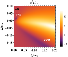
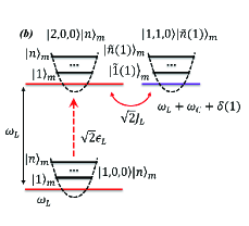
Figure 3: (Color online) (a)The zero-time second-order correlation $g_{L}^{(2)}(0)$ as a function of the coupling strength $g$ and the driving detuning $\Delta$ (log scale). Other parameters are $J_{L}/\omega_{m}=0.5$, $J_{R}/\omega_{m}=0.01$, $\kappa/\omega_{m}=0.036$. (b) The eigensystem of two excitation path interference in cavity $L$.

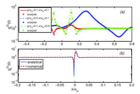
Figure 4: (Color online) The equal-time second-order correlation $g_{L}^{(2)}(0)$ as a function of the coupling strength $g$ and the driving detuning $\Delta$, set $\Delta_{L}=\Delta_{C}=\Delta$, $\Delta_{R}=\Delta+\Delta_{LR}$. Other parameters are (a) $J_{L}/\omega_{m}=0.5$, $J_{R}/\omega_{m}=0.1$, $\Delta_{LR}=0$. (b) $J_{L}/\omega_{m}=0.1$, $J_{R}/\omega_{m}=0.01$, $g/\omega_{m}=0.01$, $\kappa/g=1.3$, $\Delta_{LR}=0.1$ (other groups of parameters can be get by solving $g_{L}^{(2)}(0)=0$ in weak coupling regime).

We now show the photon statistics properties and the controlling of the photon transport by comparing the analytical solution with the numerical results via solving the master equation (4). For the conventional photon blockade, the larger the ratio of $g/\kappa$, the stronger the effect of blockade, shown in Fig. 4a. The corresponding detuning frequency can be derived from Eq. (9). As shown in Fig. 4b, the strong photon antibunching can be obtained even if $g/\kappa<1$.

In order to describe the characteristics of unidirectional energy transport. We define the rectifying factor $\mathcal{R}$ and transport efficiency $\mathcal{T}$ as the normalized difference between the output currents when the system is pumped through the left and right resonator (indicated by the wave vectors $k$ and $-k$, respectively) OPD

$$\mathcal{R} = \frac{Q_{R}[k]-Q_{L}[-k]}{Q_{R}[k]+Q_{L}[-k]},$$ (10)

$$\mathcal{T}_{L} = \frac{Q_{R}[k]}{Q_{R}[k]+Q_{L}[k]},$$ (11)

$$\mathcal{T}_{R} = \frac{Q_{L}[-k]}{Q_{R}[-k]+Q_{L}[-k]}.$$ (12)

$\mathcal{R}=-1$ indicates maximal rectification with enhanced transport to the left (left rectification), $\mathcal{R}=0$ indicates no rectification because $Q_{R}[+k]=Q_{L}[-k]$, while $\mathcal{R}=+1$ indicates maximal rectification with transport to the right (right rectification). In our system, cavity $L$ and cavity $R$ are both linear cavity. Therefore, there is no rectification ($\mathcal{R}=0$) when only driving the left or right cavity (no asymmetric nonlinear effect).

We discuss the rectification effect in conventional blockade regime ($\omega_{m}>g>\kappa$) shown in Fig. 5. When $\frac{\Delta}{\omega_{m}}$ is around $-0.02$, $\mathcal{R\approx}+1$ which indicates that the system allows photon transfer from left to right $L\rightarrow R$ only, and the transfer is prohibited from right to left $R\rightarrow L$, the photon number from left-going ($-k$) field equal to zero in side $L$. Similarly, when $\frac{\Delta}{\omega_{m}}$ is around 0.005, $\mathcal{R}=-1$, which only allows the transport from right to left $R\rightarrow L$ and $N_{R}(k)=0$. For $\frac{\Delta}{\omega_{m}}$ is around -0.005, $\mathcal{R}=0$, the photon number from left-going ($-k$) field equal to the photon number from right-going ($k$) field $N_{L}(-k)=N_{R}(k)$. If $g<\kappa<\omega_{m}$ (unconventional blockade regime), shown in Fig. 6, one can obtain $\mathcal{R}\approx+1$ when $\frac{\Delta}{\omega_{m}}=0.022$. We also can see $\mathcal{R}=0$ for $\frac{\Delta}{\omega_{m}}=0.015$, and $\mathcal{R}\approx-1$ for $\frac{\Delta}{\omega_{m}}=0.003$. Therefore we can conclude that no matter $\omega_{m}>g>\kappa$ or $g<\kappa<\omega_{m}$ by tuning the frequencies of the cavity $R$ and $L$, one can adjust (or switch) rectification and two way transport.

Figure 5: (Color online) The rectifying factor, transport efficiency and excitation number in cavity as a function of the driving detuning $\Delta$, here we set $\Delta_{L}=\Delta_{C}=\Delta$, $\Delta_{R}=\Delta+\Delta_{LR}$. Other parameters are $g/\omega_{m}=5\times 10^{-3}$, $J_{L}/\omega_{m}=5\times 10^{-3}$, $J_{R}/\omega_{m}=5\times 10^{-3}$, $\kappa/g=0.2$, $\Delta_{LR}/\omega_{m}=2\times 10^{-2}$.

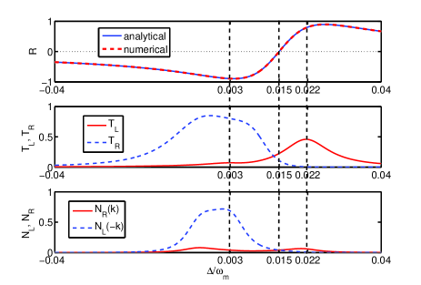
Figure 6: (Color online) The rectifying factor, transport efficiency and excitation number in cavity as a function of the driving detuning $\Delta$, here we set $\Delta_{L}=\Delta_{C}=\Delta$, $\Delta_{R}=\Delta+\Delta_{LR}$. Other parameters are $g/\omega_{m}=5\times 10^{-3}$, $\kappa/g=2$, $J_{L}/\omega_{m}=5\times 10^{-3}$, $J_{R}/\omega_{m}=5\times 10^{-3}$, $\Delta_{LR}/\omega_{m}=-2\times 10^{-2}$.

III.2 Single-photon source

Photon blockade effect allows only single-photon transmission through the system. Now, we show that our device can work as single-photon sources. The system is only driven from left or right cavity, i.e., $\varepsilon_{L}=\varepsilon$, $\varepsilon_{R}=\varepsilon_{C}=0$ or $\varepsilon_{R}=\varepsilon$, $\varepsilon_{L}=\varepsilon_{C}=0$, the mean occupation photon numbers

$$N_{R}(k) = N_{L}(-k)$$

$$= |\frac{J_{L}J_{R}\varepsilon}{J_{R}^{2}\alpha_{L}+\alpha_{R}(J_{L}^{2}-\alpha_{L}(\alpha_{C}+\delta))}|^{2}.$$

As shown in Fig.7, the system only allowed single-photon transport no matter the light from left or right when $g_{R}^{(2)}(k)\approx g_{L}^{(2)}(-k)\approx 0$. The transport efficiency $\mathcal{T}_{L}=\mathcal{T}_{R}\approx 0.5$, which means the output of system is single-photon state if the input is two-photon state. Under this condition, the device can control the single-photon transport in the channel or worked as a single-photon sources. This kind of device can only worked in strong coupling regime ($g/\kappa>1$) because there is no multi-path interference in output ports. We also notice that, $\mathcal{R}\equiv 0$ even if $\alpha_{L}\neq\alpha_{R},J_{L}\neq J_{R}$. In order to achieve rectification, requires $\varepsilon_{C}\neq 0$.

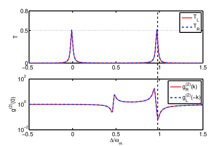
Figure 7: (Color online) The transport efficiency and second-order correlation of output ports as a function of the driving detuning $\Delta$, here we set $\Delta_{L}=\Delta_{R}=\Delta$, $\Delta_{C}=\Delta+\Delta_{LC}$. Other parameters are $g/\omega_{m}=0.2$, $J_{L}/\omega_{m}=0.1$, $J_{R}/\omega_{m}=0.1$, $\kappa/g=0.1$, $\Delta_{LC}/\omega_{m}=-1$.

III.3 Optomechanical optical capacitor

As we have shown in Fig. 4, the photons in left cavity exhibit antibunching although the directly nonlinear interaction only appear in OM cavity. Similar to the nonlinear shift $3\delta$ in OM cavity, the effective nonlinearity in cavity $L$ and $R$ can be equivalent to the resonance energy shift $\delta_{L}$ ($\delta_{R}$). If cavity $L$ and $R$ both appear photon antibunching effect due to the nonlinear shift and interference while the OM cavity appears photon bunching effect, when we drive the cavity $L$ and $R$, the photons can be stored in OM cavity. Reversing the process, one can release the photons.

As shown in Fig. 8(a) and (c), the system is a symmetric structure. The field from left and right cavity can be regarded as input ($+k$) of OM, meanwhile the field from OM cavity can be regarded as output ($-k$) of OM. In Fig. 8(b), when $\{\omega_{L},\omega_{R}\}>\omega_{D}$ and $\{\omega_{L},\omega_{R}\}>\omega_{C}$, i.e. $\{\Delta_{LC},\Delta_{RC}\}<0$, $\{\Delta_{L},\Delta_{R}\}>0$, the nonlinear frequency shift in left (right) cavity $\delta_{L}(\delta_{R})$ will enlarge the transition energy of two-photon excitation, which means the probability of two-photon state will be suppressed, the photon appears anti-bunching in cavity $L$ ($R$). At the same time, the nonlinear shift in OM cavity $3\delta$ will diminish the detuning between tunneling field $\omega_{L}$ ($\omega_{R}$) and resonance frequency $\omega_{C}$, the photon appears bunching in OM cavity. Especially for $\omega_{D}\approx\omega_{C}+3\delta$, OM cavity exhibit strong bunching due to the resonance absorption. Under this condition, the probability amplitude of photons in cavity OM will be much larger than in cavity $L$ and $R$, photons can be stored in OM cavity. Reversing the process, as shown in Fig. 8(d), when $\omega_{C}>\omega_{D}$ and $\omega_{C}>\{\omega_{L},\omega_{R}\}$, i.e. $\{\Delta_{LC},\Delta_{RC}\}>0$, $\Delta_{C}>0$, the nonlinear frequency shift $3\delta$ will enlarge the transition energy of two-photon excitation, the photon appears antibunching in OM cavity. Meanwhile, the nonlinear shift in left and right cavity $\delta_{L}$ and $\delta_{R}$ will diminish the detuning between tunneling field $\omega_{C}$ and resonance frequency $\{\omega_{L},\omega_{R}\}$, the photon appears bunching in left and right cavity. Under this condition, the photons can be released from OM cavity.

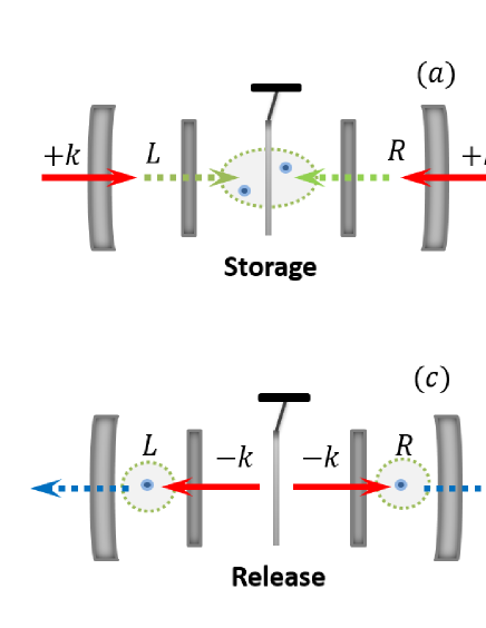
Figure 8: (Color Online) Pictorial representation and eigensystem of photon storage and release progress.

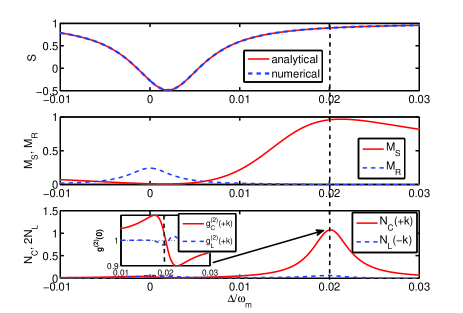
Figure 9: (Color online) The storage factor, storage-release efficiency and excitation number in cavity as a function of the driving detuning $\Delta$, here we set $\Delta_{L}=\Delta_{R}=\Delta$, $\Delta_{C}=\Delta+\Delta_{LC}$. Other parameters are $g/\omega_{m}=5\times 10^{-3}$, $\kappa/g=1$, $J_{L}/\omega_{m}=J_{R}/\omega_{m}=1\times 10^{-3}$, $\Delta_{LC}/\omega_{m}=-2\times 10^{-2}$.

In order to describe the characteristics of energy storage and release. We define the storage factor $\mathcal{S}$ and storage-release efficiency $\mathcal{M}$.

$$\mathcal{S} = \frac{Q_{C}[+k]-Q_{L}[-k]-Q_{R}[-k]}{Q_{C}[+k]+Q_{L}[-k]+Q_{R}[-k]},$$ (14)

$$\mathcal{M}_{S} = \frac{Q_{C}[+k]}{Q_{C}[+k]+Q_{L}[+k]+Q_{R}[+k]},$$ (15)

$$\mathcal{M}_{R} = \frac{Q_{L}[-k]+Q_{R}[-k]}{Q_{C}[-k]+Q_{L}[-k]+Q_{R}[-k]},$$ (16)

where $\mathcal{S}=+1$ indicates maximal storage with the enhanced transport to the OM cavity, $\mathcal{S}=0$ indicates no storage and release, while $\mathcal{S}=-1$ indicates maximal release with enhanced transport to the left and right cavities. $\mathcal{M}_{S}=1$ or $\mathcal{M}_{R}=1$ indicates the photons are totally stored in or released from OM cavity, respectively.

For simplicity, assume that all parameters of cavity $L$ and $R$ are exactly the same in the following discussion. The photon number of the two cavity $Q_{L}[+k]=Q_{R}[+k]$ and $Q_{L}[-k]=Q_{R}[-k]$. We discuss the storage effect shown in Fig. 9. When $\frac{\Delta}{\omega_{m}}$ is around $0.02$, $S\approx+1$ which indicates that system allows photon transfer into the OM cavity $L\rightarrow C\leftarrow R$ only, and the transfer is prohibited out from the OM cavity $L\leftarrow C\rightarrow R$, the photon number in cavity $L$ and $R$ from OM cavity approximately equal to zero. At this time, second-order correlation $g_{C}^{(2)}(0)>1$, photons appear bunching effect in OM cavity, and $g_{R}^{(2)}(0)=g_{L}^{(2)}(0)<1$, photons appear antibunching effect in left and right cavity. The convergence filed ($+k$) is bounded in OM cavity, system exhibits storage characteristic. As shown in Fig. 10, system exhibits release characteristic. When $\frac{\Delta}{\omega_{m}}$ is around $0.007$, $S\approx-1$ which indicates that system allows photon transfer out from OM cavity $L\leftarrow C\rightarrow R$ only. The second-order correlation $g_{C}^{(2)}(0)<1$, photons appear antibunching effect in OM cavity, and $g_{R}^{(2)}(0)=g_{L}^{(2)}(0)>1$, photons appear bunching effect in left and right cavity. That is, divergent filed ($-k$) is released from OM cavity. We also notice that, when $\mathcal{S}=1$ and $\mathcal{M}_{S}=1$, indicates complete storage, no matter the field from left or right cavity can be stored in OM cavity, which is similar to capacitor charge process. While, when $\mathcal{S}=-1$ and $\mathcal{M}_{R}=1$ indicates complete release, the field in OM cavity can be released through the left and right cavity completely, which is similar to capacitor discharge process. And the two progress can be controlled by the detuning of driving field $\Delta$. On the other hand, like filter effect, there is no photon in the channel at the frequency which let $\mathcal{S}=1$ and $\mathcal{M}_{S}=1$ (complete absorption), but have no effect of the frequency which let $\mathcal{S}=-1$ and $\mathcal{M}_{R}=1$ (complete release).

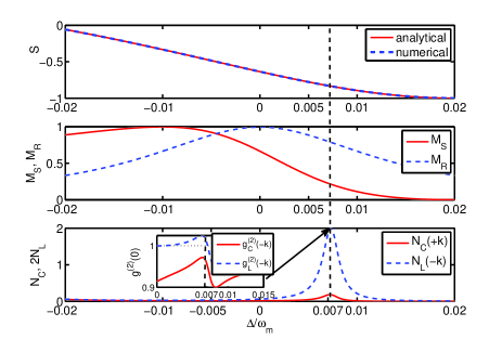
Figure 10: (Color online) The storage factor, storage-release efficiency and excitation number in cavity as a function of the driving detuning $\Delta$, here we set $\Delta_{L}=\Delta_{R}=\Delta$, $\Delta_{C}=\Delta+\Delta_{LC}$. Other parameters are $g/\omega_{m}=1\times 10^{-3}$, $\kappa/g=2$, $J_{L}/\omega_{m}=J_{R}/\omega_{m}=1\times 10^{-2}$, $\Delta_{LC}/\omega_{m}=2\times 10^{-2}$.

In the previous discussion, we ignore the effects of the mechanical thermal bath. Now, to investigate the influence of the mechanical thermal temperature on the correlation function, we include the mechanical thermal reservoir. Using master Eq.(4), in Fig. 11, we plot the minimum values of $g_{L}^{2}(0)$ as a function of the reservoir temperature, and the $g_{L}^{2}(0)$ versus $\frac{\Delta}{\omega_{m}}$ affected by the thermal reservoir are also displayed in the inset. When the temperature below $1$ $mk$ (marked with the shadow area), the thermal heating nearly have no effects in Fig. 11(a), because when the influence of the mechanical bath far below single-photon coupling rate, i.e. $\gamma n_{th}\ll g$, the bath effect can be ignored. With current experimental techniques, one can easily set $g/\gamma\gg 1$ EP1 ; EP2 , which means that a small value of phonon number $n_{th}$ can be tolerance with no much effects. Also, we can clearly see that the antibunching effect becomes more and more weaker with temperature increasing. In UPB regime, as shown in Fig. 11(b), the antibunching effect is more sensitive to the bath temperature. And this quantum effect will disappear when the temperature over $5$ $mK$ ($n_{th}=0.62$). Fortunately, the current experiment conditions of ground state cooling can achieve $n_{th}=0.34\pm 0.05$ FE1 . This provides some ability to against the quantum decoherence of our system. Even so, to maintain the antibunching effect, the mechanical thermal noise still needs to be suppressed.

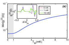
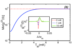
Figure 11: (Color online) The minimum equal-time second-order correlation $g_{L}^{(2)}(0)$ as a function of mechanical bath temperature $T_{M}$ with mechanical frequency $\omega_{m}=0.1GHz$ and dissipation rate $\gamma=1KHz$. Other parameters are (a) $\Delta_{L}=\Delta_{R}=\Delta_{C}$, $g/\omega_{m}=0.2$, $J_{L}=J_{R}=\omega_{m}/10$, $\kappa/\omega_{m}=10^{-2}$. (b) $\Delta_{L}=\Delta_{C}$, $\Delta_{LR}/\omega_{m}=0.1$, $g/\omega_{m}=10^{-2}$, $J_{L}/\omega_{m}=0.1$, $J_{R}/\omega_{m}=0.01$, $\kappa/g=1.3$.

IV conclusion

In this paper, we employ the radiation pressure and the destructive interference effects to construct the controller of photon transport. By coupling the an cavity optomechanical system to two cavities, we show that the photon blockade can be achieved both in strong and weak coupling regime. In strong coupling regime, the photon blockade effects is mainly resulted from the nonlinearity of radiation pressure in optomechanical cavity, while in weak coupling regime, the photon blockade effects is mainly because of the interference between multipath for two-photon excitation in cavities. For few photon control of one-dimensional transmission, the system can worked as optical diode without the requirement of the strength of radiation pressure strong coupling, and the rectification of photons can be controlled by the detuning of driving field $\Delta$. If we just drive the cavity from left or right cavity only, the system can function as single-photon source. Furthermore, when two fields transport into the OM cavity through the cavity $L$ and $R$, the device can store and release photons as a capacitor in appropriate parameter regime. These novel properties provide a promising application of optomechanical system in quantum information processing and quantum circuit realization.

Acknowledgments: The project was supported by NSFC under Grant No. 11074028

Appendix A solution of the probability amplitudes

We set $\kappa_{L}=\kappa_{R}=\kappa_{C}=\kappa$, $\omega_{m}\gg g$, adiabatically eliminate the degree of the oscillators, we can obtain the equations of motion of the probability amplitudes under weak pumping regime $C_{0}\gg C_{s1}\gg C_{s1s2}$. We drop higher-order terms in the zero- and one-photon probability amplitudes

$$i\dot{C_{L}} = \alpha_{L}C_{L}+\varepsilon_{L}C_{0}+J_{L}C_{C},$$

$$i\dot{C_{C}} = (\alpha_{C}+\delta)C_{C}+\varepsilon_{C}C_{0}+J_{L}C_{L}+J_{R}C_{R},$$

$$i\dot{C_{R}} = \alpha_{R}C_{R}+\varepsilon_{R}C_{0}+J_{R}C_{C},$$

$$i\dot{C_{LC}} = (\alpha_{L}+\alpha_{C}+\delta)C_{LC}+\varepsilon_{L}C_{C}+\varepsilon_{C}C_{L}+\sqrt{2}J_{L}(C_{LL}+C_{CC})+J_{R}C_{LR},$$

$$i\dot{C_{LR}} = (\alpha_{L}+\alpha_{R})C_{LR}+\varepsilon_{L}C_{R}+\varepsilon_{R}C_{L}+J_{L}C_{CR}+J_{R}C_{LC},$$

$$i\dot{C_{CR}} = (\alpha_{R}+\alpha_{C}+\delta)C_{CR}+\varepsilon_{C}C_{R}+\varepsilon_{R}C_{C}+\sqrt{2}J_{R}(C_{RR}+C_{CC})+J_{L}C_{LR},$$

$$i\dot{C_{LL}} = 2\alpha_{L}C_{LL}+\sqrt{2}\varepsilon_{L}C_{L}+\sqrt{2}J_{L}C_{LC},$$

$$i\dot{C_{CC}} = (2\alpha_{C}+4\delta)C_{CC}+\sqrt{2}\varepsilon_{C}C_{C}+\sqrt{2}J_{L}C_{LC}+\sqrt{2}J_{R}C_{CR},$$

$$i\dot{C_{RR}} = 2\alpha_{R}C_{RR}+\sqrt{2}\varepsilon_{R}C_{R}+\sqrt{2}J_{R}C_{CR},$$ (17)

where $\alpha_{L}=\Delta_{L}-i\kappa/2$, $\alpha_{R}=\Delta_{R}-i\kappa/2$, $\alpha_{C}=\Delta_{C}-\kappa/2+\delta$. If we set the initial state is vacuum state, i.e. $C_{0}(0)=1,C_{s1}(0)=C_{s1s2}(0)=0,\{s1,s2\}\in\{L,C,R\}$, In the weak-driving regime, $\{\varepsilon_{C}/\kappa_{C}$,$\varepsilon_{L}/\kappa_{L}$,$\varepsilon_{R}/\kappa_{R}\}\ll 1$, the photon number is small, so we have $C_{0}(\infty)\approx C_{0}(0)$, then the long-time solution of equations can be approximately obtained as,

$$C_{L} = \frac{[-J_{R}^{2}+\alpha_{R}(\alpha_{C}+\delta)]\varepsilon_{L}+J_{L}(-\alpha_{R}\varepsilon_{C}+J_{R}\varepsilon_{R})}{D_{1}},$$ (18)

$$C_{C} = \frac{\alpha_{L}\alpha_{R}\varepsilon_{C}-J_{L}\alpha_{R}\varepsilon_{L}-J_{R}\alpha_{L}\varepsilon_{R}}{D_{1}},$$ (19)

$$C_{R} = \frac{[-J_{L}^{2}+\alpha_{L}(\alpha_{C}+\delta)]\varepsilon_{R}+J_{R}(-\alpha_{L}\varepsilon_{C}+J_{L}\varepsilon_{L})}{D_{1}},$$ (20)

$$C_{LL} = \frac{C_{L}\sum_{j=(L,C,R)}l_{L,j}\varepsilon_{j}+J_{L}C_{C}\sum_{j=(L,C,R)}l_{C,j}\varepsilon_{j}+J_{L}J_{R}C_{R}\sum_{j=(L,C,R)}l_{R,j}\varepsilon_{j}}{\sqrt{2}D_{2}},$$ (21)

$$C_{CC} = \frac{J_{L}C_{L}\sum_{j=(L,C,R)}c_{L,j}\varepsilon_{j}+C_{C}\sum_{j=(L,C,R)}c_{C,j}\varepsilon_{j}+J_{R}C_{R}\sum_{j=(L,C,R)}c_{R,j}\varepsilon_{j}}{\sqrt{2}D_{2}},$$ (22)

$$C_{RR} = \frac{J_{L}J_{R}C_{L}\sum_{j=(L,C,R)}r_{L,j}\varepsilon_{j}+J_{R}C_{C}\sum_{j=(L,C,R)}r_{C,j}\varepsilon_{j}+C_{R}\sum_{j=(L,C,R)}r_{R,j}\varepsilon_{j}}{\sqrt{2}D_{2}},$$ (23)

where the first term in Eq. (A5) describes two-photon state generated by driving field in cavity $L$, the second term describes two-photon excitation due to photon tunneling between OM cavity and left cavity with coupling rate $J_{L}$, the third term describes two-photon excitation due to photon tunneling between right cavity and left cavity through the OM cavity, when the collective effect of this three progress let $C_{LL}\approx 0$, photons exhibit blockade effect in cavity $L$. As well as Eq. (A6) and (A7).

$$D_{1} = J_{L}^{2}\alpha_{L}+J_{R}^{2}\alpha_{R}-\alpha_{L}\alpha_{R}(\alpha_{C}+\delta),$$

$$D_{2} = \sum_{s=L,R}\alpha_{s}[J_{s}^{2}-\alpha_{s}(\alpha_{s}+\alpha_{C}+\delta)][2J_{s}^{2}(\alpha_{s}+\alpha_{C}+2\delta)-\alpha_{s}(\alpha_{s}+\alpha_{C}+\delta)(\alpha_{C}+2\delta)],$$

$$l_{L,L} = J_{L}^{4}\alpha_{R}+[J_{R}^{2}-(\alpha_{L}+\alpha_{R})(\alpha_{C}+\alpha_{L}+\delta)][-\alpha_{R}(\alpha_{C}+\alpha_{R}+\delta)(\alpha_{C}+2\delta)+J_{R}^{2}(\alpha_{C}+\alpha_{R}+2\delta)]$$

$$+J_{L}^{2}[J_{R}^{2}(\alpha_{L}-\alpha_{R})-\alpha_{R}(\alpha_{C}^{2}+\alpha_{R}(\alpha_{L}+\alpha_{R})+(3\alpha_{L}+\alpha_{R})\delta+2\delta^{2}+\alpha_{C}(2\alpha_{L}+\alpha_{R}+3\delta))],$$

$$l_{L,C} = J_{L}[J_{R}^{2}(\alpha_{L}+\alpha_{R})(\alpha_{C}+\alpha_{R}+2\delta)-\alpha_{R}(\alpha_{C}+2\delta)(-J_{L}^{2}+(\alpha_{L}+\alpha_{R})(\alpha_{C}+\alpha_{R}+\delta))],$$

$$l_{L,R} = J_{L}J_{R}[-J_{R}^{2}(\alpha_{C}+\alpha_{R}+2\delta)+\alpha_{R}(J_{L}^{2}+(\alpha_{C}+\alpha_{R}+\delta)(\alpha_{C}+2\delta))],$$

$$l_{C,L} = -J_{R}^{2}(\alpha_{L}+\alpha_{R})(\alpha_{C}+\alpha_{R}+2\delta)+\alpha_{R}(\alpha_{C}+2\delta)[-J_{L}^{2}+(\alpha_{L}+\alpha_{R})(\alpha_{C}+\alpha_{R}+\delta))],$$

$$l_{C,C} = J_{L}[J_{R}^{2}\alpha_{L}+J_{L}^{2}\alpha_{R}-\alpha_{R}(\alpha_{L}+\alpha_{R})(\alpha_{C}+\alpha_{R}+\delta)],$$

$$l_{C,R} = J_{L}J_{R}\alpha_{R}(\alpha_{C}+\alpha_{L}+\alpha_{R}+2\delta),$$

$$l_{R,L} = J_{R}^{2}(\alpha_{C}+\alpha_{R}+2\delta)-\alpha_{R}[J_{L}^{2}+(\alpha_{C}+\alpha_{R}+\delta)(\alpha_{C}+2\delta)],$$

$$l_{R,C} = J_{L}\alpha_{R}(\alpha_{C}+\alpha_{L}+\alpha_{R}+2\delta),$$

$$l_{R,R} = -J_{L}J_{R}(\alpha_{C}+\alpha_{L}+\alpha_{R}+2\delta),$$

$$c_{L,L} = J_{L}[J_{R}^{2}\alpha_{L}+J_{L}^{2}\alpha_{R}-\alpha_{R}(\alpha_{L}+\alpha_{R})(\alpha_{C}+\alpha_{R}+\delta)],$$

$$c_{L,C} = \alpha_{L}[-J_{R}^{2}\alpha_{L}-J_{L}^{2}\alpha_{R}+\alpha_{R}(\alpha_{L}+\alpha_{R})(\alpha_{C}+\alpha_{R}+\delta)],$$

$$c_{L,R} = J_{R}[J_{R}^{2}\alpha_{L}-\alpha_{R}(-J_{L}^{2}+\alpha_{L}(2\alpha_{C}+\alpha_{L}+\alpha_{R}+2\delta))],$$

$$c_{C,L} = J_{L}\alpha_{L}[-J_{R}^{2}\alpha_{L}-J_{L}^{2}\alpha_{R}+\alpha_{R}(\alpha_{L}+\alpha_{R})(\alpha_{C}+\alpha_{R}+\delta)],$$

$$c_{C,C} = -J_{L}^{4}\alpha_{R}-\alpha_{L}[J_{R}^{2}-(\alpha_{L}+\alpha_{R})(\alpha_{C}+\alpha_{L}+\delta)][J_{R}^{2}-\alpha_{R}(\alpha_{C}+\alpha_{R}+\delta)]$$

$$+J_{L}^{2}[-J_{R}^{2}(\alpha_{L}+\alpha_{R})+\alpha_{R}(\alpha_{L}^{2}+\alpha_{C}(2\alpha_{L}+\alpha_{R})+\alpha_{R}(\alpha_{R}+\delta)+\alpha_{L}(\alpha_{R}+2\delta))],$$

$$c_{C,R} = J_{R}\alpha_{R}[-J_{R}^{2}\alpha_{L}-J_{L}^{2}\alpha_{R}+\alpha_{L}(\alpha_{L}+\alpha_{R})(\alpha_{C}+\alpha_{L}+\delta)],$$

$$c_{R,L} = J_{L}[J_{R}^{2}\alpha_{L}-\alpha_{R}(-J_{L}^{2}+\alpha_{L}(2\alpha_{C}+\alpha_{L}+\alpha_{R}+2\delta))],$$

$$c_{R,C} = \alpha_{R}[-J_{R}^{2}\alpha_{L}-J_{L}^{2}\alpha_{R}+\alpha_{L}(\alpha_{L}+\alpha_{R})(\alpha_{C}+\alpha_{L}+\delta)],$$

$$c_{R,R} = J_{R}[J_{R}^{2}\alpha_{L}+J_{L}^{2}\alpha_{R}-\alpha_{L}(\alpha_{L}+\alpha_{R})(\alpha_{C}+\alpha_{L}+\delta)],$$

$$r_{i,j} = l_{i,j}(J_{L}\leftrightarrow J_{R},\alpha_{L}\leftrightarrow\alpha_{R}),(i,j=\{L,C,R\})$$ (24)

The second order correlation functions with zero time-delay are

$$g_{L}^{(2)}(0) = \frac{2|C_{LL}|^{2}}{(|C_{L}|^{2}+|C_{LC}|^{2}+|C_{LR}|^{2}+2|C_{LL}|^{2})^{2}}$$

$$\approx \frac{2|C_{LL}|^{2}}{|C_{L}|^{4}},$$

$$g_{C}^{(2)}(0) = \frac{2|C_{CC}|^{2}}{(|C_{C}|^{2}+|C_{LC}|^{2}+|C_{CR}|^{2}+2|C_{CC}|^{2})^{2}}$$

$$\approx \frac{2|C_{CC}|^{2}}{|C_{C}|^{4}},$$

$$g_{R}^{(2)}(0) = \frac{2|C_{RR}|^{2}}{(|C_{R}|^{2}+|C_{CR}|^{2}+|C_{LR}|^{2}+2|C_{RR}|^{2})^{2}}$$ (25)

$$\approx \frac{2|C_{RR}|^{2}}{|C_{R}|^{4}}.$$

The mean occupation numbers of three cavities are

$$N_{L} = (|C_{L}|^{2}+|C_{LC}|^{2}+|C_{LR}|^{2}+2|C_{LL}|^{2})N_{0}$$

$$\approx |C_{L}|^{2}N_{0},$$

$$N_{C} = (|C_{C}|^{2}+|C_{LC}|^{2}+|C_{CR}|^{2}+2|C_{CC}|^{2})N_{0}$$

$$\approx |C_{C}|^{2}N_{0},$$

$$N_{R} = (|C_{R}|^{2}+|C_{CR}|^{2}+|C_{LR}|^{2}+2|C_{RR}|^{2})N_{0}$$ (26)

$$\approx |C_{R}|^{2}N_{0},$$

where $N_{0}=(\varepsilon_{L}/\kappa_{L})^{2}+(\varepsilon_{C}/\kappa_{C})^{2}+(\varepsilon_{R}/\kappa_{R})^{2}$.

References

- (1) K. Stannigel, P. Komar, S. J. M. Habraken, S. D. Bennett, M. D. Lukin, P. Zoller, and P. Rabl, Phys. Rev. Lett. 109, 013603 (2012).
- (2) A. Miranowicz, M. Paprzycka, Y. X. Liu, J. Bajer, and F. Nori, Phys. Rev. A 87, 023809 (2013).
- (3) X. -W. Xu and Y. Li, Phys. Rev. A 90, 033832 (2014).
- (4) H.-Z. Wu, Z.-B. Yang, and S.-B. Zheng, Phys. Rev. A 82, 034307 (2010).
- (5) Y. Han, B. He, K. Heshami, C.-Z. Li, and C. Simon, Phys. Rev. A 81, 052311 (2010).
- (6) F.-Y. Hong and S.-J. Xiong, Phys. Rev. A 78, 013812 (2008).
- (7) J. L. O Brien, Science 318, 1567 (2007).
- (8) H. A. Haus, Waves and Fields in Optoelectronics (Prentice-Hall, Englewood Cliffs, NJ, 1984).
- (9) K. Gallo, G. Assanto, K. Parameswaran, and M. Fejer. Appl. Phys. Lett. 79, 314 (2001).
- (10) B. E. A. Saleh and M. C. Teich, Fundamentals of Photonics, 2nd ed. (Wiley, New York, 2007).
- (11) L. Fan, J. Wang, L. T. Varghese, H. Shen, B. Niu, Y. Xuan, A. M. Weiner, and M. Qi, Science. 335, 447 (2011).
- (12) M. S. Kang, A. Butsch, and P. S. J. Russell, Nat. Photon 5, 549 (2011).
- (13) D.-W. Wang, H.-T. Zhou, M.-J. Guo, J.-X. Zhang, J. Evers, and S.-Y. Zhu, Phys. Rev. Lett. 110, 093901 (2013).
- (14) E. Mascarenhas, D. Gerace, D. Valente, S. Montangero, A. Auff ves, and M. F. Santos, Europhysics Lett. 106, 54003 (2014).
- (15) H. Z. Shen, Y. H. Zhou, and X. X. Yi, Phys. Rev. A 90, 023849 (2014).
- (16) P. Rabl, Phys. Rev. Lett. 107, 063601 (2011).
- (17) T. Ramos, V. Sudhir, K. Stannigel, P. Zoller, and T. J. Kippenberg, Phys. Rev. Lett. 110, 193602 (2013).
- (18) G. S. Agarwal and S. Huang, Phys. Rev. A 81, 041803 (2010).
- (19) J. D. Teufel, D. Li, M. S. Allman, K. Cicak, A J. Sirois, J. D. Whittaker, and R. W. Simmonds, Nature (London) 471, 204 (2011).
- (20) S. Aldana, C. Bruder, and A. Nunnenkamp, Phys. Rev. A 88, 043826 (2013).
- (21) L. Zhou, J. Cheng, Y. Han, and W. Zhang, Phys. Rev. A 88, 063854 (2013).
- (22) J. D. Teufel, T. Donner, D. Li, J. W. Harlow, M. S. Allman, K. Cicak, A J. Sirois, J. D. Whittaker, K. W. Lehnert, and R. W. Simmonds, Nature (London)475, 359 (2011).
- (23) J. Chan, T. P. M. Alegre, A. H. Safavi-Naeini, J. T. Hill, A. Krause, S. Gröblacher, M. Aspelmeyer, and O. Painter, Nature (London)478, 89 (2011).
- (24) B. Abbott et al., New J. Phys. 11, 073032 (2009).
- (25) A. Pontin, M. Bonaldi, A. Borrielli, F. S. Cataliotti, F. Marino, G. A. Prodi, E. Serra, and F. Marin, Phys. Rev. A 89, 023848 (2014).
- (26) M. Aspelmeyer, T. J. Kippenberg, and F. Marquardt, Rev. Mod. Phys. 86, 1391 (2014).
- (27) W. Z. Jia and Z. D. Wang, Phys. Rev. A 88, 063821 (2013).
- (28) X. X. Ren, H. K. Li, M. Y. Yan, Y. C. Liu, Y. F. Xiao, and Q. Gong, Phys. Rev. A 87, 033807 (2013).
- (29) J.-Q. Liao and F. Nori, Phys. Rev. A 88, 023853 (2013).
- (30) X.-Y. Lü, W.-M. Zhang, S. Ashhab, Y. Wu, and F. Nori, Sci. Rep. 3, 2943 (2013).
- (31) D. Hu, S.-Y. Huang, J.-Q. Liao, L. Tian, and H.-S. Goan, Phys. Rev. A 91, 013812 (2015).
- (32) M. Bamba, A. Imamoǧlu, I. Carusotto, and C. Ciuti, Phys. Rev. A 83, 021802 (2011).
- (33) C. W. Gardner and P. Zoller, Quantum Noise (Springer, Berlin, 2000).
- (34) T. C. H. Liew and V. Savona, Phys. Rev. Lett. 104, 183601 (2010).
- (35) X.-W. Xu and Y. Li, Phys. Rev. A 90, 043822 (2014).
- (36) K. W. Murch, K. L. Moore, S. Gupta, and D. M. Stamper-Kurn, Nat. Phys. 4, 561 (2008).
- (37) D. Kleckner, B. Pepper, E. Jeffrey, P. Sonin, S. M. Thon, and D. Bouwmeester, Opt. Express 19, 19708 (2011).