Probing (topological) Floquet states through DC transport

Abstract

We consider the differential conductance of a periodically driven system connected to infinite electrodes. We focus on the situation where the dissipation occurs predominantly in these electrodes. Using analytical arguments and a detailed numerical study we relate the differential conductances of such a system in two and three terminal geometries to the spectrum of quasi-energies of the Floquet operator. Moreover these differential conductances are found to provide an accurate probe of the existence of gaps in this quasi-energy spectrum, being quantized when topological edge states occur within these gaps. Our analysis opens the perspective to describe the intermediate time dynamics of driven mesoscopic conductors as topological Floquet filters.

1 Introduction

Recently, the possibility to induce an out-of-equilibrium topological state of matter through irradiation or a periodic driving has stimulated numerous works. While initially the external driving perturbation was used to trigger a phase transition between states of conventional topological order [1, 2, 3], fascinating topological properties specific to driven out-of-equilibrium states were soon identified [4, 5, 6]. While several proposals to realize and probe these topological states in various artificial systems have turned out to be successful [7, 8, 9, 10, 11, 12, 13, 14]. Their realization in condensed matter have proved to be challenging [15, 16].

There is a strong analogy between equilibrium topological insulators and topological driven states. Both require the existence of a gap in the spectrum characterizing their single particle states: topological insulators are band insulators with a gap in the energy spectrum of the single particle Hamiltonian while topological driven states have a gap in the spectrum of the Floquet operator. In both cases, a nontrivial topology manifests itself through the appearance within this gap of robust states located at the edge of the system. However, while in an insulator the gap separates empty states from occupied states, the thermodynamics of gapped periodically driven states is much less understood. Recent studies have stressed the differences between the nature of the states reached at long time in such periodically driven systems and the equilibrium ground states of insulators [17, 18, 19, 20].

Here we follow a different route: we focus on the relation between the DC transport of a periodically driven system and its quasi-energy Floquet spectrum in a regime where the times of flight of electrons through the system are shorter than the characteristic inelastic scattering times, which can be the case in mesoscopic systems. This provides a way to avoid the issue of long time dynamics of driven systems, which was raised in recent studies [19, 20, 21]. Technically, this requires that the dominant perturbation of the unitary evolution of the driven system is the presence of the electrodes: dissipation should occur in the leads. From this point of view, the driven system behaves as a topological Floquet filter instead of an out-of-equilibrium steady-state analogue of an equilibrium insulating state.

DC transport is known to be an ideal probe of the existence of edge states in topological equilibrium phases realized in condensed matter, particularly in two dimensions. In a seminal paper [22] Markus Büttiker demonstrated how the non-local conductances in a Hall bar fully characterize the nature of the quantum Hall effect and the associated chiral edge states. This approach was recently extended to study the quantum spin Hall effect occuring in HgTe/CdTe quantum wells [23, 24]. In this time-reversal invariant topological phase, the existence of a Kramers pair of counter-propagating edge states leads to a series of non-local conductances whose experimental observation clearly identified this new phase. For topological driven systems, the situation is more confusing: building on earlier works on the transport through a topological periodically driven state [25, 3], recent studies have focused on the transport through a one-dimensional topological superconducting state [26], the effect on transport of the competition between heating by the drive and the coupling to the leads [21] or the quantization of conductances of a topological phase in multi-terminal geometry [27]. It was also proposed to probe quasienergy spectra (and topological edge states) through magnetization measurements [28] and tunneling spectroscopy [29]. However, the relation between transport and the existence of topological edge states in periodically driven states remains unclear, and a summation procedure over different energies in the lead was proposed to recover a quantized conductance [26, 30]. The purpose of our paper is to reconsider the relation between the (non-local) differential conductances of periodically driven systems and their Floquet quasi-energy spectrum, allowing for a direct relation between these differential conductances and the topological indices associated with the spectral gaps. In particular we will establish a protocol in a multi-terminal geometry allowing for this identification. In this point of view, a topological periodically driven system is viewed as a topological Floquet filter with selective edge transport occurring for specific voltage biases between a lead and the system. These voltage biases lead to a stationnary DC current by counterbalancing the time dependence of Floquet states.

2 From Floquet theory to scattering theory

2.1 Floquet theory for open systems

We consider a periodically driven quantum system connected to $N_{\text{leads}}$ equilibrium electrodes through good contacts with large transmissions. The system is described by a Hamiltonian $\hat{H}^{\text{sys}}(t)-\hat{\Sigma}$ where $\hat{H}^{\text{sys}}(t+T)=\hat{H}^{\text{sys}}(t)$ with $T$ the period of the drive, and $\hat{\Sigma}$ is a self-energy accounting for the coupling between the system and its environment (e.g. the leads). We assume in the following that this self-energy is dominated by the exchange with the electrons in the leads. When all characteristic times of the leads are small with respect to the characteristic times of the system, we can use the so-called wide band approximation [31] where the self-energy is assumed to be constant in energy: $\hat{\Sigma}(E)\simeq\hat{\Sigma}$. The dynamics of the system is described by the evolution operator $\hat{U}(t,t^{\prime})$ which obeys the equation

$$\mathrm{i}\hbar\frac{\mathrm{d}}{\mathrm{d}t}\hat{U}(t,t^{\prime})=\left(\hat{H}^{\text{sys}}(t)-\hat{\Sigma}\right)\hat{U}(t,t^{\prime}).$$ (1)

Of great importance is the Floquet operator which is the evolution operator after one period $\hat{U}(T,0)$. When diagonalizable, it can be decomposed on the left eigenstates $\bra{\tilde{\phi}_{\alpha}}$ and the right eigenstates $\ket{\tilde{\phi}_{\alpha}}$ of $\hat{U}(T,0)$

$$\begin{split}\hat{U}(T,0)\ket{\phi_{\alpha}}&=\lambda_{\alpha}\ket{\phi_{\alpha}},\\ \bra{\tilde{\phi}_{\alpha}}\hat{U}(T,0)&=\lambda_{\alpha}\bra{\tilde{\phi}_{\alpha}},\end{split}$$ (2)

that constitute a bi-orthonormal basis of the Hilbert space

$$\braket{\tilde{\phi}_{\alpha}\mid\phi_{\beta}}=\delta_{\alpha\beta}\ ;\ \sum_{\alpha}\ket{\phi_{\alpha}}\bra{\tilde{\phi}_{\alpha}}=\text{Id}.$$ (3)

The eigenvalues $\lambda_{\alpha}$ in Eq. (2) are called the Floquet multiplicators and read

$$\lambda_{\alpha}=\exp\left[-\mathrm{i}\left(\frac{\varepsilon_{\alpha}}{\hbar}-\mathrm{i}\gamma_{\alpha}\right)T\right].$$ (4)

The coefficient $\varepsilon_{\alpha}$ is called the quasienergy and $\gamma_{\alpha}$ is its damping rate whose inverse gives the life-time of the eigenstate. Note that the quasienergy being a phase, it is defined modulo the driving frequency $\omega=2\pi/T$. Any state at arbitrary time $t$ can then be constructed from the eigenstates of the Floquet operator. It is particularly useful to define the left and right Floquet states

$$\begin{split}\ket{u_{\alpha}(t)}&=\mathrm{e}^{\mathrm{i}\left(\varepsilon_{\alpha}/\hbar-\mathrm{i}\gamma_{\alpha}\right)t}\ \hat{U}(t,0)\ket{\phi_{\alpha}},\\ \bra{\tilde{u}_{\alpha}(t)}&=\mathrm{e}^{-\mathrm{i}\left(\varepsilon_{\alpha}/\hbar-\mathrm{i}\gamma_{\alpha}\right)t}\ \bra{\tilde{\phi}_{\alpha}}\hat{U}(0,t),\end{split}$$ (5)

which are periodic in time, $\ket{u_{\alpha}(t)}=\ket{u_{\alpha}(t+T)}$ (same for $\bra{\tilde{u}_{\alpha}(t)}$), so that they can be expanded in Fourier series

$$\begin{split}\ket{u_{\alpha}(t)}&=\sum_{p\in\mathbb{Z}}\mathrm{e}^{-\mathrm{i}p\omega t}\ket{u_{\alpha}^{(p)}},\\ \bra{\tilde{u}_{\alpha}(t)}&=\sum_{p\in\mathbb{Z}}\mathrm{e}^{\mathrm{i}p\omega t}\bra{\tilde{u}_{\alpha}^{(p)}},\end{split}$$ (6)

where the harmonics read

$$\begin{split}\ket{u_{\alpha}^{(p)}}=\frac{1}{T}\int_{0}^{T}\mathrm{d}t\;\mathrm{e}^{\mathrm{i}p\omega t}\ket{u_{\alpha}(t)}\\ \bra{\tilde{u}_{\alpha}^{(p)}}=\frac{1}{T}\int_{0}^{T}\mathrm{d}t\;\mathrm{e}^{-\mathrm{i}p\omega t}\bra{\tilde{u}_{\alpha}(t)}.\end{split}$$ (7)

From Eqs. (3) and (5) the evolution operator can be expanded on the Floquet states as

$$\hat{U}(t,t^{\prime})=\sum_{\alpha}\mathrm{e}^{-\mathrm{i}\left(\varepsilon_{\alpha}/\hbar-\mathrm{i}\gamma_{\alpha}\right)\left(t-t^{\prime}\right)}\ket{u_{\alpha}(t)}\bra{\tilde{u}_{\alpha}(t^{\prime})}.$$ (8)

This expression can finally be decomposed on the harmonics of the Floquet states by using Eq.(6)

$$\!\!\!\!\hat{U}(t,t^{\prime})=\!\!\!\sum_{\begin{subarray}{c}\alpha\\ p,p^{\prime}\in\mathbb{Z}\end{subarray}}\!\!\!\mathrm{e}^{-\mathrm{i}\left[\left(\frac{\varepsilon_{\alpha}}{\hbar}-\mathrm{i}\gamma_{\alpha}\right)(t-t^{\prime})+\omega(pt-p^{\prime}t^{\prime})\right]}\ket{u_{\alpha}^{(p)}}\!\bra{\tilde{u}_{\alpha}^{(p^{\prime})}}.$$ (9)

In practice, the spectrum of Floquet operator of the semi-infinite system can be obtained numerically either by direct a computation of $U(T,0)$ (e.g. as a discretized in time version of the infinite product) or through its representation in Sambe space [32].

2.2 Differential conductance

Based on a standard formalism, we can calculate analytically the differential conductance of the periodically driven system in a multi-terminal geometry and relate it to the quasienergy spectrum of the system. We follow the standard Floquet scattering formalism [33, 31, 34, 35, 26, 27] to describe the transport properties of this multiterminal setup in a phase coherent regime. We consider the rolling average over a period $T$ (all time-averages in the following are also rolling averages over one driving perdiod) of the current entering each lead labelled by the index $\ell$:

$$\mathcal{I}_{\ell}(t)=\frac{1}{T}\int_{t}^{t+T}\mathrm{d}t^{\prime}\;\braket{\hat{J}_{\ell}(t^{\prime})}.$$ (10)

where $\braket{\hat{J}_{\ell}(t^{\prime})}$ is the expectation value of the current entering lead $\ell$ at time $t^{\prime}$. This average current satisfies a relation [33, 31, 34]:

$$\mathcal{I}_{\ell}(t)=\frac{e}{h}\int\mathrm{d}E\;\sum_{\ell^{\prime}\neq\ell}\left[T_{\ell\ell^{\prime}}(t,E)f_{\ell^{\prime}}(E)-T_{\ell^{\prime}\ell}(t,E)f_{\ell}(E)\right],$$ (11)

where $f_{\ell}(E)$ is the Fermi-Dirac distribution of the lead $\ell$ assumed to be at equilibrium at the chemical potential $\mu_{\ell}$. The $T_{\ell\ell^{\prime}}(E)$ are the time-averaged transmission coefficients between lead $\ell$ and $\ell^{\prime}$ which will be discussed below. We define the differential conductance $G_{\ell\ell^{\prime}}(t,E)$ as the sensitivity of the current entering the lead $\ell$ to variations of the chemical potential $\mu_{\ell^{\prime}}$ of the lead $\ell^{\prime}$ :

$$G_{\ell\ell^{\prime}}(t,E)\equiv-e\left.\frac{\mathrm{d}\mathcal{I}_{\ell}}{\mathrm{d}\mu_{\ell^{\prime}}}\right|_{\mu_{\ell^{\prime}}=\mu_{\text{sys}}+E}.$$ (12)

Note that this definition is not symmetric in the various chemical potentials $\mu_{\ell}$, as opposed to other definitions used in the literature. In the long time stationary regime on which we focus, $t\to\infty$, the average conductances $G_{\ell\ell^{\prime}}(t,E)$ are expected to reach a value independent on the choice of origin of time $t$ and associated initial conditions [31], which we denote by $G_{\ell\ell^{\prime}}^{\infty}(E)$.

We obtain from Eq. (11) the zero temperature time-averaged differential conductances

$$G_{\ell\ell^{\prime}}^{\infty}(E) =\frac{e^{2}}{h}T_{\ell\ell^{\prime}}(E)\qquad\text{for $\ell\neq\ell^{\prime}$}$$ (13)

$$G_{\ell\ell}^{\infty}(E) =-\frac{e^{2}}{h}\sum_{\ell^{\prime}\neq\ell}T_{\ell^{\prime}\ell}(E),$$ (14)

which satisfy the rule $\sum_{\ell}G_{\ell,\ell^{\prime}}(E)=0$ for any $\ell^{\prime}$ (the average current leaving the system is independent on the chemical potentials in the leads). This formula is analogous to the Landauer-Büttiker formula for the differential conductance of multiterminal equilibrium systems.

2.3 Generalized Fisher-Lee relations

The average transmission coefficients $T_{\ell\ell^{\prime}}(E)$ can be related to the Floquet-Green functions of the system, in a way analogous to the case of undriven conductors [36]. The retarded Green functions in mixed energy-time representations are defined by

$${\hat{\mathcal{G}}}(t,E)=\frac{1}{\mathrm{i}\hbar}\int d\tau\ e^{\mathrm{i}E\tau/\hbar}\,\hat{\cal G}(t,t-\tau)$$ (15)

where $\hat{\cal G}(t,t^{\prime})$ satisfies

$$\begin{split}\left(\mathrm{i}\hbar\frac{\mathrm{d}}{\mathrm{d}t}-\hat{H}^{\text{sys}}(t)+\hat{\Sigma}\right)\hat{\cal G}(t,t^{\prime})=\delta(t-t^{\prime}).\end{split}$$ (16)

It is related to the evolution operator defined in Eq.(1) by

$${\hat{\cal G}}(t,t^{\prime})=\frac{1}{\mathrm{i}\hbar}\Theta(t-t^{\prime})\hat{U}(t,t^{\prime}).$$ (17)

From the decomposition Eq.(9) of $\hat{U}(t,t^{\prime})$ over the harmonics of the Floquet states, we express the Floquet-Green functions

$$\hat{\mathcal{G}}^{(p)}(E)=\frac{1}{T}\int_{0}^{T}\mathrm{d}t\;\mathrm{e}^{\mathrm{i}p\omega t}\,{\mathcal{G}}(t,E).$$ (18)

as

$$\hat{\mathcal{G}}^{(p)}(E)=\sum_{r,\alpha}\frac{\ket{u_{\alpha}^{(p+r)}}\bra{\tilde{u}_{\alpha}^{(r)}}}{E-\left[\varepsilon_{\alpha}+r\hbar\omega-\mathrm{i}\hbar\gamma_{\alpha}\right]}.$$ (19)

The transmission coefficients are expressed as

$$T_{\ell^{\prime}\ell}(E)=\sum_{p\in\mathbb{Z}}T_{\ell^{\prime}\ell}^{(p)}(E),$$ (20)

where each $T^{(p)}_{\ell^{\prime}\ell}(E)$ is the transmission coefficient for an electron injected in lead $\ell$ at the energy $E=\mu_{\ell}$ and leaving the system in lead $\ell^{\prime}$ at the energy $E+p\hbar\omega$, i.e. after having exchanged $p$ quanta with the driving perturbation. They read (see A and [31, 34, 35, 37]):

$$T_{\ell^{\prime}\ell}^{(p)}(E)=\text{Tr}\left[\hat{\mathcal{G}}^{{\dagger}(p)}(E)\hat{\Gamma}_{\ell^{\prime}}(E+p\hbar\omega)\hat{\mathcal{G}}^{(p)}(E)\hat{\Gamma}_{\ell}(E)\right]$$ (21)

where $\hat{\Gamma}_{\ell}(E)$ is the coupling operator at energy $E$ between the system and the electrode $\ell$.

Note that when the rates $\gamma_{\alpha}$ are sufficiently small for the quasi-energies $\epsilon_{\alpha}$ occurring in Eq. (19) to be “well-defined”, the equations (19,20,21) imply that the transmission coefficient $T_{\ell^{\prime}\ell}(E))$ and thus the differential conductance $G_{\ell^{\prime}\ell}(E)$ vanishes whenever the energy $\mu_{\ell}=E$ does not correspond to a quasi-energy $\epsilon_{\alpha}$ up to a multiple of $\hbar\omega$. This is nothing but the conservation of energy of incident state which holds modulo $\hbar\omega$ in a periodically driven system. This property allows one to probe the existence of gaps in the quasi-energy spectrum of the Floquet operator. Note however that to access the whole quasi-energy spectrum, the lead $\mu_{\ell}$ has to be strongly biased (with a bias of order $\hbar\omega$) with respect to the scattering region at $\mu_{\text{sys}}$, a situation far from the standard procedure to probe equilibrium phases, but required to probe an inherently out-of-equilibrium Floquet state. Moreover, in the presence of a ballistic mode connecting two leads $\ell$ and $\ell^{\prime}$ such as the edge mode of a topological Floquet state, we expect the corresponding $T_{\ell^{\prime}\ell}(E)$ to be quantized provided both interfaces are sufficiently transparent. Note however that as the states leaving the systems have component of energies $E+p\hbar\omega$, this implies a perfect transparency over a broad range of energies. These two properties allow for a potential probe of topological Floquet states through non-local transport. In the next section, we study this application by a numerical implementation of transport through an AC driven system.

3 Numerical study

In the following, we provide numerical evidence of the correspondence between the differential conductance and the quasi-energy spectrum in a periodically driven system. In particular, we show that a single out-of-equilibrium topological edge state corresponds to a quantized differential conductance. The chirality of these topological edge states is probed in a multi-terminal setup.

3.1 Model and method

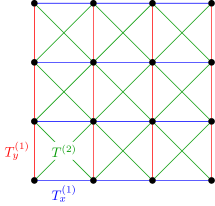
Figure 1: Lattice of couplings for the half-BHZ model with two orbitals per site of the square lattice. Blue and red links correspond to the $T^{(1)}_{x}$ and $T^{(1)}_{y}$ nearest neighbor coupling matrices between $s$ and $p$ orbitals while the green links represent $T^{(2)}$ the second-nearest neighbor coupling matrix.

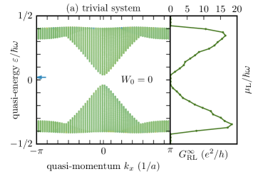
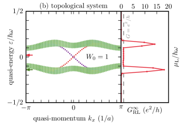
Figure 2: Quasi-energy spectrum of the driven half-BHZ model in an infinitely long ribbon and corresponding asymptotic two terminal differential conductance $G_{\text{RL}}^{\infty}(E)$ for finite system connected to infinite leads. The results are shown for parameters with only trivial gaps with driving amplitude $F=2$ (Left) and a topological gap at $\epsilon=0$ or $F=8$ (Right). The quasi-energy spectra are obtained for strip of width $W=$60$$ sites by diagonalization in Sambe space with $5$ sidebands. The quasi-energies $\varepsilon$ are shown in units of the driving frequency $\hbar\omega$ as a function of the quasi-momentum in the direction of the ribbon $k_{x}$. For the topological case ($F=$8.0$$, Right figure), states appear inside the gap $\epsilon=0$, located on either side of the ribbon. The location of each Floquet mode was numerically computed and converted to a color using the color scale of figure 3. Delocalized states (and states located in the bulk) are in green, whereas states located on an edge are in red or blue, depending on which edge. This signals the appearance of a topologically non-trivial gap around $\epsilon=0$. On the other hand, the gaps in $\epsilon=\pm\hbar\omega/2$ remains topologically trivial in both cases. The asymptotic long time limit of the corresponding two-terminal differential conductance is displayed as a function of the chemical potential of the left lead (black dots and lines) for a finite sample of size $W\times L=$60$\times$30$$ sites. This differential conductance $G_{\text{RL}}^{\infty}$ is quantized, with $G=1e^{2}/h$ in the topological quasi-energy gap (Right) and vanishes in the trivial gap (Left). Hence it is an accurate probe of the existence of topological gap in the quasi-energy spectrum of open conductors connected to electrodes. The colored arrows indicate the chemical potential of the incoming lead used in the computations of Fig. 4.

Figure 3: Geometry of the semi-infinite system used to compute quasi-energy spectra of figure 2. In those spectra, the color of each point represents the average $y$ position of the corresponding Floquet mode, according to the color scale shown on this figure.

Following [5], we use the restriction to spins up of the Bernevig-Hugues-Zhang model of quantum spin Hall effect in HgTe/CdTe quantum wells [38] (referred to as half-BHZ model). As the Haldane model [39] it realizes an anomalous quantum Hall equilibrium phase, but on a square lattice with two orbitals per site, denoted $s$ and $p$. The tight-binding Hamiltonian with nearest and next-to-nearest neighbors hoppings (see Fig. 1) can therefore be written as a two-by-two matrix on the $(s,p)$ basis as

$$\begin{split}&H_{\text{BHZ}}=\sum_{x,y}\biggl{[}\left[\left(M-J-4B\right)\sigma_{z}-\mu\sigma_{0}\right]\ket{x,y}\bra{x,y}\\ &+T^{(1)}_{x}\ket{x,y}\bra{x+1,y}+T^{(1)}_{y}\ket{x,y}\bra{x,y+1}\\ &+T^{(2)}\left(\ket{x,y}\bra{x+1,y+1}+\ket{x,y}\bra{x+1,y-1}\right)\biggr{]}\\ &+\text{h.c.}\end{split}$$ (22)

with hopping matrices

$$\begin{split}T^{(1)}_{x/y}=\ \frac{A}{2\mathrm{i}}\sigma_{x/y}+B\sigma_{z}\text{ and }T^{(2)}=\frac{J}{4}\sigma_{z}\end{split}$$ (23)

where $\sigma_{x,y,z}$ are the Pauli matrices and $\sigma_{0}$ the identity matrix. The parameters of this Hamiltonian are chosen as $M=$-1.0$$, $J=$1.5$$, $A=$4.0$$, $B=$1.5$$ : they correspond to an equilibrium phase which is a trivial insulator. A topological insulating phase can be reached by varying e.g. $M$ such that $0<M/B<4$ or $4<M/B<8$. This trivial equilibrium phases is submitted to a periodic on-site perturbation [5]

$$\Delta H(t)=\sum_{x,y}F\left[\sin(\omega t)\sigma_{x}+\cos(\omega t)\sigma_{y}\right]\ket{x,y}\bra{x,y}.$$ (24)

Note that this perturbation does not correspond to the variation of a parameter of the initial Hamiltonian. Throughout our study, we have used a driving frequency $\omega=$20$$. Depending on the strength $F$, this perturbation can drive the system either towards a topologically nontrivial out-of-equilibrium state or in a topologically trivial out-of-equilibrium state. We have chosen two values $F=2$ and $F=8$ of the driving amplitude so that gaps open at $\epsilon=0,\pm\hbar\omega/2$ of the quasi-energy spectrum. For each value of $F$ and each gap, we have computed numerically the bulk topological invariant $W_{\varepsilon}[U]$ associated to the quasi-energy gap around $\epsilon$ [5] to ensure that $F=2$ correspond to a trivial gapped Floquet state, while $F=8$ corresponds to a topological gapped Floquet state with a non-trivial gap at $\epsilon=0$. Alternatively, in the two cases we have computed the quasi-energy spectrum for the driven model in an infinitely long ribbon of width $W=$60$$ sites (see Fig. 3) by diagonalization in Sambe space with $5$ sidebands. The resulting spectra are shown in Fig. 2: they show as expected that states located at each edge on the ribbon appear inside the $\epsilon=0$ gap for the topological case ($F=8$) as opposed to the trivial case ($F=2$).

Finally, to study transport through the system, leads are attached to a finite size system. These leads are modeled by a simple tight-binding Hamiltonian on a square lattice with nearest neignbors hoppings with amplitude $J_{0}=$8$$. An onsite potential is added to the lead Hamiltonian to reduce mismatches between the incoming and outgoing states of the leads and the scattering states of the central region.

The numerical calculations are performed using the numerical method described in [35]. Although the technique is based on wavefunctions, it is mathematically equivalent to the Green function approach used in this article (see Eq. (49) of [35] for the connection with the transmission coefficient as well as section 5.4 for the link with Floquet theory). Our implementation is based on the Kwant package [40].

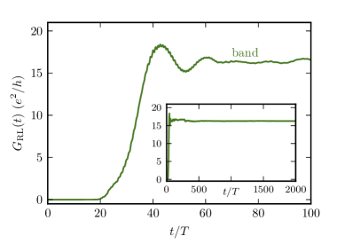
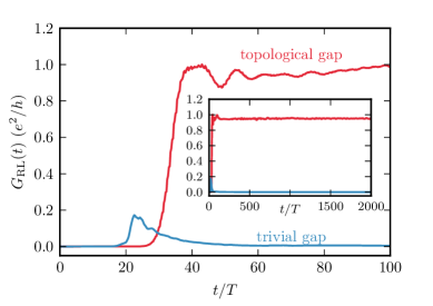
Figure 4: Two-terminal differential conductance as a function of time, in the transient regime, for two chemical potentials, in a topologically trivial case. Green curve: incoming chemical potential in a quasi-energy band ; blue and red curves: incoming chemical potential in the bulk quasi-energy gap, in a trivial (blue) and a topological (red) case. Inset: longer simulations were carried out to ensure convergence. The asymptotic value is denoted by $G_{\text{RL}}^{\infty}$.

3.2 Probing the quasi-energy bands and gaps through two-terminal differential conductance

The differential conductance $G_{\text{RL}}(t)$ is computed in a two-terminal setup through a sample of width $W=60$ and length $L=$30$$ sites. Throughout this study, the chemical potential of the undriven system was chosen as $\mu_{\text{sys}}=0$. To get rid of oscillations faster than the driving frequency, which are irrelevant for our purpose, we perform a sliding average over one driving period $T$. After a transient regime, the (averaged) differential conductance $\bar{G}(t)$ converges to a finite value (see Fig. 4). This transient regime can be understood as the time of flight of the state injected at the left lead to the right lead after the driving perturbation has been turned on and the Floquet states developed inside the system. When the chemical potential of the incoming lead lies in a topological quasi-energy gap of the scatterng region, transport occurs through a chiral state localized near the edge of the sample. We can easily evaluate the travel length $L$. The expected group velocity is extracted from the slope of the quasi-energy dispersion relation from Fig. 2 through

$$v_{\text{g}}=\frac{1}{\hbar}\frac{\mathrm{d}\varepsilon}{\mathrm{d}k},$$ (25)

and we obtain $v_{\text{g}}=$0.15(1)$\,a\omega$ where $a$ is the lattice spacing and $\omega$ the driving frequency. This correlates perfectly with the time $\Delta t$ of the first increase from zero of the conductance from the switching on of the driving field. From the curve on Fig. 4 we find find $L/\Delta t=$0.14(1)$\,a\omega$.

After this transient regime, the differential conductance $G_{\text{RL}}(t)$ reaches a long time stationary limit $G_{\text{RL}}^{\infty}$, as shown in the inset of Fig. 4. As expected, this asymptotic differential conductance is sensitive to the quasi-energy spectrum of the driven system: when in a spectral band, it reaches high values but vanishes when the chemical potential $\mu_{\text{L}}-\mu_{\text{sys}}$ lies in a trivial spectral gap of the Floquet operator, as shown on the left plot of Fig. 4. Moreover, when this spectral gap is topological, the associated presence of chiral states at the edge of the system shown in Fig. 2 (Right) leads to a quantized two terminal conductance as shown in the right plot of Fig. 4. To further study the correlation between the differential conductance as a function of the chemical potential $\mu_{\text{L}}-\mu_{\text{sys}}=E$ and the spectral gap of the system we have studied the behavior of the long time limit of this conductance as a function of $E$. The corresponding results as well the spectra of the isolated driven models are plotted in Fig. 2 for both the trivial and a topological gapped Floquet states. We find a strong correlation between the vanishing of both quantities for the topologically trivial case: the differential conductance vanishes only inside a trivial gap, except at the edge of the gap where finite size effects occurs due to imperfect transparencies of the contact with the leads, as shown on a magnified view around the gap $\epsilon=0$ in Fig. 5. This demonstrates both that the quasi-energy spectrum of the finite system connected to infinite leads is sufficiently close to the spectrum of the isolated infinite strip, and that the differential conductance is an accurate probe of this spectrum for the open system. Moreover, in the topological case the asymptotic differential conductance remains constant equal to the number $n=1$ of edge states (in units of $e^{2}/h$) inside the topological gap as shown in Fig. 5. The small deviations from $G_{\text{RL}}^{\infty}=1\,e^{2}/h$ visible in figure 5 are attributed to the finite dispersion relation of the leads, which does not completely satisfy the wide band approximation and leads to imperfect transparencies of the contacts.

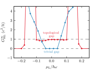
Figure 5: Zoom of Fig. 2 : asymptotic two-terminal differential conductance $G_{\text{RL}}^{\infty}$ in units of $e^{2}/h$ with respect to the chemical potential of the left lead (black dots and lines) around the quasi-energy gap $\epsilon=0$ for a trivial (red) and topological gap (red). The reference energy $\mu_{\text{L}}=0$ corresponds to an unbiased lead whose chemical potential identifies with the one of the driven system $\mu_{\text{sys}}=0$. The differential conductance vanishes in the quasi-energy gaps for a trivial spectral gap, but reaches an approximately constant and quantized value $G=e^{2}/h$ within the topological gap with one chiral edge mode. Deviations from $G_{\text{RL}}^{\infty}=1\,e^{2}/h$ are attributed to the finite dispersion relation of the leads, which does not completely satisfy the wide band approximation and leads to imperfect transparencies of the contacts.

3.3 Multiterminal geometry

A crucial characteristics of the edge states occurring in the topological gap of the spectrum shown in Fig. 2 (Right) is their chiral nature. In the equilibrium case this property together with their ballistic propagation leads to quantized conductance in a Hall bar geometry [39]. To test the chirality of the topological edge states, we have computed differential conductances in a three-terminal geometry shown in Fig.  6, where the width of the contact with the electrodes is $W=$30$$ sites, the total length (between $L$ and $R$ contacts) is $50$ sites, corresponds to all three arms having a length of $10$ sites. In this geometry, we monitor the two differential conductances

$$\begin{split}G_{R,T}(E)=-e\left.\frac{\mathrm{d}\mathcal{I}_{R}}{\mathrm{d}\mu_{T}}\right|_{\mu_{T}=\mu_{\text{sys}}+E},\\ G_{L,T}(E)=-e\left.\frac{\mathrm{d}\mathcal{I}_{L}}{\mathrm{d}\mu_{T}}\right|_{\mu_{T}=\mu_{\text{sys}}+E}.\end{split}$$ (26)

where $\mathcal{I}_{R,L}$ are the current in the $R,L$ contacts averaged over one period $T$ of drive (see eq. 10). The chemical potential of the system is still set to $\mu_{\text{sys}}=0$ (as if imposed e.g. by a backgate).

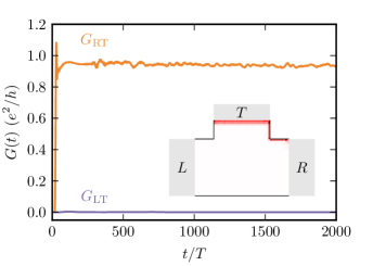
Figure 6: Three-terminal differential conductance $G_{\text{LT}}$ (violet) and $G_{\text{RT}}$ (orange) as a function of time for a chemical potential of the top lead in a topological bulk gap. After an initial transient regime, asymptotic values for the nonlocal conductances are reached with $G_{\text{LT}}^{\infty}=$0.0002(1)$\,e^{2}/h$ and $G_{\text{RT}}^{\infty}=$0.94(1)$\,e^{2}/h$. The simultaneous vanishing of $G_{\text{LT}}^{\infty}$ and quantized $G_{\text{RT}}^{\infty}$ to the two-terminal value demonstrates the chiral nature of topological edge states. This is further illustrated in the inset by the corresponding probability density $|\psi(t,x)|^{2}$ in the stationnary regime (here at $t=1000\ T$) which is entirely localized around the $T\to R$ edge, demonstrating furthermore the high transparency of the $R$ contact for this edge mode. Simulations are done with a width of the contacts $W=$30$$ sites and a total length of $50$ sites.

We consider the case of a topological gap round $\epsilon=0$ (see Fig. 2 (Right)). First we set the chemical potential of the top lead inside this gap ($\mu_{T}=0$). The time evolution of the differential conductances are shown in Fig. 6. After a transient regime, the differential conductances converge to asymptotic values $G_{\text{LT}}^{\infty}=$0.0002(1)$\,e^{2}/h$ and $G_{\text{RT}}^{\infty}=$0.94(1)$\,e^{2}/h$. The value of $G_{\text{LT}}^{\infty}$ is in agreement with the two terminal results, while the vanishing of $G_{\text{RT}}^{\infty}$ is in perfect agreement with the chiral nature of the edge state moving clockwise for the chosen parameters. This can be contrasted with the case of a chemical potential $\mu_{T}=0$ set inside a bulk Floquet band, displayed in Fig. 7.

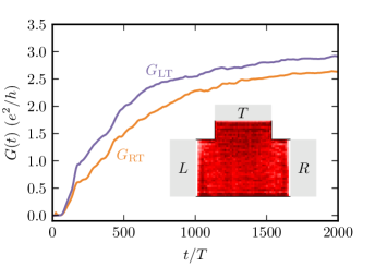
Figure 7: Three-terminal differential conductance $G_{\text{LT}}$ (violet) and $G_{\text{RT}}$ (orange) as a function of time for a chemical potential of the top lead in a quasi-energy band. A longer transient regime is observed, in agreement with smaller group velocities than for the edge states, and large asymptotic values for both $G_{\text{LT}}$ and $G_{\text{RT}}$ are reached, confirming the non-chiral nature of the corresponding Floquet states. The inset shows color map representing the probability density $|\psi(t,x)|^{2}$ for at $t/T=1800$, demonstrating the delocalized nature of the Floquet states.

In this case, after a longer transient regime due to slower group velocities, both conductances converge towards large finite values, confirming the absence of chirality for these bulk states.

Finally, to illustrate the spatial structure of these Floquet states we show in insets of Fig. 6 and 7 a color map of the probability density of the states reached at large times for both the topological gap and inside the bulk bands. The chiral nature of the states injected in the top lead is clearly apparent and confirms the transport results.

4 Discussion

We have studied the differential conductances $G_{\ell^{\prime}\ell}(E)$ defined in Eq. (12) for both a two-terminal and a three-terminal geometry. As for equilibrium phases, we have found that these conductances probe the topological nature of a gapped Floquet state: it vanishes whenever the chemical potential $\mu_{\ell}$ lies in a topologically trivial gap while we found it to be quantized for chemical potential inside a topological gap of quasi-energies. Moreover, the chiral nature of the edge states reflected on the value of the multi-terminal differential conductances within this gap. These results validate the relation between the DC transport through a periodically driven system and the Floquet description of the dynamics of the isolated system. This requires that the dissipation occurs mostly inside the leads, i.e. that the system is small enough for the travel times through it to be small compared with times scales of other source of dissipation (phonons, photons, etc). In that situation, the differential conductance of the system depends on the intermediate time evolution of the driven system and can be accurately described starting from the unitary dynamics of the driven system and its associated topological properties [5, 6]. This should be the case as long as phase coherence is preserved on the length scale of the sample, even in the presence of dissipation or weak interactions. This result paves the way towards a direct engineering of a topological filter through the implementation of Floquet states.

Our results on the quantization of differential conductances inside a topological gap contrast with some of the recent results on similar systems [26, 27, 30], where a summation procedure over multiple chemical potentials was required to recover a quantized conductance. Note that these previous results used a different measuring scheme of differential conductance, symmetric in chemical potentials of electrodes, which may filter out some of the energies of the outgoing electronic states, and thus require a summation protocol. In our case, a strong and asymmetric voltage bias is used to compensate the time dependence (through quasi-energies) of the Floquet states. Moreover, we have used in our numerical study a model with a single edge mode located around $k\simeq 0$ as opposed to double-mode topological gaps used previously. More complex edge structures may well lead to lower transparency of the interfaces for energies in the gap, and thus non-quantized conductances. The study of the transparency of such interface between a strongly driven conductor and a DC electrode is a deep and topical subject whose discussion goes beyond the scope of the present study.

Acknowledgments: This paper is dedicated to the memory of Markus Büttiker whose pioneering works on mesoscopic systems and in particular on scattering theory of chiral edge channels shaped our understanding of electronic transport. P.D. will always be grateful to him for his trust, enthusiasm and advice he received during his stay as a post-doc assistant in the Büttiker’s group. This work was supported by the French Agence Nationale de la Recherche (ANR) under grants SemiTopo (ANR-12-BS04-0007), IsoTop (ANR-10-BLAN-0419) and TopoDyn (ANR-14-ACHN-0031) and by the European Research Council grant MesoQMC (ERC-2010-StG_20091028 257241).

Appendix A Transmission coefficients

In the following, we extend the approach of [31] to a quasi-unidimensional system in the geometry of Fig. 3. The purpose is to describe the scattering through a two dimensional driven system, viewed as a Chern Floquet filter. We follow closely the derivation of [31] and only highlight the differences due to the geometry considered.

We consider a system composed of a central region $\mathcal{R}$ (the scattering region), which is submitted to a periodic excitation. This region is described by a time-periodic (with period $T=2\pi/\omega$) tight-binding Hamiltonian

$$H_{\text{sys}}=\sum_{nn^{\prime}\in\mathcal{R}}H_{nn^{\prime}}(t)c_{n}^{\dagger}c_{n^{\prime}}$$ (27)

with $H_{nn^{\prime}}(t+T)=H_{nn^{\prime}}(t)$, where $c_{n}$ is the annihilation operator of an electron in an localized state $n$ of the tight-binding model, the index $n$ representing the position on the Bravais lattice as well as internal degrees of freedom (sublattice, orbital, spin, etc.). This central region is connected to $N_{\text{leads}}$ leads described by the Hamiltonian

$$H_{\text{leads}}=\sum_{\ell=1}^{N_{\text{leads}}}\sum_{q\alpha}E_{\ell q\alpha}c_{\ell q\alpha}^{\dagger}c_{\ell q\alpha},$$ (28)

where $\alpha$ labels transverse modes of the semi-infinite lead and $q$ is the longitudinal momentum in this lead. We assume that the wavefunctions in the leads read

$$\psi_{\alpha q}(x,y)=\frac{1}{\sqrt{L}}\mathrm{e}^{-\mathrm{i}qx}\chi_{\alpha}(y),$$ (29)

and in particular that transverse modes $\ket{\chi}$ do not depend on $q$ and constitute an orthonormal basis of the transverse Hilbert space,. (Notice that this is not always the case, especially when a magnetic field is present [40]). The annihilation operator of a state localized at transverse position $y=y_{\ell}(n)$ in the interface with the lead  $\ell$ is written as

$$c_{\ell,y=y_{\ell}(n)}=\sum_{q\alpha}c_{\ell q\alpha}\chi_{\ell\alpha}^{*}(n).$$ (30)

The internal degrees of freedom in the leads can be taken into account, if needed, by considering more leads.

The contacts between the central region and the leads are described by the Hamiltonian

$$H_{\text{contacts}}=\sum_{\ell=1}^{N_{\text{leads}}}\sum_{n\in\mathcal{M}_{\ell}}\sum_{q}V_{\ell}c_{\ell,y=y_{\ell}(n)}^{\dagger}c_{n}+\text{h.c.}$$ (31)

where $\mathcal{M}_{\ell}$ describes the set of sites of the central region at the interface with lead $\ell$. In terms of the transverse modes creation/annihilation operators, this Hamiltonian reads

$$H_{\text{contacts}}=\sum_{\ell=1}^{N_{\text{leads}}}\sum_{n\in\mathcal{M}_{\ell}}\sum_{q\alpha}V_{\ell}\chi_{\ell\alpha}^{*}(n)c_{\ell q\alpha}^{\dagger}c_{n}+\text{h.c.}.$$ (32)

Using the approach of [31] which amounts to describe the correlations of the driven system in terms of the equilibrium noise in the leads, we obtain the equation (11) of main text with transmission coefficients

$$T_{\ell\ell^{\prime}}^{(p)}(E)=\!\!\!\!\sum_{\begin{subarray}{c}m,n\in\mathcal{I}_{\ell}\\ m^{\prime},n^{\prime}\in\mathcal{I}_{\ell^{\prime}}\end{subarray}}(\mathcal{G}_{mm^{\prime}}^{(p)}(E))^{*}\Gamma^{\ell}_{mn}(E+p\hbar\omega)\mathcal{G}_{nn^{\prime}}^{(p)}(E)\Gamma^{\ell^{\prime}}_{n^{\prime}m^{\prime}}(E),$$

that can be written as a trace on the interfaces (Eq. (21) of main text),

$$T_{\ell\ell^{\prime}}^{(p)}(E)=\text{Tr}\left[[\mathcal{G}^{(p)}(E)]^{\dagger}\Gamma^{\ell}(E+p\hbar\omega)\mathcal{G}^{(p)}(E)\Gamma^{\ell^{\prime}}(E)\right]$$

where

$$\Gamma_{\ell}(E)=2\pi\sum_{q\alpha}\left|V_{\ell}\right|^{2}\ket{\chi_{\alpha}}\!\bra{\chi_{\alpha}}\delta(E-E_{\ell q\alpha}).$$ (33)

This expression is in agreement with previous approaches based on different formalisms [34, 35, 37].

References

- Inoue and Tanaka [2010] J.-I. Inoue, A. Tanaka, Photoinduced Transition between Conventional and Topological Insulators in Two-Dimensional Electronic Systems, Phys. Rev. Lett. 105 (2010) 017401. doi:10.1103/PhysRevLett.105.017401.
- Lindner et al. [2011] N. H. Lindner, G. Refael, V. Galitski, Floquet topological insulator in semiconductor quantum wells, Nature Physics 7 (2011) 490–495. doi:10.1038/nphys1926. arXiv:1008.1792.
- Kitagawa et al. [2011] T. Kitagawa, T. Oka, A. Brataas, L. Fu, E. Demler, Transport properties of nonequilibrium systems under the application of light: Photoinduced quantum Hall insulators without Landau levels, Phys. Rev. B 84 (2011) 235108. doi:10.1103/PhysRevB.84.235108.
- Kitagawa et al. [2010] T. Kitagawa, E. Berg, M. Rudner, E. Demler, Topological characterization of periodically driven quantum systems, Phys. Rev. B 82 (2010) 235114. doi:10.1103/PhysRevB.82.235114. arXiv:1010.6126.
- Rudner et al. [2013] M. S. Rudner, N. H. Lindner, E. Berg, M. Levin, Anomalous Edge States and the Bulk-Edge Correspondence for Periodically Driven Two-Dimensional Systems, Phys. Rev. X 3 (2013) 031005. doi:10.1103/PhysRevX.3.031005. arXiv:1212.3324.
- Carpentier et al. [2015] D. Carpentier, P. Delplace, M. Fruchart, K. Gawedzki, Topological index for periodically driven time-reversal invariant 2D systems, Phys. Rev. Lett. 114 (2015) 106806. doi:10.1103/PhysRevLett.114.106806.
- Fang et al. [2012] K. Fang, Z. Yu, S. Fan, Realizing effective magnetic field for photons by controlling the phase of dynamic modulation, Nature Photonics 6 (2012) 782. doi:10.1038/nphoton.2012.236.
- Kitagawa et al. [2012] T. Kitagawa, M. A. Broome, A. Fedrizzi, M. S. Rudner, E. Berg, I. Kassal, A. Aspuru-Guzik, E. Demler, A. G. White, Observation of topologically protected bound states in photonic quantum walks, Nature Communications 3 (2012). doi:10.1038/ncomms1872. arXiv:1105.5334.
- Hauke et al. [2012] P. Hauke, O. Tieleman, A. Celi, C. Ölschläger, J. Simonet, J. Struck, M. Weinberg, P. Windpassinger, K. Sengstock, M. Lewenstein, A. Eckardt, Non-Abelian Gauge Fields and Topological Insulators in Shaken Optical Lattices, Phys. Rev. Lett. 109 (2012) 145301. doi:10.1103/PhysRevLett.109.145301.
- Rechtsman et al. [2013] M. C. Rechtsman, J. M. Zeuner, Y. Plotnik, Y. Lumer, D. Podolsky, F. Dreisow, S. Nolte, M. Segev, A. Szameit, Photonic Floquet topological insulators, Nature 496 (2013) 196–200. doi:10.1038/nature12066. arXiv:1212.3146.
- Hu et al. [2015] W. Hu, J. C. Pillay, K. Wu, M. Pasek, P. P. Shum, Y. D. Chong, Measurement of a Topological Edge Invariant in a Microwave Network, Phys. Rev. X 5 (2015) 011012. doi:10.1103/PhysRevX.5.011012.
- Karzig et al. [2014] T. Karzig, C.-E. Bardyn, N. Lindner, G. Refael, Topological polaritons from quantum wells in photonic waveguides or microcavities, 2014. arXiv:1406.4156.
- Reichl and Mueller [2014] M. D. Reichl, E. J. Mueller, Floquet edge states with ultracold atoms, Phys. Rev. A 89 (2014) 063628. doi:10.1103/PhysRevA.89.063628.
- Jotzu et al. [2014] G. Jotzu, M. Messer, R. Desbuquois, M. Lebrat, T. Uehlinger, D. Greif, T. Esslinger, Experimental realisation of the topological Haldane model, 2014. arXiv:1406.7874.
- Wang et al. [2013] K. H. Wang, H. Steinberg, P. Jarillo-Herrero, N. Gedik, Observation of Floquet-Bloch States on the Surface of a Topological Insulator, Science 342 (2013) 453.
- Onishi et al. [2014] Y. Onishi, Z. Ren, M. Novak, K. Segawa, Y. Ando, K. Tanaka, Instantaneous Photon Drag Currents in Topological Insulators, 2014. arXiv:1403.2492.
- Lazarides et al. [2014] A. Lazarides, A. Das, R. Moessner, Equilibrium states of generic quantum systems subject to periodic driving, Phys. Rev. E 90 (2014) 012110. doi:10.1103/PhysRevE.90.012110.
- Dehghani et al. [2014] H. Dehghani, T. Oka, A. Mitra, Dissipative Floquet Topological Systems, Phys. Rev. B 90 (2014) 195429. doi:10.1103/PhysRevB.90.195429.
- Iadecola et al. [2015] T. Iadecola, T. Neupert, C. Chamon, Occupation of topological Floquet bands in open systems, Phys. Rev. B 91 (2015) 235133. doi:10.1103/PhysRevB.91.235133.
- Seetharam et al. [2015] K. I. Seetharam, C.-E. Bardyn, N. H. Lindner, M. S. Rudner, G. Refael, Controlled Population of Floquet-Bloch States via Coupling to Bose and Fermi Baths, 2015. arXiv:1502.02664.
- Dehghani et al. [2015] H. Dehghani, T. Oka, A. Mitra, Out-of-equilibrium electrons and the Hall conductance of a Floquet topological insulator, Phys. Rev. B 91 (2015) 155422. doi:10.1103/PhysRevB.91.155422.
- Büttiker [1988] M. Büttiker, Absence of backscattering in the quantum Hall effect in multiprobe conductors, Phys. Rev. B 38 (1988) 9375. doi:10.1103/PhysRevB.38.9375.
- Roth et al. [2009] A. Roth, C. Brüne, H. Buhmann, L. W. Molenkamp, J. Maciejko, X.-L. Qi, S.-C. Zhang, Nonlocal Transport in the Quantum Spin Hall State, Science 325 (2009) 294. doi:10.1126/science.1174736.
- Büttiker [2009] M. Büttiker, Edge-State Physics Without Magnetic Fields, Science 325 (2009) 278–279. doi:10.1126/science.1177157.
- Gu et al. [2011] Z. Gu, H. A. Fertig, D. P. Arovas, A. Auerbach, Floquet Spectrum and Transport through an Irradiated Graphene Ribbon, Phys. Rev. Lett. 107 (2011) 216601. doi:10.1103/PhysRevLett.107.216601.
- Kundu and Seradjeh [2013] A. Kundu, B. Seradjeh, Transport Signatures of Floquet Majorana Fermions in Driven Topological Superconductors, Phys. Rev. Lett. 111 (2013) 136402. doi:10.1103/PhysRevLett.111.136402.
- Torres et al. [2014] L. E. F. F. Torres, P. M. Perez-Piskunow, C. A. Balseiro, G. Usaj, Multiterminal Conductance of a Floquet Topological Insulator, Phys. Rev. Lett. 113 (2014) 266801. doi:0.1103/PhysRevLett.113.266801.
- Dahlhaus et al. [2015] J. P. Dahlhaus, B. M. Fregoso, J. E. Moore, Magnetization Signatures of Light-Induced Quantum Hall Edge States, Phys. Rev. Lett. 114 (2015) 246802. URL: http://link.aps.org/doi/10.1103/PhysRevLett.114.246802. doi:10.1103/PhysRevLett.114.246802.
- Fregoso et al. [2014] B. M. Fregoso, J. P. Dahlhaus, J. E. Moore, Dynamics of tunneling into nonequilibrium edge states, Phys. Rev. B 90 (2014) 155127. URL: http://link.aps.org/doi/10.1103/PhysRevB.90.155127. doi:10.1103/PhysRevB.90.155127.
- Farrell and Pereg-Barnea [2015] A. Farrell, T. Pereg-Barnea, Edge State Transport in Floquet Topological Insulators, 2015. arXiv:1505.05584.
- Kohler et al. [2005] S. Kohler, J. Lehmann, P. Hanggi, Driven quantum transport on the nanoscale, Physics Reports 406 (2005) 379–443. doi:10.1016/j.physrep.2004.11.002.
- Sambe [1973] H. Sambe, Steady States and Quasienergies of a Quantum-Mechanical System in an Oscillating Field, Phys. Rev. A 7 (1973) 2203–2213. doi:10.1103/PhysRevA.7.2203.
- Moskalets and Büttiker [2002] M. Moskalets, M. Büttiker, Floquet scattering theory of quantum pumps, Phys. Rev. B 66 (2002) 205320. doi:10.1103/PhysRevB.66.205320.
- Stefanucci et al. [2008] G. Stefanucci, S. Kurth, A. Rubio, E. K. U. Gross, Time-dependent approach to electron pumping in open quantum systems, Phys. Rev. B 77 (2008) 075339. doi:10.1103/PhysRevB.77.075339.
- Gaury et al. [2013] B. Gaury, J. Weston, M. Santin, M. Houzet, C. Groth, X. Waintal, Numerical simulations of time-resolved quantum electronics, Physics Reports 534 (2013) 1. doi:10.1016/j.physrep.2013.09.001.
- Fisher and Lee [1981] D. S. Fisher, P. A. Lee, Relation between conductivity and transmission matrix, Phys. Rev. B 23 (1981) 6851(R). doi:10.1103/PhysRevB.23.6851.
- Arrachea and Moskalets [2006] L. Arrachea, M. Moskalets, Relation between scattering-matrix and Keldysh formalisms for quantum transport driven by time-periodic fields, Phys. Rev. B 74 (2006) 245322. doi:10.1103/PhysRevB.74.245322.
- Bernevig et al. [2006] B. A. Bernevig, T. L. Hughes, S.-C. Zhang, Quantum Spin Hall Effect and Topological Phase Transition in HgTe Quantum Wells, Science 314 (2006) 1757–1761. doi:10.1126/science.1133734. arXiv:cond-mat/0611399.
- Haldane [1988] F. D. M. Haldane, Model for a Quantum Hall Effect without Landau Levels: Condensed-Matter Realization of the "Parity Anomaly", Phys. Rev. Lett. 61 (1988) 2015–2018. doi:10.1103/PhysRevLett.61.2015.
- Groth et al. [2014] C. W. Groth, M. Wimmer, A. R. Akhmerov, X. Waintal, Kwant: a software package for quantum transport, New J. Phys 16 (2014) 063065. doi:10.1088/1367-2630/16/6/063065.