Removal of Curtaining Effects by a Variational Model with Directional Forward Differences
Abstract
Focused ion beam (FIB) tomography provides high resolution volumetric images on a micro scale. However, due to the physical acquisition process the resulting images are often corrupted by a so-called curtaining or waterfall effect. In this paper, a new convex variational model for removing such effects is proposed. More precisely, an infimal convolution model is applied to split the corrupted 3D image into the clean image and two types of corruptions, namely a striped part and a laminar one. As regularizing terms different direction dependent first and second order differences are used to cope with the specific structure of the corruptions. This generalizes discrete unidirectional total variational (TV) approaches. A minimizer of the model is computed by well-known primal dual techniques. Numerical examples show the very good performance of our new method for artificial and real-world data. Besides FIB tomography, we have also successfully applied our technique for the removal of pure stripes in Moderate Resolution Imaging Spectroradiometer (MODIS) data.
1 Introduction
The motivation for the present work was the analysis of aluminum matrix composites reinforced with silicon carbide particles by given high resolution 3D FIB tomography images.
FIB tomography, also known as serial sectioning, is an imaging technique, that has been used commercially for about years. It is applied for preparation and direct observation of structural cross-sections and the generation of microstructural data in three dimensions. While classical -ray tomography does often not reach the required material resolution, FIB tomography enables to investigate structures on a scale down to several nanometers.
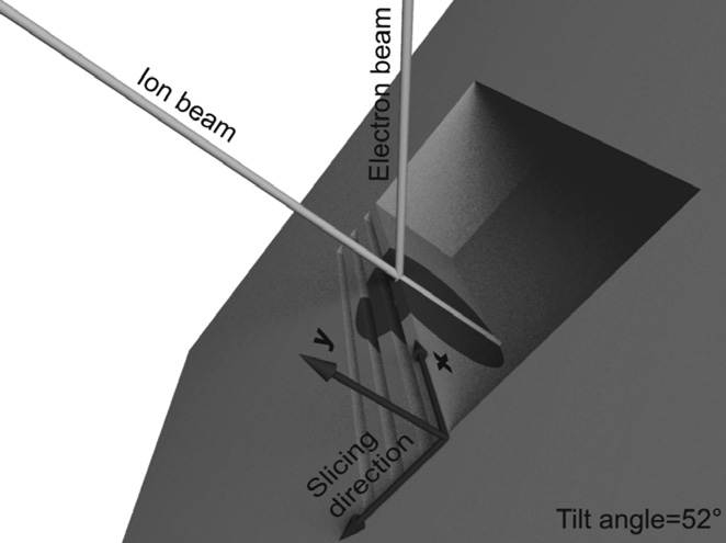
The FIB system combines a classical scanning electron microscope with an ion beam. An illustration is shown in Fig. 1. The ion beam mills and polishes the material sectionally, while the electron beam is used for imaging the surface after each section. Several hundred of these serial slices finally form a 3D image. For a more detailed introduction to FIB tomography we refer to [6, 20, 29].
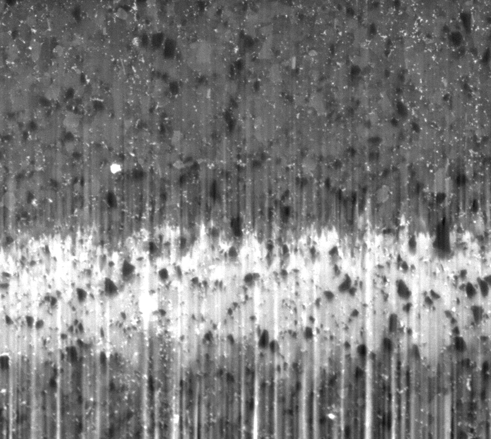
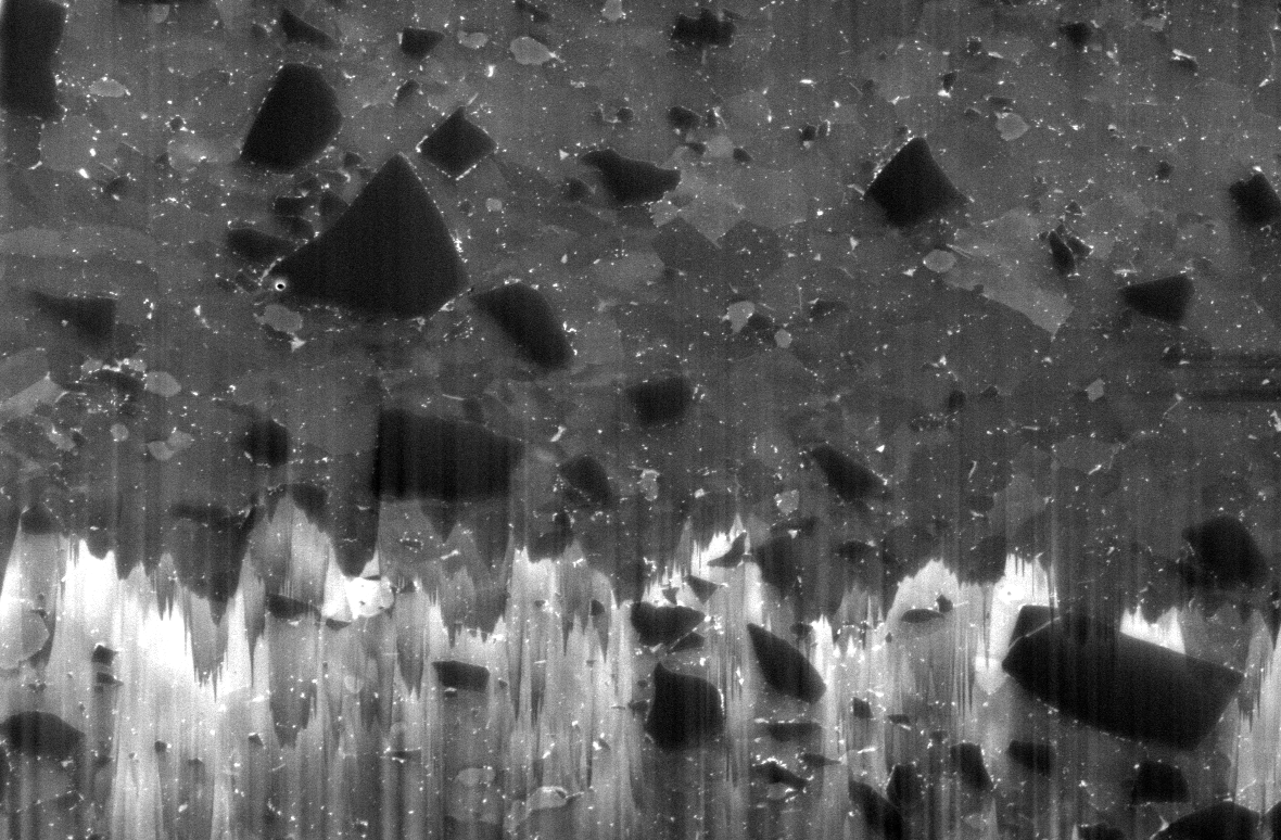
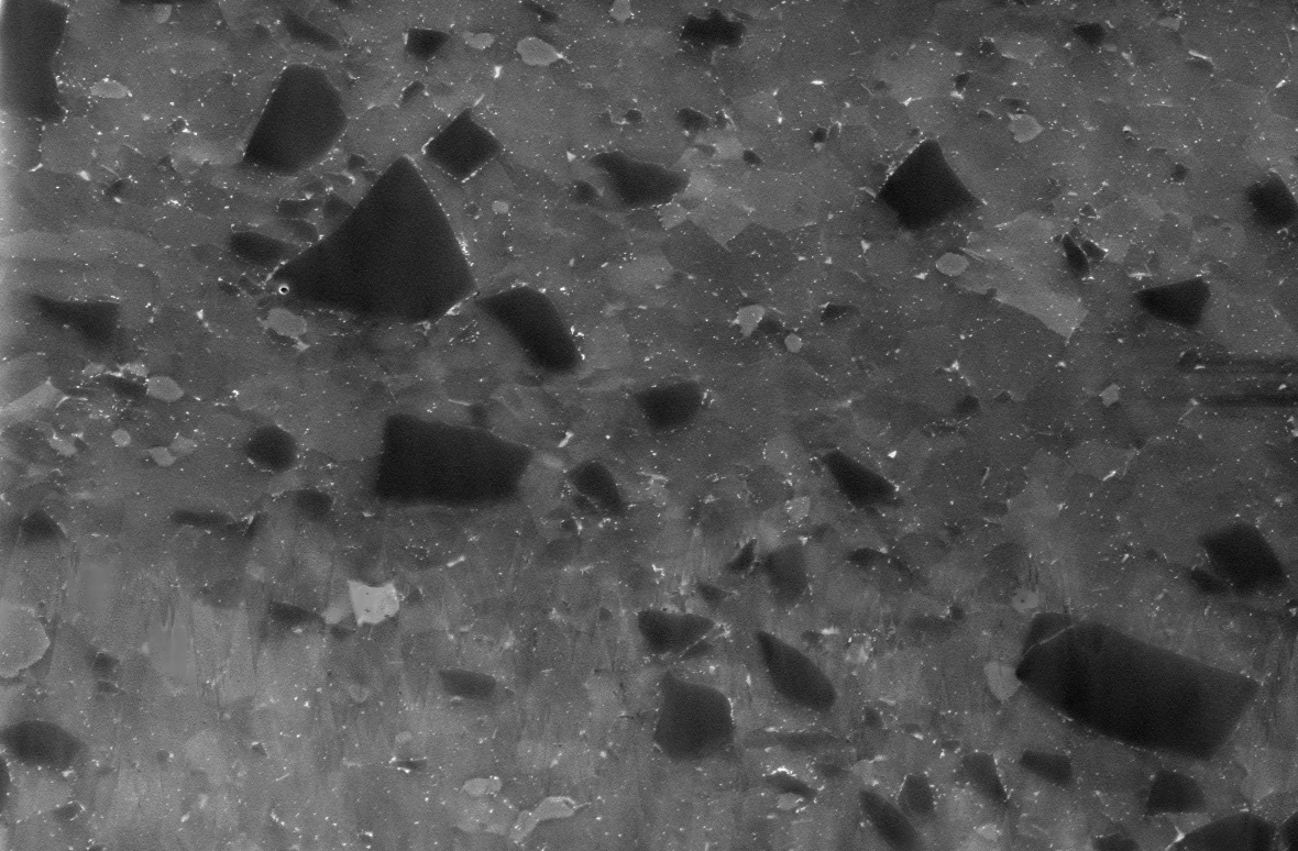
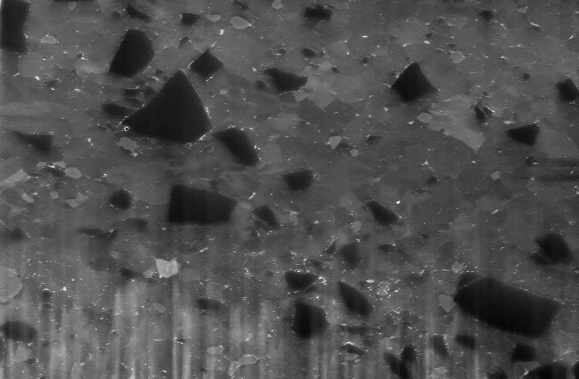
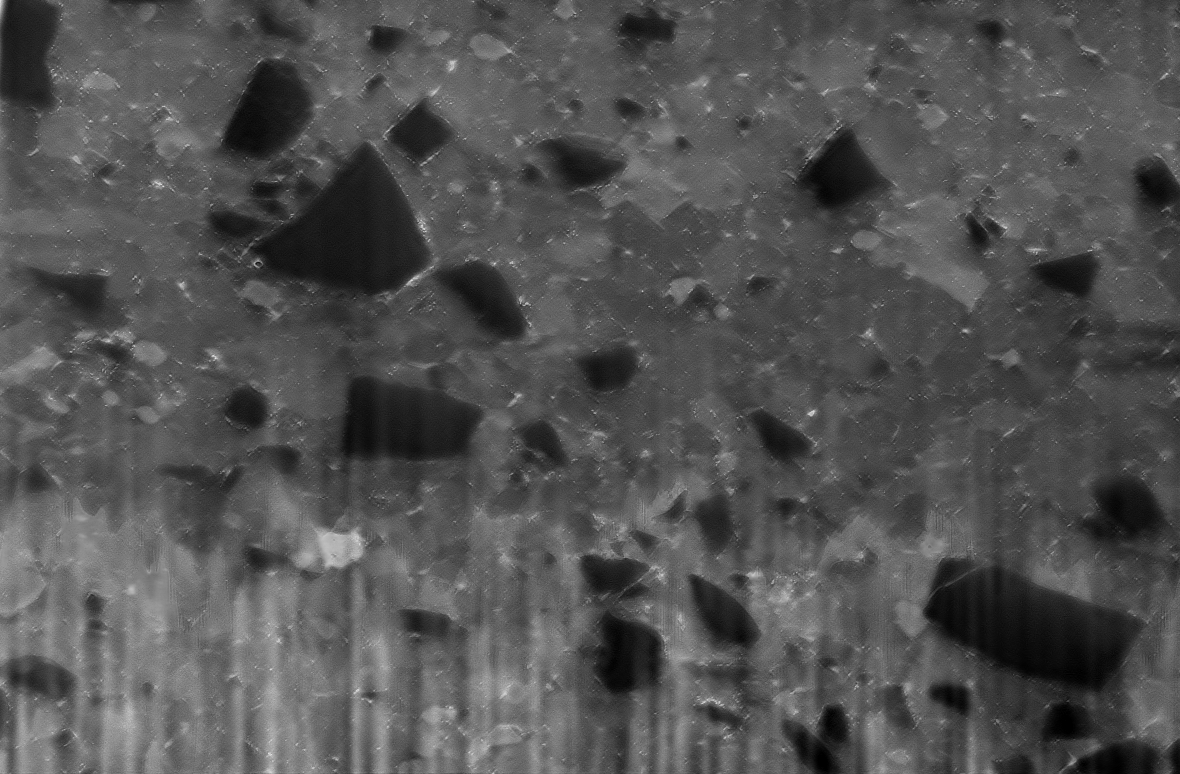
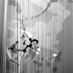
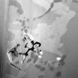
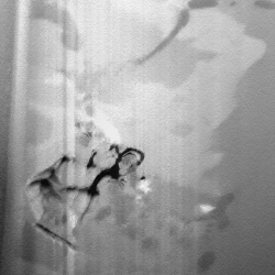
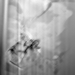
Unfortunately, such images often suffer from the so-called curtaining effect [19, 20, 43], see Fig. 2. This effect arises because the sputtering rates of the ion beam are sensitive to local changes in the surface structure. In particular below pores or cracks the rates vary and lead to stripe-like artifacts in the images. For the aluminum matrix composite in Fig. 2, e.g., at the phase boundary between aluminum and the reinforced silicon carbide particles, due to their locally varying material characteristics. Further, it may happen that the material is milled incompletely. This leads to bright laminar artifacts. To reduce the curtaining effects, a lower beam current could be used but this leads to a considerably higher milling time. Note that the whole imaging and milling process already takes about hours for each data set considered here. So further reducing the beam current leads to impractical processing times.
Therefore, we propose a computational model to reduce curtaining effects. The corruptions in our data consist both of stripe-like structures due to different sputtering rates and laminar structures due to incomplete milling of the material. The corrupted parts cannot be used for the further analysis of the material unless the curtaining effects are removed. For our specimen in Fig. 2 this was the case for more than half of the data. In FIB tomographic images the laminar corruptions are often cut off as they only occur in the lower part of the image. However, we will keep them since it is not desirable to throw away half of the data.
The problem of removing stripes in images was tackled by various approaches: Fourier based filtering was suggested in [13, 14], moment matching in [18] and histogram based methods in [24, 35]. Recently, variational models were successfully applied for the destriping of 2D images. The central idea in [5] is the application of unidirectional discrete TV terms to extract the stripes by minimizing the functional
| (1) |
where is the original image and the destriped one. This method was improved in [12] by adding a least squares data term and a framelet regularization term:
| (2) |
where denotes a Parseval framelet transform. It has been shown that this model gives much better results than the previous one also without framelet regularization, i.e. . The framelet regularization led to another slight improvement. Finally, a more general method for the variational denoising of images with structured noise was developed in [17], which has also been applied for destriping.
Applications of the aforementioned destriping methods are, e.g., the restoration of MODIS data [5, 12, 35] and FIB tomography images [12, 17]. In this paper, we focus mainly on the latter, where our FIB images are not only corrupted by stripe structured noise, but also by laminar effects. To the best of our knowledge the removal of curtaining effects involving additional large laminar parts was not considered before.
Compared to the above destriping methods our new model takes the following aspects into account:
-
A1)
The existing destriping methods remove stripes only. Since our data is not only corrupted by stripes, we split the corrupted image not only into a clean part and stripes, but also into a third, laminar part.
-
A2)
To avoid smoothing and to keep also the small image details, we use a hard constraint for the decomposition of the corrupted image into the clean, the striped and the laminar part by applying an infimal convolution model.
-
A3)
We consider 3D data whereas most destriping methods, except [17], focus on 2D images.
To deal with A2) we propose an infimal convolution model for the splitting. The infimal convolution was applied for the first time in image processing by Chambolle and Lions [9] followed by many other papers, see, e.g., the general discrete approach in [37] or the continuous function space approach in [23]. We also refer to a nice PhD thesis on infimal convolutions [40]. Infimal convolution models were in particular used for the decomposition of images.
Various variational decomposition models were proposed in the literature.
The additive splitting into geometric and oscillating parts as texture and white Gaussian noise
typically exploits TV- or Besov-seminorms for the first one
and
Meyers’s -norm [1, 28, 39],
the norm of the dual Sobolev space [30, 42], and
the squared -norm of the DCT-transformed texture [38]
for the second one. For specifying the noise component also the
norm of the dual Besov space was successfully used in [2].
Decomposition models were also applied for simultaneous structure-texture inpainting, e.g., in [3]
as an extension of the so-called morphological component analysis model [38].
For the separation of point and curved structures based on wavelets (Besov norms) and shearlets or curvelets we refer to [26, 38].
The clou of all these methods is the adaptation of the additive components to the task at hand.
For the curtaining problem we will show that our directional TV model is very well suited.
Organization of the Paper. In Section 2, we introduce our variational model for the removal of curtaining effects and motivate its choice by the special structure of the corruptions. Then, in Section 3, a primal dual algorithm is presented for finding a minimizer that consists of the clean image and two types of corruptions. Section 4 demonstrates the performance of our algorithm for volume images obtained by FIB tomography as well as artificial examples. Further, a comparison to existing methods for destriping and denoising of MODIS data is given. Finally, conclusions are drawn in Section 5.
2 New Model
We are given a 3D image corrupted by curtaining effects. The total corruption can be seen as an overlay of two parts:
-
i)
Laminar part consisting of very bright areas in the --plane. Along the -axis these regions occur very fluctuant and it is very unlikely that the effect appears in the same region in two subsequent frames.
-
ii)
Stripes along the -axis which are few pixels wide in and direction.
Based on the previous observations the corrupted image is assumed to be an additive composition of the clean image , the stripes and the laminar part of the corruptions , i.e., .
To give a sound discrete formulation of our model which takes i) and ii) into account, all images are considered as column- and slice-wise reshaped vectors in with . The reshaped images are denoted by small letters so that in particular . Then all linear operators can be written as matrices and their adjoints are just the transposed matrices. By we denote the Kronecker product of matrices. We use the following directional forward difference operators:
| (3) | |||
| (4) |
where
| (5) | ||||
| (6) |
and
| (7) | ||||
| (8) |
Note that we assume constant extension of the image beyond the boundary for the first order differences and linear extension for the second order differences which is exactly described by the matrix form of the operators. Let us further emphasize that we use the Kronecker product notation only for a correct description of our model in a convenient matrix-vector form. In our numerical computations we work with arrays based on the relation
| (9) |
for , , .
For a vector appearing, e.g., with after application of or and after applying , the grouped norm is given by
| (10) |
Finally, let denote the indicator function of a set defined by
We propose the following infimal convolution model
| (11) |
with
| (12) | ||||
| (13) | ||||
| (14) |
and regularization parameters . For convenience, we also add the definition of the above norms for the corresponding array formulation:
| (15) | ||||
| (16) | ||||
| (17) |
with the appropriate mirrored or linear extensions at the boundary. The last summand in ensures that the clean image has its range in . The choice of the other terms is motivated by i) and ii) as follows:
-
i)
and : laminar distortions have a small width in direction, thus a high response in the second order derivative is expected along this direction. Therefore, we penalize second order differences in direction of . Additionally, these corruptions are spacious in and direction such that a bidirectional TV regularizer is useful for .
-
ii)
and : stripes occur only in direction so that we penalize first order differences in direction of . This was also done in [5, 12] setting . Further, we penalize coupled first order differences in and direction of since we assume that the main differences along these directions occur in while has only few edges.
Remark 1.
Alternatively to we can also use the 3D TV term , i.e., instead of (11) we are asking for
| (18) |
where , are defined as in (11) and
| (19) |
The term for corresponds to the assumption that is a piecewise smooth image. Our model (11) focuses more on the corruptions. We argue in i) that, in contrast to the laminar corruptions, has a small second order derivative in direction. This viewpoint is also taken in [5, 12]. We have implemented both methods. The difference between the models is best visible in Fig. 4 in the numerical section.
Proposition 1 shows that our models (11) and (18) have a solution. Its uniqueness cannot be expected since arbitrary constants can be added to and subtracted from without changing the objective function.
The proof is given in the appendix.
3 Algorithm
In this section, we propose to use a primal dual algorithm to solve the convex, but non-smooth problem (11). Problem (18) can be handled in a similar way. Primal dual algorithms have recently found wide applications in image processing and machine learning. The reason is that these algorithms split the original task into a sequence of simple computable, proximal mappings. This paper cannot address the huge amount of papers on various primal dual strategies, which were successfully applied in imaging. For a good overview on primal dual methods we refer to [15, 25].
Recall that the proximal mapping of a proper, convex, lower semi continuous function is defined by
| (20) |
Indeed the proximal mapping at exists and is unique. To make primal dual algorithms efficient, the proximal mapping should in addition be simply computable. For applications of proximal mappings see, e.g., [31].
We want to apply the primal dual algorithm with an extrapolation of the dual variable suggested by Chambolle, Pock and Cremers in [10, 33], see also [11, 21, 32] for extensions. We call this algorithm PDHG (Primal Dual Hybrid Gradient) algorithm in accordance with the name of a similar algorithm which was presented without the extrapolation idea and without convergence proof in [44]. Later its convergence was examined in [4].
To this end, we have to rewrite our model (11). Using the vectors and and the notation
| (21) | ||||
| (22) |
we ask for
| (23) |
where
| (24) |
Then the PDHG algorithm from [10, 33] with an extrapolation of the dual variable reads
| (25) | ||||
| (26) | ||||
| (27) |
where denotes the conjugate function of and is the orthogonal projection onto . The algorithm converges if the parameters fulfill . For our structured matrix it is not hard to check by diagonalizing it with trigonometric transforms that , so that must be fulfilled.
Applying Moreau’s identity, one can directly work with the function instead of its conjugate. Using the rescaling , the algorithm becomes
| (28) | ||||
| (29) | ||||
| (30) | ||||
| (31) |
For details, see, e.g., [8]. Fortunately, the proximal mapping of can be separated into the proximal mappings of its summands with respect to , . The whole algorithm with our parameter choice is detailed in Algorithm 1.
| (32) | ||||
| (33) | ||||
| (34) | ||||
| (35) | ||||
| (36) | ||||
| (37) | ||||
| (38) | ||||
| (39) | ||||
| (40) | ||||
| (41) | ||||
| (42) |
The first step of the algorithm is a voxelwise projection onto the set . Since is just a plane with an additional range constraint for , this projection can be computed in a straightforward way. The update steps for and require a componentwise soft shrinkage, which is defined for by
| (43) |
For and a componentwise coupled shrinkage procedure is required. For vectors it is given by
| (44) |
Due to the separation of the computation of the , , the algorithm can be implemented in parallel on a multi-core architecture. Recently such parallel strategies were also examined by Pesquet and co-authors [7, 34]. Further we want to mention the interesting stochastic block coordinate algorithms in [16, 36].
4 Numerical Examples
In this section, we present the results of our algorithm, which was implemented in MATLAB2015b, for 3D artificial data, 3D FIB tomography data and 2D MODIS data. For the 3D examples, videos of the whole volume images are provided at our website http://www.mathematik.uni-kl.de/imagepro/members/fitschen/curtaining0/.
We compare the results of our model (11) with three other methods M1, M2 and M3 and with the modified model (18) in Remark 1. Since there seems to be no work especially on curtaining effects, the proposed methods are compared to the following 3D destriping and denoising algorithms:
-
M1)
Firstly, we generalize the 2D destriping approach from [12] with regularization terms as in (2) without the framelet part to 3D data, which results in
(45) To remove the corruptions that are not stripes, a median filter in direction is applied beforehand since the simple destriping algorithm is not able to remove these artifacts.
-
M2)
Secondly, we consider the 2D denoising method proposed in [17] for removing structured noise. We have used the implementation available at http://www.math.univ-toulouse.fr/~weiss/PageCodes.html
with a Gabor filter and parameters . Notice that this method is applicable for a wide range of structured noise. Thus one can not expect that the results are as good those of our model which is adjusted to this specific task. Again, we apply a median filter in direction first and then apply the algorithm to the 2D slices separately. -
M3)
Thirdly, we consider the 3D shearlet hard thresholding method in [27] for denoising of videos, see also [22]. We have used the software package ”ShearLab 3D” available at http://www.shearlab.org/software. For this method we have used the shearlet system , i.e., scales and a redundancy of . In total we have used different thresholding factors, one factor for the direction orthogonal to the laminar part, another one for the directions nearest to that direction, in the same way another two for the stripes () and finally a fifth factor for all other directions.
Compared to the methods M1 and M2 our method has the advantage of computing everything in one step without any preprocessing.
Artificial Data
The first two experiments deal with artificial 3D images disturbed by stripes and laminar structures, that are fluctuant in direction. The parameters of all models were chosen by an extensive grid search such that the PSNRs were optimized.
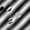
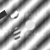
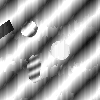
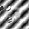
In Fig. 3, a comparison of the proposed models (11) and (18) and the methods M1, M2 and M3 is shown. Specific slices of the volume image are presented. The method (11) performs clearly better than the other ones. This is also confirmed by the corresponding PSNR values for the whole 3D data. If we apply M1 and M2 without a median filter in the preprocessing step, the PSNR is even worse, namely PSNR = 12.53 for the destriping method and PSNR = 10.05 for the denoising method. In contrast to these methods with M3 it is possible to remove the laminar part without an additional median filter. But nevertheless the results are clearly worse compared to the proposed model.
| corrupted | proposed (11) | proposed (18) |
 |
 |
 |
| M1 | M2 | M3 |
 |
 |
 |
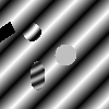
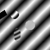
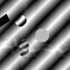
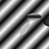
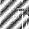
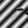
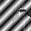
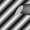
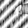
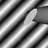
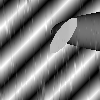
Comparing the models (11) and (18), we observe that the main differences occur along the laminar corruptions. To exclude that the reason for this behavior are the sharp edges of the laminar part, we show another example with a smoothed laminar part in Fig. 4. Model (11) gives an almost perfect reconstruction, whereas the method (18) is still not able to remove the laminar corruptions correctly. The results are summed up in Table 1.
| Image | Error measure | Model (11) | Model (18) | M1 | M2 | M3 |
|---|---|---|---|---|---|---|
| PSNR | ||||||
| Fig. 3 | MSE | |||||
| SSIM | ||||||
| PSNR | ||||||
| Fig. 4 | MSE | |||||
| SSIM |
Besides the PSNR, which we have discussed, the mean square error (MSE) and structural similarity index (SSIM) are stated in the table. In all cases our method (11) performs best and the methods M1, M2 and M3 are clearly worse.
| clean | corrupted | proposed (11) | proposed (18) |
|---|---|---|---|
 |
 |
 |
 |
 |
 |
 |
 |
 |
 |
 |
 |
FIB Data
Next we apply the methods to different FIB tomography data, namely to aluminum matrix composites with different particle sizes and to a bronze sample. The images of the aluminum matrix composite were obtained from the “Nano Structuring Center” Kaiserslautern and the bronze sample from the “Material Engineering Center Saarland” in Saarbrücken.
For all data sets we applied the proposed model (11) with the same parameters, namely
| (46) |
Only for the bronze sample we set since there is no laminar part.
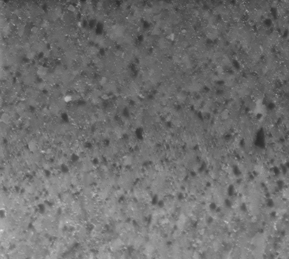
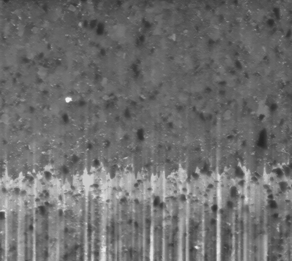
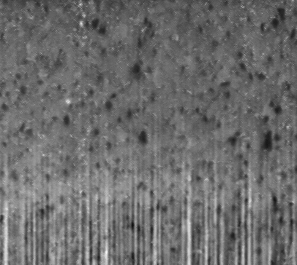
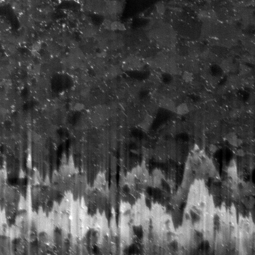
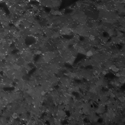
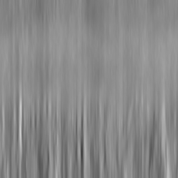
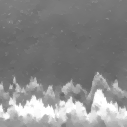
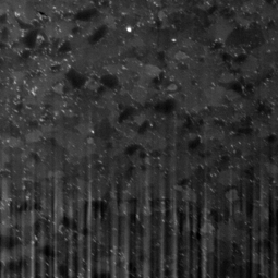
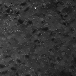
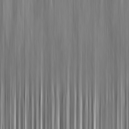
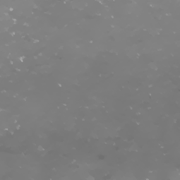
Fig. 5 demonstrates that our method (11) is able to split the corrupted image nicely into a clean image and two corrupted parts.
| corrupted | reconstructed | stripes | laminar |
|---|---|---|---|
 |
 |
 |
 |
 |
 |
 |
 |
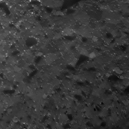
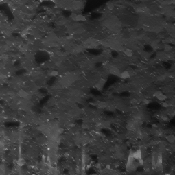
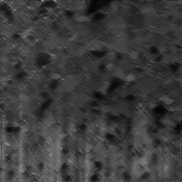
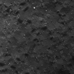
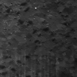
In Fig. 6, a comparison of our model (11) with (18), M1 and M3 is presented. For the slice that is mainly corrupted by stripes, M1 shows acceptable results, but cannot compete with (11) and (18), which perform equally well here. If there are not only stripes, one has to apply a median filter beforehand to obtain reasonable results with M1. However, this results in a loss of small image structures like the bright aggradations in the upper left part of the images. The method M3 leads to slightly smoothed results and still shows some remains of both stripes and the laminar part.
| original | proposed (11) | proposed (18) | M1 | M3 |
|---|---|---|---|---|
 |
 |
 |
 |
 |
 |
 |
 |
 |
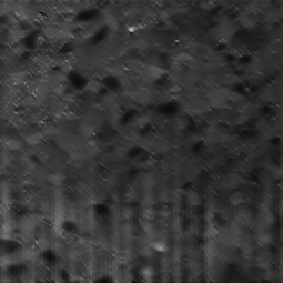 |
Finally, we show results obtained by our model (11) for FIB images of various materials. In Fig. 7 exemplary slices are shown. We obtain very good results although the materials as well as the corruptions look different. For a comparison also the results of M1 and M3 are presented. However, these are clearly worse. In particular with M1 the laminar structures are still present and M3 is not able to remove the stripes. But note that both methods are not designed for such corruptions.
MODIS Data
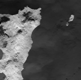
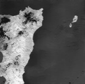
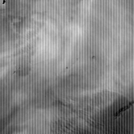
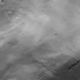
Our final experiments with 2D MODIS data (http://ladsweb.nascom.nasa.gov/index.html, also used in [5]) show that our method works also fine for destriping only. The parameters were chosen to give the best visual impression. The results of the various methods are presented in Fig. 8. For a comparison we have used the full model with the framelet regularization (2), proposed by [12], and the method M2. In both examples, all methods lead to visually good results. This shows that the proposed method can also be applied for destriping, although it is designed for the more general setting of stripes in combination with laminar corruptions.
5 Conclusions
We proposed a variational model for removing the curtaining effect in FIB tomography images. Due to the special structure of the corruptions, we chose an infimal convolution model consisting of directional TV terms and also second order terms for . Alternatively, a full 3D TV term for may be applied. The numerical experiments show that the proposed model leads to very good results. So far, all FIB tomography experiments share the same model parameters. This makes the method highly suitable for applications. Our restoration method enables us to use the FIB tomography results for the further (statistical) analysis of the 3D structure of the material, which was up to now only possible for a considerable smaller area of the data.
For future work we plan to parallelize the algorithm taking also spatial domain decompositions into account. The aim is an implementation of our approach in a way that it can be run simultaneously to the image acquisition process. Here we will also take other algorithms with potential on multicore architecture as e.g. [7, 34] into account.
Appendix A Appendix
Proof of Proposition 1: We rewrite (11) as
| (47) |
A feasible point is obviously given by and for some .
Assume that the infimum is not attained. Then there exists an infimal sequence , where so that
| (48) |
as . We will show that we can find another sequence with
| (49) |
Since this new sequence is bounded, there exists a converging subsequence. By the lower semi-continuity of this implies that the limit of this subsequence is a minimizer of contrary to the assumption.
It remains to show that there exists . Consider an arbitrary element of . Let the minimal and maximal value of the -th --plane of be denoted by , respectively . Then we have by and that . Now define
| (50) |
where .
Obviously, .
Further we have and by the constraint
on also .
Since the given image is also bounded, we conclude by
that is bounded, too. This finishes the proof.
Acknowledgement:
The authors thank
the anonymous referee for bringing model (18) to our attention,
P. Weiss (University of Toulouse) for providing the results for the MODIS data computed by the model M2 from [17],
K. Schladitz (Fraunhofer ITWM, Kaiserslautern), G. Steidl, F. Balle and T. Beck (University of Kaiserslautern) for fruitful discussions.
We are thankful to T. Löber (Nano Structuring Center Kaiserslautern) for creating FIB/SEM data of the aluminum matrix composite. We are grateful to the German Copper Institute (Deutsches Kupferinstitut Berufsverband e.V., DKI, Düsseldorf, Germany) for providing bronze samples and M. Engstler (Material Engineering Center Saarland (MECS), Steinbeis Research Center, Saarbrücken, Germany) for providing FIB/SEM data of bronze samples.
Funding by the German Research Foundation (DFG) within the Research Training Group 1932 ”Stochastic Models for Innovations in the Engineering Sciences”, project area P3, is gratefully acknowledged.
References
- [1] J.-F. Aujol, G. Aubert, L. Blanc-Féraud, and A. Chambolle. Image decomposition application to SAR images. In Scale Space Methods in Computer Vision, pages 297–312. Springer, 2003.
- [2] J.-F. Aujol and A. Chambolle. Dual norms and image decomposition models. International Journal of Computer Vision, 63(1):85–104, 2005.
- [3] J.-F. Aujol, G. Gilboa, T. Chan, and S. Osher. Structure-texture image decomposition—modeling, algorithms, and parameter selection. International Journal of Computer Vision, 67(1):111–136, 2006.
- [4] S. Bonettini and V. Ruggiero. On the convergence of primal-dual hybrid gradient algorithms for total variation image restoration. Journal of Mathematical Imaging and Vision, 44(3):236–253, 2012.
- [5] M. Bouali and S. Ladjal. Toward optimal destriping of MODIS data using a unidirectional variational model. IEEE Transactions on Geoscience and Remote Sensing, 49(8):2924–2935, 2011.
- [6] D. Brandon and W. D. Kaplan. Microstructural Characterization of Materials. John Wiley and Sons, Ltd, 2008.
- [7] L. Briceño-Arias, P. Combettes, J.-C. Pesquet, and N. Pustelnik. Proximal algorithms for multicomponent image recovery problems. Journal of Mathematical Imaging and Vision, 41(1-2):3–22, 2011.
- [8] M. Burger, A. Sawatzky, and G. Steidl. First order algorithms in variational image processing. In S. O. R. Glowinski and W. Yin, editors, To appear in Operator Splittings and Alternating Direction Methods, 2014.
- [9] A. Chambolle and P.-L. Lions. Image recovery via total variation minimization and related problems. Numerische Mathematik, 76(2):167–188, 1997.
- [10] A. Chambolle and T. Pock. A first-order primal-dual algorithm for convex problems with applications to imaging. Journal of Mathematical Imaging and Vision, 40(1):120–145, 2011.
- [11] A. Chambolle and T. Pock. On the ergodic convergence rates of a first-order primal-dual algorithm. To appear in Math. Programm. A, 2015.
- [12] Y. Chang, H. Fang, L. Yan, and H. Liu. Robust destriping method with unidirectional total variation and framelet regularization. Optics Express, 21(20):23307–23323, 2013.
- [13] J. Chen, Y. Shao, H. Guo, W. Wang, and B. Zhu. Destriping CMODIS data by power filtering. IEEE Transactions on Geoscience and Remote Sensing, 41(9):2119–2124, 2003.
- [14] S.-w. Chen and J.-L. Pellequer. DeStripe: frequency-based algorithm for removing stripe noises from AFM images. BMC Structural Biology, 11(1):7, 2011.
- [15] P. L. Combettes and J.-C. Pesquet. Proximal splitting methods in signal processing. In H. H. Bauschke, R. S. Burachik, P. L. Combettes, V. Elser, D. R. Luke, and H. Wolkowicz, editors, Fixed-Point Algorithms for Inverse Problems in Science and Engineering, volume 49 of Springer Optimization and Its Applications, pages 185–212. Springer New York, 2011.
- [16] P. L. Combettes and J.-C. Pesquet. Stochastic quasi-Fejér block-coordinate fixed point iterations with random sweeping. SIAM Journal on Optimization, 25(2):1221–1248, 2015.
- [17] J. Fehrenbach, P. Weiss, and C. Lorenzo. Variational algorithms to remove stationary noise: Applications to microscopy imaging. IEEE Transactions on Image Processing, 21(10):4420–4430, 2012.
- [18] F. L. Gadallah, F. Csillag, and E. J. M. Smith. Destriping multisensor imagery with moment matching. International Journal of Remote Sensing, 21(12):2505–2511, 2000.
- [19] L. A. Giannuzzi and F. A. Stevie. A review of focused ion beam milling techniques for TEM specimen preparation. Micron, 30(3):197–204, 1999.
- [20] L. A. Giannuzzi and F. A. Stevie. Introduction to Focused Ion Beams: Instrumentation, Theory, Techniques and Practice. Springer US, 2005.
- [21] T. Goldstein, E. Esser, and R. Baraniuk. Adaptive primal-dual hybrid gradient methods for saddle-point problems. ArXiv Preprint 1305.0546, 2013.
- [22] B. Heise, S. E. Schausberger, S. Häuser, B. Plank, D. Salaberger, E. Leiss-Holzinger, and D. Stifter. Full-field optical coherence microscopy with a sub-nanosecond supercontinuum light source for material research. Optical Fiber Technology, 18(5):403–410, 2012.
- [23] M. Holler and K. Kunisch. On infimal convolution of TV-type functionals and applications to video and image reconstruction. SIAM Journal on Imaging Sciences, 7(4):2258–2300, 2014.
- [24] B. K. Horn and R. J. Woodham. Destriping LANDSAT MSS images by histogram modification. Computer Graphics and Image Processing, 10(1):69 – 83, 1979.
- [25] N. Komodakis and J. C. Pesquet. Playing with duality: An overview of recent primal-dual approaches for solving large-scale optimization problems. IEEE Signal Processing Magazine, 32(6):31–54, 2015.
- [26] G. Kutyniok and W.-Q. Lim. Image separation using wavelets and shearlets. In Curves and Surfaces, pages 416–430. Springer, Berlin-Heidelberg, 2012.
- [27] G. Kutyniok, W.-Q. Lim, and R. Reisenhofer. ShearLab 3D: Faithful digital shearlet transforms based on compactly supported shearlets. ArXiv Preprint 1402.5670, 2014.
- [28] Y. Meyer. Oscillating patterns in image processing and nonlinear evolution equations. American Mathematical Society, Boston, USA, 2001.
- [29] P. Munroe. The application of focused ion beam microscopy in the material sciences. Materials Characterization, 60(1):2 – 13, 2009.
- [30] S. Osher, A. Solé, and L. Vese. Image decomposition and restoration using total variation minimization and the . Multiscale Modeling & Simulation, 1(3):349–370, 2003.
- [31] N. Parikh and S. Boyd. Proximity algorithms. Foundations and Trends in Optimization, 1(3):123–231, 2013.
- [32] T. Pock and A. Chambolle. Diagonal preconditioning for first order primal-dual algorithms in convex optimization. In IEEE International Conference on Computer Vision, pages 1762–1769, 2011.
- [33] T. Pock, A. Chambolle, D. Cremers, and H. Bischof. A convex relaxation approach for computing minimal partitions. In IEEE Conference on Computer Vision and Pattern Recognition, pages 810–817. 2009.
- [34] N. Pustelnik, C. Chaux, and J. Pesquet. Parallel proximal algorithm for image restoration using hybrid regularization. IEEE Transactions on Image Processing, 20(9):2450–2462, 2011.
- [35] P. Rakwatin, W. Takeuchi, and Y. Yasuoka. Stripe noise reduction in MODIS data by combining histogram matching with facet filter. IEEE Transactions on Geoscience and Remote Sensing, 45(6):1844–1856, 2007.
- [36] A. Repetti, E. Chouzenoux, and J.-C. Pesquet. A random block-coordinate primal-dual proximal algorithm with application to 3D mesh denoising. In Proceedings of the IEEE International Conference on Acoustics, Speech, and Signal Processing, 2015.
- [37] S. Setzer, G. Steidl, and T. Teuber. Infimal convolution regularizations with discrete -type functionals. Communications in Mathematical Sciences, 9(3):797–872, 2011.
- [38] J.-L. Starck, F. Murtagh, and J. M. Fadili. Sparse Image and Signal Processing: Wavelets, Curvelets, Morphological Diversity. Cambridge University Press, New York, USA, 2010.
- [39] D. M. Strong, J.-F. Aujol, and T. F. Chan. Scale recognition, regularization parameter selection, and Meyer’s G norm in total variation regularization. Multiscale Modeling & Simulation, 5(1):273–303, 2006.
- [40] T. Strömberg. The operation of infimal convolution. Dissertationes Mathematicae (Rozprawy Matematyczne). 1996.
- [41] A. Velichko, C. Holzapfel, A. Siefers, K. Schladitz, and F. Mücklich. Unambiguous classification of complex microstructures by their three-dimensional parameters applied to graphite in cast iron. Acta Materialia, 56(9):1981 – 1990, 2008.
- [42] L. A. Vese and S. J. Osher. Modeling textures with total variation minimization and oscillating patterns in image processing. Journal of Scientific Computing, 19(1-3):553–572, 2003.
- [43] S. Zaefferer, S. Wright, and D. Raabe. Three-dimensional orientation microscopy in a focused ion beam–scanning electron microscope: A new dimension of microstructure characterization. Metallurgical and Materials Transactions A, 39(2):374–389, 2008.
- [44] M. Zhu and T. Chan. An efficient primal-dual hybrid gradient algorithm for total variation image restoration. Technical report, UCLA, Center for Applied Math., 2008.
