Models for extremal dependence derived from skew-symmetric families

Abstract

Skew-symmetric families of distributions such as the skew-normal and skew-$t$ represent supersets of the normal and $t$ distributions, and they exhibit richer classes of extremal behaviour. By defining a non-stationary skew-normal process, which allows the easy handling of positive definite, non-stationary covariance functions, we derive a new family of max-stable processes – the extremal-skew-$t$ process. This process is a superset of non-stationary processes that include the stationary extremal-$t$ processes. We provide the spectral representation and the resulting angular densities of the extremal-skew-$t$ process, and illustrate its practical implementation

Keywords: Asymptotic independence; Angular density; Extremal coefficient; Extreme values; Max-stable distribution; Non-central extended skew-t distribution; Non-stationarity; Skew-Normal distribution; Skew-Normal process; Skew-$t$ distribution.

1 Introduction

The modern-day analysis of extremes is based on results from the theory of stochastic processes. In particular, max-stable processes (de Haan, 1984) are a popular and useful tool when modelling extremal responses in environmental, financial and engineering applications. Let $\mathbb{S}\subseteq{\mathbb{R}}^{k}$ denote a $k$-dimensional region of space (or space-time) over which a real-valued stochastic process $\{Y(s)\}_{s\in\mathbb{S}}$ with a continuous sample path on $\mathbb{S}$ can be defined. Considering a sequence $Y_{1},\ldots,Y_{n}$ of independent and identically distributed (iid) copies of $Y$, the pointwise partial maximum can be defined as

$$M_{n}(s)=\max_{i=1,\ldots,n}Y_{i}(s),\quad s\in\mathbb{S}.$$

If there are sequences of real-valued functions, $a_{n}(s)>0$ and $b_{n}(s)$, for $s\in\mathbb{S}$ and $n=1,2,\ldots$, such that

$$\left\{\frac{M_{n}(s)-b_{n}(s)}{a_{n}(s)}\right\}_{s\in\mathbb{S}}\Rightarrow\{U(s)\}_{s\in\mathbb{S}},$$

converges weakly as $n\rightarrow\infty$ to a process $U(s)$ with non-degenerate marginal distributions for all $s\in\mathbb{S}$, then $U(s)$ is known as a max-stable process (de Haan and Ferreira, 2006, Ch. 9). In this setting, for a finite sequence of points $(s_{j})_{j\in I}$ in $\mathbb{S}$, where $I=\{1,\ldots,d\}$ is an index set, the finite-dimensional distribution of $U$ is then a multivariate extreme value distribution (de Haan and Ferreira, 2006, Ch. 6). This distribution has generalised extreme value univariate margins and, when parameterised with unit Fréchet margins, has a joint distribution function of the form

$$G(x_{j},j\in I)=\exp\{-V(x_{j},j\in I)\},\quad x_{j}>0,$$

where $x_{j}\equiv x(s_{j})$. The exponent function $V$ describes the dependence between extremes, and can be expressed as

$$V(x_{j},j\in I)=\int_{\mathbb{W}}\max_{j\in I}(w_{j}/x_{j})H(\text{d}w_{1},\ldots,\text{d}w_{d}),$$

where the angular measure $H$ is a finite measure defined on the $d$-dimensional unit simplex $\mathbb{W}=\{w\in{\mathbb{R}}^{d}:w_{1}+\cdots+w_{d}=1\},$ satisfying the moment conditions $\int_{\mathbb{W}}w_{j}\;H(\text{d}w)=1,j\in I,$ (de Haan and Ferreira, 2006, Ch. 6).

In recent years a variety of specific max-stable processes have been developed, many of which have become popular as they can be practically amenable to statistical modelling (Davison et al., 2012). The extremal-$t$ process (Opitz, 2013) is one of the best-known and widely-used max-stable processes, from which the Brown-Resnick process (Brown and Resnick, 1977, Kabluchko et al., 2009), the Gaussian extreme-value process (Smith, 1990) and the extremal-Gaussian processes (Schlather, 2002) can be seen as special cases. In their most basic form, the Brown-Resnick and the extremal-$t$ processes can be respectively understood as the limiting extremal processes of strictly stationary Gaussian and Student-$t$ processes. However, in practice, data may be non-stationary and exhibit asymmetric distributions in many applications. In these scenarios, skew-symmetric distributions (Azzalini, 2013, Arellano-Valle and Azzalini, 2006, Azzalini, 2005, Genton, 2004, Azzalini, 1985) provide simple models for modelling asymmetrically distributed data. However, the limiting extremal behaviour of these processes has not yet been established.

In this paper we characterise and develop statistical models for the extremal behaviour of skew-normal and skew-$t$ distributions. The joint tail behaviours of these skew distributions are capable of describing a far wider range of dependence levels than that obtained under the symmetric normal and $t$ distributions. We provide a definition of a skew-normal process which is in turn a non-stationary process. This provides an accessible approach to constructing positive definite, non-stationary covariance functions when working with non-Gaussian processes. Recently some forms of non-stationary dependent structures embedded into max-stable processes have been studied by Huser and Genton (2015). We show that on the basis of the skew-normal process a new family of max-stable processes – the extremal-skew-$t$ process – can be obtained. This process is a superset of non-stationary processes that includes the stationary extremal-$t$ processes (Opitz, 2013). From the extremal-skew-$t$ process, a rich family of non-stationary, isotropic or anisotropic extremal coefficient functions can be obtained.

This paper is organised as follows: in Section 2 we first introduce a new variant of the extended skew-$t$ class of distributions, before developing a non-stationary version of the skew-normal process. In both cases we discuss the stochastic behavior of their extreme values. In Section 3 we derive the spectral representation of the extended extremal skew-$t$ process. Section 4 discusses inferential aspects of the extremal skew-$t$ dependence model, and Section 5 provides a real data application. We conclude with a Discussion.

2 Preliminary results on skew-normal processes and skew-$t$ distributions

We introduce two preliminary results that will be used in order to present our main contribution in Section 3, the extremal-skew-$t$ process. In Section 2.1 we define the non-central extended skew-$t$ family of distributions, which is a new variant of the class introduced by Arellano-Valle and Genton (2010), that allows a non-centrality parameter. In Section 2.2 we present the development of a new non-stationary, skew normal random process.

Hereafter, we use $Y\sim\mathcal{D}_{d}(\theta_{1},\theta_{2},\ldots)$ to denote that $Y$ is a $d$-dimensional random vector with probability law $\mathcal{D}$ and parameters $\theta_{1},\theta_{2},\ldots$. When $d=1$ the subscript is omitted for brevity. Similarly, when a parameter is equal to zero or a scale matrix is equal to the identity (both in a vector and scalar sense) so that $\mathcal{D}_{d}$ reduces to an obvious sub-family, it is also omitted.

2.1 The non-central, extended skew-$t$ distribution

While several skew-symmetric distributions have been developed (see e.g., Genton, 2004, Azzalini, 2013), we focus on the skew-normal and skew-$t$ distributions.

Denote a $d$-dimensional skew-normally distributed random vector by $Y\sim\mathcal{S}\mathcal{N}_{d}(\mu,\Omega,\alpha,\tau)$ (Arellano-Valle and Genton, 2010). This random vector has probability density function (pdf)

$$\phi_{d}(y;\mu,\Omega,\alpha,\tau)=\frac{\phi_{d}(y;\mu,\Omega)}{\Phi\{\tau/\sqrt{1+Q_{\bar{\Omega}}(\alpha)}\}}\,\Phi(\alpha^{\top}z+\tau),\qquad y\in{\mathbb{R}}^{d},$$ (1)

where $\phi_{d}(y;\mu,\Omega)$ is a $d$-dimensional normal pdf with mean $\mu\in{\mathbb{R}}^{d}$ and $d\times d$ covariance matrix $\Omega$, $z=(y-\mu)/\omega$, $\omega=\mbox{diag}(\Omega)^{1/2}$, $\bar{\Omega}=\omega^{-1}\,\Omega\,\omega^{-1}$, $Q_{\bar{\Omega}}(\alpha)=\alpha^{\top}\bar{\Omega}\alpha$ and $\Phi(\cdot)$ is the standard univariate normal cumulative distribution function (cdf). The shape parameters $\alpha\in{\mathbb{R}}^{d}$ and $\tau\in{\mathbb{R}}$ are respectively slant and extension parameters. The cdf associated with (1) is termed the extended skew-normal distribution (Arellano-Valle and Genton, 2010) of which the skew-normal and normal distributions are special cases (Arellano-Valle and Genton, 2010, Azzalini, 2013). For example, in the case where $\alpha=0$ and $\tau=0$ the standard normal pdf is recovered.

Definition 1.

$Y$ is a $d$-dimensional, non-central extended skew-$t$ distributed random vector, denoted by $Y\sim\mathcal{S}\mathcal{T}_{d}(\mu,\Omega,\alpha,\tau,\kappa,\nu)$, if for $y\in{\mathbb{R}}^{d}$ it has pdf

$$\psi_{d}(y;\mu,\Omega,\alpha,\tau,\kappa,\nu)=\frac{\psi_{d}(y;\mu,\Omega,\nu)}{\Psi\left(\frac{\tau}{\sqrt{1+Q_{\bar{\Omega}}(\alpha)}};\frac{\kappa}{\sqrt{1+Q_{\bar{\Omega}}(\alpha)}},\nu\right)}\Psi\left\{(\alpha^{\top}z+\tau)\sqrt{\frac{\nu+d}{\nu+Q_{\bar{\Omega}^{-1}}(z)}};\kappa,\nu+d\right\},$$ (2)

where $\psi_{d}(y;\mu,\Omega,\nu)$ is the pdf of a $d$-dimensional $t$-distribution with location $\mu\in{\mathbb{R}}^{d}$, $d\times d$ scale matrix $\Omega$ and $\nu\in\mathbb{R}^{+}$ degrees of freedom, $\Psi(\cdot;a,\nu)$ denotes a univariate non-central $t$ cdf with non-centrality parameter $a\in{\mathbb{R}}$ and $\nu$ degrees of freedom, and $Q_{\bar{\Omega}^{-1}}(z)=z^{\top}\bar{\Omega}^{-1}z$. The remaining terms are as defined in (1). The associated cdf is

$$\Psi_{d}(y;\mu,\Omega,\alpha,\tau,\kappa,\nu)=\frac{\Psi_{d+1}\left\{\bar{z};\Omega^{*},\kappa^{*},\nu\right\}}{\Psi\left(\bar{\tau};\bar{\kappa},\nu\right)},$$ (3)

where $\bar{z}=(z^{\top},\bar{\tau})^{\top}$, $\Psi_{d+1}$ is a $(d+1)$-dimensional (non-central) $t$ cdf with covariance matrix and non-centrality parameters

$$\Omega^{*}=\left(\begin{array}[]{cc}\bar{\Omega}&-\delta\\ -\delta^{\top}&1\end{array}\right),\quad\kappa^{*}=\left(\begin{array}[]{c}0\\ \bar{\kappa}\end{array}\right),$$

and $\nu$ degrees of freedom, and where

$$\delta=\left\{1+Q_{\bar{\Omega}}(\alpha)\right\}^{-1/2}\,\bar{\Omega}\alpha,\quad\bar{\kappa}=\left\{1+Q_{\bar{\Omega}}(\alpha)\right\}^{-1/2}\,\kappa,\quad\bar{\tau}=\left\{1+Q_{\bar{\Omega}}(\alpha)\right\}^{-1/2}\,\tau.$$ (4)

When the non-centrality parameter $\kappa$ is zero, then the extended skew-$t$ family of Arellano-Valle and Genton (2010) is obtained. For the non-central skew-$t$ family, we now demonstrate modified properties to those discussed in Arellano-Valle and Genton (2010).

Proposition 1 (Properties).

Let $Y\sim\mathcal{S}\mathcal{T}_{d}(\mu,\Omega,\alpha,\tau,\kappa,\nu)$.

1. Marginal and conditional distributions. Let $I\subset\{1,\ldots,d\}$ and $\bar{I}=\{1,\ldots,d\}\backslash I$ identify the $d_{I}$- and $d_{\bar{I}}$-dimensional subvector partition of $Y$ such that $Y=(Y_{I}^{\top},Y_{\bar{I}}^{\top})^{\top}$, with corresponding partitions of the parameters $(\mu,\Omega,\alpha)$. Then

   1. $Y_{I}\sim\mathcal{S}\mathcal{T}_{d_{I}}(\mu_{I},\Omega_{II},\alpha^{*}_{I},\tau^{*}_{I},\kappa^{*}_{I},\nu)$, where

      $$\begin{array}[]{ccc}\alpha^{*}_{I}=\frac{\alpha_{I}+\bar{\Omega}_{II}^{-1}\bar{\Omega}_{I\bar{I}}\alpha_{\bar{I}}}{\sqrt{1+Q_{\tilde{\Omega}_{\bar{I}\bar{I}\cdot I}}(\alpha_{\bar{I}})}},&\tau^{*}_{I}=\frac{\tau}{\sqrt{1+Q_{\tilde{\Omega}_{\bar{I}\bar{I}\cdot I}}(\alpha_{\bar{I}})}},&\kappa^{*}_{I}=\frac{\kappa}{\sqrt{1+Q_{\tilde{\Omega}_{\bar{I}\bar{I}\cdot I}}(\alpha_{\bar{I}})}},\end{array}$$ (6)

      given $\tilde{\Omega}_{\bar{I}\bar{I}\cdot I}=\bar{\Omega}_{\bar{I}\bar{I}}-\bar{\Omega}_{\bar{I}I}\bar{\Omega}_{II}^{-1}\bar{\Omega}_{I\bar{I}}.$

   2. $(Y_{\bar{I}}|Y_{I}=y_{I})\sim\mathcal{S}\mathcal{T}_{d_{\bar{I}}}(\mu_{\bar{I}\cdot I},\Omega_{\bar{I}\cdot I},\alpha_{\bar{I}\cdot I},\tau_{\bar{I}\cdot I},\kappa_{\bar{I}\cdot I},\nu_{\bar{I}\cdot I})$, where $\mu_{\bar{I}\cdot I}=\mu_{\bar{I}}+\Omega_{I\bar{I}}\Omega_{II}^{-1}(y_{I}-\mu_{I})$, $\Omega_{\bar{I}\cdot I}=\zeta_{I}\Omega_{\bar{I}\bar{I}\cdot I}$, $\zeta_{I}=\{\nu+Q_{\Omega_{II}^{-1}}(z_{I})\}/(\nu+d_{I})$, $z_{I}=\omega_{I}^{-1}(y_{I}-\mu_{I})$, $\omega_{I}=\mbox{diag}(\omega_{II})^{1/2}$, $Q_{\Omega_{II}^{-1}}(z_{I})=z_{I}^{\top}\Omega_{II}^{-1}z_{I}$, $\Omega_{\bar{I}\bar{I}\cdot I}=\Omega_{\bar{I}\bar{I}}-\Omega_{\bar{I}I}\Omega_{II}^{-1}\Omega_{I\bar{I}}$, $\alpha_{\bar{I}\cdot I}=\omega_{\bar{I}\cdot I}\omega_{\bar{I}}^{-1}\alpha_{\bar{I}}$, $\omega_{\bar{I}\cdot I}=\mbox{diag}(\Omega_{\bar{I}\bar{I}\cdot I})^{1/2}$, $\omega_{\bar{I}}=\mbox{diag}(\omega_{\bar{I}\bar{I}})^{1/2}$, $\tau_{\bar{I}\cdot I}=\zeta_{I}^{-1/2}\{(\alpha_{\bar{I}}^{\top}\bar{\Omega}_{\bar{I}I}\bar{\Omega}_{II}^{-1}+\alpha_{I}^{\top})z_{I}+\tau\}$, $\kappa_{\bar{I}\cdot I}=\zeta_{I}^{-1/2}\kappa$ and $\nu_{\bar{I}\cdot I}=\nu+d_{I}$.

2. Conditioning type stochastic representation. We can write $Y=\mu+\Omega Z$, where $Z=(X|\alpha^{\top}X+\tau>X_{0}),$ and where $X\sim\mathcal{T}_{d}(\bar{\Omega},\nu)$ is independent of $X_{0}\sim\mathcal{T}(\kappa,\nu)$.

3. Additive type stochastic representation. We can write $Y=\mu+\Omega Z$, where $Z=\sqrt{\frac{\nu+\tilde{X}_{0}^{2}}{\nu+1}}X_{1}+\delta\tilde{X}_{0},$ $X_{1}\sim\mathcal{T}_{d}(\Omega-\delta\delta^{\top},\bar{\kappa},\nu+1)$ is independent of $\tilde{X}_{0}=(X_{0}|X_{0}+\bar{\tau}>0)$, $X_{0}\sim\mathcal{T}(\bar{\kappa},\nu)$, $\delta\in(-1,1)^{d}$ and where $\bar{\tau}$ and $\bar{\kappa}$ are as in (4).

Proof in Appendix A.1

We conclude by presenting a final property of the non-central skew-$t$ family. The next result describes the extremal behaviour of observations drawn from a member of this class.

Proposition 2.

Let $Z_{1},\ldots,Z_{n}$ be iid copies of $Z\sim\mathcal{S}\mathcal{T}_{d}(\bar{\Omega},\alpha,\tau,\kappa,\nu)$ and $M_{n}$ be the componentwise sample maxima. Define $a_{n}=(a_{n,1},\ldots,a_{n,d})^{\top}$, where

$$a_{n,j}=\left\{\frac{n\{\Gamma(\nu/2)\}^{-1}\Gamma\{(\nu+1)/2\}\nu^{(\nu-2)/2}\,\Psi(\alpha^{*}_{j}\sqrt{\nu+1};\kappa,\nu+1)}{\sqrt{\pi}\Psi\left(\tau^{*}_{j}/\{1+Q_{\bar{\Omega}}(\alpha^{*}_{j})\}^{1/2};\kappa^{*}_{j}/\{1+Q_{\bar{\Omega}}(\alpha^{*}_{j})\},\nu\right)}\right\}^{1/\nu}$$

where $\alpha^{*}_{j}=\alpha^{*}_{\{j\}}$, $\tau^{*}_{j}=\tau^{*}_{\{j\}}$ and $\kappa^{*}_{j}=\kappa^{*}_{\{j\}}$ are the marginal parameters (6) under Proposition 1(1). Then $M_{n}/a_{n}\Rightarrow U$ as $n\rightarrow+\infty$, where $U$ has univariate $\nu$-Fréchet marginal distributions (i.e. $e^{-x^{-\nu}}$, $x>0$), and exponent function

$$V(x_{j},j\in I)=\sum_{j=1}^{d}x_{j}^{-\nu}\Psi_{d-1}\left(\left(\sqrt{\frac{\nu+1}{1-\omega^{2}_{i,j}}}\left(\frac{x^{+}_{i}}{x^{+}_{j}}-\omega_{i,j}\right),i\in I_{j}\right)^{\top};\bar{\Omega}^{+}_{j},\alpha^{+}_{j},\tau^{+}_{j},\nu+1\right),$$ (7)

where $\Psi_{d-1}$ is a $(d-1)$-dimensional central extended skew-$t$ distribution with correlation matrix $\bar{\Omega}^{+}_{j}$, shape and extension parameters $\alpha^{+}_{j}$ and $\tau^{+}_{j}$, and $\nu+1$ degrees of freedom, $I=\{1,\ldots,d\}$, $I_{j}=I\backslash\{j\}$, and $\omega_{i,j}$ is the $(i,j)$-th element of $\bar{\Omega}$.

Proof (and further details) in Appendix A.2.

As the limiting distribution (7) is the same as that of the classic skew-$t$ distribution (see Padoan, 2011), it exhibits identical upper and lower tail dependence coefficients (e.g. Joe, 1997, Ch 5). That is, the extension and non-centrality parameters, $\tau$ and $\kappa$, do not affect the extremal behavior.

2.2 A non-stationary, skew-normal random process

While there are several definitions of a stationary skew-normal process (e.g. Minozzo and Ferracuti, 2012), stationarity is incompatible with the requirement that all finite-dimensional distributions of the process are skew-normal. We now construct a non-stationary version of the skew-normal process through the additive-type stochastic representation (e.g. Azzalini, 2013, Ch. 5). A similar approach was explored by Zhang and El-Shaarawi (2010) for the stationary case.

Definition 2.

Let {$X(s)\}_{s\in\mathbb{S}}$ be a stationary Gaussian random process on $\mathbb{S}$ with zero mean, unit variance and correlation function $\rho(h)={\mathbb{E}}\{X(s)X(s+h)\}$ for $s\in\mathbb{S}$ and $h\in{\mathbb{R}}^{k}$. For $X^{\prime}\sim\mathcal{N}(0,1)$ independent of $X(s)$, $\varepsilon\in\mathbb{R}$ and a function $\delta:\mathbb{S}\mapsto(-1,1)$, define

$$X^{\prime\prime}(s) := X^{\prime}|X^{\prime}+\varepsilon>0,\qquad\forall\;s\in\mathbb{S}$$

$$Z(s) := \sqrt{1-\delta(s)^{2}}X(s)+\delta(s)X^{\prime\prime}(s),\quad s\in\mathbb{S}.$$ (8)

Then $Z(s)$ is a skew-normal random process.

We refer to $\delta(s)$ as the slant function. From (8), if $\delta(s)\equiv 0$ for all $s\in\mathbb{S}$, then $Z$ is a Gaussian random process. Note that $Z$ is a random process with a consistent family of distribution functions, since $Z(s)=a(s)X(s)+b(s)Y(s)$ where $a$ and $b$ are bounded functions and $X$ and $Y$ are random processes with a consistent family of distribution functions. For any finite sequence of points $s_{1},\ldots,s_{d}\in\mathbb{S}$ the joint distribution of $Z(s_{1}),\ldots,Z(s_{d})$ is $\mathcal{S}\mathcal{N}_{d}(\bar{\Omega},\alpha,\tau)$, where

$$\bar{\Omega} =D_{\delta}(\bar{\Sigma}+(D_{\delta}^{-1}\delta)(D_{\delta}^{-1}\delta)^{\top})D_{\delta}$$

$$\alpha =\{1+(D_{\delta}^{-1}\delta)^{\top}\bar{\Sigma}^{-1}(D_{\delta}^{-1}\delta)\}^{-1/2}D_{\delta}^{-1}\bar{\Sigma}^{-1}(D_{\delta}^{-1}\delta)$$ (9)

$$\tau =\{1+Q_{\bar{\Omega}}(\alpha)\}^{1/2}\,\varepsilon$$

and where $\bar{\Sigma}$ is the $d\times d$ correlation matrix of $X$, $\delta=(\delta(s_{1}),\ldots,\delta(s_{d}))^{\top}$ and $D_{\delta}=\{1_{d}-\text{diag}(\delta^{2})\}^{1/2}$, where $1_{d}$ is the identity matrix (Azzalini, 2013, Ch. 5). As a result, for any lag $h\in{\mathbb{R}}^{k}$, the distributions of $\{Z(s_{1}),\ldots,Z(s_{d})\}$ and $\{Z(s_{1}+h),\ldots,Z(s_{d}+h)\}$ will differ unless $\delta(s)=0$ for all $s\in\mathbb{S}$. Hence, the distribution of $Z$ is not translation invariant and the process is not strictly stationary. For $s\in\mathbb{S}$ and $h\in{\mathbb{R}}^{k}$, the mean $m(s)$ and covariance function $c_{s}(h)$ of the skew-normal random process are

$$m(s)={\mathbb{E}}\{Z(s)\}=\delta(s)\phi(\varepsilon)/\Phi(\varepsilon)$$

and

$$c_{s}(h)=\mbox{Cov}\{Z(s),Z(s+h)\}=\rho(h)\sqrt{\{1-\delta^{2}(s)\}\{1-\delta^{2}(s+h)\}}+\delta(s)\delta(s+h)(1-r),$$ (10)

where $r=\left\{\frac{\phi(\varepsilon)}{\Phi(\varepsilon)}\left(\varepsilon+\frac{\phi(\varepsilon)}{\Phi(\varepsilon)}\right)\right\}.$ Hence, the mean is not constant and the covariance does not depend only on the lag $h$, unless $\delta(s)=\delta_{0}\in(-1,1)$ for all $s\in\mathbb{S}$. In the latter case the skew-normal random process is weakly stationary (Zhang and El-Shaarawi, 2010).

One benefit of working with a skew-normal random field is that the non-stationary covariance function (10) is positive definite if the covariance function of $X$ is positive definite, and if $-1<\delta(s)<1$ for all $s\in\mathbb{S}$. Hence, a valid model is directly obtainable by means of standard parametric correlation models $\rho(h)$ and any bounded function $\delta$ in $(-1,1)$. If the Gaussian process correlation function satisfies $\rho(0)=1$ and $\rho(h)\rightarrow 0$ as $\|h\|\rightarrow+\infty$, then the correlation of the skew-normal process satisfies $\rho_{s}(0)=1$ and

$$\rho_{s}(h)=\frac{c_{s}(h)}{\sqrt{c_{s}(0)c_{s}(h)}}\approx\frac{\delta(s)\delta(s+h)(1-r)}{\sqrt{(1-\delta^{2}(s)r)(1-\delta^{2}(s+h)r)}},$$

as $\|h\|\rightarrow+\infty$. Hence $\rho_{s}(h)=0$ if either $\delta(s)$ or $\delta(s+h)$ are zero. Conversely, if both $\delta(s)\rightarrow\pm 1$ and $\delta(s+h)\rightarrow\pm 1$ then $\rho_{s}(h)\rightarrow\pm 1$.

The increments $Z(s+h)-Z(s)$ are skew-normal distributed for any fixed $s\in\mathbb{S}$ and $h\in{\mathbb{R}}^{k}$ (see Azzalini, 2013, Ch. 5) and the variogram $2\gamma_{s}(h)={\text{Var}}\{Z(s+h)-Z(s)\}$ is equal to

$$2\gamma_{s}(h)=2\left(1-c_{s}(h)-\frac{\delta^{2}(s+h)+\delta^{2}(s)}{2/r}\right).$$

When $h=0$ the variogram is zero, and when $\|h\|\rightarrow+\infty$ the variogram approaches a constant $\leq 2$, respectively resulting in spatial independence or dependence for large distances $h$. We can now infer the conditions required so that $Z(s)$ has a continuous sample path.

Proposition 3.

Assume that $\mathbb{S}\subseteq{\mathbb{R}}$. A skew-normal process $\{Z(s),s\in\mathbb{S}\}$ has a continuous sample path if $\delta(s+h)-\delta(s)=o(1)$ and $1-\rho(h)=O(|\log|h||^{-a})$ for some $a>3$, as $h\rightarrow 0$.

This result follows by noting that $r_{s}(h)=\rho(h)+\delta^{2}(s)(1-\rho(h))+o(1)$ as $h\rightarrow 0$ and this is a consequence of the continuity assumption on $\delta(s)$, where $r_{s}(h)=c_{s}(h)+r\{\delta^{2}(s+h)+\delta^{2}(s)\}/2$. Therefore, $1-r_{s}(h)=O(|\log|h||^{-a})$ as $h\rightarrow 0$. Thus, the proof follows from the results in Lindgren (2012, page 48). This means that continuity of the skew-normal process is assured if $\delta(s)$ is a continuous function, in addition to the usual condition on the correlation function of the generating Gaussian process (e.g. Lindgren, 2012, Ch. 2).

Figure 1 illustrates trajectories of the skew-normal process for $k=1$, with $X(s)$ a zero mean unit variance Gaussian process on $[0,1]$ with isotropic power-exponential correlation function

$$\rho(h;\vartheta)=\exp\{-\left(h/\lambda\right)^{\xi}\},\quad\vartheta=(\lambda,\xi),\>\lambda>0,\;0<\xi\leq 2,\;h>0,$$ (11)

with $\xi=1.5$, $\lambda=0.3$ and $h\in[0,1]$.

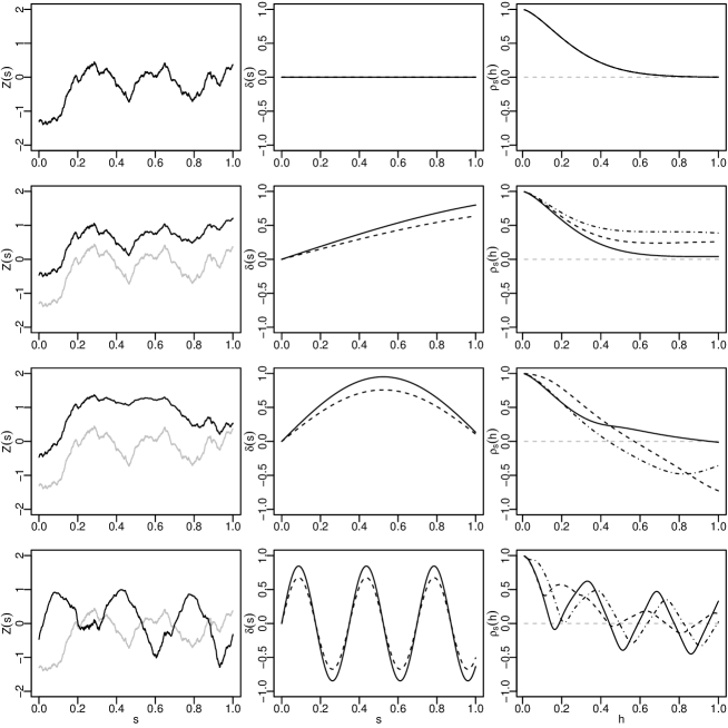
Figure 1: Simulations from four univariate skew-normal random processes on $[0,1]$ with $\varepsilon=0$. The left column shows the sample path (solid line) of the simulated process $Z(s)$ and of the generating Gaussian process $X(s)$ (grey line). The middle column illustrates the slant function $\delta(s)$ (solid line) and the mean $m(s)$ of the process (dashed line). The right column displays the non-stationary correlation functions at locations $s=0.1$ (solid line), $0.5$ and $0.75$ (dot-dash). Rows 1–3 use slant function $\delta(s)=a\sin(bs)$ with $a=0.95$ and $b=0,1$ and $3$ respectively, whereas row 4 uses $\delta(s)=a^{2}\sin(bs)\cos(bs)$ with $a=1.3$ and $b=0.9$.

The first row shows the standard stationary case. The second row illustrates the non-stationary correlation function obtained with $s=0.1$ (solid line) behaving close to the stationary correlation, however decaying more slowly as $s$ increases and approaching, but not reaching zero exactly. The third row demonstrates both that points may be negatively correlated and that $\rho_{s}(h)$ is not necessarily a decreasing function in $h$. The bottom row highlights this even more clearly – correlation functions need not be monotonically decreasing – implying that pairs of points far apart can be more dependent than nearby points.

Simulating a skew-normal random process is computationally cheap through Definition 2, with the simulation of the required stationary Gaussian process achievable through many fast algorithms (e.g., Wood and Chan, 1994, Chan and Wood, 1997). Rather than relying on (2.2), for practical purposes, to directly simulate from a skew-normal process with given parameters $\alpha$, $\bar{\Omega}$ and $\tau$, a conditioning sampling approach can be adopted (Azzalini, 2013, Ch. 5).

Specifically, let $X(s)$ define a zero-mean, unit variance stationary Gaussian random field on $\mathbb{S}$ with correlation function $\omega(h)={\mathbb{E}}\{X(s)X(s+h)\}$ and let $\bar{\Omega}$ be the $d\times d$ correlation matrix of $X(s_{1}),\ldots,X(s_{d})$. Specify $\alpha:\mathbb{S}\mapsto{\mathbb{R}}$ to be a continuous square-integrable function and let $\langle\alpha,X\rangle=\int_{\mathbb{S}}\alpha(s)X(s)\,\text{d}s$ be the inner product. Let $X^{\prime}$ be a standard normal random variable independent of $X$ and $\tau\in{\mathbb{R}}$. If we define

$$Z(s)=\left\{X(s)|\langle\alpha,X\rangle>X^{\prime}-\tau\right\},\qquad s\in\mathbb{S}$$ (12)

then, for any finite set $s_{1},\ldots,s_{d}\in\mathbb{S}$, the distribution of $Z(s_{1}),\ldots,Z(s_{d})$ is $\mathcal{S}\mathcal{N}(\bar{\Omega},\alpha,\tau)$, where $\alpha\equiv\{\alpha(s_{1}),\ldots,\alpha(s_{d})\}$. For simplicity we also refer to $\alpha(s)$ as the slant function. More efficient simulation of skew-normal processes can be achieved by considering the form $Z(s)=X(s)$ if $\langle\alpha,X\rangle>X^{\prime}-\tau$ and $Z(s)=-X(s)$ otherwise (e.g. Azzalini, 2013, Ch. 5).

We conclude this section by discussing some extremal properties of the skew-normal process $Z(s)$. For a finite sequence of points $s_{1},\ldots,s_{d}\in\mathbb{S}$, with $d\geq 2$. Each margin $Z(s_{i})$ follows a skew-normal distribution (Azzalini, 2013) and so is in the domain of attraction of a Gumbel distribution (Chang and Genton, 2007, Padoan, 2011). Further, each pair $(Z(s_{i}),Z(s_{j}))$ is asymptotically independent (Bortot, 2010, Lysenko et al., 2009). However, in this case a broad class of tail behaviours can still be obtained by assuming that the joint survival function is regularly varying at $+\infty$ with index $-1/\eta$ (Ledford and Tawn, 1996), so that

$$\text{Pr}(Z(s_{i})>x,Z(s_{j})>x)=x^{-1/\eta}\,\mathscr{L}(x),\qquad x\rightarrow+\infty,$$ (13)

where $\eta\in(0,1]$ is the coefficient of tail dependence and $\mathscr{L}(x)$ is a slowly varying function i.e., $\mathscr{L}(ax)/\mathscr{L}(x)\rightarrow 1$ as $x\rightarrow+\infty$, for fixed $a>0$. Considering $\mathscr{L}$ as a constant, at extreme levels margins are negatively associated when $\eta<1/2$, independent when $\eta=1/2$ and positively associated when $1/2<\eta<1$. When $\eta=1$ and $\mathscr{L}(x)\nrightarrow 0$ asymptotic dependence is obtained. We derive the asymptotic behavior of the joint survival function (13) for a pair of skew-normal margins. As our primary interest is in spatial applications, we focus on the joint upper tail of the skew-normal distribution when the variables are positively correlated or uncorrelated.

Proposition 4.

Let $Z\sim\mathcal{S}\mathcal{N}_{2}(\bar{\Omega},\alpha)$, where $\alpha=(\alpha_{1},\alpha_{2})^{\top}$ and $\bar{\Omega}$ is a correlation matrix with off-diagonal term $\omega\in[0,1)$. The joint survivor function of the bivariate skew-normal distribution with unit Fréchet margins behaves asymptotically as (13), where:

1. when either $\alpha_{1},\alpha_{2}\geq 0$, or $\omega>0$ and $\alpha_{j}\leq 0$ and $\alpha_{3-j}\geq-\omega^{-1}\alpha_{j}$ for $j=1,2$, then

   $\eta=(1+\omega)/2$,   $\mathscr{L}(x)=\frac{2\,(1+\omega)}{1-\omega}(4\pi\log x)^{-\omega/(1+\omega)};$

2. when $\omega>0$, $\alpha_{j}<0$, and $-\omega\,\alpha_{j}\leq\alpha_{3-j}<-\omega^{-1}\alpha_{j}$, for $j=1,2$, then

   1. If $\alpha_{3-j}>-\alpha_{j}/\bar{\alpha}_{j}$ then

      $\eta=\frac{(1-\omega^{2})\bar{\alpha}_{j}^{2}}{1-\omega^{2}+(\bar{\alpha}_{j}-\omega)^{2}}$,  $\mathscr{L}(x)=\frac{2\,\bar{\alpha}_{j}^{2}(1-\omega^{2})}{(\bar{\alpha}_{j}^{2}-\omega)(1-\omega\bar{\alpha}_{j})}(4\pi\log x)^{1/2\eta-1};$

   2. If $\alpha_{3-j}<-\alpha_{j}/\bar{\alpha}_{j}$ then

      $\eta=\left[\frac{1-\omega^{2}+(\bar{\alpha}_{j}-\omega)^{2}}{(1-\omega^{2})\bar{\alpha}_{j}^{2}}+\left(\alpha_{3-j}+\frac{\alpha_{j}}{\bar{\alpha}_{j}}\right)^{2}\right]^{-1}$,

      $\mathscr{L}(x)=\frac{-2^{3/2}\pi^{1/2}\bar{\alpha}_{j}^{2}(1-\omega^{2})(\alpha_{3-j}+\alpha_{j}/\bar{\alpha}_{j})^{-1}}{(\bar{\alpha}_{j}-\omega)\{1-\omega\bar{\alpha}_{j}+\alpha_{j}(\alpha_{j}+\alpha_{3-j}\bar{\alpha}_{j})(1-\omega^{2})\}}(4\pi\log x)^{1/2\eta-3/2};$

3. when either $\alpha_{1},\alpha_{2}<0$, or $\omega>0$, $\alpha_{j}<0$ and $0<\alpha_{3-j}<-\omega\,\alpha_{j}$ for $j=1,2$, then

   $\eta=\left\{\frac{1}{1-\omega^{2}}\left(\frac{\alpha_{3-j}^{2}(1-\omega^{2})+1}{\bar{\alpha}_{3-j}^{2}}+\frac{\alpha_{j}^{2}(1-\omega^{2})+1}{\bar{\alpha}_{j}^{2}}+\frac{2(\alpha_{3-j}\alpha_{j}(1-\omega^{2})-\omega)}{\bar{\alpha}_{3-j}\bar{\alpha}_{j}}\right)\right\}^{-1}$,

   $\mathscr{L}(x)=\frac{-2^{3/2}\pi^{1/2}\bar{\alpha}_{j}^{3/2}\bar{\alpha}_{3-j}^{2}(1-\omega^{2})(\alpha_{i}\bar{\alpha}_{j}+\alpha_{j}\bar{\alpha}_{3-j})^{-1}}{(\bar{\alpha}_{j}-\omega\bar{\alpha}_{3-j})\{1-\omega\bar{\alpha}_{j}+\alpha_{j}(\alpha_{j}+\alpha_{3-j}\bar{\alpha}_{j}/\bar{\alpha}_{3-j})(1-\omega^{2})\}}(4\pi\log x)^{1/2\eta-3/2};$

where $\bar{\alpha}_{j}=\sqrt{1+\alpha^{*2}_{j}}$ and $\alpha^{*}_{j}:=\alpha^{*}_{\{j\}}=\frac{\alpha_{j}+\omega\alpha_{3-j}}{\sqrt{1+\alpha_{3-j}(1-\omega^{2})}}.$

Proof in Appendix A.3.

As a result, when both marginal parameters are non-negative (case 1) then $1/2\leq\eta<1$, with $\eta=1/2$ occurring when $\omega=0$. As a consequence, as for the Gaussian distribution (for which $\alpha=0$) the marginal extremes are either positively associated or exactly independent. The marginal extremes are also completely dependent when $\omega=1$, regardless of the values of the slant parameters, $\alpha$. When one marginal parameter is positive and one is negative (case 2) then $\eta>(1+\omega)/2$. In this case the extreme marginals are also positively associated, but the dependence is greater than when the random variables are normally distributed. Finally, when both marginal parameters are negative (case 3), then $0<\eta<1/2$ implying that the extreme marginals are negatively associated, although $\omega>0$. It should be noted that differently from the Gaussian case ($\alpha=0$) where $\omega>0$ implies a positive association, in this case it is not necessarily true. In summary, the degree of dependence in the upper tail of the skew-normal distribution ranges from negative to positive association and including independence.

3 Spectral representation for the extremal-skew-$t$ process

The spectral representation of stationary max-stable processes with common unit Fréchet margins can be constructed using the fundamental procedures introduced by de Haan (1984) and Schlather (2002) (see also de Haan and Ferreira, 2006, Ch. 9). This representation can be formulated in broader terms resulting in max-stable processes with $\nu$-Fréchet univariate marginal distributions, with $\nu>0$ (Opitz, 2013). In order to state our result we rephrase the spectral representation so to also take into account non-stationary processes.

Let $\{Y(s)\}_{s\in\mathbb{S}}$ be a non-stationary real-valued stochastic process with continuous sample path on $\mathbb{S}$ such that ${\mathbb{E}}\left\{\sup_{s\in\mathbb{S}}Y(s)\right\}<\infty$ and $m^{+}(s)={\mathbb{E}}[\{Y^{+}(s)\}^{\nu}]<\infty,\forall s\in\mathbb{S}$ for $\nu>0$, where $Y^{+}(\cdot)=\max\{Y(\cdot),0\}$ denotes the positive part of $Y$. Let $\{R_{i}\}_{i\geq 1}$ be the points of an inhomogeneous Poisson point process on $(0,\infty)$ with intensity $\nu r^{-(\nu+1)}$, $\nu>0$, which are independent of $Y$. Define

$$U(s)=\max_{i=1,2,\ldots}\{R_{i}Y_{i}^{+}(s)\}/\{m^{+}(s)\}^{1/\nu},\quad s\in\mathbb{S},$$ (14)

where $Y_{1},Y_{2},\ldots$ are iid copies of $Y$. Then $U$ is a max-stable process with common $\nu$-Fréchet univariate margins. In particular, for fixed $s\in\mathbb{S}$ and $x(s)>0$ we have

$$\text{Pr}(U(s)\leq x(s))=\exp\left[-\frac{{\mathbb{E}}\{Y^{+}(s)\}^{\nu}}{x^{\nu}(s)m^{+}(s)}\right]=\exp\{-1/x^{\nu}(s)\},$$

and for fixed $s_{1},\ldots,s_{d}$ the finite dimensional distribution of $U$ has exponent function

$$V(x(s_{1}),\ldots,x(s_{d}))={\mathbb{E}}\left(\max_{j}\left[\frac{\{Y^{+}(s_{j})/x(s_{j})\}^{\nu}}{m^{+}(s_{j})}\right]\right),\quad x(s_{j})>0,\,j=1,\ldots,d$$ (15)

(de Haan and Ferreira, 2006, Ch. 9).

In this construction, the impact of a non-stationary process $Y(s)$ would be that the dependence structure of the max-stable process $U(s+h)$ depends on both the separation $h$ and the location $s\in\mathbb{S}$, and would therefore itself be non-stationary. The below theorem derives a max-stable process $U(s)$ when $Y(s)$ is the skew-normal random field introduced in Section 2.2.

Theorem 1 (Extremal skew-$t$ process).

Let $Y(s)$ be a skew-normal random field on $s\in\mathbb{S}$ with finite dimensional distribution $\mathcal{S}\mathcal{N}_{d}(\bar{\Omega},\alpha,\tau)$, as defined in equation (12). Then the max-stable process $U(s)$, given by (14), has $\nu$-Fréchet univariate marginal distributions and exponent function

$$V(x_{j},j\in I)=\sum_{j=1}^{d}x_{j}^{-\nu}\Psi_{d-1}\left(\left(\sqrt{\frac{\nu+1}{1-\omega^{2}_{i,j}}}\left(\frac{x^{\circ}_{i}}{x^{\circ}_{j}}-\omega_{i,j}\right),i\in I_{j}\right)^{\top};\bar{\Omega}^{\circ}_{j},\alpha^{\circ}_{j},\tau^{\circ}_{j},\kappa^{\circ}_{j},\nu+1\right),$$ (16)

where $x_{j}\equiv x(s_{j})$, $\Psi_{d-1}$ is a $(d-1)$-dimensional non-central extended skew-$t$ distribution (Definition 1) with correlation matrix $\bar{\Omega}^{\circ}_{j}$, shape, extension and non-centrality parameters $\alpha^{\circ}_{j},\tau^{\circ}_{j}$ and $\kappa^{\circ}_{j}$, $\nu+1$ degrees of freedom, $I=\{1,\ldots,d\}$, $I_{j}=I\backslash\{j\}$, and $\omega_{i,j}$ is the $(i,j)$-th element of $\bar{\Omega}$.

Proof (and further details) in Appendix A.4.

We call the process $U(s)$ with exponent function (16) an extremal skew-$t$ process.

Note that in Theorem 1 when $\tau=0$, and the slant function is such that $\alpha(s)\equiv 0$ for all $s\in\mathbb{S}$, then the exponent function (16) becomes

$$V(x_{j},j\in I)=\sum_{j\in I}x_{j}^{-\nu}\Psi_{d-1}\left[\left(\sqrt{\frac{\nu+1}{1-\omega^{2}_{i,j}}}\left(\frac{x_{i}}{x_{j}}-\omega_{i,j}\right),i\in I_{j}\right)^{\top};\bar{\Omega}^{\circ}_{j},\nu+1\right].$$ (17)

This is the exponent function of the extremal-$t$ process as discussed in Opitz (2013).

If we assume $\tau=0$ in (12), then the bivariate exponent function of the extremal skew-$t$ process seen as a function of the separation $h$ is equal to

$$V\{x(s),x(s+h)\}=\frac{\Psi(b(x^{*}_{s}(h));\alpha^{*}_{s}(h),\tau^{*}_{s}(h),\nu+1)}{x^{\nu}(s)}+\frac{\Psi(b(x^{+}_{s}(h));\alpha^{+}_{s}(h),\tau^{+}_{s}(h),\nu+1)}{x^{\nu}(s+h)}$$

where $\Psi$ is a univariate extended skew-$t$ distribution, $b(\cdot)=\sqrt{\frac{\nu+1}{1-\omega^{2}(h)}}(\cdot-\omega(h)),$

$$\begin{array}[]{rclrcl}x^{*}_{s}(h)&=&\frac{x(s+h)\Gamma_{s}(h)}{x(s)},&x^{+}_{s}(h)&=&\frac{x(s)}{x(s+h)\Gamma_{s}(h)},\\ \\ \alpha^{*}_{s}(h)&=&\alpha(s+h)\sqrt{1-\omega^{2}(h)},&\alpha_{s}^{+}(h)&=&\alpha(s)\sqrt{1-\omega^{2}(h)},\\ \\ \tau_{s}^{*}(h)&=&\sqrt{\nu+1}\{\alpha(s)+\alpha(s+h)\omega(h)\},&\tau_{s}^{+}(h)&=&\sqrt{\nu+1}\{\alpha(s+h)+\alpha(s)\omega(h)\},\\ \end{array}$$

and

$$\Gamma_{s}(h)=\left(\frac{\Psi\left[\alpha(s)+\alpha(s+h)\omega(h)\sqrt{\frac{\nu+1}{\alpha^{2}(s+h)\{1-\omega^{2}(h)\}}};\nu+1\right]}{\Psi\left[\alpha(s+h)+\alpha(s)\omega(h)\sqrt{\frac{\nu+1}{\alpha^{2}(s)\{1-\omega^{2}(h)\}}};\nu+1\right]}\right)^{1/\nu}.$$

Clearly, as the dependence structure depends on both correlation function $\omega(h)$ and the slant function $\alpha(s)$, and therefore on the value of $s\in\mathbb{S}$, it is a non-stationary dependence structure. From the bivariate exponent function we can derive the non-stationary extremal coefficient function, using the relation $\theta_{s}(h)=V(1,1)$, which gives

$$\theta_{s}(h)=\Psi(b(\Gamma_{s}(h));\alpha^{*}_{s}(h),\tau^{*}_{s}(h),\nu+1)+\Psi(b(1/\Gamma_{s}(h));\alpha^{+}_{s}(h),\tau^{+}_{s}(h),\nu+1).$$ (18)

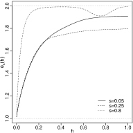
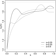
Figure 2: Examples of univariate ($k=1$) non-stationary isotropic extremal coefficient functions $\theta_{s}(h)$, for the extremal skew-$t$ process over $s\in[0,1]$, using correlation function (11) where $h\in[0,1]$, $\lambda=1.5$ and $\gamma=0.3$. Slant functions are (left to right panels): $\alpha(s)=-1-s+\exp\{\sin(5s)\},\alpha(s)=1+1.5s-\exp\{\sin(8s)\}$ and $\alpha(s)=2.25\sin(9s)\cos(9s)$. Solid, dashed and dot-dashed lines represent the fixed locations $s=0.05,0.25$ and $0.8$ respectively.

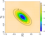
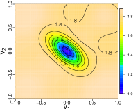
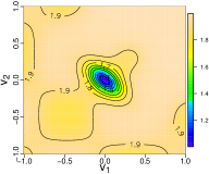
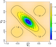
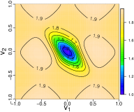
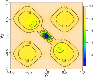
Figure 3: Bivariate ($k=2$) geometric anisotropic non-stationary extremal coefficient functions $\theta_{s}(h)$, for the extremal skew-$t$ process on $s\in[0,1]^{2}$, based on extremal coefficient function (18) with $\lambda=1.5$ and $\gamma=0.3,$ where $h=v^{\top}Rv$, $v=(v_{1},v_{2})^{\top}\in[-1,1]^{2}$ and $R$ is a $2\times 2$ matrix whose diagonal elements are $2.5$ and off-diagonal elements $1.5$. Slant functions are $\alpha(s)=\exp\{\sin(4s_{1})\sin(4s_{2})-s_{1}s_{2}-1\}$ (top panels) and $\alpha(s)=2.25\{\sin(3s_{1})\cos(3s_{1})+\sin(3s_{2})\cos(3s_{2})\}$ (bottom), with $s=(s_{1},s_{2})^{\top}\in[0,1]^{2}$. Left to right, panels are based on fixing $s=(0.2,0.2)^{\top}$, $s=(0.4,0.4)^{\top}$ and $s=(0.85,0.85)^{\top}$ (top panels) and $s=(0.25,0.25)^{\top}$, $s=(0.25,0.8)^{\top}$ and $s=(0.8,0.8)^{\top}$ (bottom).

Figure 2 shows some examples of univariate ($k=1$) non-stationary isotropic extremal coefficient functions obtained from (18) using the power-exponential correlation function (11). Each panel illustrates a different slant function $\alpha(s)$, with the line-types indicating the fixed location value of $s\in\mathbb{S}.$ The extremal coefficient functions $\theta_{s}(h)$ increase as the value of $h$ increases, meaning that the dependence of extremes decreases with the distance. $\theta_{s}(h)$ grows with different rates depending on the location $s\in\mathbb{S}$. Although the ergodicity and mixing properties of the process must be investigated, numerical results show that for some $s$, $\theta_{s}(h)\rightarrow 2$ as $|h|\rightarrow+\infty$. By increasing the complexity of the slant function (e.g. centre and right panels) it is possible to construct extremal coefficient functions which exhibit stronger dependence for larger distances, $h$, compared to shorter distances. Similarly Figure 3 illustrates examples of bivariate ($k=2$) non-stationary geometric anisotropic extremal coefficient functions, $\theta_{s}(h)$, also obtained from (18). Similar interpretations to the univariate case can be made (Figure 2), in addition to noting that the level of dependence is affected by the direction (from the origin).

4 Inference for extremal skew-$t$ processes

Parametric inference for the extremal-skew-$t$ process can be performed in two ways. The first uses the marginal composite-likelihood approach (e.g. Padoan et al., 2010, Davison and Gholamrezaee, 2012, Huser and Davison, 2013), since only marginal densities of dimension up to $d=4$ are practically available (see the Supporting Information).

Let $\vartheta\in\Theta\subseteq\mathbb{R}^{p}$, $p=1,2,\ldots$, denote the vector of dependence parameters of the extremal-skew-$t$ process. Consider a sample $(x_{i},i=1,\ldots,n$) with $x_{i}\in\mathbb{R}^{d}_{+}$ of $n$ iid replicates of the process observed over a finite number of points $(s_{j},j\in I)$ with $s_{j}\in\mathbb{S}$. For simplicity, it is assumed that the univariate marginal distributions are unit Fréchet. The pairwise or triplewise ($m=2,3$) log-composite-likelihood is defined by

$$\ell_{m}(\vartheta;x)=\sum_{i=1}^{n}\sum_{E\in E_{m}}\log f(x_{i}\in E;\vartheta),\quad m=2,3,$$

where $x=(x_{1},\ldots,x_{n})^{\top}$ with $x_{i}\in\mathbb{R}_{+}^{m}$ and $f$ is a marginal extremal-skew-$t$ pdf associated with each member of a set of marginal events $E_{m}$. See e.g. Varin et al. (2011) for a complete description of composite likelihood methods.

A second approach is to use the approximate likelihood function introduced by Coles and Tawn (1994), which is constructed on the space of angular densities. The angular measure of the extremal-skew-$t$ dependence model (16) places mass on the interior as well as on all the other subspaces of the simplex, such as the edges and the vertices. We derive some of these densities following the results in Coles and Tawn (1991).

Let $J$ be an index set that takes values in $\mathbb{I}=\mathbb{P}(\{1,\ldots,d\})\backslash\emptyset$, where $\mathbb{P}(I)$ is the power set of $I$. For any fixed $d$ and all $J\in\mathbb{I}$, the sets

$$\mathbb{W}_{d,J}=(w\in\mathbb{W}:w_{j}=0,\text{ if }j\notin J;\,w_{j}>0\text{ if }j\in J)$$

provide a partition of the $d$-dimensional simplex $\mathbb{W}$ into $2^{d}-1$ subsets. Let $k=|J|$ be the size of $J$. Let $h_{d,J}$ denote the density that lies on the subspace $\mathbb{W}_{d,J}$, which has $k-1$ free parameters $w_{j}$ such that $j\in J$. When $J=\{1,\ldots,d\}$ the angular density in the interior of the simplex is

$$h(w)=\frac{\psi_{d-1}\left(\left[\sqrt{\frac{\nu+1}{1-\omega_{i,1}^{2}}}\left\{\left(\frac{w^{\circ}_{i}}{w^{\circ}_{1}}\right)^{1/\nu}-\omega_{i,1}\right\},i\in I_{1}\right]^{\top};\Omega_{1}^{\circ},\alpha_{1}^{\circ},\tau_{1}^{\circ},\kappa_{1}^{\circ},\nu+1\right)}{w_{1}^{(d+1)}\left\{\prod_{i=2}^{d}\frac{1}{\nu}\sqrt{\frac{\nu+1}{1-\omega_{i,1}^{2}}}\Big{(}\frac{w^{\circ}_{i}}{w^{\circ}_{1}}\Big{)}^{\frac{1}{\nu}-1}\frac{m_{i}^{+}}{m_{1}^{+}}\right\}^{-1}},\quad w\in\mathbb{W}$$ (19)

where $\psi_{d-1}$ denotes the $d-1$-dimensional skew-$t$ density, $I_{j}=\{1,\ldots,d\}\backslash j$ and where the parameters $\Omega_{1}^{\circ},\alpha_{1}^{\circ},\tau_{1}^{\circ},\kappa_{1}^{\circ}$ and $w^{\circ}_{i}=w_{i}(m_{i}^{+})^{1/\nu}$ are given in the proof to Theorem 1 (Appendix A.4). When $J=\{i_{1},\ldots,i_{k}\}\subset\{1,\ldots,d\}$, the angular density for any $x\in{\mathbb{R}}^{d}_{+}$ is

$$h_{d,J}\left(\frac{x_{i_{1}}}{\sum_{\begin{subarray}{c}i\in J\end{subarray}}x_{i}},\cdots,\frac{x_{i_{k-1}}}{\sum_{i\in J}x_{i}}\right)=-\left(\sum_{\begin{subarray}{c}i\in J\end{subarray}}x_{i}\right)^{k+1}\lim_{\begin{subarray}{c}x_{j}\rightarrow 0,\\ j\notin J\end{subarray}}\frac{\partial^{k}V}{\partial x_{i_{1}}\cdots\partial x_{i_{k}}}(x).$$ (20)

Thus, when $J=\{j\}$ for any $j\in\{1,\ldots,d\}$ then $\mathbb{W}_{d,J}$ is a vertex ${\bf e}_{j}$ of the simplex and the density is a point mass, denoted $h_{d,J}=H(\{{\bf e}_{j}\})$. In this case (20) reduces to

$$h_{d,J}=\Psi_{d-1}\left\{\left(-\sqrt{\frac{\nu+1}{1-\omega_{i,j}^{2}}}\omega_{i,j},{i\in I_{j}}\right)^{\top};\Omega^{\circ}_{j},\alpha_{j}^{\circ},\tau_{j}^{\circ},\kappa_{j}^{\circ},\nu+1\right\},$$ (21)

where $\Psi_{d-1}$ denotes the $d-1$-dimensional skew-$t$ distribution with parameters again given in the proof to Theorem 1 (Appendix A.4).

Computations of all $2^{d}-1$ densities that lie on the edges and vertices of the simplex are available for $d=3$. In this case, the angular densities on the interior and vertices of the simplex can be deduced from (19) and (21). For all $i,j\in J=\{1,2,3\}$, with $i\neq j$, the angular density on the edges of $\mathbb{W}_{d,J}$ for $w\in\mathbb{W}_{d,J}$ is given by

$$h_{3,\{i,j\}}(w) =\sum_{u,v\in\{i,j\},u\neq v}\left(\frac{\psi(b_{u,v}^{\circ};\nu+1)}{\Psi(\bar{\tau}_{u};\nu+1)}\Psi_{2}\left[\left\{y_{1}^{\circ}(u,v),y_{2}^{\circ}(u,v)\right\}^{\top};\bar{\Omega}^{\circ\circ}_{u},\nu+2\right]\right.$$

$$\qquad\times\frac{1}{w}_{1}\left\{\frac{\text{d}^{2}b_{u,v}^{\circ}}{\text{d}w_{u}\text{d}w_{v}}+\frac{\text{d}b_{u,v}^{\circ}}{\text{d}w_{v}}\left(\frac{\text{d}b_{u,v}^{\circ}}{\text{d}w_{u}}\frac{(\nu+2)b_{u,v}^{\circ}}{\nu+1+b_{u,v}^{\circ 2}}-\frac{1}{w}_{1}\right)\right\}$$

$$\qquad+\psi\{y_{1}^{\circ}(u,v);\nu+2\}\sqrt{\frac{\nu+2}{1-\Omega^{\circ 2}_{u,[1,2]}}}\frac{b_{u,v}^{\circ}c_{u,\bar{k}}+\Omega^{\circ 2}_{u,[1,2]}(\nu+1)}{(\nu+1+b_{u,v}^{\circ 2})^{3/2}}$$

$$\qquad\times\Psi\left(\frac{\sqrt{\nu+3}\left\{z_{2}^{\circ}(u,v)\Omega^{\circ\circ}_{u,[1,1]}-z_{1}^{\circ}(u,v)\Omega^{\circ\circ}_{u,[1,2]}\right\}}{\sqrt{\left[\Omega^{\circ\circ}_{u,[1,1]}\{\nu+1+b_{u,v}^{\circ 2}\}+z_{1}^{\circ 2}(u,v)\right]\det(\Omega^{\circ\circ}_{u})}};\nu+3\right)$$ (22)

$$\qquad+\psi\{y_{2}^{\circ}(u,v);\nu+2\}\sqrt{\frac{\nu+2}{1-\Omega^{*2}_{u,[1,3]}}}\frac{x(u,v)\bar{\tau}_{u}+\Omega^{*2}_{u,[1,3]}(\nu+1)}{\{\nu+1+b_{u,v}^{\circ 2}\}^{3/2}}$$

$$\qquad\left.\times\Psi\left\{\frac{\sqrt{\nu+3}\left\{z_{1}^{\circ}(u,v)\Omega^{\circ\circ}_{u,[2,2]}-z_{2}^{\circ}(u,v)\Omega^{\circ\circ}_{u,[1,2]}\right\}}{\sqrt{\left(\Omega^{\circ\circ}_{u,[2,2]}\{\nu+1+b_{u,v}^{\circ 2}\}+z_{2}^{\circ}(u,v)^{2}\right)\det(\Omega^{\circ\circ}_{u})}};\nu+3\right\}\right),$$

where for all $u,v\in J$, with $u\neq v$, and $\bar{k}\notin\{i,j\}$,

$$y_{\ell}^{\circ}(u,v)=\frac{z_{\ell}^{\circ}(u,v)}{\sqrt{\Omega_{u,[\ell,\ell]}^{\circ}}}\sqrt{\frac{\nu+2}{\nu+1+b_{u,v}^{\circ 2}}},\;\ell=1,2,\quad z_{1}^{\circ}(u,v)=c_{u,\bar{k}}-\Omega^{\circ}_{u,[1,2]}b_{u,v}^{\circ},$$

$$c_{u,v}=-\omega_{u,v}\sqrt{\frac{\nu+1}{1-\omega^{2}_{u,v}}},\quad z_{2}^{\circ}(u,v)=\bar{\tau}_{u}-\Omega^{\circ}_{u,[1,3]},\quad b_{u,v}^{\circ}=\sqrt{\frac{\nu+1}{1-\omega^{2}_{u,v}}}\left(\left(\frac{w_{v}^{\circ}}{w_{u}^{\circ}}\right)^{1/\nu}-\omega_{u,v}\right),$$

$$\quad\Omega^{\circ}_{u}=\left[\begin{array}[]{cc}\bar{\Omega}_{u}&-\delta_{u}\\ -\delta_{u}^{\top}&1\end{array}\right],\quad\delta_{u}^{\top}=\bar{\Omega}_{u}\left(\alpha_{v}\sqrt{1-\omega_{u,v}^{2}},\alpha_{k}\sqrt{1-\omega_{u,k}^{2}}\right)^{\top},\;\bar{\Omega}^{\circ\circ}_{u}={\omega_{u}^{\circ}}^{-1/2}\Omega^{\circ\circ}_{u}{\omega_{u}^{\circ}}^{-1/2},$$

$\omega_{u}^{\circ}=\mbox{diag}(\Omega^{\circ\circ}_{u})$, $\Omega^{\circ\circ}_{u}=\Omega^{\circ}_{u,[-1,-1]}-\Omega^{\circ}_{u,[-1,1]}\Omega^{\circ}_{u,[1,-1]}$. Components of $\Omega^{\circ}_{u}$ and $\Omega^{\circ\circ}_{u}$ are respectively given by $\Omega^{\circ}_{u,[i,j]}$ and $\Omega^{\circ\circ}_{u,[i,j]}$ for $i,j\in J$. See also Appendix A.4 for further details. When, $\tau=0$ and $\alpha(s)=0$, then the densities (19), (21) and (4) reduce to the densities of the extremal-$t$ dependence model. A graphical illustration that shows the difference between the two dependence models is provided in the Supporting Information.

Therefore, for $d=3$ the estimation of dependence parameters can be based on the following approach. Let $\{(r_{i},w_{i}):i=1,\ldots,n\}$ be the set of observations, where $r_{i}=\sum_{j\in I}x_{i,j}$ and $w_{i}=x_{i}/r_{i}$, with $x_{i}=(x_{i,j})_{j\in I}$, are pseudo-polar radial and angular components. Then the approximate log-likelihood is defined by

$$\ell(\vartheta;\tilde{w})=\sum_{\begin{subarray}{c}i=1,\ldots,n:\\ r_{i}>r_{0}\end{subarray}}\log h(w_{i};\vartheta),$$ (23)

where $\tilde{w}=(w_{1},\ldots,w_{n})^{\top}$, for some radial threshold $r_{0}>0$, and where $h$ is the angular density function of the extremal-skew-$t$ dependence model. The components of the sum in (23) comprise the three types of angular densities lying on the interior, edges and vertices of the simplex. Whether an angular component belongs either to the interior, an edge or a vertex of the simplex, producing the associated density, is determined according the following criterion. We select a threshold $c\in[0,0.1]$ and we construct the following partitions for an arbitrary observation $w_{i}=(w_{i,j},w_{i,k},w_{i,l})$, $i=1,\ldots,n$. Set $w\equiv w_{i}$ for simplicity. When $\mathcal{C}_{j}=\{w_{j}>1-c;j\in I\}$ then an observation belongs to vertex $\boldsymbol{e}_{j}$. When $\mathcal{E}_{j,k}=\{w_{j},w_{k}<1-c,w_{l}<c,w_{j}>1-2w_{k},w_{k}>1-2w_{j};j\in I,k\in I_{j},l\in I_{j}\backslash\{k\}\}$, then an observation belongs to edge between the $j$th and $k$th components. When $\mathcal{I}=\{w_{j}>c;j\in I\}$ then an observation belongs to the interior (see the Supporting Information for more details). The components of the angular density $h(w)$ then require rescaling so that they satisfy the constraints of valid angular densities – namely that they integrate to the number of components of $w$ (3 in the trivariate case) – while also respecting the partition of $\mathbb{W}$ implied by $c$. Without this rescaling then the likelihood of e.g. the model that places mass on all subsets of the simplex is not comparable with that of models that places mass only on subsets of the simplex. Specifically

$$\int_{\mathbb{W}}h(w)\text{d}w=K_{\mathcal{C}}\sum_{j\in I}\int_{\mathcal{C}_{j}}h_{3,\{j\}}\text{d}w+\sum_{\begin{subarray}{c}j=1,2\;\\ k=j+1,3\end{subarray}}K_{\mathcal{E}_{j,k}}\int_{\mathcal{E}_{j,k}}h_{3,\{j,k\}}(w)\text{d}w+K_{\mathcal{I}}\int_{\mathcal{I}}h_{3,\{1,2,3\}}(w)\text{d}w=3,$$

where

$$K_{\mathcal{C}}=\frac{4}{\sqrt{3}c^{2}},\quad K_{\mathcal{E}_{j,k}}=\frac{2\int_{0}^{1}h_{3,\{j,k\}}(w)\text{d}w}{c\sqrt{3}(1-2c)},\quad K_{\mathcal{I}}=\frac{\int_{0}^{1}\int_{0}^{1}h_{3,\{1,2,3\}}(w)\text{d}w}{\int_{c}^{1-2c}\int_{c}^{1-2c}h_{3,\{1,2,3\}}(w)\text{d}w},$$

and $h_{3,\{j\}}$, $h_{3,\{j,k\}}(w)$ and $h_{3,\{1,2,3\}}(w)$ are defined above. Note that for $j,k\in I$ with $j\neq k$, we have that $h_{3,\{j,k\}}(w)=h_{3,\{k,j\}}(w)$. In the bivariate case ($d=2$), the appropriate modification only considers the mass on the vertices and interior.

We now illustrate the ability of the approximate likelihood in estimating the extremal dependence parameters in the bivariate and trivariate cases. We generate $500$ replicate datasets of sizes $5000$ (bivariate) and $1000$ (trivariate), with parameters $\vartheta_{2}=(\omega,\nu)=(0.6,1.5)$ and $\vartheta_{3}=(\omega_{1,2},\omega_{1,3},\omega_{2,3},\nu)=(0.6,0.8,0.7,1)$. Each dataset is transformed to pseudo-polar coordinates and the 100 observations with the largest radial component are retained. Parameters are estimated through the profile likelihood where the dependence parameter $\omega$ is the parameter of interest and the degree of freedom $\nu$ is considered as a nuisance parameter. Parameters are estimated for different values of the threshold $c=0,0.02,0.04,0.06,0.08,0.1$. In order to compare likelihoods for different values of $c$, the likelihood functions are evaluated using those data points considered to belong to the interior of the simplex, multiplied by the mass at the corners and/or edges in proportion to their rescaling constants.

Figure 4: Left to right: Boxplots of the estimates of the dependence parameter $\omega$, the degree of freedom $\nu$ and the associated maximum of the likelihood function based on the rescaled angular density, when $c=0,0.02,0.04,0.06,0.08$ and $0.1$. Boxplots are constructed from $500$ replicate datasets of size 5000. Horizontal lines indicate the true values $\omega=0.6$ and $\nu=1.5$.

Figures 4 and 5 provide (left to right) boxplots of the resulting estimates of the dependence parameter(s) $\omega$, the degree of freedom $\nu$ and of the likelihood function for increasing values of $c$, for the 500 replicate datasets for both bivariate and trivariate cases. The true parameter values are indicated by the horizontal lines.

Figure 5: Left to right: Boxplots of the estimates of the dependence parameter $\omega=(\omega_{1,2},\omega_{1,3},\omega_{2,3})$, the degree of freedom $\nu$ and the associated maximum of the likelihood function based on the rescaled angular density, when $c=0,0.02,0.04,0.06,0.08$ and $0.1$. Boxplots are constructed from 500 replicate datasets of size 1000. Horizontal lines indicate the true values $\omega_{1,2}=0.6,\omega_{1,3}=0.7,\omega_{2,3}=0.7$ and $\nu=1$.

In the rightmost panel of each Figure, the largest values of the log-likelihood are globally obtained for $c=0.02$, for which the most accurate estimates of $\omega$ and $\nu$ are also obtained. Conditional on $c=0.02$ the mean estimates are $\hat{\omega}=0.55$ and $\hat{\nu}=1.79$ in the bivariate case and $\hat{\omega}=(0.62,0.80,0.71)$ and $\hat{\nu}=1.27$ in the trivariate case. Note that the degree of freedom $\nu$ appears to be slightly overestimated, and appears to be better estimated for slightly larger values of $c$. Overall this procedure appears capable of efficiently estimating the model parameters. Note that increased precision of estimates can be obtained by considering a denser range of threshold values $c$.

An independent study comparing the efficiency of the maximum pairwise and triplewise composite likelihood estimators is provided in the Supporting Information.

5 Application to wind speed data

We illustrate the use of the extremal skew-$t$ process using wind speed data (the weekly maximum wind speed in km/h), collected from 4 monitoring stations across Oklahoma, USA, over the March-May period during 1996–2012, as part of a larger dataset of 99 stations. An analysis establishing the significant marginal, station-specific skewness of these data is presented in the Supporting Information. Here, we focus on the dependence structure between stations, where for simplicity the data is marginally transformed to unit Fréchet distributions. Only extremal-$t$ and extremal skew-$t$ models are considered, and parameter estimation is performed via pairwise composite likelihoods as detailed at the beginning of Section 4.

Model comparison is performed through the composite likelihood information criterion (CLIC; Varin et al., 2011) given by

$$\textrm{CLIC}=-2\left[\ell_{2}(\hat{\vartheta};x)-\mathrm{tr}\{\hat{J}(\hat{\vartheta})\hat{H}(\hat{\vartheta})^{-1}\}\right],$$

where $\hat{\vartheta}$ is the maximum composite likelihood estimate of $\vartheta$, $\ell_{2}(\hat{\vartheta};x)$ is the maximised pairwise composite likelihood, and $\hat{J}$ and $\hat{H}$ are estimates of $J(\vartheta)=\mathrm{Var}_{U}(\nabla\ell_{2}(\vartheta;U))$ and $H(\vartheta)={\mathbb{E}}_{U}(-\nabla^{2}\ell_{2}(\vartheta;U))$, the variability and sensibility (hessian) matrices, where $U$ is a bivariate random vector with extremal skew-$t$ distribution.

Stations	Model	$\hat{\omega}$	$\hat{\alpha}$	$\hat{\nu}$	CLIC
(CLOU,CLAY,SALL)	ex-$t$	$(0.67,0.57,0.69)$	$-$	$2.89$	$5395.73$
	ex-skew-$t$	$(0.42,0.74,0.52)$	$(-0.80,2.88,-0.23)$	$2.06$	$5385.07$
			se: $(0.04,0.14,0.03)$
(CLOU,CLAY,PAUL)	ex-$t$	$(0.59,0.50,0.69)$	$-$	$2.53$	$5503.54$
	ex-skew-$t$	$(0.45,0.29,0.65)$	$(-0.68,21.07,23.41)$	$2.16$	$5496.90$
			se: $(0.05,0.97,1.09)$
(CLAY,SALL,PAUL)	ex-$t$	$(0.65,0.61,0.53)$	$-$	$1.55$	$5086.13$
	ex-skew-$t$	$(0.56,0.51,0.39)$	$(3.55,2.36,8.49)$	$1.29$	$5075.87$
			se: $(0.17,0.15,0.63)$
(CLOU,SALL,PAUL)	ex-$t$	$(0.37,0.40,0.42)$	$-$	$1.88$	$5428.04$
	ex-skew-$t$	$(0.29,0.30,0.37)$	$(-0.14,1.04,34.70)$	$2.11$	$5419.27$
			se: $(0.03,0.02,3.49)$

Table 1: Pairwise composite likelihood estimates $\hat{\vartheta}=(\hat{\omega},\hat{\nu})$ and $\hat{\vartheta}=(\hat{\omega},\hat{\alpha},\hat{\nu})$ of the extremal-$t$ (ext-$t$) and extremal skew-$t$ (ex-skew-$t$) models respectively, for all possible triplets of the four locations CLOU, CLAY, PAUL and SALL. Standard errors (se) are shown for $\hat{\alpha}$ only.

Table 1 presents the pairwise composite likelihood estimates of $\omega=(\omega_{12},\omega_{13},\omega_{23})$, $\alpha=(\alpha_{1},\alpha_{2},\alpha_{3})$ and $\nu$ for the extremal-$t$ and extremal skew-$t$ models, obtained for all triplewise combinations of the four locations CLOU, CLAY, PAUL and SALL. For each triple the extremal skew-$t$ model achieves a lower CLIC score than the extremal-$t$ model, indicating its greater suitability. Moreover the standard errors of the estimated slant parameters $\hat{\alpha}$, clearly indicate that these parameters are non-zero, strengthening the argument of a significantly better fit from the extremal skew-$t$ model

For each location triple $(X,Y,Z)$ we can also evaluate the conditional probability of exceeding some fixed threshold $(x,y,z)$ using each parametric model. Table 2 presents estimated probabilities of the two cases $\text{Pr}(X>x|Y>y,Z>z)$ and $\text{Pr}(X>x,Y>y|Z>z),$ along with the associated empirical probabilities and their $95\%$ confidence intervals (CI) for a range of thresholds. For these specific thresholds, the extremal skew-$t$ model provides estimates of the conditional probabilities that fall within the $95\%$ empirical CI. However, four probabilities estimated with the extremal-$t$ model are not consistent with the empirical CI. This indicates that the additional flexibility of the extremal skew-$t$ model allows it to more accurately characterise the dependence structure evident in the observed data.

	Threshold	Extremal-$t$	Extremal skew-$t$	Empirical ($95\%$ CI)
$X|Y,Z$	$(q^{90}_{\textrm{CO}},q^{70}_{\textrm{CA}},q^{70}_{\textrm{PA}})$	$0.2587$	$0.2737$	$0.3333\,(0.2706,0.3960)$
	$(q^{90}_{\textrm{SA}},q^{70}_{\textrm{CA}},q^{70}_{\textrm{PA}})$	$0.3268$	$0.3305$	$0.2973\,(0.2356,0.3590)$
	$(q^{90}_{\textrm{PA}},q^{70}_{\textrm{CA}},q^{70}_{\textrm{SA}})$	$0.3752$	$0.3356$	$0.2857\,(0.2247,0.3467)$
	$(q^{90}_{\textrm{CO}},q^{70}_{\textrm{SA}},q^{70}_{\textrm{PA}})$	$0.2686$	$0.3150$	$0.3333\,(0.2706,0.3960)$
$X,Y|Z$	$(q^{90}_{\textrm{CO}},q^{90}_{\textrm{CA}},q^{70}_{\textrm{SA}})$	$0.1196$	$0.0789$	$0.0781\,(0.0420,0.1142)$
	$(q^{90}_{\textrm{CA}},q^{90}_{\textrm{PA}},q^{70}_{\textrm{CO}})$	$0.1236$	$0.0776$	$0.0938\,(0.0546,0.1330)$
	$(q^{90}_{\textrm{CO}},q^{90}_{\textrm{SA}},q^{70}_{\textrm{PA}})$	$0.0896$	$0.1048$	$0.0938\,(0.0550,0.1326)$
	$(q^{90}_{\textrm{SA}},q^{90}_{\textrm{PA}},q^{70}_{\textrm{CO}})$	$0.1038$	$0.1071$	$0.0769\,(0.0415,0.1123)$

Table 2: Extremal-$t$ and extremal skew-$t$ conditional probabilities of exceeding particular fixed thresholds of the form $\text{Pr}(X>x|Y>y,Z>z)$ and $\text{Pr}(X>x,Y>y|Z>z)$, along with empirical estimates. The windspeed thresholds $(x,y,z)$ are constructed from the marginal quantiles $q^{70}=(q_{\textrm{CO}}^{70},q_{\textrm{CA}}^{70},q_{\textrm{SA}}^{70},q_{\textrm{PA}}^{70})=(18.04,20.33,24.18,23.61)$ and $q^{90}=(q_{\textrm{CO}}^{90},q_{\textrm{CA}}^{90},q_{\textrm{SA}}^{90},q_{\textrm{PA}}^{90})=(22.11,24.33,29.05,28.26)$ at each location.

$\begin{array}[]{cccc}\includegraphics[width=108.405pt]{rl_univ_SALL_cond_CLOU_CLAY_q70-eps-converted-to.pdf}&\includegraphics[width=108.405pt]{rl_univ_CLAY_cond_CLOU_PAUL_q70-eps-converted-to.pdf}&\includegraphics[width=108.405pt]{rl_univ_CLAY_cond_SALL_PAUL_q70-eps-converted-to.pdf}&\includegraphics[width=108.405pt]{rl_univ_CLOU_cond_SALL_PAUL_q70-eps-converted-to.pdf}\\ \includegraphics[width=108.405pt]{rl_biv_CLOU_SALL_cond_CLAY_q70-eps-converted-to.pdf}&\includegraphics[width=108.405pt]{rl_biv_CLOU_PAUL_cond_CLAY_q70-eps-converted-to.pdf}&\includegraphics[width=108.405pt]{rl_biv_CLAY_PAUL_cond_SALL_q70-eps-converted-to.pdf}&\includegraphics[width=108.405pt]{rl_biv_CLOU_PAUL_cond_SALL_q70-eps-converted-to.pdf}\end{array}$

Figure 6: Univariate (top row) and bivariate (bottom) conditional return levels for the triples (left-to-right): (CLOU, CLAY, SALL), (CLOU, CLAY, PAUL), (CLAY, SALL, PAUL) and (CLOU, SALL, PAUL). Red and blue lines respectively indicate return levels calculated from extremal-$t$ and extremal skew-$t$ models. Points indicate the empirical observations and the black dashed lines their $95\%$ confidence interval.

Finally, Figure 6 provides examples of univariate (top panels) and bivariate (bottom) conditional return levels for each triple of sites. The return levels are computed conditionally on the wind at the remaining station(s) being higher than their upper $70\%$ marginal quantile. For the univariate conditional return levels (top panels), both the extremal-$t$ and extremal skew-$t$ model fits are strongly influenced by the windspeed outlier of $\sim 40$ km/h observed at CLAY station (centre two panels). This phenomenon, whereby the far tails of extremal model fits can be dominated by a single extreme outlier, is not uncommon in practice (e.g. Coles et al., 2003). Being the more flexible model, the extremal skew-$t$ model is better able to follow this extreme outlier compared to the extremal $t$. When the outlier is not present (in the two outer panels), the extremal skew-$t$ model provides a better visual fit to the observed data and spends more time within the empirical confidence intervals, indicating a superior model fit.

The primary differences in the bivariate conditional return levels (bottom panels, Figure 6) are the possibility of asymmetric contour levels under the extremal skew-$t$ model (blue line) in contrast with symmetric contours under the extremal-$t$ model (red line). The difference is more noticeable in the leftmost and rightmost panel. The leftmost panel indicates lower return levels for the extremal skew-$t$ model, which occurs because (CLOU, SALL) have negative slant parameters (Table 1, top row) and so the joint tail is shorter than that of the extremal $t$. Conversely, the rightmost panel exhibits larger return levels for the extremal skew-$t$ model, as a result of the small negative and very large slant parameters for (CLOU, PAUL) (Table 1, bottom row), and so the joint tail is longer than that of the extremal-$t$. The differences in the centre two panels are less pronounced. For the second panel, the slant parameters of (CLOU, PAUL) similarly take a large positive and a small negative value (Table 1, row 2). However, as the parameter for CLAY is also a large positive value this means that there is little difference between the joint tails of the two models. Finally, for the third panel, the slant parameters of (CLAY, PAUL, SALL) are relatively small and positive (Table 1, row 3) and so there is little difference between the joint tails of the two models.

In summary, for these wind speed data, the more flexible extremal skew-$t$ model is demonstrably superior to the extremal-$t$ model in describing the extremes of both the univariate marginal distributions, and the extremal dependence between locations.

6 Discussion

Appropriate modelling of extremal dependence is critical for producing realistic and precise estimates of future extreme events. In practice this is a hugely challenging task, as extremes in different application areas may exhibit different types of dependence structures, asymptotic dependence levels, exchangeability, and stationary or non-stationary behaviour.

Working with families of skew-normal distributions and processes we have derived flexible new classes of extremal dependence models. Their flexibility arises as they include a wide range of dependence structures, while also incorporating several previously developed and popular models, such as the stationary extremal-$t$ process and its sub-processes, as special cases. These include dependence structures that are asymptotically independent, which is useful for describing the dependence of variables that are not exchangeable, and a wide class of non-stationary, asymptotically dependent models, suitable for the modelling of spatial extremes.

In terms of future development, semi-parametric estimation methods would provide powerful techniques to fully take advantage of the flexibility offered by non-stationary max-stable models. Such methods can be computationally demanding, however. An interesting further direction would be to design simple and interpretable families of covariance functions for skew-normal processes for which it is then possible to derive max-stable dependence models that are useful in practical applications.

The code used to perform the simulations studies and real data analysis in Section 4 and 5 as well as in the Supporting Information, is available in the R (rteam10) package ExtremalDep (Beranger et al., 2015) available at https://r-forge.r-project.org/R/?group_id=1998.

Supporting Information

Additional information for this article is available online.
Description: additional derivations, simulations and figures.

Simone A. Padoan, Department of Decision Sciences, Bocconi University, via Roentgen, 1, 20136, Milan, Italy.
Email: simone.padoan@unibocconi.it.

Appendix A Appendix A: Proofs

A.1 Proof of Proposition 1

Items (1)–(3) are easily derived following the proof of Propositions (1)–(4) of Arellano-Valle and Genton (2010) and taking into account the next result.

Lemma 1.

Let $Y=(Y_{1}^{\top},Y_{2}^{\top})^{\top}\sim\mathcal{T}_{d}(\mu,\Omega,\kappa,\nu)$, where $Y_{1}\in{\mathbb{R}}$ and $Y_{2}\in{\mathbb{R}}^{d-1}$ with the corresponding partition of the parameters $(\mu,\Omega,\nu)$ and $\kappa=(\kappa_{1},0^{\top})^{\top}$ with $\kappa_{1}\in{\mathbb{R}}$. Then,

$$(Y_{1}|Y_{2}=y_{2})\sim\mathcal{T}(\mu_{1\cdot 2},\Omega_{11\cdot 2},\kappa_{1\cdot 2},\nu_{1\cdot 2}),\qquad y_{2}\in{\mathbb{R}}^{d-1}$$

where $\mu_{1\cdot 2}=\mu_{1}+\Omega_{12}\Omega_{22}^{-1}(y_{2}-\mu_{2})$, $\Omega_{1\cdot 2}=\zeta_{2}\Omega_{11\cdot 2}$, $\zeta_{2}=\{\nu+Q_{\Omega_{22}^{-1}}(z_{2})\}/(\nu+d_{2})$, $z_{2}=\omega_{2}^{-1}(y_{2}-\mu_{2})/\Omega_{2}$, $\omega_{2}=\mbox{diag}(\Omega_{22})^{1/2}$, $\Omega_{11\cdot 2}=\Omega_{11}-\Omega_{12}\Omega_{22}^{-1}\Omega_{21}$, $\kappa_{1\cdot 2}=\zeta_{2}^{-1/2}\kappa$, $\nu_{1\cdot 2}=\nu+d-1$.

Proof of Lemma 1.

The marginal density of $Y_{2}$ is equal to

$$f_{Y_{2}}(y_{2})=\int_{0}^{\infty}\frac{v^{\nu/2-1}e^{-v}}{\Gamma(\nu/2)}\phi_{d-1}\left(\frac{y_{2}-\mu_{2}}{\sqrt{\frac{\nu}{2v}}};\Omega_{22}\right)\left(\frac{2v}{\nu}\right)^{(d-1)/2}\text{d}v=\psi_{d-1}(y_{2};\mu_{2},\Omega_{22},\nu),$$

namely it is a $(d-1)$-dimensional central $t$ pdf. The joint density of $Y$ is equal to

$$f_{Y_{2}}(y_{2})f_{Y_{1}|Y_{2}=y_{2}}(y_{1})$$

$$=\psi_{d-1}(y_{2};\mu_{2},\Omega_{22},\nu)\int_{0}^{\infty}\frac{v^{(\nu+d-1)/2-1}e^{-v}}{\Gamma(\frac{\nu+d-1}{2})}\phi\left\{(\Omega_{1\cdot 2})^{-1/2}(y_{1}-\mu_{1\cdot 2})\sqrt{\frac{2v}{\nu+d-1}}-(\Omega_{11\cdot 2})^{-1/2}\kappa_{1}\right\}\text{d}v$$

$$=\int_{0}^{\infty}\frac{(\Omega_{11\cdot 2})^{-1/2}v^{\nu/2-1}e^{-v}}{\Gamma(\frac{\nu}{2})}\left(\frac{2v}{\nu}\right)^{d/2}\phi_{d-1}\left(\frac{y_{2}-\mu_{2}}{\sqrt{\frac{\nu}{2v}}}\right)\phi\left\{(\Omega_{11\cdot 2})^{1/2}\left(y_{1}-\mu_{1\cdot 2}\right)\sqrt{\frac{2v}{\nu}}-\kappa_{1}\right\}\text{d}v$$

$$=\int_{0}^{\infty}\frac{v^{\nu/2-1}e^{-v}}{\Gamma(\frac{\nu}{2})}\phi_{d}\left\{\left(\begin{array}[]{c}y_{1}-\mu_{1}-\kappa_{1}\sqrt{\frac{\nu}{2v}}\\ y_{2}-\mu_{2}\end{array}\right);\sqrt{\frac{\nu}{2v}}\Omega\right\}\text{d}v.$$

∎

A.2 Proof of Proposition 2

Let $Z\sim\mathcal{S}\mathcal{T}(\alpha,\tau,\kappa,\nu)$. Then $1-\Psi(x;\alpha,\tau,\nu)\approx x^{-\nu}\mathscr{L}(x;\alpha,\tau,\nu)$ as $x\rightarrow+\infty$, for any $\nu>1$, where

$$\mathscr{L}(x;\alpha,\tau,\kappa,\nu)=\frac{\Gamma\{(\nu+1)/2\}\Psi(\alpha\sqrt{\nu+1};\nu+1)}{\Gamma(\nu/2)\sqrt{\pi}\nu^{3/2}\Psi(\tau/\sqrt{1+\alpha^{2}};\kappa/\sqrt{1+\alpha^{2}},\nu)}\left(\frac{1}{x^{2}}+\frac{1}{\nu}\right)^{-(\nu+1)/2}$$

is a slowly varying function (e.g de Haan and Ferreira, 2006, Appendix B). From Corollary 1.2.4 in de Haan and Ferreira (2006), it follows that the normalisation constants are $a_{n}=\Psi^{\leftarrow}(1-1/n;\alpha,\tau,\kappa,\nu)$, where $\Psi^{\leftarrow}$ is the inverse function of $\Psi$, and $b_{n}=0$, and therefore $a_{n}=\{n\mathscr{L}(\alpha,\tau,\kappa,\nu)\}^{1/\nu}$, where $\mathscr{L}(\alpha,\tau,\kappa,\nu)\equiv\mathscr{L}(\infty;\alpha,\tau,\kappa,\nu)$. Applying Theorem 1.2.1 in de Haan and Ferreira (2006) we obtain that $M_{n}/a_{n}\Rightarrow U$, where $U$ has $\nu$-Fréchet univariate marginal distributions.

Let $Z\sim\mathcal{S}\mathcal{T}_{d}(\bar{\Omega},\alpha,\tau,\kappa,\nu)$. For any $j\in\{1,\ldots,d\}$ consider the partition $Z=(Z_{j},Z_{I_{j}}^{\top})^{\top}$, where $I_{j}=\{1,\ldots,d\}\backslash j$ and $Z_{j}=Z_{\{j\}}$, and the respective partition of $(\bar{\Omega},\alpha)$. Define $a_{n}=(a_{n,1},\ldots,a_{n,d})$, where $a_{n,j}=\{n\mathscr{L}(\alpha^{*}_{j},\tau^{*}_{j},\kappa^{*}_{j},\nu)\}^{1/\nu}$ and $\alpha^{*}_{j}=\alpha^{*}_{\{j\}}$, $\tau^{*}_{j}=\tau^{*}_{\{j\}}$ and $\kappa^{*}_{j}=\kappa^{*}_{\{j\}}$ are the marginal parameters (6) under Proposition 1(1). From Theorem 6.1.1 and Corollary 6.1.3 in de Haan and Ferreira (2006), $M_{n}/a_{n}\Rightarrow U$, where the distribution of $U$ is $G(x)=\exp\{-V(x)\}$ with $V(x)=\lim_{n\rightarrow+\infty}n\{1-\text{Pr}(Z_{1}\leq a_{n,1}x_{1},\ldots,Z_{d}\leq a_{n,d}x_{d})\}$ for all $x=(x_{1},\ldots,x_{d})^{\top}\in{\mathbb{R}}^{d}_{+}$. Applying the conditional tail dependence function framework of Nikoloulopoulos et al. (2009) it follows that

$$V(x_{j},i\in I)=\lim_{n\rightarrow\infty}\sum_{j=1}^{d}x_{j}^{-\nu}\text{Pr}(Z_{i}\leq a_{n,i}x_{i},i\in I_{j}|Z_{j}=a_{n,j}x_{j}).$$

From the conditional distribution in Proposition 1(1) we have that

$$\left\{\left(\frac{Z_{i}-a_{n,j}x_{j}}{\{\zeta_{n,j}(1-\omega_{i,j}^{2})\}^{1/2}},i\in I_{j}\right)^{\top}|Z_{j}=a_{n,j}x_{j}\right\}\sim\mathcal{S}\mathcal{T}_{d-1}\left(\bar{\Omega}^{+}_{j},\alpha^{+}_{j},\tau_{n,j},\kappa_{n,j},\nu+1\right),$$

for $j\in\ldots{1,\ldots,d}$, where $\bar{\Omega}^{+}_{j}=\omega_{I_{j}I_{j}\cdot j}^{-1}\Omega_{I_{j}I_{j}\cdot j}\omega_{I_{j}I_{j}\cdot j}^{-1}$, $\omega_{I_{j}I_{j}\cdot j}=\text{diag}(\Omega_{I_{j}I_{j}\cdot j})^{1/2}$, $\bar{\Omega}_{I_{j}I_{j}\cdot j}=\bar{\Omega}_{I_{j}I_{j}}-\bar{\Omega}_{I_{j}j}\bar{\Omega}_{jI_{j}}$, $\alpha_{j}^{+}=\bar{\Omega}_{I_{j}I_{j}\cdot j}\alpha_{I_{j}}$ $\zeta_{n,j}=[\nu+(a_{n,j}x_{j})^{2}]/(\nu+1),$ $\tau_{n,j}=[(\bar{\Omega}_{jI_{j}}\alpha_{I_{j}}+\alpha_{j})a_{n,j}x_{j}+\tau]/\zeta_{n,j}^{1/2}$ and $\kappa_{n,j}=\kappa/\zeta_{n,j}^{1/2}.$ Now, for any $j\in\{1,\ldots,d\}$ and all $i\in I_{j}$

$$\frac{a_{n,i}x_{i}-a_{n,j}x_{j}}{\{\zeta_{n,j}(1-\omega_{i,j}^{2})\}^{1/2}}\rightarrow\frac{(x^{+}_{i}/x^{+}_{j}-\omega_{i,j})(\nu+1)^{1/2}}{\{(1-\omega_{i,j})\}^{1/2}}\quad\mbox{as }n\rightarrow+\infty,$$

where $\omega_{i,j}$ is the $(i,j)$-th element of $\bar{\Omega}$, $x^{+}_{j}=x_{j}\mathscr{L}^{1/\nu}(\alpha^{*}_{j},\tau^{*}_{j},\kappa^{*}_{j},\nu)$ and $\tau_{n,j}\rightarrow\tau^{+}_{j}=(\bar{\Omega}_{jI_{j}}\alpha_{I_{j}}+\alpha_{j})(\nu+1)^{1/2},$ and $\kappa_{n,j}\rightarrow 0$ as $n\rightarrow+\infty$. As a consequence

$$V(x_{j},j\in I)=\sum_{j=1}^{d}x_{j}^{-\nu}\Psi_{d-1}\left(\left(\sqrt{\frac{\nu+1}{1-\omega^{2}_{i,j}}}\left(\frac{x^{+}_{i}}{x^{+}_{j}}-\omega_{i,j}\right),i\in I_{j}\right)^{\top};\bar{\Omega}^{+}_{j},\alpha^{+}_{j},\tau^{+}_{j},\nu+1\right).$$

A.3 Proof of Proposition 4

Recall that if $Z\sim\mathcal{S}\mathcal{N}_{2}(\bar{\Omega},\alpha)$, then $Z_{j}\sim\mathcal{S}\mathcal{N}(\alpha^{*}_{j})$ and $Z_{j}|Z_{3-j}\sim\mathcal{S}\mathcal{N}(\alpha_{j\cdot 3-j})$ for $j=1,2$ (e.g. Azzalini (2013, Ch. 2) or Proposition 1), where

$$\alpha^{*}_{j}=\frac{\alpha_{j}+\omega\alpha_{3-j}}{\sqrt{1+\alpha_{3-j}^{2}(1-\omega^{2})}},\quad\alpha_{j\cdot 3-j}=\alpha_{j}\sqrt{1-\omega^{2}}.$$

Define $x_{j}(u)=\Phi^{\leftarrow}(1-u;\alpha^{*}_{j})$, for any $u\in[0,1]$, where $\Phi^{\leftarrow}(\cdot;\alpha^{*}_{j})$ is the inverse of the marginal distribution function $\Phi(\cdot;\alpha^{*}_{j})$, $j=1,2$. The asymptotic behaviour of $x_{j}(u)$ as $u\rightarrow 0$ is

$$x_{j}(u)=\left\{\begin{tabular}[]{lc}$x(u)$,&if\, $\alpha^{*}_{j}\geq 0$\\ $x(u)/\bar{\alpha}_{j}-\{2\log(1/u)\}^{-1/2}\log(\sqrt{\pi}\alpha^{*}_{j})$,&if\, $\alpha^{*}_{j}<0$\end{tabular}\right.$$ (24)

for $j=1,2$, where $\bar{\alpha}_{j}=\{1+\alpha^{*2}_{j}\}^{1/2}$ and $x(u)\approx\{2\log(1/u)\}^{1/2}-\{2\log(1/u)\}^{-1/2}\{\log\log(1/u)+\log(2\sqrt{\pi})\}$ (Padoan, 2011). The limiting behaviour of the joint survivor function of the bivariate skew-normal distribution is described by

$$p(u)=\text{Pr}\{Z_{1}>x_{1}(u),Z_{2}>x_{2}(u)\},\qquad u\rightarrow 0.$$ (25)

For case (a), when $\alpha_{1},\alpha_{2}>0$, then $x_{1}(u)=x_{2}(u)=x(u)$, and the joint upper tail (25) behaves as

$$p(u) =\int_{x(u)}^{\infty}\left\{1-\Phi\left(\frac{y(u)-\omega v}{\sqrt{1-\omega^{2}}};\alpha_{1\cdot 2}\right)\right\}\phi(v;\alpha^{*}_{2})\text{d}v$$

$$\approx\frac{\sqrt{1-\omega^{2}}}{x(u)}\int_{0}^{\infty}\frac{\phi_{2}(x(u),x(u)+t/x(u);\bar{\Omega},\alpha)}{x(u)(1-\omega)-\omega t/x(u)}\text{d}t$$

$$\approx\frac{e^{-x^{2}(u)/(1+\omega)}}{\pi(1-\omega)x^{2}(u)}\left(\int_{0}^{\infty}e^{-t/(1+\omega)}\text{d}t-\frac{e^{-x^{2}(u)(\alpha_{1}+\alpha_{2})^{2}/2}}{\sqrt{2\pi}(\alpha_{1}+\alpha_{2})x(u)}\int_{0}^{\infty}e^{-t\{1/(1+\omega)+\alpha_{2}(\alpha_{1}+\alpha_{2})\}}\text{d}t\right)$$

$$=\frac{e^{-x^{2}(u)/(1+\omega)}(1+\omega)}{\pi(1-\omega)x(u)^{2}}\left(1-\frac{e^{-x^{2}(u)(\alpha_{1}+\alpha_{2})^{2}/2}}{\sqrt{2\pi}(\alpha_{1}+\alpha_{2})\{1+\alpha_{2}(\alpha_{1}+\alpha_{2})(1+\omega)\}x(u)}\right),$$ (26)

as $u\rightarrow 0$. The first approximation is obtained by using $1-\Phi(x;\alpha)\approx\phi(x;\alpha)/x$ as $x\rightarrow+\infty$, when $\alpha>0$ (Padoan, 2011). The second approximation uses $1-\Phi(x)\approx\phi(x)/x$ as $x\rightarrow+\infty$ (Feller, 1968). Let $X_{j}=\{-1/\log\Phi(Z_{j};\alpha^{*}_{j})\}$, $j=1,2$. Substituting $x(u)$ into (A.3) substituting and using the approximation $1-\text{Pr}(X_{j}>x)\approx 1/x$ as $x\rightarrow\infty$, $j=1,2$, we obtain that (25) with common unit Fréchet margins behaves asymptotically as $\mathscr{L}(x)\;x^{-2/(1+\omega)},\mbox{ as }x\rightarrow+\infty,$ where

$$\mathscr{L}(x)=\frac{2(1+\omega)(4\pi\log x)^{-\omega/(1+\omega)}}{1-\omega}\left(1-\frac{(4\pi\log x)^{\{(\alpha_{1}+\alpha_{2})^{2}-1\}/2}\,x^{-(\alpha_{1}+\alpha_{2})^{2}}}{(\alpha_{1}+\alpha_{2})\{1+\alpha_{2}(\alpha_{1}+\alpha_{2})(1+\omega)\}}\right).$$ (27)

As the second term in the parentheses in (27) is $o(x^{(\alpha_{1}+\alpha_{2})})$, then the quantity inside the parentheses $\rightarrow 1$ rapidly as $x\rightarrow\infty$, and so $\mathscr{L}(x)$ is well approximated by the first term in (27). When $\alpha_{2}<0$ and $\alpha_{1}\geq-\alpha_{2}/\omega$, then $\alpha^{*}_{1},\alpha^{*}_{2}>0$ and we obtain the same outcome.

For case (b), when $\alpha_{2}<0$ and $-\omega,\alpha_{2}\leq\alpha_{1}<-\omega^{-1}\alpha_{2}$, then $\alpha^{*}_{1}\geq 0$ and $\alpha^{*}_{2}<0$ and hence $x_{1}(u)=x(u)$ and $x_{2}(u)\approx x(u)/\bar{\alpha}_{2}$ as $u\rightarrow 0$. When $\alpha_{1}>-\bar{\alpha}_{2}\alpha_{2}$, then following a similar derivation to those in (A.3), we obtain that

$$p(u)\approx\frac{\bar{\alpha}_{2}^{2}(1-\omega^{2})(1-\omega\bar{\alpha}_{2})^{-1}}{\pi(\bar{\alpha}_{2}-\omega)x^{2}(u)}\exp\left[-\frac{x^{2}(u)}{2}\left\{\frac{1-\omega^{2}+(\bar{\alpha}_{2}-\omega)^{2}}{(1-\omega^{2})\bar{\alpha}_{2}^{2}}\right\}\right],\quad\mbox{as }u\rightarrow 0.$$

Similarly, when $\alpha_{1}<-\bar{\alpha}_{2}\alpha_{2}$, and noting that $\Phi(x)\approx-\phi(-x)/x$ as $x\rightarrow-\infty$, then

$$p(u)\approx\frac{-\bar{\alpha}_{2}^{2}\{1-\omega\bar{\alpha}_{2}+\alpha_{2}(\alpha_{2}+\alpha_{1}\bar{\alpha}_{2})(1-\omega^{2})\}^{-1}}{\pi(\bar{\alpha}_{2}-\omega)(1-\omega^{2})^{-1}(\alpha_{1}+\alpha_{2}/\bar{\alpha}_{2})x^{3}(u)}e^{-\frac{x^{2}(u)}{2}\left\{\frac{1-\omega^{2}+(\bar{\alpha}_{2}-\omega)^{2}}{(1-\omega^{2})\bar{\alpha}_{2}^{2}}+\left(\alpha_{1}+\frac{\alpha_{2}}{\bar{\alpha}_{2}}\right)^{2}\right\}},\quad\mbox{ as }u\rightarrow 0.$$

For case (c), when $\alpha_{2}<0$ and $0<\alpha_{1}<-\omega\alpha_{2}$, then $\alpha^{*}_{1},\alpha^{*}_{2}<0$ and hence $x_{1}(u)\approx x(u)/\bar{\alpha}_{1}$ and $x_{2}(u)\approx x(u)/\bar{\alpha}_{2}$ as $u\rightarrow 0$. Then as $u\rightarrow 0$ we have

$$p(u) \approx\frac{-\bar{\alpha}_{2}^{3/2}\bar{\alpha}_{1}^{2}(1-\omega^{2})(\bar{\alpha}_{2}-\omega\bar{\alpha}_{1})^{-1}(\alpha_{1}\bar{\alpha}_{2}+\alpha_{2}\bar{\alpha}_{1})^{-1}}{\pi\{1-\omega\bar{\alpha}_{2}+\alpha_{2}(\alpha_{2}+\alpha_{1}\bar{\alpha}_{2}/\bar{\alpha}_{1})(1-\omega^{2})\}x^{3}(u)}$$

$$\times\exp\left[-\frac{x^{2}(u)}{2(1-\omega^{2})}\left(\frac{\alpha_{1}^{2}(1-\omega^{2})+1}{\bar{\alpha}_{1}^{2}}+\frac{\alpha_{2}^{2}(1-\omega^{2})+1}{\bar{\alpha}_{2}^{2}}+\frac{2(\alpha_{1}\alpha_{2}(1-\omega^{2})-\omega)}{\bar{\alpha}_{1}\bar{\alpha}_{2}}\right)\right]\quad u\rightarrow 0.$$

When $\alpha_{1},\alpha_{2}<0$ and $\omega_{2}^{-1}\alpha_{2}\leq\alpha_{1}<0$ the same argument holds. Finally, interchanging $\alpha_{1}$ with $\alpha_{2}$ produces the same results but substituting $\alpha_{j}$ and $\bar{\alpha}_{j}$ with $\alpha_{3-j}$ and $\bar{\alpha}_{3-j}$ respectively, for $j=1,2.$

A.4 Proof of Theorem 1

Let $Y(s)$ be a skew-normal process with finite dimensional distribution $\mathcal{S}\mathcal{N}_{d}(\bar{\Omega},\alpha,\tau)$. For any $j\in I=\{1,\ldots,d\}$ consider the partition $Y=(Y_{j},Y_{I_{j}}^{\top})^{\top}$, where $I_{j}=I\backslash j$, $Y_{j}=Y_{\{j\}}=Y(s_{j})$ and $Y_{I_{j}}=(Y_{i},i\in I_{j})^{\top}$, and the respective partition of $(\bar{\Omega},\alpha)$. The exponent function (15) is

$$V(x_{j},j\in I)={\mathbb{E}}\left[\max_{j}\left\{\frac{(Y^{+}_{j}/x_{j})^{\xi}}{m^{+}_{j}}\right\}\right]=\int_{{\mathbb{R}}^{d}}\max_{j}\left\{\frac{(y_{j}/x_{j})^{\xi}}{m_{j}^{+}},0\right\}\phi_{d}(y;\bar{\Omega};\alpha,\tau)\text{d}y,$$

where $x_{j}\equiv x(s_{j})$, $y_{j}\equiv y(s_{j})$ and $m_{j}^{+}\equiv m^{+}(s_{j})$. Then

$$V(x_{j},j\in I)=\sum_{j=1}^{d}V_{j},\quad V_{j}=\frac{1}{m^{+}_{j}}\int_{0}^{\infty}\left(\frac{y_{j}}{x_{j}}\right)^{\nu}\int_{-\infty}^{y_{j}x_{I_{j}}/x_{j}}\phi_{d}(y;\bar{\Omega};\alpha,\tau)\text{d}y_{I_{j}}\text{d}y_{j},$$ (28)

where $x_{I_{j}}=(x_{i},i\in I_{j})^{\top}$ and $y_{I_{j}}=(y_{i},i\in I_{j})^{\top}$. As $Y_{j}\sim\mathcal{S}\mathcal{N}(\alpha^{*}_{j},\tau^{*}_{j})$, where $\alpha^{*}_{j}=\alpha^{*}_{\{j\}}$ and $\tau_{j}^{*}=\tau^{*}_{\{j\}}$ are the marginal parameters derived from Proposition 1(1), then

$$m_{j}^{+}=\int_{0}^{\infty}y_{j}^{\nu}\,\phi(y_{j};\alpha^{*}_{j},\tau^{*}_{j})\text{d}y_{j} =\frac{1}{\Phi\{\tau^{*}_{j}(1+\alpha^{*2}_{j})^{-1/2}\}}\int_{0}^{\infty}y_{j}^{\nu}\,\phi(y_{j})\Phi(\alpha^{*}_{j}y_{j}+\tau^{*}_{j})\text{d}y_{j}$$

$$=\frac{2^{(\nu-2)/2}\Gamma\{(\nu+1)/2\}\Psi(\alpha^{*}_{j}\sqrt{\nu+1};-\tau^{*}_{j},\nu+1)}{\sqrt{\pi}\Phi[\tau\{1+Q_{\bar{\Omega}}(\alpha)\}^{-1/2}]}$$

by observing that $\tau^{*}_{j}\{1+\alpha^{*2}_{j}\}^{1/2}=\tau\{1+Q_{\bar{\Omega}}(\alpha)\}^{-1/2}$.

For $j=1,\ldots,d$ define $x^{\circ}_{j}=x_{j}(m^{+}_{j})^{1/\nu}$ and $m_{j}^{+}=\bar{m}_{j}^{+}/\Phi[\tau\{1+Q_{\bar{\Omega}}(\alpha)\}^{-1/2}],$ where $\bar{m}_{j}^{+}=(\pi)^{1/2}2^{(\nu-2)/2}\Gamma\{(\nu+1)/2\}\Psi(\alpha^{*}_{j}\sqrt{\nu+1};-\tau^{*}_{j},\nu+1).$ Then, for any $j=1,\ldots,d$

$$V_{j} =\frac{1}{m^{+}_{j}}\int_{0}^{\infty}\left(\frac{y_{j}}{x_{j}}\right)^{\nu}\int_{-\infty}^{y_{j}x_{I_{j}}/x_{j}}\phi_{d}(y;\bar{\Omega},\alpha,\tau)\text{d}y_{I_{j}}\text{d}y_{j}$$

$$=\frac{1}{\bar{m}_{j}^{+}}\int_{0}^{\infty}\left(\frac{y_{j}}{x_{j}}\right)^{\nu}\int_{-\infty}^{y_{j}x_{I_{j}}/x_{j}}\phi_{d}(y;\Omega)\Phi(\alpha^{\top}y+\tau)\text{d}y_{I_{j}}\text{d}y_{j}$$

$$=\frac{1}{\bar{m}_{j}^{+}}\int_{0}^{\infty}\left(\frac{y_{j}}{x_{j}}\right)^{\nu}\phi(y_{j})\int_{-\infty}^{y_{j}x_{I_{j}}/x_{j}}\phi_{d-1}(y_{I_{j}}-y_{j}\bar{\Omega}_{j,I_{j}};\bar{\Omega}^{\circ}_{j})\Phi(\alpha^{\top}y+\tau)\text{d}y_{I_{j}}\text{d}y_{j}$$

$$=\frac{1}{\bar{m}_{j}^{+}}\int_{0}^{\infty}\left(\frac{y_{j}}{x_{j}}\right)^{\nu}\phi(y_{j})\Phi_{d}\left(y_{j}^{\circ};\Omega_{j}^{\circ\circ}\right)\text{d}y_{j},$$

where

$$y_{j}^{\circ}=\left(\begin{tabular}[]{c}$y_{j}\,\omega_{I_{j}I_{j}\cdot j}^{-1}(x^{\circ}_{I_{j}}/x^{\circ}_{j}-\bar{\Omega}_{I_{j}j})$\\ $y_{j}\alpha^{*}_{j}+\tau^{*}_{j}$\end{tabular}\right),$$

with $\omega_{I_{j}I_{j}\cdot j}=\text{diag}(\bar{\Omega}_{I_{j}I_{j}\cdot j})^{1/2}$, $\bar{\Omega}_{I_{j}I_{j}\cdot j}=\bar{\Omega}_{I_{j}I_{j}}-\bar{\Omega}_{I_{j}j}\bar{\Omega}_{jI_{j}}$, $y_{j}\alpha^{*}_{j}+\tau^{*}_{j}=\frac{y_{j}(\alpha_{j}+\bar{\Omega}_{jj}^{-1}\bar{\Omega}_{jI_{j}}\alpha_{I_{j}})+\tau}{\{1+Q_{\bar{\Omega}_{I_{j}I_{j}\cdot j}}(\alpha_{I_{j}})\}^{1/2}}$ and

$$\Omega_{j}^{\circ\circ}=\left(\begin{array}[]{cc}\bar{\Omega}_{j}^{\circ}&-\frac{\bar{\Omega}_{I_{j}I_{j}\cdot j}\omega_{I_{j}I_{j}\cdot j}^{-1}\alpha_{I_{j}}}{\{1+Q_{\bar{\Omega}_{I_{j}I_{j}\cdot j}}(\alpha_{I_{j}})\}^{1/2}}\\ -\left(\frac{\bar{\Omega}_{I_{j}I_{j}\cdot j}\omega_{I_{j}I_{j}\cdot j}^{-1}\alpha_{I_{j}}}{\{1+Q_{\bar{\Omega}_{I_{j}I_{j}\cdot j}}(\alpha_{I_{j}})\}^{1/2}}\right)^{\top}&1\end{array}\right),$$

where $\bar{\Omega}_{j}^{\circ}=\omega_{I_{j}I_{j}\cdot j}^{-1}\,\bar{\Omega}_{I_{j}I_{j}\cdot j}\,\omega_{I_{j}I_{j}\cdot j}^{-1}$ and $\frac{\Omega_{I_{j}I_{j}\cdot j}\omega_{I_{j}I_{j}\cdot j}^{-1}\alpha_{I_{j}}}{\{1+Q_{\Omega_{I_{j}I_{j}\cdot j}}(\alpha_{I_{j}})\}^{1/2}}=\frac{\Omega^{\circ}_{j}\,\omega_{I_{j}I_{j}\cdot j}\,\alpha_{I_{j}}}{\{1+Q_{\bar{\Omega}^{\circ}_{j}}(\omega_{I_{j}I_{j}\cdot j}\alpha_{I_{j}})\}^{1/2}}.$

Applying Dutt’s (Dutt, 1973) probability integrals we obtain

$$V_{j} =\frac{1}{\bar{m}_{j}^{+}}\int_{0}^{\infty}\left(\frac{y_{j}}{x_{j}}\right)^{\nu}\phi(y_{j})\Phi_{d}\left(y_{j}^{\circ};\Omega_{j}^{\circ\circ}\right)\text{d}y_{j},$$

$$=\frac{1}{x_{j}^{\nu}}\frac{\Psi_{d+1}\left(\left(\left(\sqrt{\frac{\nu+1}{1-\omega^{2}_{i,j}}}\left(\frac{x^{\circ}_{i}}{x^{\circ}_{j}}-\omega_{i,j}\right),i\in I_{j}\right),\alpha^{*}_{j}\sqrt{\nu+1}\right)^{\top};\Omega_{j}^{\circ\circ},\left(0,-\tau^{*}_{j}\right)^{\top},\nu+1\right)}{\Psi(\alpha^{*}_{j}\sqrt{\nu+1};-\tau^{*}_{j},\nu+1)}.$$

This is recognised as the form of a $(d-1)$-dimensional non-central extended skew-$t$ distribution with $\nu+1$ degrees of freedom (Jamalizadeh et al., 2009), from which $V_{j}$ can be expressed as

$$V_{j}=\frac{1}{x_{j}^{\nu}}\Psi_{d-1}\left(\left(\sqrt{\frac{\nu+1}{1-\omega^{2}_{i,j}}}\left(\frac{x^{\circ}_{i}}{x^{\circ}_{j}}-\omega_{i,j}\right),i\in I_{j}\right)^{\top};\bar{\Omega}^{\circ}_{j},\alpha^{\circ}_{j},\tau^{\circ}_{j},\kappa^{\circ}_{j},\nu+1\right)$$

for $j=1,\ldots,d$ where $\alpha_{j}^{\circ}=\omega_{I_{j}I_{j}\cdot j}\,\alpha_{I_{j}}$, $\tau_{j}^{\circ}=(\bar{\Omega}_{jI_{j}}\alpha_{I_{j}}+\alpha_{j})(\nu+1)^{1/2}$ and $\kappa^{\circ}_{j}=-\{1+Q_{\bar{\Omega}_{I_{j}I_{j}\cdot j}}(\alpha_{I_{j}})\}^{-1/2}\tau.$ Substituting the expression for $V_{j}$ into (28) then gives the required the exponent function.

Appendix B Supplementary material for ‘Models for extremal dependence derived from skew-symmetric families’ by B. Beranger, S. A. Padoan and S. A. Sisson

This document/appendix contains technical details for deriving the bivariate, trivariate and quadrivariate densities of the extremal-skew-$t$ model described in the paper, some graphical illustration and simulation results for the extremal-$t$ process.

B.1 Plots of the angular density of the extremal-skew-$t$ model

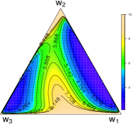
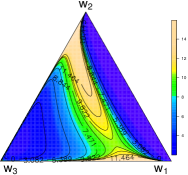
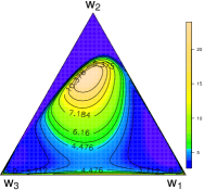
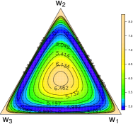
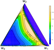
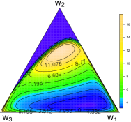
Figure 7: Trivariate extremal skew-$t$ angular densities with $\nu=3$ degrees of freedom. Correlation coefficients are $\omega=(0.6,0.8,0.7)^{\top}$ for the top row and $\omega=(0.7,0.7,0.7)^{\top}$ for the bottom. From left to right the skewness parameters are $\alpha=(0,0,0)^{\top}$, $\alpha=(-3,-3,7)^{\top}$ and $\alpha=(7,-10,3)^{\top}$. In all cases $\tau=0$ for simplicity.

Figure 7 illustrates some examples of the flexibility of the trivariate extremal-skew-$t$ dependence structure. Here we write the correlation coefficients as $\omega=(\omega_{1,2},\omega_{1,3},\omega_{2,3})^{\top}$ and the slant parameters as $\alpha=(\alpha_{1,2},\alpha_{1,3},\alpha_{2,3})^{\top}$, and assume that $\nu=3$ and $\tau=0$ for simplicity.

The plots in the left column have $\alpha=(0,0,0)^{\top}$ and so correspond to the extremal-$t$ angular measure. The density in the top-left panel, obtained with $\omega=(0.6,0.8,0.7)^{\top}$, has mass concentrations mainly on the edge that links the first and the third variable, since they are the most dependent ($w_{1,3}=0.8$). Some mass is also placed on the corners of the second variable, indicating that this is less dependent on the others ($w_{1,2}=0.6$ and $w_{2,3}=0.7$), and on the middle of the simplex, because a low degree of freedom ($\nu=3$) pushes mass towards the centre of the simplex. The top-middle and top-right panels are extremal skew-$t$ angular densities obtained with $\alpha=(-3,-3,7)^{\top}$ and $\alpha=(7,-10,3)^{\top}$ respectively. Here the impact of the slant parameters is to increase the levels of dependence – indeed the mass is clearly pushed towards the centre of the simplex. In the middle panel dependence between the second and third variables has increased, while in the right panel all variables are strongly dependent with a greater dependence of the second variable on the others.

The bottom row in Figure 7 illustrates the spectral densities with correlation coefficients $\omega=(0.7,0.7,0.7)^{\top}$. The bottom-left panel is the standard extremal-$t$ dependence (with $\alpha=(0,0,0)^{\top}$), which has a symmetric density with mass concentrated mainly in the centre of the simplex and on the vertices. The bottom-middle and bottom-right panels show extremal skew-$t$ densities, obtained with $\alpha=(-3,-3,7)^{\top}$ and $\alpha=(7,-10,3)^{\top}$ respectively. In this case the impact of the slant parameters is to decrease the dependence – here the mass is pushed towards the edges of the simplex. In the middle panel the first and second variables have become less dependent from the third variable, more so than between each other. In the right panel the first and third variables are less dependent on the second. These examples illustrate the great flexibility of the extremal skew-$t$ model in capturing a wide range of extremal dependence behaviour above and beyond that of the standard extremal $t$ model.

B.2 Display of the partitions of the three-dimensional simplex

Figure 8 displays the partitions of the three-dimensional simplex into three vertices (grey shading), edges (line shading) and the interior (no shading). Observations where angular components fall into such areas are considered to belong to the corresponding subset of the simplex (vertex, edge or interior).

$\begin{array}[]{cc}\includegraphics[width=216.81pt]{triangle_czone_v3-eps-converted-to.pdf}\end{array}$

Figure 8: Partitions of the three-dimensional simplex

For example, when $w_{3}>1-c$ (on the left of the green dashed line indicating the $1-c$ level for $w_{3}$), then $w=(w_{1},w_{2},w_{3})$ is in the corner associated with the third component, which corresponds to the grey shaded triangle on the bottom left of the simplex. Similarly, if both $w_{1}$ and $w_{2}$ are less than $1-c$ (i.e. to the left of the blue dashed line indicating the $1-c$ level of $w_{1}$ and below the red dashed line indicating the $1-c$ level of $w_{2}$), such that $w_{1}>1-2w_{2}$ and $w_{2}>1-2w_{1}$ (i.e. to the right of the black dashed line bisecting the corner of the second component and above the black dashed line bisecting the corner of the first component) and if $w_{3}<c$ (to the right of the green dashed line indicating the $1-c$ level of $w_{3}$) then $w=(w_{1},w_{2},w_{3})$ is on the edge between the first and second component. This is indicated by the line-shaded area on the right hand side of the simplex. Finally if $w_{1},w_{2},w_{3}>c$ (i.e. to the right of the blue dashed line, above the red dashed line and to the left of the green dashed line, respectively indicating the $c$ levels of $w_{1},w_{2}$ and $w_{3}$) then $w=(w_{1},w_{2},w_{3})$ is in the interior of the simplex, represented by the white triangle in the centre of the simplex.

B.3 Computation of $d$-dimensional extremal-skew-$t$ density for $d=2,3,4$.

For clarity of exposition we focus on the finite dimensional distribution of the extremal-$t$ process, denoted by $G$. We initially assume that $\alpha=0$ and $\tau=0$ in (15) of the main paper (focusing on (16)), and relax this assumption later. For brevity the exponent function is written as

$$V(x_{j},j\in I)=\sum_{j\in I}x_{j}^{-1}T_{j},\quad T_{j}=\Psi_{d-1}\left(u_{j};\bar{\Omega}^{\circ}_{j},\nu+1\right)$$

where $I=\{1,\ldots,d\}$, $u_{j}=\left[\sqrt{\frac{\nu+1}{1-\omega_{i,j}^{2}}}\left\{\left(\frac{x_{i}}{x_{j}}\right)^{1/\nu}-\omega_{i,j}\right\},i\in I_{j}\right]^{\top}$ and where $I_{j}=I\backslash\{j\}$. By successive differentiations the $2$-dimensional density ($d=2$) is

$$f(x)=(-V_{12}+V_{1}V_{2})G(x),\quad x\in{\mathbb{R}}_{+}^{2},$$

the $3$-dimensional density ($d=3$) is

$$f(x)=(-V_{123}+V_{1}V_{23}+V_{2}V_{13}+V_{3}V_{12}-V_{1}V_{2}V_{3})G(x),\quad x\in{\mathbb{R}}_{+}^{3}$$

and the $4$-dimensional density ($d=4$) is

$$f(x) =(-V_{1234}+V_{1}V_{234}+V_{2}V_{134}+V_{3}V_{124}+V_{12}V_{34}+V_{13}V_{24}+V_{14}V_{23}$$

$$\quad-V_{1}V_{2}V_{34}-V_{1}V_{3}V_{24}-V_{1}V_{4}V_{23}-V_{2}V_{3}V_{14}-V_{2}V_{4}V_{13}-V_{3}V_{4}V_{12}$$

$$\quad+V_{1}V_{2}V_{3}V_{4})G(x),\quad x\in{\mathbb{R}}_{+}^{4}$$

where $V_{i_{1},\ldots,i_{m}}:=\frac{\text{d}^{m}V(x_{j},j\in I)}{\text{d}x_{i_{1}}\cdots\text{d}x_{i_{m}}}$ for $i_{k}\in I$. The derivatives of the exponent function are given by

$$V_{i_{1},\ldots,i_{m}}=\sum_{k=1}^{d}x_{i_{k}}^{-1}\frac{\text{d}^{m}T_{i_{k}}}{\text{d}x_{i_{1}}\cdots\text{d}x_{i_{m}}}-\sum_{\ell=1}^{m}x_{i_{\ell}}^{-2}\frac{\text{d}^{m-1}T_{i_{\ell}}}{\text{d}x_{i_{1}}\cdots\text{d}x_{i_{\ell-1}}\text{d}x_{i_{\ell+1}}\cdots\text{d}x_{i_{m}}}.$$ (29)

In particular, when $m=d$ it follows that $\{i_{1},\ldots,i_{d}\}=\{1,\ldots,d\}$ and that

$$V_{1\cdots d}=-(\nu x_{1})^{-(d+1)}\psi_{d-1}\left(u_{1};\bar{\Omega}^{\circ}_{1},\nu+1\right)\prod_{i=2}^{d}\sqrt{\frac{\nu+1}{1-\omega_{i,1}^{2}}}\left(\frac{x_{i}}{x_{1}}\right)^{\frac{1}{\nu}-1}.$$

When $d=2$ or $3$, the derivatives of $T_{j}$, for $j\in I$ are given by

$$\frac{\text{d}T_{j}}{\text{d}x_{i_{1}}} =\sum_{p=1}^{d-1}\frac{\text{d}}{\text{d}u_{p,j}}\Psi_{d-1}\left(u_{j};\bar{\Omega}^{\circ}_{j},\nu+1\right)\frac{\text{d}u_{p,j}}{\text{d}x_{i_{1}}},$$ (30)

$$\frac{\text{d}^{2}T_{j}}{\text{d}x_{i_{1}}\text{d}x_{i_{2}}} =\sum_{p=1}^{d-1}\left(\frac{\text{d}}{\text{d}u_{p,j}}\Psi_{d-1}\left(u_{j};\bar{\Omega}^{\circ}_{j},\nu+1\right)\frac{\text{d}^{2}u_{p,j}}{\text{d}x_{i_{1}}\text{d}x_{i_{2}}}+\frac{\text{d}^{2}}{\text{d}u_{p,j}^{2}}\Psi_{d-1}\left(u_{j};\bar{\Omega}^{\circ}_{j},\nu+1\right)\frac{\text{d}u_{p,j}}{\text{d}x_{i_{1}}}\frac{\text{d}u_{p,j}}{\text{d}x_{i_{2}}}\right)$$

$$+\sum_{p=1}^{d-2}\sum_{q=p+1}^{d-1}\frac{\text{d}^{2}}{\text{d}u_{p,j}\text{d}u_{q,j}}\Psi_{d-1}\left(u_{j};\bar{\Omega}^{\circ}_{j},\nu+1\right)\left[\frac{\text{d}u_{p,j}}{\text{d}x_{i_{1}}}\frac{\text{d}u_{q,j}}{\text{d}x_{i_{2}}}+\frac{\text{d}u_{p,j}}{\text{d}x_{i_{2}}}\frac{\text{d}u_{q,j}}{\text{d}x_{i_{1}}}\right],$$ (31)

where $u_{p,j}$ is the $p$-th element of $u_{j}$, and when $d=3$

$$\frac{\text{d}^{3}T_{j}}{\text{d}x_{i_{1}}\text{d}x_{i_{2}}\text{d}x_{i_{3}}} =\sum_{p=1}^{2}\sum_{q=2}^{3}\left(\frac{\text{d}^{2}}{\text{d}u_{p,j}\text{d}u_{q,j}}\Psi_{d-1}\left(u_{j};\bar{\Omega}^{\circ}_{j},\nu+1\right)\sum_{\begin{subarray}{c}r,s,t\in I\\ r\neq s\neq t\end{subarray}}\frac{\text{d}u_{p,j}}{\text{d}x_{i_{r}}}\frac{\text{d}^{2}u_{q,j}}{\text{d}x_{i_{s}}\text{d}x_{i_{t}}}+\frac{\text{d}u_{q,j}}{\text{d}x_{i_{r}}}\frac{\text{d}^{2}u_{p,j}}{\text{d}x_{i_{s}}\text{d}x_{i_{t}}}\right)$$

$$+\sum_{p=1}^{3}\sum_{\begin{subarray}{c}q=1\\ q\neq p\end{subarray}}^{3}\frac{\text{d}^{3}}{\text{d}u_{p,j}^{2}\text{d}u_{q,j}}\Psi_{d-1}\left(u_{j};\bar{\Omega}^{\circ}_{j},\nu+1\right)\sum_{\begin{subarray}{c}r,s,t\in I\\ r\neq s\neq t\end{subarray}}\frac{\text{d}u_{p,j}}{\text{d}x_{i_{r}}}\frac{\text{d}u_{p,j}}{\text{d}x_{i_{s}}}\frac{\text{d}u_{q,j}}{\text{d}x_{i_{t}}}$$

$$+\frac{\text{d}^{3}}{\text{d}u_{1,j}\text{d}u_{2,j}\text{d}u_{3,j}}\Psi_{d-1}\left(u_{j};\bar{\Omega}^{\circ}_{j},\nu+1\right)\sum_{\begin{subarray}{c}r,s,t\in I\\ r\neq s\neq t\end{subarray}}\frac{\text{d}u_{1,j}}{\text{d}x_{i_{r}}}\frac{\text{d}u_{2,j}}{\text{d}x_{i_{s}}}\frac{\text{d}u_{3,j}}{\text{d}x_{i_{t}}}.$$ (32)

We provide the derivatives of the $d$-dimensional $t$ cdf below. When $d=1$ and for all $x\in{\mathbb{R}}_{+}$

$$\frac{\text{d}}{\text{d}x}\Psi(x;\nu) =\psi(x;\nu),\quad\frac{\text{d}^{2}}{\text{d}x^{2}}\Psi(x;\nu)=-\frac{(\nu+1)x}{\nu+x^{2}}\psi(x;\nu),$$

$$\frac{\text{d}^{3}}{\text{d}x^{3}}\Psi(x;\nu) =\frac{(\nu+1)(x^{2}-\nu+(\nu+1)x^{2})}{(\nu+x^{2})^{2}}\psi(x;\nu).$$

When $d=2$ and for all $x\in{\mathbb{R}}_{+}^{2}$,

$$\frac{\text{d}}{\text{d}x_{1}}\Psi_{2}(x;\bar{\Omega},\nu) =\psi(x_{1};\nu)\Psi\left(v_{2\cdot 1};\nu+1\right),$$

$$\frac{\text{d}^{2}}{\text{d}x_{1}^{2}}\Psi_{2}(x;\bar{\Omega},\nu) =-\psi(x_{1};\nu)\left\{\frac{(\nu+1)x_{1}}{\nu+x_{1}^{2}}\Psi\left(v_{2\cdot 1};\nu+1\right)+\sqrt{\frac{\nu+1}{1-\omega^{2}}}\left(\frac{\omega\nu+x_{2}x_{1}}{(\nu+x_{1}^{2})^{3/2}}\right)\psi\left(v_{2\cdot 1};\nu+1\right)\right\},$$

$$\frac{\text{d}^{2}}{\text{d}x_{1}\text{d}x_{2}}\Psi_{2}(x;\bar{\Omega},\nu) =\psi_{2}(x;\bar{\Omega},\nu),$$

where $v_{i\cdot j}=\sqrt{\frac{\nu+1}{\nu+x_{j}^{2}}}\frac{x_{i}-\omega_{i,j}x_{1}}{\sqrt{1-\omega_{i,j}^{2}}},\quad j\in I,j\in I_{j},$

$$\frac{\text{d}^{3}}{\text{d}x_{1}^{3}}\Psi_{2}(x;\bar{\Omega},\nu) =\Psi\left(v_{2\cdot 1};\nu+1\right)\psi(x_{1};\nu)\left\{\frac{(\nu+1)^{2}x_{1}^{2}-(\nu+1)(\nu-x_{1}^{2})}{(\nu+x_{1}^{2})^{2}}\right\}$$

$$+\psi\left(v_{2\cdot 1};\nu+1\right)\psi(x_{1};\nu)\sqrt{\frac{\nu+1}{1-\omega^{2}}}\frac{1}{(\nu+x_{1}^{2})^{5/2}}$$

$$\times\left\{x_{1}(\omega\nu+x_{2}x_{1})(2\nu-1)-x_{2}(\nu+x_{1}^{2})\right.$$

$$-\left.\frac{\big{(}\omega(\nu+x_{1}^{2})+(x_{2}-\omega x_{1})x_{1}\big{)}(\nu+2)(x_{2}-\omega x_{1})(\omega\nu+x_{2}x_{1})}{(\nu+x_{1}^{2})(1-\omega^{2})+(x_{2}-\omega x_{1})^{2}}\right\},$$

$$\frac{\text{d}^{3}}{\text{d}x_{1}^{2}\text{d}x_{2}}\Psi_{2}(x;\bar{\Omega},\nu) =-\frac{(\nu+2)(x_{1}-\omega x_{2})}{2\pi\nu(1-\omega^{2})^{3/2}}\bigg{(}1+\frac{x_{1}^{2}-2\omega x_{1}x_{2}+x_{2}^{2}}{\nu(1-\omega^{2})}\bigg{)}^{-(\frac{\nu}{2}+1)}.$$

When $d=3$ and for all $x\in{\mathbb{R}}_{+}^{3}$,

$$\frac{\text{d}}{\text{d}x_{1}}\Psi_{3}(x;\bar{\Omega},\nu) =\psi(x;\nu)\Psi_{2}\left\{(v_{2\cdot 1},v_{3\cdot 1})^{\top};\bar{\Omega}^{\circ}_{1},\nu+1\right\},$$

$$\frac{\text{d}^{2}}{\text{d}x_{1}^{2}} \Psi_{3}(x;\bar{\Omega},\nu)=\frac{-\psi(x_{1};\nu)}{\nu+x_{1}^{2}}\left[(\nu+1)x_{1}\times\Psi_{2}\left\{(v_{2\cdot 1},v_{3\cdot 1})^{\top};\bar{\Omega}^{\circ}_{1},\nu+1\right\}\right.$$

$$+\psi\left(v_{2\cdot 1};\nu+1\right)\sqrt{\frac{\nu+1}{1-\omega_{12}^{2}}}\frac{x_{2}x_{1}+\omega_{12}\nu}{\sqrt{\nu+x_{1}^{2}}}$$

$$\times\Psi\left(\frac{\sqrt{\nu+2}\left\{(x_{3}-\omega_{13}x_{1})(1-\omega_{12}^{2})-(\omega_{23}-\omega_{12}\omega_{13})(x_{2}-\omega_{12}x_{1})\right\}}{\sqrt{\left\{(1-\omega_{12}^{2})(\nu+x_{1}^{2})+(x_{2}-\omega_{12}x_{1})^{2}\right\}\left\{(1-\omega_{12}^{2})(1-\omega_{13}^{2})-(\omega_{23}-\omega_{12}\omega_{13})^{2}\right\}}};\nu+2\right)$$

$$+\psi\left(v_{3\cdot 1};\nu+1\right)\sqrt{\frac{\nu+1}{1-\omega_{13}^{2}}}\frac{x_{3}x_{1}+\omega_{13}\nu}{\sqrt{\nu+x_{1}^{2}}}$$

$$\times\left.\Psi\left(\frac{\sqrt{\nu+2}\left\{(x_{2}-\omega_{12}x_{1})(1-\omega_{13}^{2})-(\omega_{23}-\omega_{12}\omega_{13})(x_{3}-\omega_{13}x_{1})\right\}}{\sqrt{\left\{(1-\omega_{13}^{2})(\nu+x_{1}^{2})+(x_{3}-\omega_{13}x_{1})^{2}\right\}\left\{(1-\omega_{12}^{2})(1-\omega_{13}^{2})-(\omega_{23}-\omega_{12}\omega_{13})^{2}\right\}}};\nu+2\right)\right]$$

$$\frac{\text{d}^{2}}{\text{d}x_{1}\text{d}x_{2}} \Psi_{3}(x;\bar{\Omega},\nu)=\psi(x_{2};\nu)\psi\left(v_{1\cdot 2};\nu+1\right)\sqrt{\frac{\nu+1}{(1-\omega_{12}^{2})(\nu+x_{2}^{2})}}$$

$$\times\Psi\left(\frac{\sqrt{\nu+2}\left\{(x_{3}-\omega_{23}x_{2})(1-\omega_{12}^{2})-(\omega_{13}-\omega_{12}\omega_{23})(x_{1}-\omega_{12}x_{2})\right\}}{\sqrt{\left\{(1-\omega_{12}^{2})(\nu+x_{1}^{2})+(x_{1}-\omega_{12}x_{2})^{2}\right\}\left\{(1-\omega_{12}^{2})(1-\omega_{23}^{2})-(\omega_{13}-\omega_{12}\omega_{23})^{2}\right\}}};\nu+2\right)$$

$$\frac{\text{d}^{3}}{\text{d}x_{1}^{2}\text{d}x_{2}} \Psi_{3}(x;\bar{\Omega},\nu)=-\psi(x_{3};\nu)\psi\left(v_{1\cdot 3};\nu+1\right)\sqrt{\frac{\nu+1}{(1-\omega_{13}^{2})(\nu+x_{3}^{2})}}\left[\frac{(\nu+2)(x_{1}-\omega_{12}x_{2})}{(1-\omega_{12}^{2})(\nu+x_{2}^{2})+(x_{1}-\omega_{12}x_{2})^{2}}\right.$$

$$\times\Psi\left(\frac{\sqrt{\nu+2}\left\{(x_{3}-\omega_{23}x_{2})(1-\omega_{12}^{2})-(\omega_{13}-\omega_{12}\omega_{23})(x_{1}-\omega_{12}x_{2})\right\}}{\sqrt{\left\{(1-\omega_{12}^{2})(\nu+x_{1}^{2})+(x-\omega_{12}x_{2})^{2}\right\}\left\{(1-\omega_{12}^{2})(1-\omega_{23}^{2})-(\omega_{13}-\omega_{12}\omega_{23})^{2}\right\}}};\nu+2\right)$$

$$+\frac{\sqrt{\nu+2}(1-\omega_{12}^{2})}{\sqrt{(1-\omega_{12}^{2})(1-\omega_{23}^{2})-(\omega_{13}-\omega_{12}\omega_{23})^{2}}}\frac{(\omega_{13}-\omega_{12}\omega_{23})-(x_{1}-\omega_{12}x_{2})(x_{3}-\omega_{23}x_{2})}{\left\{(1-\omega_{12}^{2})(\nu+x_{2}^{2})+(x_{1}-\omega_{12}x_{2})^{2}\right\}^{3/2}}$$

$$\times\left.\psi\left(\frac{\sqrt{\nu+2}\left\{(x_{3}-\omega_{23}x_{2})(1-\omega_{12}^{2})-(\omega_{13}-\omega_{12}\omega_{23})(x_{1}-\omega_{12}x_{2})\right\}}{\sqrt{\left\{(1-\omega_{12}^{2})(\nu+x_{1}^{2})+(x_{1}-\omega_{12}x_{2})^{2}\right\}\left\{(1-\omega_{12}^{2})(1-\omega_{23}^{2})-(\omega_{13}-\omega_{12}\omega_{23})^{2}\right\}}};\nu+2\right)\right]$$

$$\frac{\text{d}^{3}}{\text{d}x_{1}^{3}} \Psi_{3}(x;\bar{\Omega},\nu)=-\frac{\psi(x_{1};\nu)}{(\nu+x_{1}^{2})}\left[\left(\frac{\nu+3}{\nu+x_{1}^{2}}\right)(1-x_{1}^{2})(\nu+1)\Psi_{2}\left\{(v_{2\cdot 1},v_{3\cdot 1})^{\top};\bar{\Omega}^{\circ}_{1},\nu+1\right\}\right.$$

$$+\Psi\left(\frac{\sqrt{\nu+2}\left[(x_{3}-\omega_{13}x_{1})(1-\omega_{12}^{2})-(\omega_{23}-\omega_{12}\omega_{13})(x_{2}-\omega_{12}x_{1})\right]}{\sqrt{\left[(1-\omega_{12}^{2})(\nu+x_{1}^{2})+(x_{2}-\omega_{12}x_{1})^{2}\right]\left[(1-\omega_{12}^{2})(1-\omega_{13}^{2})-(\omega_{23}-\omega_{12}\omega_{13})^{2}\right]}};\nu+2\right)$$

$$\times\psi\left(v_{2\cdot 1};\nu+1\right)\sqrt{\frac{\nu+1}{1-\omega_{12}^{2}}}\frac{2(x_{2}x_{1}+\omega_{12}\nu)(\nu+2)x_{1}-\nu(x_{2}-\omega_{12}x_{1})}{(\nu+x_{1}^{2})^{3/2}}$$

$$\times\frac{(\nu+2)(x_{2}-\omega_{12}x_{1})\sqrt{\nu+1}(x_{2}x_{1}+\omega_{12}\nu)^{2}}{\sqrt{1-\omega_{12}^{2}}(\nu+x_{1}^{2})^{3/2}\left((1-\omega_{12}^{2})(\nu+x_{1}^{2})+(x_{2}-\omega_{12}x_{1})^{2}\right)}$$

$$+\Psi\left(\frac{\sqrt{\nu+2}\left[(x_{2}-\omega_{12}x_{1})(1-\omega_{13}^{2})-(\omega_{23}-\omega_{12}\omega_{13})(x_{3}-\omega_{13}x_{1})\right]}{\sqrt{\left[(1-\omega_{13}^{2})(\nu+x_{1}^{2})+(x_{3}-\omega_{13}x_{1})^{2}\right]\left[(1-\omega_{12}^{2})(1-\omega_{13}^{2})-(\omega_{23}-\omega_{12}\omega_{13})^{2}\right]}};\nu+2\right)$$

$$\times\psi\left(v_{3\cdot 1};\nu+1\right)\sqrt{\frac{\nu+1}{1-\omega_{13}^{2}}}\frac{2(x_{3}x_{1}+\omega_{13}\nu)(\nu+2)x_{1}-\nu(x_{3}-\omega_{13}x_{1})}{(\nu+x_{1}^{2})^{3/2}}$$

$$\times\frac{(\nu+2)(x_{3}-\omega_{13}x_{1})\sqrt{\nu+1}(x_{3}x_{1}+\omega_{13}\nu)^{2}}{\sqrt{1-\omega_{13}^{2}}(\nu+x_{1}^{2})^{3/2}\left((1-\omega_{13}^{2})(\nu+x_{1}^{2})+(x_{3}-\omega_{13}x_{1})^{2}\right)}~$$

$$+\psi\left(\frac{\sqrt{\nu+2}\left[(x_{3}-\omega_{13}x_{1})(1-\omega_{12}^{2})-(\omega_{23}-\omega_{12}\omega_{13})(x_{2}-\omega_{12}x_{1})\right]}{\sqrt{\left[(1-\omega_{12}^{2})(\nu+x_{1}^{2})+(x_{2}-\omega_{12}x_{1})^{2}\right]\left[(1-\omega_{12}^{2})(1-\omega_{13}^{2})-(\omega_{23}-\omega_{12}\omega_{13})^{2}\right]}};\nu+2\right)$$

$$\times\psi\left(v_{2\cdot 1};\nu+1\right)\sqrt{\frac{(1-\omega_{12}^{2})(\nu+2)}{(1-\omega_{12}^{2})(1-\omega_{13}^{2})-(\omega_{23}-\omega_{12}\omega_{13})^{2}}}$$

$$\times\frac{\sqrt{\nu+1}(x_{2}x_{1}+\omega_{12}\nu)}{\sqrt{\nu+x_{1}^{2}}((1-\omega_{12}^{2})(\nu+x_{1}^{2})+(x_{2}-\omega_{12}x_{1})^{2})^{3/2}}\bigg{[}((1-\omega_{12}^{2})(\nu+x_{1}^{2})+(x_{2}-\omega_{12}x_{1})^{2})$$

$$\times\left(\omega_{12}\frac{\omega_{23}-\omega_{12}\omega_{13}}{1-\omega_{12}^{2}}-\omega_{13}\right)-\left((x_{3}-\omega_{13}x_{1})-\frac{\omega_{23}-\omega_{12}\omega_{13}}{1-\omega_{12}^{2}}(x_{2}-\omega_{12}x_{1})\right)(x_{1}-\omega_{12}x_{2})\bigg{]}$$

$$+\psi\left(\frac{\sqrt{\nu+2}\left[(x_{2}-\omega_{12}x_{1})(1-\omega_{13}^{2})-(\omega_{23}-\omega_{12}\omega_{13})(x_{3}-\omega_{13}x_{1})\right]}{\sqrt{\left[(1-\omega_{13}^{2})(\nu+x_{1}^{2})+(x_{3}-\omega_{13}x_{1})^{2}\right]\left[(1-\omega_{12}^{2})(1-\omega_{13}^{2})-(\omega_{23}-\omega_{12}\omega_{13})^{2}\right]}};\nu+2\right)$$

$$\times\psi\left(v_{3\cdot 1};\nu+1\right)\sqrt{\frac{(1-\omega_{13}^{2})(\nu+2)}{(1-\omega_{12}^{2})(1-\omega_{13}^{2})-(\omega_{23}-\omega_{12}\omega_{13})^{2}}}$$

$$\times\frac{\sqrt{\nu+1}(x_{3}x_{1}+\omega_{13}\nu)}{\sqrt{\nu+x_{1}^{2}}((1-\omega_{13}^{2})(\nu+x_{1}^{2})+(x_{3}-\omega_{13}x_{1})^{2})^{3/2}}\bigg{[}((1-\omega_{13}^{2})(\nu+x_{1}^{2})+(x_{3}-\omega_{13}x_{1})^{2})$$

$$\times\left(\omega_{13}\frac{\omega_{23}-\omega_{12}\omega_{13}}{1-\omega_{13}^{2}}-\omega_{12}\right)-\left((x_{2}-\omega_{12}x_{1})-\frac{\omega_{23}-\omega_{12}\omega_{13}}{1-\omega_{13}^{2}}(x_{3}-\omega_{13}x)\right)(x_{1}-\omega_{13}x_{3})\bigg{]}.$$

Combining the derivatives of the $t$ cdf with equations (29)–(B.3) provides the full $d$-dimensional densities of the extremal-$t$ process. Returning to the extremal skew-$t$ case (i.e. when $\alpha\neq 0$ and $\tau\neq 0$), it is sufficient to consider the following changes. Firstly, rewrite

$$T_{j}=\frac{\Psi_{d}\left\{\left(\begin{array}[]{c}u_{j}\\ \bar{\tau}_{j}\end{array}\right);\left(\begin{array}[]{cc}\bar{\Omega}^{\circ}_{j}&-\delta_{j}\\ -\delta_{j}^{\top}&1\end{array}\right),\nu+1\right\}}{\Psi_{1}\left(\bar{\tau}_{j};\nu+1\right)},\quad j\in I,$$

where $u_{j}=\left[\sqrt{\frac{\nu+1}{1-\omega_{i,j}^{2}}}\left\{\left(\frac{x_{i}^{\circ}}{x_{j}^{\circ}}\right)^{1/\nu}-\omega_{i,j}\right\},i\in I_{j}\right]^{\top},$ following Definition 1 of the main paper. It can then be shown that

$$V_{1\cdots d}=-(\nu x_{1})^{-(d+1)}\psi_{d-1}(u_{1};\bar{\Omega}^{\circ}_{1},\alpha_{1}^{\circ},\tau_{1}^{\circ},\kappa_{1}^{\circ},\nu+1)\prod_{i=2}^{d}\sqrt{\frac{\nu+1}{1-\omega_{i,1}^{2}}}\left(\frac{x^{\circ}_{i}}{x^{\circ}_{1}}\right)^{\frac{1}{\nu}-1}\frac{m_{i}^{+}}{m_{1}^{+}}$$

following Theorem 1 of the main paper. Note that equations (29)–(B.3) are still valid in this case, through the redefinition of $d\leftarrow d+1$ and $u_{j}\leftarrow(u_{j},\bar{\tau}_{j})^{\top}$. This in combination with the above derivatives of the $t$ cdfs leads to the $d$-dimensional densities of the extremal-skew-$t$ process.

$\nu=1$
$n=20$
$\lambda\backslash\xi$	$0.5$	$1$	$1.5$	$1.9$	$2$
$14$	$89/94/89$	$84/97/93$	$83/69/79$	$81/82/84$	$78/64/72$
$28$	$76/100/98$	$59/100/69$	$73/86/73$	$74/66/75$	$34/75/26$
$42$	$81/100/100$	$51/96/89$	$51/80/88$	$43/63/79$	$33/51/72$
$n=50$
$\lambda\backslash\xi$	$0.5$	$1$	$1.5$	$1.9$	$2$
$14$	$85/81/84$	$87/78/86$	$76/67/78$	$66/56/72$	$52/47/62$
$28$	$64/100/81$	$81/79/82$	$73/72/78$	$72/66/74$	$34/68/24$
$42$	$71/100/97$	$33/61/59$	$17/42/40$	$17/34/37$	$2/18/7$
$n=70$
$\lambda\backslash\xi$	$0.5$	$1$	$1.5$	$1.9$	$2$
$14$	$80/87/83$	$81/76/80$	$74/65/77$	$62/57/70$	$47/42/60$
$28$	$51/100/68$	$82/82/84$	$72/72/77$	$71/66/73$	$54/53/62$
$42$	$56/93/89$	$28/52/48$	$13/40/14$	$12/28/27$	$8/23/26$
$\nu=3$
$n=20$
$\lambda\backslash\xi$	$0.5$	$1$	$1.5$	$1.9$	$2$
$14$	$93/100/96$	$93/96/91$	$88/84/83$	$84/83/84$	$78/77/82$
$28$	$86/100/100$	$72/97/75$	$90/91/89$	$87/85/86$	$39/78/50$
$42$	$78/100/100$	$72/97/100$	$58/71/74$	$51/68/95$	$44/58/84$
$n=50$
$\lambda\backslash\xi$	$0.5$	$1$	$1.5$	$1.9$	$2$
$14$	$91/85/89$	$92/89/92$	$86/81/88$	$82/78/86$	$64/64/74$
$28$	$70/100/81$	$74/87/63$	$83/81/84$	$80/74/82$	$77/75/81$
$42$	$69/100/100$	$47/70/75$	$36/53/64$	$30/40/61$	$38/32/33$
$n=70$
$\lambda\backslash\xi$	$0.5$	$1$	$1.5$	$1.9$	$2$
$14$	$93/93/94$	$89/88/87$	$81/77/85$	$81/74/84$	$58/58/71$
$28$	$94/94/94$	$85/87/89$	$81/77/86$	$79/75/82$	$81/77/84$
$42$	$65/94/95$	$44/57/62$	$29/45/49$	$25/35/50$	$20/28/38$

Table 3: Efficiency of maximum triplewise likelihood estimators relative to maximum pairwise likelihood estimators for the Extremal-$t$ process, based on $300$ replicate simulations. Simulated datasets of size $n=20,50,70$ are generated at $20$ random sites in $\mathbb{S}=\left[0,100\right]^{2}$, given power exponential dependence function parameters $\vartheta=(\lambda,\xi)$. Relative efficiencies are $RE_{\xi}$/$RE_{\lambda}$/$RE_{(\lambda,\xi)}$ ($\times 100$) where $RE_{\xi}=\widehat{\text{var}}(\hat{\xi}_{3})/\widehat{\text{var}}(\hat{\xi}_{2})$, $RE_{\lambda}=\widehat{\text{var}}(\hat{\lambda}_{3})/\widehat{\text{var}}(\hat{\lambda}_{2})$ and $RE_{(\lambda,\xi)}=\widehat{\text{cov}}(\hat{\lambda}_{3},\hat{\xi}_{3})/\widehat{\text{cov}}(\hat{\lambda}_{2},\hat{\xi}_{2})$, where $(\hat{\lambda}_{m},\hat{\xi}_{m})$ are the $m$-wise maximum composite likelihood estimates ($m=2,3$), and $\widehat{\text{var}}$ and $\widehat{\text{cov}}$ denote sample variance and covariance over replicates.

B.4 Composite likelihood simulation study

We compare the efficiency of the maximum triplewise composite likelihood estimator with that based on the pairwise composite likelihood, discussed in Section 4 of the main paper, when data are drawn from an extremal-$t$ process. We generate 300 replicate samples of size $n=20,50$ and $70$ from the extremal-$t$ process with correlation function (10) in Section 2.2 of the main paper, with varying parameters, over $20$ random spatial points on $\mathbb{S}=[0,100]^{2}$. Table 3 presents the resulting relative efficiencies $RE_{\xi}$/$RE_{\lambda}$/$RE_{(\lambda,\xi)}$ ($\times 100$), where $RE_{\xi}=\widehat{\text{var}}(\hat{\xi}_{3})/\widehat{\text{var}}(\hat{\xi}_{2})$, $RE_{\lambda}=\widehat{\text{var}}(\hat{\lambda}_{3})/\widehat{\text{var}}(\hat{\lambda}_{2})$ and $RE_{(\lambda,\xi)}=\widehat{\text{cov}}(\hat{\lambda}_{3},\hat{\xi}_{3})/\widehat{\text{cov}}(\hat{\lambda}_{2},\hat{\xi}_{2})$, where $(\hat{\lambda}_{m},\hat{\xi}_{m})$ are the $m$-wise maximum composite likelihood estimates ($m=2,3$), and $\widehat{\text{var}}$ and $\widehat{\text{cov}}$ denote sample variance and covariance over replicates. Perhaps unsurprisingly, the triplewise estimates are at worst just as efficient as the pairwise estimates ($RE\leq 100$) but are frequently much more efficient. However this is balanced computationally as there is a corresponding increase in the number of components in the triplewise composite likelihood function. For each $\nu$, there is a general gain in efficiency when the smoothing parameter $\xi$ increases for each fixed scale parameter $\lambda$. There is a similar gain when increasing $\lambda$ for fixed $\xi$. These gains become progressively pronounced with increasing sample size $n$, and when there is stronger dependence present (i.e. smaller degrees of freedom $\nu$). However, we note that there are a number of instances where the efficiency gain goes against this general trend, which indicates that there are some subtleties involved.

B.5 Marginal analysis of wind speed data

The maximum daily observations of wind speed ($1564$ observations per station) are considered for each of the $4$ monitoring stations CLOU, CLAY, SALL and PAUL. The $t$ and skew-$t$ distributions are fitted to the data using the maximum likelihood approach and a chi-square test is performed in order to investigate wether the slant parameter of the skew-$t$ distribution is significantly different from zero. Additionally the Fisher-Pearson coefficient of skewness ($\gamma$) is calculated.

Station	Model	$\hat{\mu}$	$\hat{\sigma}$	$\hat{\alpha}$	$\hat{\nu}$	$p$-value	$\gamma$
CLOU	$t$	$11.84$	$2.75$	$-$	$5.78$	$-$	$-$
	skew-$t$	$8.51$	$20.24$	$2.79$	$11.21$	$0$	$1.17$
CLAY	$t$	$12.63$	$3.50$	$-$	$6.40$	$-$	$-$
	skew-$t$	$8.23$	$35.53$	$3.28$	$16.61$	$0$	$1.12$
SALL	$t$	$14.66$	$4.27$	$-$	$7.47$	$-$	$-$
	skew-$t$	$9.02$	$58.76$	$4.20$	$50.98$	$0$	$0.92$
PAUL	$t$	$15.76$	$4.25$	$-$	$9.31$	$-$	$-$
	skew-$t$	$11.43$	$38.55$	$1.78$	$17.81$	$0$	$0.79$

Table 4: Outcome of the marginal analysis of the four stations.

The marginal estimation results are collected in Table 4. The estimated parameters are location $\mu$, scale $\sigma$ and degrees of freedom $\nu$ for the $t$ distribution and in addition the slant $\alpha$ for the skew-$t$ distributions. The Table also displays the $p$-value of a chi-square test of $\alpha=0$ for each station. With a $p$-value of effectively zero, the marginal skewness of the data is established for each station.

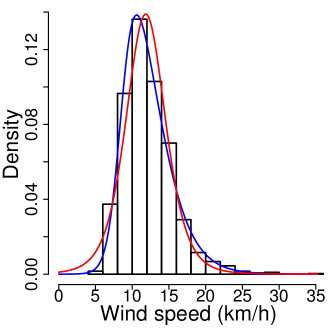
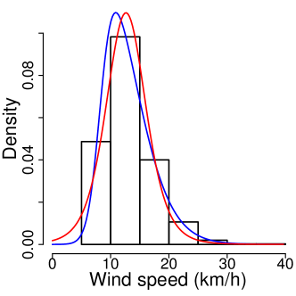
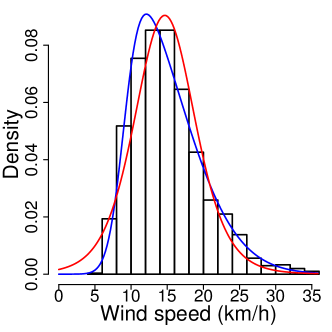
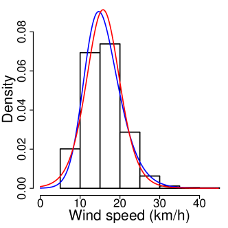
Figure 9: Histogram of daily windspeed data, fitted $t$ (red solid line) and skew-$t$ (blue solid line) densities for each of the four stations CLOU (top-left), CLAY (top-right), SALL (bottom-left) and PAUL (bottom-right).

The red and blue solid lines in Figure 9 respectively show the fitted $t$ and skew-$t$ densities compared to the histogram of the daily observations for each of the four monitoring stations. Each of the plots clearly shows that the datasets are right skewed and that the model with the ability to handle skewness provides a better fit.

References

• Arellano-Valle and Azzalini (2006) Arellano-Valle, R. B. and A. Azzalini (2006). On the unification of families of skew-normal distributions. Scand. J. Statist., 561–574.
• Arellano-Valle and Genton (2010) Arellano-Valle, R. B. and M. G. Genton (2010). Multivariate extended skew-$t$ distributions and related families. Metron 68(3), 201–234.
• Azzalini (1985) Azzalini, A. (1985). A class of distributions which includes the normal ones. Scand. J. Statist., 171–178.
• Azzalini (2005) Azzalini, A. (2005). The skew-normal distribution and related multivariate families. Scand. J. Statist. 32(2), 159–200. With discussion by Marc G. Genton and a rejoinder by the author.
• Azzalini (2013) Azzalini, A. (2013). The skew-normal and related families, Volume 3. Cambridge University Press.
• Beranger et al. (2015) Beranger, B., G. Marcon, and S. Padoan (2015). ExtremalDep: Extremal Dependence Modeling. R package version 0.1-2/r76.
• Bortot (2010) Bortot, P. (2010). Tail dependence in bivariate skew-normal and skew-$t$ distributions. Unpublished manuscript.
• Brown and Resnick (1977) Brown, B. M. and S. I. Resnick (1977). Extreme values of independent stochastic processes. J. Appl. Probab., 732–739.
• Chan and Wood (1997) Chan, G. and A. T. Wood (1997). Algorithm AS 312: An algorithm for simulating stationary Gaussian random fields. J. R. Stat. Soc. Ser. C. Appl. Stat. 46(1), 171–181.
• Chang and Genton (2007) Chang, S.-M. and M. G. Genton (2007). Extreme value distributions for the skew-symmetric family of distributions. Comm. Statist. Theory Methods 36(9), 1705–1717.
• Coles et al. (2003) Coles, S. G., L. R. Pericchi, and S. A. Sisson (2003). A fully probabilistic approach to extreme value modelling. Journal of Hydrology 273, 35–50.
• Coles and Tawn (1991) Coles, S. G. and J. A. Tawn (1991). Modelling extreme multivariate events. J. R. Stat. Soc. Ser. B. Stat. Methodol. 53(2), pp. 377–392.
• Coles and Tawn (1994) Coles, S. G. and J. A. Tawn (1994). Statistical methods for multivariate extremes: An application to structural design. J. R. Stat. Soc. Ser. C. Appl. Stat. 43(1), pp. 1–48.
• Davison and Gholamrezaee (2012) Davison, A. C. and M. M. Gholamrezaee (2012). Geostatistics of extremes. Proceedings of the Royal Society of London Series A: Mathematical and Physical Sciences 468, 581–608.
• Davison et al. (2012) Davison, A. C., S. A. Padoan, and M. Ribatet (2012). Statistical modeling of spatial extremes. Statist. Sci. 27, 161–186.
• de Haan (1984) de Haan, L. (1984). A spectral representation for max-stable processes. Ann. Appl. Probab. 12(4), 1194–1204.